Emulation of stochastic simulators using generalized lambda models

Abstract

Stochastic simulators are ubiquitous in many fields of applied sciences and engineering. In the context of uncertainty quantification and optimization, a large number of simulations is usually necessary, which becomes intractable for high-fidelity models. Thus surrogate models of stochastic simulators have been intensively investigated in the last decade. In this paper, we present a novel approach to surrogating the response distribution of a stochastic simulator which uses generalized lambda distributions, whose parameters are represented by polynomial chaos expansions of the model inputs. As opposed to most existing approaches, this new method does not require replicated runs of the simulator at each point of the experimental design. We propose a new fitting procedure which combines maximum conditional likelihood estimation with (modified) feasible generalized least-squares. We compare our method with state-of-the-art nonparametric kernel estimation on four different applications stemming from mathematical finance and epidemiology. Its performance is illustrated in terms of the accuracy of both the mean/variance of the stochastic simulator and the response distribution. As the proposed approach can also be used with experimental designs containing replications, we carry out a comparison on two of the examples, showing that replications do not necessarily help to get a better overall accuracy and may even worsen the results (at a fixed total number of runs of the simulator).

1 Introduction

With increasing demands on the functionality and performance of modern engineering systems, design and maintenance of complex products and structures require advanced computational models, a.k.a. simulators. They help assess the reliability and optimize the behavior of the system already at the design phase. Classical simulators are usually deterministic because they implement solvers for the governing equation of the system. Thus, repeated model evaluations with the same input parameters consistently result in the same value of the output quantities of interest (QoIs). In contrast, stochastic simulators contain intrinsic randomness, which leads to the QoI being a random variable conditioned on the given set of input parameters. In other words, each model evaluation with the same input values generates a realization of the response random variable that follows an unknown distribution. Formally, a stochastic simulator ${\mathcal{M}}_{s}$ can be expressed as

$$\begin{split}{\mathcal{M}}_{s}:{\mathcal{D}}_{\bm{X}}\times\Omega&\rightarrow{\mathbb{R}}\\ (\bm{x},\omega)&\mapsto{\mathcal{M}}_{s}(\bm{x},\omega),\end{split}$$ (1)

where $\bm{x}$ is the input vector that belongs to the input space ${\mathcal{D}}_{\bm{X}}$, and $\Omega$ denotes the sample space of the probability space $\left\{\Omega,\mathcal{F},\mathbb{P}\right\}$ that represents the internal source of randomness.

Stochastic simulators are widely used in modern engineering, finance, and medical sciences. Typical examples include evaluating the performance of a wind turbine under stochastic loads [1], predicting the price of an option in financial markets [2], and the spread of a disease in epidemiology [3].

Due to the random nature of stochastic simulators, repeated model evaluations with the same input parameters, called hereinafter replications, are necessary to fully characterize the probability distribution of the corresponding QoI. In addition, uncertainty quantification and optimization problems typically require model evaluations for various sets of input parameters. Altogether, it is necessary to have a large number of model runs, which becomes intractable for costly models. To alleviate the computational burden, surrogate models, a.k.a. emulators, can be used to replace the original model. Such a model emulates the input-output relation of the simulator and is easy and cheap to evaluate.

Among several options for constructing surrogate models, this paper focuses on the so-called nonintrusive approaches. More precisely, the computational model is considered as a “black box” and is only required to be evaluated on a limited number of input values, called the experimental design (ED).

Three classes of methods can be found in the literature for emulating the entire response distribution of a stochastic code in a nonintrusive manner. The first one is the random field approach, which approximates the stochastic simulator by a random field. The definition in Eq. 1 implies that a stochastic simulator can be regarded as a random field indexed by its input variables. Controlling the intrinsic randomness allows one to get access to different trajectories of the simulator, which are deterministic functions of the input variables. In practice, this is achieved by fixing the random seed inside the simulator. Evaluations of the trajectories over the experimental design can then be extended to continuous trajectories, either by classical surrogate methods [4] or through Karhunen–Loève expansions [5]. Since this approach requires the effective access to the random seed, it is only applicable to data generated in a specific way.

Another class of methods is the replication-based approach, which relies on using replications at all points of the experimental design to represent the response distribution through a suitable parametrization. The estimated distribution parameters are then treated as (noisy) outputs of a deterministic simulator. Then, conventional surrogate modeling methods, such as Gaussian processes [6] and polynomial chaos expansions (PCEs) [7], can emulate these parameters as a function of the model input [8, 9]. Because this approach employs two separate steps, the surrogate quality depends on the accuracy of the distribution estimation from replicates in the first step [10]. Therefore, many replications are necessary, especially when nonparametric estimators are used for the local inference [8, 9].

A third class of methods, known as the statistical approach, does not require replications or controlling the random seed. If the response distribution belongs to the exponential family, generalized linear models [11] and generalized additive models [12] can be efficiently applied. When the QoI for a given set of input parameters follows an arbitrary distribution, nonparametric estimators can be considered, notably kernel density estimators [13, 14] and projection estimators [15]. However, it is well known that nonparametric estimators suffer from the curse of dimensionality [16], meaning that the necessary amount of data increases drastically with increasing input dimensionality.

In a recent paper [10], we proposed a novel stochastic emulator called the generalized lambda model (GLaM). Such a surrogate model uses generalized lambda distributions (GLDs) to represent the response probability density function (PDF). The dependence of the distribution parameters on the input is modeled by PCEs. However, the methods developed in [10] rely on replications. In the present contribution, we propose a new statistical approach combining feasible generalized least-squares with maximum conditional likelihood estimations to get rid of the need for replications. Therefore, the proposed method is much more versatile in the sense that replications and seed controls are no longer necessary.

The paper is organized as follows. In Sections 2 and 3, we briefly review GLDs and PCEs, which are the two main elements constituting the GLaM. In Section 4, we recap the GLaM framework and introduce the maximum conditional likelihood estimator. Then, we present the algorithm developed to find an appropriate starting point to optimize the likelihood, and to design ad hoc truncation schemes for the PCEs of distribution parameters. In Section 5, we validate the proposed method on two analytical examples and two case studies in mathematical finance and epidemiology, respectively, to showcase its capability to tackle real problems. Finally, we summarize the main findings of the paper and provide an outlook for future research in Section 6.

2 Generalized lambda distributions

2.1 Formulation

The generalized lambda distribution (GLD) is a flexible probability distribution family. It is able to approximate most of the well-known parametric distributions [17, 18], e.g., uniform, normal, Weibull, and Student’s t distributions. The definition of a GLD relies on a parametrization of the quantile function $Q(u)$, which is a nondecreasing function defined on $[0,1]$. In this paper, we consider the GLD of the Freimer–Kollia–Mudholkar–Lin family [17], which is defined by

$$Q(u;\bm{\lambda})=\lambda_{1}+\frac{1}{\lambda_{2}}\left(\frac{u^{\lambda_{3}}-1}{\lambda_{3}}-\frac{(1-u)^{\lambda_{4}}-1}{\lambda_{4}}\right),$$ (2)

where $\bm{\lambda}=\left\{\lambda_{l}:l=1,\ldots,4\right\}$ are the four distribution parameters. More precisely, $\lambda_{1}$ is the location parameter, $\lambda_{2}$ is the scaling parameter, and $\lambda_{3}$ and $\lambda_{4}$ are the shape parameters. To ensure valid quantile functions (i.e., $Q$ being nondecreasing on $u\in[0,1]$), it is required that $\lambda_{2}$ be positive. Based on the quantile function, the PDF $f_{W}(w;\bm{\lambda})$ of a random variable $W$ following a GLD can be derived as

$$f_{W}(w;\bm{\lambda})=\frac{1}{Q^{\prime}(u;\bm{\lambda})}=\frac{\lambda_{2}}{u^{\lambda_{3}-1}+(1-u)^{\lambda_{4}-1}}\text{1}_{[0,1]}(u),\text{ with }u=Q^{-1}(w;\bm{\lambda}),$$ (3)

where $Q^{\prime}(u;\bm{\lambda})$ is the derivative of $Q$ with respect to $u$, and $\text{1}_{[0,1]}$ is the indicator function. A closed-form expression of $Q^{-1}$, and therefore of $f_{W}$, is in general not available, and thus the PDF is evaluated by solving the nonlinear equation Eq. 3 numerically.

2.2 Properties

GLDs cover a wide range of unimodal shapes, including bell-shaped, U-shaped, S-shaped and bounded-mode distributions, which is determined by $\lambda_{3}$ and $\lambda_{4}$, as illustrated in Figure 1 [10]. For instance, $\lambda_{3}=\lambda_{4}$ produces symmetric PDFs, and $\lambda_{3},\lambda_{4}<1$ leads to bell-shaped distributions. Moreover, $\lambda_{3}$ and $\lambda_{4}$ are closely linked to the support and the tail properties of the corresponding PDF. $\lambda_{3}>0$ implies that the PDF support is left-bounded and $\lambda_{4}>0$ corresponds to right-bounded PDFs. Conversely, the distribution has lower infinite support for $\lambda_{3}\leq 0$ and upper infinite support for $\lambda_{4}\leq 0$. More precisely, the support of the PDF denoted by $\operatorname{supp}\left(f_{W}(w;\bm{\lambda})\right)=[B_{l},B_{u}]$ is given by

$$B_{l}\left(\bm{\lambda}\right)=\begin{cases}-\infty,&\lambda_{3}\leq 0,\\ \lambda_{1}-\frac{1}{\lambda_{2}\lambda_{3}},&\lambda_{3}>0,\end{cases}\quad B_{u}\left(\bm{\lambda}\right)=\begin{cases}+\infty,&\lambda_{4}\leq 0,\\ \lambda_{1}+\frac{1}{\lambda_{2}\lambda_{4}},&\lambda_{4}>0.\end{cases}$$ (4)

Importantly, for $\lambda_{3}<0$ ($\lambda_{4}<0$), the left (resp., right) tail decays asymptotically as a power law, and thus the GLD family can also provide fat-tailed distributions. Due to this power law decay, for $\lambda_{3}\leq-\frac{1}{k}$ or $\lambda_{4}\leq-\frac{1}{k}$, moments of order greater than $k$ do not exist. For $\lambda_{3},\lambda_{4}>-0.5$, the mean and variance exist and are given by

$$\mu={\mathbb{E}}\left[W\right]=\lambda_{1}-\frac{1}{\lambda_{2}}\left(\frac{1}{\lambda_{3}+1}-\frac{1}{\lambda_{4}+1}\right),\quad v={\rm Var}\left[W\right]=\frac{(d_{2}-d_{1}^{2})}{\lambda_{2}^{2}},$$ (5)

where the two auxiliary variables $d_{1}$ and $d_{2}$ are defined by

$$\begin{split}d_{1}&=\frac{1}{\lambda_{3}}\operatorname{B}(\lambda_{3}+1,1)-\frac{1}{\lambda_{4}}\operatorname{B}(1,\lambda_{4}+1),\\ d_{2}&=\frac{1}{\lambda^{2}_{3}}\operatorname{B}(2\lambda_{3}+1,1)-\frac{2}{\lambda_{3}\lambda_{4}}\operatorname{B}(\lambda_{3}+1,\lambda_{4}+1)+\frac{1}{\lambda^{2}_{4}}\operatorname{B}(1,2\lambda_{4}+1),\end{split}$$ (6)

with $\operatorname{B}$ denoting the beta function.

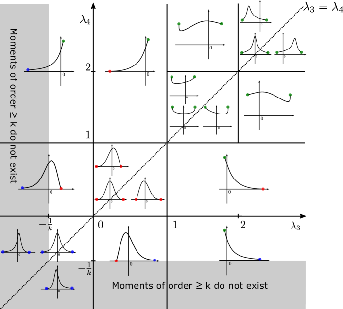
Figure 1: A graphical illustration of the PDF of the FKML family of GLD as a function of $\lambda_{3}$ and $\lambda_{4}$. The values of $\lambda_{1}$ and $\lambda_{2}$ are set to 0 and 1, respectively. The blue points indicate that the PDF has infinite support in the marked direction. In contrast, both the red and green points denote the boundary points of the PDF support. More precisely, the PDF $f_{W}(w)=0$ on the red dots, whereas $f_{W}(w)=1$ on the green ones.

3 Polynomial chaos expansions

Consider a deterministic computational model ${\mathcal{M}}_{d}(\bm{x})$ that maps a set of input parameters $\bm{x}=\left(x_{1},x_{2},\ldots,x_{M}\right)^{T}\in{\mathcal{D}}_{\bm{X}}\subset{\mathbb{R}}^{M}$ to the system response $z\in{\mathbb{R}}$. In the context of uncertainty quantification, the input variables are affected by uncertainty due to lack of knowledge or intrinsic variability (also called aleatory uncertainty). Therefore, they are modeled by random variables and grouped into a random vector $\bm{X}$ characterized by a joint PDF $f_{\bm{X}}$. The uncertainty in the input variables propagates through the the model ${\mathcal{M}}_{d}$ to the output, which becomes a random variable denoted by $Z={\mathcal{M}}_{d}(\bm{X})$.

Remark.

$f_{\bm{X}}$ is the joint PDF for the input variables, which is needed to define orthogonal polynomials as described below. It should not be confused with the stochasticity of the simulator addressed in the next sections.

Provided that the output random variable $Z$ has finite variance, ${\mathcal{M}}_{d}$ belongs to the Hilbert space ${\mathcal{H}}$ of square-integrable functions associated with the inner product

$$\langle u,v\rangle_{{\mathcal{H}}}\stackrel{{\scriptstyle\text{def}}}{{=}}{\mathbb{E}}\left[u(\bm{X})v(\bm{X})\right]=\int_{{\mathcal{D}}_{\bm{X}}}u(\bm{x})v(\bm{x})f_{\bm{X}}(\bm{x})\mathrm{d}\bm{x}.$$ (7)

If the joint PDF $f_{\bm{X}}$ fulfills certain conditions [19], the space spanned by multivariate polynomials is dense in ${\mathcal{H}}$. In other words, ${\mathcal{H}}$ is a separable Hilbert space admitting a polynomial basis.

In this study, we assume that $\bm{X}$ has mutually independent components, and thus the joint distribution $f_{\bm{X}}$ is expressed as

$$f_{\bm{X}}(\bm{x})=\prod_{j=1}^{M}f_{X_{j}}(x_{j}).$$ (8)

Let $\{\phi^{(j)}_{k}:k\in{\mathbb{N}}\}$ be the orthogonal polynomial basis with respect to the marginal distribution of $f_{X_{j}}$, i.e.,

$${\mathbb{E}}\left[\phi^{(j)}_{k}(X_{j})\,\phi^{(j)}_{l}(X_{j})\right]=\delta_{kl},$$ (9)

with $\delta$ being the Kronecker symbol defined by $\delta_{kl}=1$ if $k=l$ and $\delta_{kl}=0$ otherwise. Then, the multivariate orthogonal polynomial basis can be obtained as the tensor product of univariate polynomials [20]:

$$\psi_{\bm{\alpha}}(\bm{x})=\prod_{j=1}^{M}\phi^{(j)}_{\alpha_{j}}(x_{j}),$$ (10)

where $\bm{\alpha}=\left(\alpha_{1},\ldots,\alpha_{M}\right)\in{\mathbb{R}}^{M}$ denotes the multi-index of degrees. Each component $\alpha_{j}$ indicates the polynomial degree of $\phi_{\alpha_{j}}$ and thus of $\psi_{\bm{\alpha}}$ in the $j$th variable $x_{j}$. For some classical distributions, e.g., normal, uniform, exponential, the associated univariate orthogonal polynomials are well known as Hermite, Legendre, and Laguerre polynomials [21]. For arbitrary marginal distributions, such a basis can be computed numerically through the Stieltjes procedure [22].

Following the construction defined in Eq. 10, $\left\{\psi_{\bm{\alpha}}(\cdot),\bm{\alpha}\in{\mathbb{N}}^{M}\right\}$ forms an orthogonal basis for ${\mathcal{H}}$. Thus, the random output $Z$ can be represented by

$$Z={\mathcal{M}}_{d}(\bm{X})=\sum_{\bm{\alpha}\in{\mathbb{N}}^{M}}c_{\bm{\alpha}}\psi_{\bm{\alpha}}(\bm{X}),$$ (11)

where $c_{\bm{\alpha}}$ is the coefficient associated with the basis function $\psi_{\bm{\alpha}}$. The spectral representation in Eq. 11 is a series with infinitely many terms. In practice, it is necessary to adopt truncation schemes to approximate ${\mathcal{M}}_{d}(\bm{x})$ with a finite series defined by a finite subset ${\mathcal{A}}\subset{\mathbb{N}}^{M}$ of multi-indices. A typical scheme is the hyperbolic ($q$-norm) truncation scheme [23]:

$${\mathcal{A}}^{p,q,M}=\left\{\bm{\alpha}\in{\mathbb{N}}^{M},\|\bm{\alpha}\|_{q}=\left(\sum_{i=1}^{M}\left\lvert\alpha_{i}\right\rvert^{q}\right)^{\frac{1}{q}}\leq p\right\},$$ (12)

where $p$ is the maximum total degree of polynomials, and $q\leq 1$ defines the quasi-norm $\left\lVert\cdot\right\rVert_{q}$. Note that with $q=1$, we obtain the so-called full basis of total degree less than $p$.

For an arbitrary distribution $f_{\bm{X}}$ with dependent components of $\bm{X}$, the usual practice is to transform $\bm{X}$ into an auxiliary vector $\bm{\xi}$ with independent components (e.g., a standard normal vector) using the Nataf or Rosenblatt transform [24]. Alternatively, polynomials orthogonal to the joint distribution may be computed on the fly using a numerical Gram–Schmidt orthogonalization [25].

4 Generalized lambda models (GLaM)

4.1 Introduction

Because of their flexibility, we assume that the response random variable of a stochastic simulator for a given input vector $\bm{x}$ follows a GLD. Hence, the distribution parameters $\bm{\lambda}$ are functions of the input variables:

$$Y(\bm{x})\sim{\rm GLD}\left(\lambda_{1}(\bm{x}),\lambda_{2}(\bm{x}),\lambda_{3}(\bm{x}),\lambda_{4}(\bm{x})\right).$$ (13)

Under appropriate conditions discussed in Section 3, each component of $\bm{\lambda}(\bm{x})$ admits a spectral representation in terms of orthogonal polynomials. Recall that $\lambda_{2}(\bm{x})$ is required to be positive (see Section 2). Thus, we choose to build the associated PCE on the natural logarithm transform $\log\left(\lambda_{2}(\bm{x})\right)$. This results in the following approximations:

$$\lambda_{l}\left(\bm{x}\right) \approx\lambda^{\operatorname*{PC}}_{l}\left(\bm{x};\bm{c}\right)=\sum_{\bm{\alpha}\in{\mathcal{A}}_{l}}c_{l,\bm{\alpha}}\psi_{\bm{\alpha}}(\bm{x}),\quad l=1,3,4,$$ (14)

$$\lambda_{2}\left(\bm{x}\right) \approx\lambda^{\operatorname*{PC}}_{2}\left(\bm{x};\bm{c}\right)=\exp\left(\sum_{\bm{\alpha}\in{\mathcal{A}}_{2}}c_{2,\bm{\alpha}}\psi_{\bm{\alpha}}(\bm{x})\right),$$ (15)

where $\bm{{\mathcal{A}}}=\left\{{\mathcal{A}}_{l}:l=1,\ldots,4\right\}$ are the truncation sets defining the basis functions, and $\bm{c}=\left\{c_{l,\bm{\alpha}}:l=1,\ldots,4,\,\bm{\alpha}\in{\mathcal{A}}_{l}\right\}$ are coefficients associated to the bases. For the purpose of clarity, we explicitly express $\bm{c}$ in the spectral approximations as in $\bm{\lambda}^{\operatorname*{PC}}\left(\bm{x};\bm{c}\right)$ to emphasize that $\bm{c}$ are the model parameters.

The generalized lambda model presented above is a statistical model. It involves two approximations. First, the response distribution of a stochastic simulator is approximated by GLDs. As illustrated in Figure 1, GLDs cover a wide range of unimodal shapes but cannot produce multimodal distributions. Thus, the GLD representation is appropriate when the response distribution stays unimodal. In this case, the flexibility of GLDs allows capturing the possible shape variation of the response distribution within a single parametric family. Second, the distribution parameters $\bm{\lambda}(\bm{x})$ seen as functions of $\bm{x}$ are represented by truncated polynomial chaos expansions. So they must belong to the Hilbert space of square-integrable functions with respect to $f_{\bm{X}}(\bm{x})\,\mathrm{d}\bm{x}$.

4.2 Estimation of the model parameters

Given the truncation sets $\bm{{\mathcal{A}}}$, the coefficients $\bm{c}$ need to be estimated from data to build the surrogate model. In this paper, as opposed to [10] and the vast majority of the literature on stochastic simulators, the simulator is required to be evaluated only once on the experimental design ${\mathcal{X}}=\left\{\bm{x}^{(1)},\ldots,\bm{x}^{(N)}\right\}$, and the associated model responses are collected in ${\mathcal{Y}}=\left\{y^{(1)},\ldots,y^{(N)}\right\}$. To develop surrogate models in a nonintrusive manner, we propose using the maximum conditional likelihood estimator:

$$\hat{\bm{c}}=\arg\max_{\bm{c}\in{\mathcal{C}}}\,\mathsf{L}\left(\bm{c}\right),$$ (16)

where

$$\mathsf{L}\left(\bm{c}\right)=\sum_{i=1}^{N}\log\left(f^{{\rm GLD}}\left(y^{(i)};\bm{\lambda}^{\operatorname*{PC}}\left(\bm{x}^{(i)};\bm{c}\right)\right)\right).$$ (17)

Here, $f^{{\rm GLD}}$ denotes the PDF of the GLD defined in Eq. 3, and ${\mathcal{C}}$ is the search space for $\bm{c}$. The estimator introduced in Eq. 17 can be derived from minimizing the Kullback–Leibler divergence between the surrogate PDF and the underlying true response PDF over ${\mathcal{D}}_{\bm{X}}$; see details in [10]. The advantages of this estimation method are twofold. On the one hand, it removes the need for replications in the experimental design. On the other hand, if a GLaM for a certain choice of $\bm{c}$ can exactly represent the stochastic simulator, the proposed estimator is consistent under mild conditions, as shown in Theorem 1 (see Section A.1 for a detailed proof).

Theorem 1.

Let $(\bm{X}^{(1)},Y^{(1)}),\ldots,(\bm{X}^{(N)},Y^{(N)})$ be independent and identically distributed random variables following $\bm{X}\sim P_{\bm{X}}$ and $Y(\bm{x})\sim{\rm GLD}\left(\bm{\lambda}^{\operatorname*{PC}}(\bm{x};\bm{c}_{0})\right)$. If the following conditions are fulfilled, the estimator defined in Eq. 16 is consistent, that is,

$$\hat{\bm{c}}\xrightarrow{\text{a.s.}}\bm{c}_{0}.$$ (18)

1. $P_{\bm{X}}$ is absolutely continuous with respect to the Lebesgue measure of ${\mathbb{R}}^{M}$, i.e., the joint PDF $f_{X}(\bm{x})$ is Lebesgue-measurable.

2. $f_{X}$ has a compact support ${\mathcal{D}}_{\bm{X}}$.

3. ${\mathcal{C}}$ is compact, and $\bm{c}_{0}\in{\mathcal{C}}$.

4. There exists a set $A\subset{\mathcal{D}}_{\bm{X}}$ with $P_{\bm{X}}\left(\bm{X}\in A\right)>0$ such that $\forall\bm{x}\in A$, $Y(\bm{x})$ does not follow a uniform distribution.

Most of the assumptions in the Theorem 1 are realistic, except the one that the true model can be exactly represented by a GLaM, which is rather technical to guarantee the consistency. In practice, we do not require the QoI for any input parameters following a GLD but assume that the response distribution can be well approximated by GLDs.

It is worth remarking that since a GLD can have very fat tails (see Section 2.2), solving the optimization problem may produce response PDFs with unexpected infinite moments when the model is trained on a small data set. To prevent too-fat tails (if no prior knowledge suggests it), we apply the threshold $\lambda^{\operatorname*{PC}}_{3}(\bm{x})=\max\left\{\lambda^{\operatorname*{PC}}_{3}(\bm{x};\hat{\bm{c}}),-0.3\right\}$ and $\lambda^{\operatorname*{PC}}_{4}(\bm{x})=\max\left\{\lambda^{\operatorname*{PC}}_{4}(\bm{x};\hat{\bm{c}}),-0.3\right\}$, which indicates that we enforce the surrogate PDFs to have finite moments up to order $3$ (higher order moments may exist depending on $\hat{\bm{c}}$). Thresholds larger than $-0.3$ (e.g., from $-0.1$ to $0$) can be used if the response PDF is known to be light-tailed. Note that when enough data are available, these operations are unnecessary because the resulting model does not exceed the threshold. Although the thresholdings could have been imposed in the model definition in Eq. 14, they change the regularity of the optimization problem, and do not generally improve the performance according to our experience. Therefore, we only use them for postprocessing.

Remark 1.

While we consider the simulator to be evaluated only once for each point of the experimental design in this paper, the estimator defined in Eq. 16 is not limited to this type of data. When replications are available, the objective function can be reformulated to

$$\mathsf{L}\left(\bm{c}\right)=\sum_{i=1}^{N}\frac{1}{R^{(i)}}\sum_{r=1}^{R^{(i)}}\log\left(f^{{\rm GLD}}\left(y^{(i,r)};\bm{\lambda}^{\operatorname*{PC}}\left(\bm{x}^{(i)};\bm{c}\right)\right)\right),$$ (19)

where $R^{(i)}$ denotes the number of replications at point $\bm{x}^{(i)}$, and $y^{(i,r)}$ is the model response for $\bm{x}^{(i)}$ at the $r$th replication. In addition, if $R^{(i)}$ is constant for all points $\bm{x}^{(i)}\in{\mathcal{X}}$, Eq. 19 provides the same estimator as in our previous work [10].

4.3 Fitting procedure

In practice, the evaluation of $\mathsf{L}(\bm{c})$ is not straightforward because the PDF of GLDs does not have an explicit form as shown in Eq. 3. Details about the evaluation procedure are given in [10]. Note that the optimization problem Eq. 16 is subject to complex inequality constraints due to the dependence of the PDF support on $\bm{\lambda}$ (see Eq. 4). Given a starting point, we follow the optimization strategy developed in [10]: We first apply the derivative-based trust-region optimization algorithm [26] without constraints. If none of the inequality constraints is activated at the optimum, we keep the results as the final estimates. Otherwise, the constrained (1+1)-CMA-ES algorithm [27] available in the software UQLab [28] is used instead.

Because $\mathsf{L}(\bm{c})$ is highly nonlinear, a good starting point is necessary to guarantee the convergence of the optimization algorithm. In this section, we introduce a robust method to find a suitable starting point.

According to Eq. 5, the mean $\mu(\bm{x})$ and the variance function $v(\bm{x})$ of a GLaM satisfy

$$\begin{split}\mu(\bm{x})&=\lambda^{\operatorname*{PC}}_{1}(\bm{x})+\frac{1}{\lambda^{\operatorname*{PC}}_{2}(\bm{x})}g\left(\lambda^{\operatorname*{PC}}_{3}(\bm{x}),\lambda^{\operatorname*{PC}}_{4}(\bm{x})\right),\\ \log\left(v(\bm{x})\right)&=-2\log\left(\lambda^{\operatorname*{PC}}_{2}(\bm{x})\right)+h\left(\lambda^{\operatorname*{PC}}_{3}(\bm{x}),\lambda^{\operatorname*{PC}}_{4}(\bm{x})\right),\end{split}$$ (20)

where we group the dependence of $\mu$ and $\log(v)$ on $\lambda_{3}$ and $\lambda_{4}$ into $g$ and $h$, respectively, for the purpose of simplicity. If $\lambda^{\operatorname*{PC}}_{3}(\bm{x})$ and $\lambda^{\operatorname*{PC}}_{4}(\bm{x})$ do not vary strongly on ${\mathcal{D}}_{\bm{X}}$, we observe that the variations of the mean and the variance function are mostly dominated by the location parameter $\lambda^{\operatorname*{PC}}_{1}(\bm{x})$ and the scale parameter $\lambda^{\operatorname*{PC}}_{2}(\bm{x})$.

Recall that the spectral approximation for $\lambda_{2}(\bm{x})$ is on its logarithmic transform. If a PCE can be constructed for $\mu(\bm{x})$ and $-\frac{1}{2}\log\left(v(\bm{x})\right)$, the associated coefficients can be used as a preliminary guess for the coefficients of $\lambda^{\operatorname*{PC}}_{1}(\bm{x})$ and $\lambda^{\operatorname*{PC}}_{2}(\bm{x})$, respectively. As a result, we first focus on estimating the mean and the variance function as follows:

$$\mu(\bm{x})=\sum_{\bm{\alpha}\in{\mathcal{A}}_{\mu}}c_{\mu,\bm{\alpha}}\psi_{\bm{\alpha}}(\bm{x}),\quad v(\bm{x})=\exp\left(\sum_{\bm{\alpha}\in{\mathcal{A}}_{v}}c_{v,\bm{\alpha}}\psi_{\bm{\alpha}}(\bm{x})\right),$$

where the form of the variance function implies a multiplicative heteroskedastic effect (see [29]).

The mean estimation is a classical regression problem. However, since the variance function is also unknown and needs to be estimated, the heteroskedastic effect should be taken into account. Many methods have been developed in statistics and applied science to tackle heteroskedastic regression problems. They can be classified into two groups: one class of methods relies on repeated measurements at given input values [30, 31, 32] (replication-based), whereas a second class of methods jointly estimates both quantities by optimizing certain functions without the need for replications [33, 34, 35, 36]. Some studies [34, 36] have shown higher efficiency of the second class of methods over the former. This finding supports our pursuit for a replication-free approach. In particular, we opt for feasible generalized least-squares (FGLS) [37], which iteratively fits the mean and variance functions in an alternative way.

The details are described in Algorithm 1. In this algorithm, $\operatorname{OLS}$ denotes the use of ordinary least-squares, and $\operatorname{WLS}$ is weighted least-squares. $\hat{\bm{v}}$ corresponds to the set of estimated variances on the design points in ${\mathcal{X}}$ which are then used as weights in $\operatorname{WLS}$ to re-estimate $\bm{c}_{\mu}$.

Algorithm 1 Feasible generalized least-squares (FGLS)

1:  $\hat{\bm{c}}_{\mu}\leftarrow\operatorname{OLS}\left({\mathcal{X}},{\mathcal{Y}}\right)$

2:  for $i\leftarrow 1,\ldots,N_{\rm FGLS}$ do

3:     $\hat{\bm{\mu}}\leftarrow\sum_{\bm{\alpha}\in{\mathcal{A}}_{\mu}}c_{\mu,\bm{\alpha}}\psi_{\bm{\alpha}}({\mathcal{X}})$

4:     $\tilde{\bm{r}}\leftarrow 2\log\left(\left\lvert{\mathcal{Y}}-\hat{\bm{\mu}}\right\rvert\right)$

5:     $\hat{\bm{c}}_{v}\leftarrow\operatorname{OLS}\left({\mathcal{X}},\tilde{\bm{r}}\right)$

6:     $\hat{\bm{v}}=\exp\left(\sum_{\bm{\alpha}\in{\mathcal{A}}_{v}}c_{v,\bm{\alpha}}\psi_{\bm{\alpha}}({\mathcal{X}})\right)$

7:     $\hat{\bm{c}}_{\mu}\leftarrow\operatorname{WLS}\left({\mathcal{X}},{\mathcal{Y}},\hat{\bm{v}}\right)$

8:  end for

9:  Output: $\hat{\bm{c}}_{\mu}$, $\hat{\bm{c}}_{v}$

After obtaining $\hat{\bm{c}}_{\mu}$ and $\hat{\bm{c}}_{v}$ from FGLS, we perform two rounds of the optimization procedure described at the beginning of this section to build the GLaM surrogate. First, we set the starting points as $\bm{c}_{1}=\bm{c}_{\mu}$, $\bm{c}_{2}=-\frac{1}{2}\bm{c}_{v}$, and $\lambda^{\operatorname*{PC}}_{3}(\bm{x})=\lambda^{\operatorname*{PC}}_{4}(\bm{x})=0.13$, which corresponds to a normal-like shape. Then, we fit a GLaM with $\lambda^{\operatorname*{PC}}_{3}(\bm{x})$ $\lambda^{\operatorname*{PC}}_{4}(\bm{x})$ being only constant; i.e., the coefficients of nonconstant basis functions are kept as zeros during the fitting. Finally, we use the resulting estimates as a starting point and construct a final GLaM with all the considered basis functions by solving Eq. 17.

4.4 Truncation schemes

Provided that the bases of $\bm{\lambda}^{\operatorname*{PC}}(\bm{x})$ are given, we have presented a procedure to construct GLaMs from data in the previous section. However, there is generally no prior knowledge that would help select the truncation sets ${\mathcal{A}}_{l}$’s ab initio. In this section, we develop a method to determine a suitable hyperbolic truncation scheme ${\mathcal{A}}^{p,q,M}$ presented in Eq. 12 for each component of $\bm{\lambda}^{\operatorname*{PC}}(\bm{x})$.

As discussed in Section 2, $\lambda^{\operatorname*{PC}}_{3}(\bm{x})$ and $\lambda^{\operatorname*{PC}}_{4}(\bm{x})$ control the shape variations of the response PDF. We assume that the shape does not vary in a strongly nonlinear way. Hence, the associated $p$ can be set to a small value, e.g., $p=1$, in practice. In contrast, $\lambda^{\operatorname*{PC}}_{1}(\bm{x})$ and $\lambda^{\operatorname*{PC}}_{2}(\bm{x})$ require possibly larger degree $p$ since their behavior is associated with the mean and the variance function, which might vary nonlinearly over ${\mathcal{D}}_{\bm{X}}$. To this end, we modify Algorithm 1 to adaptively find appropriate truncation schemes for $\mu(\bm{x})$ and $v(\bm{x})$, which are then used for $\lambda_{1}(\bm{x})$ and $\lambda_{2}(\bm{x})$, respectively.

Algorithm 2 Modified feasible generalized least-squares

1:  Input: $\left({\mathcal{X}},{\mathcal{Y}}\right)$, $\bm{p}_{1}$, $\bm{q}_{1}$, $\bm{p}_{2}$, $\bm{q}_{2}$

2:  ${\mathcal{A}}_{\mu},\,\,\hat{\bm{c}}_{\mu}\leftarrow\operatorname{AOLS}\left({\mathcal{X}},{\mathcal{Y}},\bm{p}_{1},\bm{q}_{1}\right)$

3:  for $i\leftarrow 1,\ldots,N_{\rm FGLS}$ do

4:     $\hat{\bm{\mu}}\leftarrow\sum_{\bm{\alpha}\in{\mathcal{A}}_{\mu}}c_{m,\bm{\alpha}}\psi_{\bm{\alpha}}({\mathcal{X}})$

5:     $\tilde{\bm{r}}\leftarrow 2\log\left(\left\lvert{\mathcal{Y}}-\hat{\bm{\mu}}\right\rvert\right)$

6:     ${\mathcal{A}}^{i}_{v},\,\,\hat{\bm{c}}^{i}_{v},\,\,\varepsilon^{i}_{\rm LOO}\leftarrow\operatorname{AOLS}\left({\mathcal{X}},\tilde{\bm{r}},\bm{p}_{2},\bm{q}_{2}\right)$

7:     $\hat{\bm{v}}\leftarrow\exp\left(\sum_{\bm{\alpha}\in{\mathcal{A}}_{v}}c_{v,\bm{\alpha}}\psi_{\bm{\alpha}}({\mathcal{X}})\right)$

8:     $\hat{\bm{c}}_{\mu}\leftarrow\operatorname{WLS}\left({\mathcal{X}},{\mathcal{Y}},{\mathcal{A}}_{\mu},\hat{\bm{v}}\right)$

9:  end for

10:  $i^{*}=\arg\min\left\{\varepsilon^{i}_{\rm LOO}:i=1,\ldots,N_{\rm FGLS}\right\}$

11:  Output: ${\mathcal{A}}_{\mu}$, $\hat{\bm{c}}^{i^{*}}_{\mu}$, ${\mathcal{A}}^{i^{*}}_{v}$, $\hat{\bm{c}}^{i^{*}}_{v}$

Algorithm 2 presents the modified FGLS. Instead of using OLS, we apply the adaptive ordinary least-squares with degree and $q$-norm adaptivity (referred to as $\operatorname{AOLS}$) [38]. This algorithm builds a series of PCEs, each of which is obtained by applying OLS with the truncation set ${\mathcal{A}}^{p,q,M}$ defined by a particular combination of $p\in\bm{p}$ and $q\in\bm{q}$. Then, it selects the truncation scheme for which the associated PCE has the lowest leave-one-out error. In the modified FGLS, the truncation set ${\mathcal{A}}_{\mu}$ for $\mu(\bm{x})$ is selected only once (before the loop), whereas several truncation schemes $\left\{{\mathcal{A}}^{i}_{v}:i=1,\ldots,N_{\rm FGLS}\right\}$ are obtained. We select the one corresponding to the smallest leave-one-out error on the expansion of the variance as the truncation set ${\mathcal{A}}_{v}$ for $v(\bm{x})$. After running Algorithm 2, we apply the two-round optimization strategy described in the previous section to build the GLaM corresponding to the selected truncation schemes.

There are several parameters to be determined in Algorithm 2. In the following examples and applications, we set the candidate degrees $\bm{p}_{1}=\left\{0,\ldots,10\right\}$ for $\lambda^{\operatorname*{PC}}_{1}(\bm{x})$, and $\bm{p}_{2}=\left\{0,\ldots,5\right\}$ for $\lambda^{\operatorname*{PC}}_{2}(\bm{x})$. $\bm{p}_{1}$ contains high degrees to approximate possibly highly nonlinear mean functions, the accuracy of which is crucial for basis selections for $\lambda_{2}(\bm{x})$ in Algorithm 2. $\bm{p}_{2}$ is set to have degrees up to 5, allowing relatively complex variations. The lists of $q$-norms are $\bm{q}_{1}=\bm{q}_{2}=\left\{0.4,0.5,0.6,0.7,0.8,0.9,1\right\}$, which contains the full basis. The total number of FGLS iterations is set to $N_{\rm FGLS}=10$ which, according to our experience, is enough to find an appropriate truncated set for $\lambda^{\operatorname*{PC}}_{2}(\bm{x})$.

5 Application examples

In this section, we validate the proposed algorithm on two analytical examples and two case studies in mathematical finance and epidemiology. In the four cases, the response distributions do not belong to a single parametric family, so as to test the flexibility of the proposed method. In addition, we compare the performance of GLaMs with the nonparametric kernel conditional density estimator from the package np [39] implemented in R. The latter performs a thorough leave-one-out cross-validation with a multistart strategy to choose the bandwidths [14], which is one of the state-of-the-art kernel estimation methods. The surrogate model built by this method is referred to as the kernel conditional density estimator (KCDE).

Alongside GLaM and KCDE, another surrogate model, the heteroskedastic Gaussian process (denoted by GP), is also considered. This model assumes that the response distribution is Gaussian, and the mean and variance functions are represented by Gaussian processes. We apply the method proposed by Binois et. al. [40] which adopts a sequential design strategy to actively balance the trade-off between replications and explorations. The algorithm is available in the package hetGP in R. However, due to the sequential design (the new points are added one by one), building such a surrogate can be very time-consuming (cf. Section 5.2 for details). Consequently, we present the comparisons with hetGP only for the first two examples.

Moreover, for comparison purposes, we consider another “Gaussian” surrogate model where we represent the response distribution with a normal distribution. The associated mean and variance, which are functions of the input $\bm{x}$, are not fitted to data but set to the true values of the simulator. In other words, this surrogate model should represent the “oracle” of Gaussian-type mean-variance surrogate models, such as the ones presented in [36, 41].

We use Latin hypercube sampling [42] to generate the experimental design for GLaM and KCDE. The stochastic simulator is only evaluated once for each vector of input parameters. The associated QoI values are used to construct surrogate models with the proposed estimation procedure in Section 4.3. In contrast, the construction of the GP relies on a sequential design strategy which adaptively find new points to evaluate [40]. Hence, we use Latin hypercube sampling of $20\%$ of the total number of model runs to initiate the process. Then, the algorithm proceeds by iteratively looking for points to evaluate and updating the surrogate.

To quantitatively assess the performance of the surrogate model, we define an error measure between the underlying model and the emulator by

$$\varepsilon={\mathbb{E}}\left[d\left(Y(\bm{X}),\hat{Y}(\bm{X})\right)\right],$$ (21)

where $Y(\bm{X})$ is the model response, $\hat{Y}(\bm{X})$ corresponds to that of the surrogate, $d\left(Y_{1},Y_{2}\right)$ denotes the contrast measure between the probability distributions of $Y_{1}$ and $Y_{2}$, and the expectation is taken with respect to $\bm{X}$. In this study, we use the normalized Wasserstein distance, defined by

$$d\left(Y_{1},Y_{2}\right)=\frac{d_{\rm WS}\left(Y_{1},Y_{2}\right)}{\sigma\left(Y_{1}\right)},$$ (22)

where $d_{\rm WS}$ is the Wasserstein distance of order two [43] defined by

$$d_{\rm WS}\left(Y_{1},Y_{2}\right)\stackrel{{\scriptstyle\text{def}}}{{=}}\left\lVert Q_{1}-Q_{2}\right\rVert_{2}=\sqrt{\int_{0}^{1}\left(Q_{1}(u)-Q_{2}(u)\right)^{2}\mathrm{d}u}\,,$$ (23)

where $Q_{1}$ and $Q_{2}$ are the quantile functions of $Y_{1}$ and $Y_{2}$, respectively. As a summary, by combining Eq. 21 and Eq. 23 the global error reads

$$\varepsilon=\int_{{\mathcal{D}}_{\bm{X}}}\sqrt{\int_{0}^{1}\left(Q_{Y(\bm{x})}(u)-Q_{\hat{Y}(\bm{x})}(u)\right)^{2}\,\mathrm{d}u}\,\frac{f_{\bm{X}}(\bm{x})}{\sqrt{{\rm Var}\left[Y(\bm{x})\right]}}\,\mathrm{d}\bm{x}$$ (24)

Following this definition, the standard deviation $\sigma_{Y_{1}}$ can be seen as the Wasserstein distance between the distribution of $Y_{1}$ and a degenerate distribution concentrated at the mean value $\mu_{Y_{1}}$. As a result, the Wasserstein distance normalized by the standard deviation can be interpreted as the ratio of the error related to emulating the distribution of $Y_{1}$ by that of $Y_{2}$, and to using the mean value $\mu_{Y_{1}}$ as a proxy of $Y_{1}$.

Because $d_{\rm WS}$ is invariant under translation, the normalized Wasserstein distance is invariant under both translation and scaling; that is,

$$\forall a\in{\mathbb{R}}\setminus{0},b\in{\mathbb{R}}\quad\frac{d_{\text{WS}}\left(a\,Y_{1}+b,a\,Y_{2}+b\right)}{\sigma(a\,Y_{1}+b)}=\frac{d_{\text{WS}}\left(Y_{1},Y_{2}\right)}{\sigma(Y_{1})}.$$ (25)

To calculate the expectation in Eq. 21, we use Latin hypercube sampling to generate a test set ${\mathcal{X}}_{\rm test}$ of size $N_{\rm test}=1{,}000$ in the input space. The normalized Wasserstein distance is calculated for each $\bm{x}\in{\mathcal{X}}_{\rm test}$ and then averaged by $N_{\rm test}$.

For the last two case studies, the analytical response distribution of $Y(\bm{x})$ is unknown. To characterize it, we repeatedly evaluate the model $10^{4}$ times for $\bm{x}$. In addition, we also compare some summarizing statistical quantity $b(\bm{x})$ of the model response $Y(\bm{x})$, such as the mean ${\mathbb{E}}\left[Y(\bm{x})\right]$ or variance ${\rm Var}\left[Y(\bm{x})\right]$, depending on the focus of the application. Note that $b(\bm{x})$ is a deterministic function of input variables, and we define the normalized mean-squared error by

$$\varepsilon_{b}=\frac{\sum_{i=1}^{N_{\rm test}}\left(b^{(i)}_{S}-\hat{b}^{(i)}\right)^{2}}{\sum_{i=1}^{N_{\rm test}}\left(\hat{b}^{(i)}-\bar{\hat{b}}\right)^{2}},\text{ with }\bar{\hat{b}}=\frac{1}{N_{\rm test}}\sum_{i=1}^{N_{\rm test}}\hat{b}^{(i)},$$ (26)

where $b^{(i)}_{S}$ is the value predicted by the surrogate for $\bm{x}^{(i)}\in{\mathcal{X}}_{\rm test}$, and $\hat{b}^{(i)}$ denotes the quantity estimated from $10^{4}$ replicated runs of the original stochastic simulator for $\bm{x}^{(i)}$. The error $\varepsilon_{b}$ defined in Eq. 26 indicates how much of the variance of $b(\bm{X})$ cannot be explained by $b_{S}(\bm{X})$ estimated from surrogate model.

Experimental designs of various size $N\in\left\{250;500;1{,}000;2{,}000;4{,}000\right\}$ are investigated to study the convergence of the proposed method. Each scenario is run 50 times with independent experimental designs to account for statistical uncertainty in the random design for GLaM and KCDE. For GP, $N$ corresponds to the total number of model runs. We repeat 10 times for each value of $N$ (i.e., 10 heteroskedastic Gaussian processes are built using the same number of model runs). As a consequence, error estimates for each $N$ are represented by box plots.

5.1 Example 1: a two-dimensional simulator

The first example is the Black–Scholes model used for stock prices [44]:

$$\mathrm{d}S_{t}=x_{1}\,S_{t}\,\mathrm{d}t+x_{2}\,S_{t}\,\mathrm{d}W_{t},$$ (27)

where $\bm{x}=(x_{1},x_{2})^{T}$ are the input parameters, corresponding to the expected return rate and volatility of a stock, respectively. $W_{t}$ is a standard Wiener process, which represents the source of stochasticity. Equation 27 is a stochastic differential equation whose solution $S_{t}(\bm{x})$ is a stochastic process for given parameters $\bm{x}$. Note that we explicitly express $\bm{x}$ in $S_{t}(\bm{x})$ to emphasize that $\bm{x}$ are input parameters, but the stochastic equation is defined with respect to time. Without loss of generality, we set the initial condition to $S_{0}(\bm{x})=1$.

In this example, we are interested in $Y(\bm{x})=S_{1}(\bm{x})$, which corresponds to the stock value in one year i.e., $t=1$. We set $X_{1}\sim{\mathcal{U}}(0,0.1)$ and $X_{2}\sim{\mathcal{U}}(0.1,0.4)$ to represent the input uncertainty, where the ranges are selected based on parameters calibrated from real data [45].

The solution to Eq. 27 can be derived using Itô calculus [2]: $Y(\bm{x})$ follows a lognormal distribution defined by

$$Y(\bm{x})\sim{\mathcal{L}}{\mathcal{N}}\left(x_{1}-\frac{x^{2}_{2}}{2},x_{2}\right).$$ (28)

As the distribution of $Y(\bm{x})$ is known, it is not necessary to simulate the whole process $S_{t}(\bm{x})$ with time integration to evaluate $S_{1}(\bm{x})$. Instead, we can directly generate samples from the distribution defined in Eq. 28.

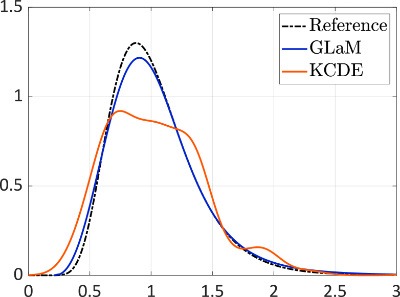
(a) PDF for $\bm{x}=(0.03,0.33)^{T}$

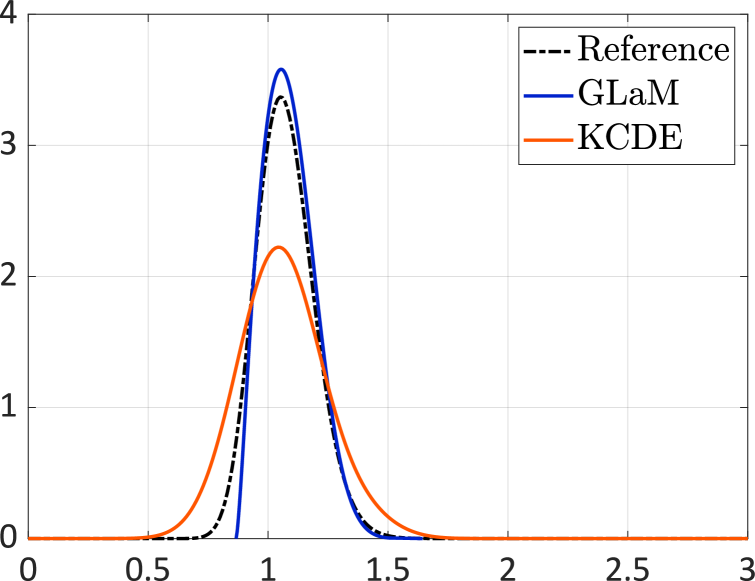
(b) PDF for $\bm{x}=(0.07,0.11)^{T}$

Figure 2: Example 1 — Comparisons of the emulated PDF, $N=500$.

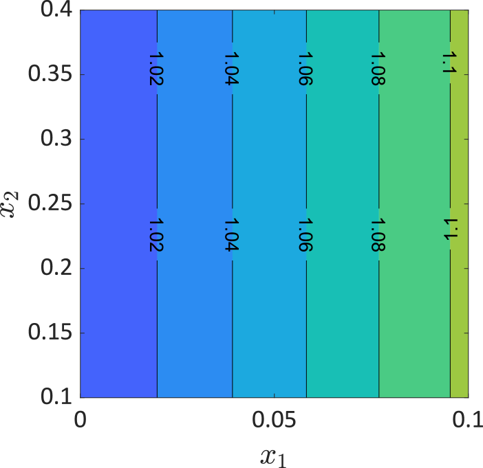
(a) Reference

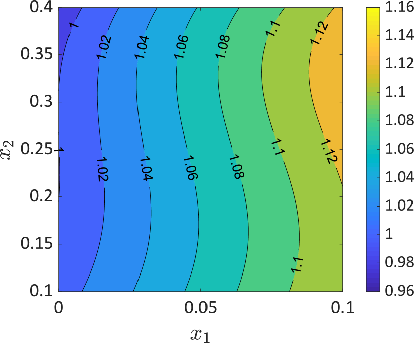
(b) GLaM

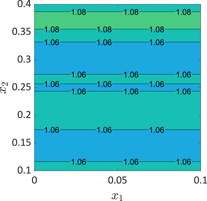
(c) KCDE

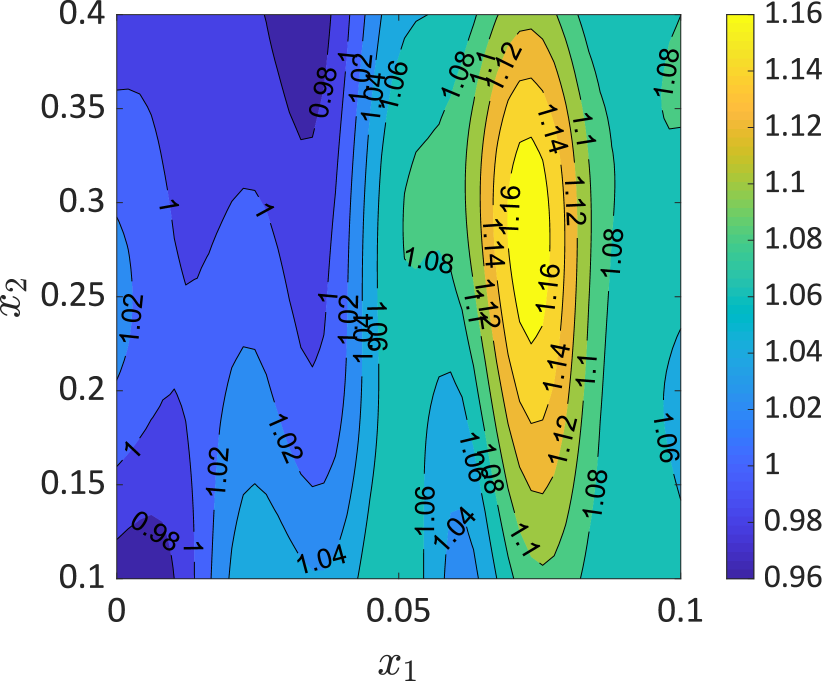
(d) GP

Figure 3: Example 1 — Comparisons of the mean function estimation, $N=500$.

(a) Reference

(b) GLaM

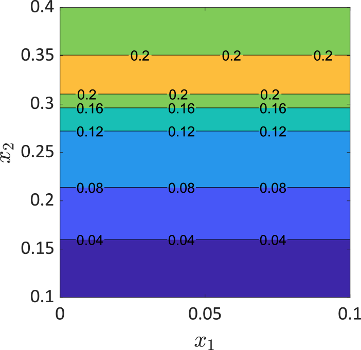
(c) KCDE

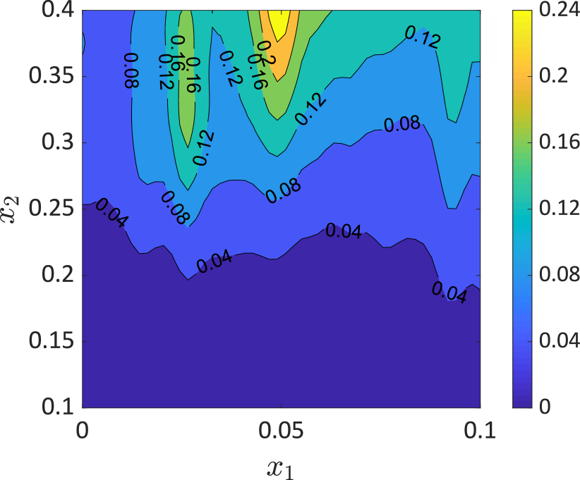
(d) GP

Figure 4: Example 1 — Comparisons of the variance function estimation, $N=500$.

Figure 2 shows two PDFs predicted by a GLaM and a KCDE built on an experimental design of size $N=500$. We observe that with $500$ model runs, the KCDE yields PDFs with spurious oscillations and demonstrates relatively poor representation of the bulk. In contrast, the GLaM can better approximate the underlying response PDF in terms of both magnitude and shape variations. Figures 3 and 4 compare the mean and variance function predicted by the GLaM, KCDE, and GP. The analytical mean function following Eq. 28 is $\exp(x_{1})$, which only depends on the first variable. The GLaM gives an accurate estimate of the mean function, whereas the KCDE captures a wrong dependence, and GP produces a rather complex structure. For the variance function, the GLaM yields a more detailed trend than the KCDE and GP.

For quantitative comparisons, Figure 5 summarizes the error measure Eq. 21 with respect to the size of experimental design. The accuracy of the oracle normal approximation is also reported (black dashed line). This error is only due to model misspecifications because we use the true mean and variance (however, the true response distribution is lognormal). The GP approach performs rather poorly and converges to the oracle normal approximation when the number of points in the experimental design increases. This means that it can accurately estimate the mean and variance functions for large data sets. However, due to the limitation of the Gaussian assumption, GP cannot further decrease the error. The average error of GLaMs built on $N=500$ model runs are smaller than that of the normal approximation. For $N>500$, GLaMs clearly provide more accurate results. KCDEs show a slow rate of convergence even in this example of dimension two. In contrast, GLaMs reveal high efficiency with a faster decrease of the errors. In terms of the average error, GLaMs outperform KCDEs for all sizes of experimental design. Furthermore, GLaMs yield an average error near $0.1$ for $N=1{,}000$, which can be hardly achieved by KCDEs even with four times more model runs.

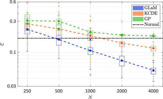
Figure 5: Example 1 — Comparison of the convergence between GLaMs and KCDEs in terms of the normalized Wasserstein distance as a function of the size of the experimental design. The dashed lines denote the average value over 50 repetitions of the full analysis. The green box plots and associated dashed lines correspond to the errors of the heteroskedastic Gaussian Process with sequential design (10 repetitions for each size of the experimental design). The black dash-dotted line represents the error of the model assuming that the response distribution is normal with the true mean and variance.

5.2 Example 2: a five-dimensional simulator

The second example is given by

$$Y(\bm{x})={\mathcal{M}}_{s}(\bm{x},\omega)=\mu(\bm{x})+\sigma(\bm{x})\cdot Z(\omega),$$ (29)

where $\bm{X}\sim{\mathcal{U}}\left([0,1]^{5}\right)$ are the input variables, and $Z\sim{\mathcal{N}}(0,1)$ is the latent variable that introduces the stochasticity. The simulator has an input dimension of $M=5$, which is used to show the performance of the proposed method in a moderate-dimensional problem. By definition, $Y(\bm{x})$ is a Gaussian random variable with mean $\mu(\bm{x})$ and standard deviation $\sigma(\bm{x})$ which are defined by

$$\begin{split}\mu(\bm{x})&=3-\sum_{j=1}^{5}j\,x_{j}+\frac{1}{5}\sum_{j=1}^{5}j\,x^{3}_{j}+\frac{1}{15}\sum_{j=1}^{5}j\,\log\left((x^{2}_{j}+x^{4}_{j})\right)+x_{1}\,x^{2}_{2}-x_{5}\,x_{3}+x_{2}\,x_{4},\\ \sigma(\bm{x})&=\exp\left(\frac{1}{10}\sum_{j=1}^{5}j\,x_{j}\right),\end{split}$$ (30)

Thus, this example has a nonlinear mean function and a strong heteroskedastic effect: the variance varies between 1 and 20.

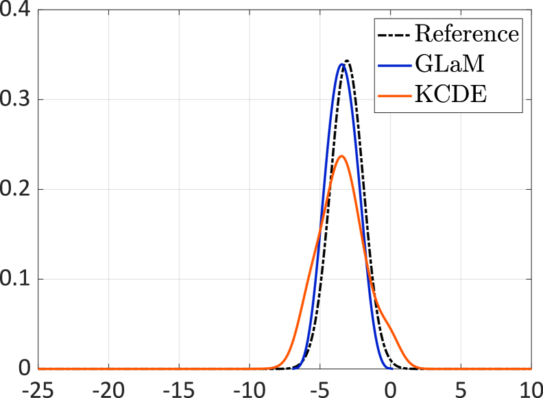
(a) PDF for $\bm{x}=(0.1,0.1,0.1,0.1,0.1)^{T}$

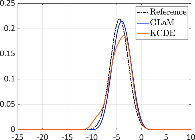
(b) PDF for $\bm{x}=(0.4,0.4,0.4,0.4,0.4)^{T}$

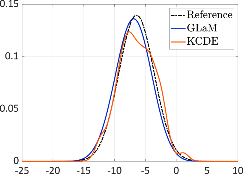
(c) PDF for $\bm{x}=(0.7,0.7,0.7,0.7,0.7)^{T}$

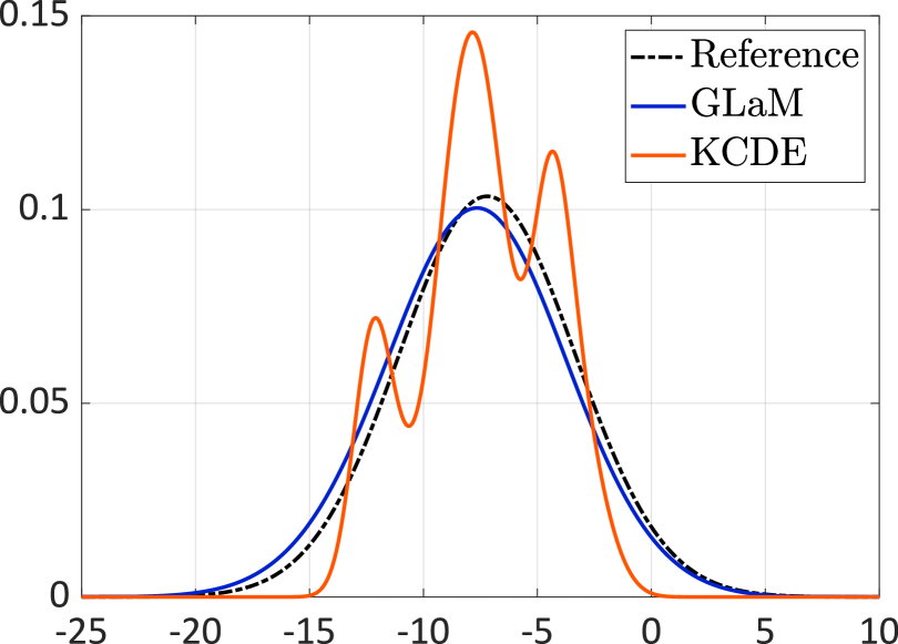
(d) PDF for $\bm{x}=(0.9,0.9,0.9,0.9,0.9)^{T}$

Figure 6: Example 2 — Comparisons of the emulated PDF, $N=1{,}000$. Variance values $1.35$, $3.32$, $8.17$, $14.88$ from (a) to (d)

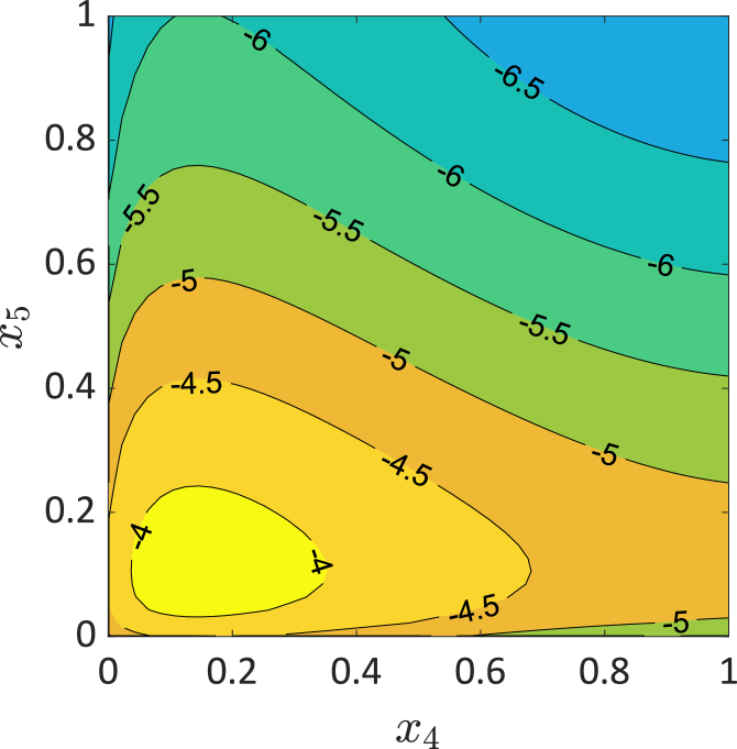
(a) Reference

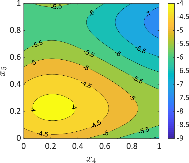
(b) GLaM

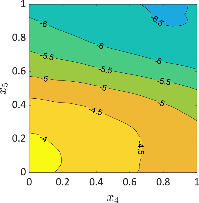
(c) KCDE

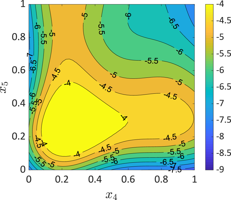
(d) GP

Figure 7: Example 2 — Comparisons of the mean function estimation in the plan $x_{4}-x_{5}$ with all the other input fixed at their expected value. The surrogate models are fitted to an ED with $N=1{,}000$.

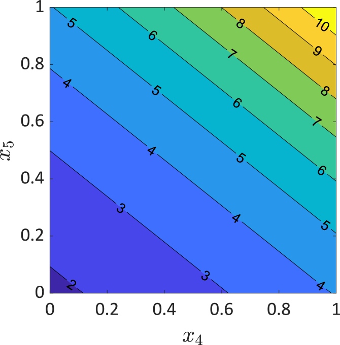
(a) Reference

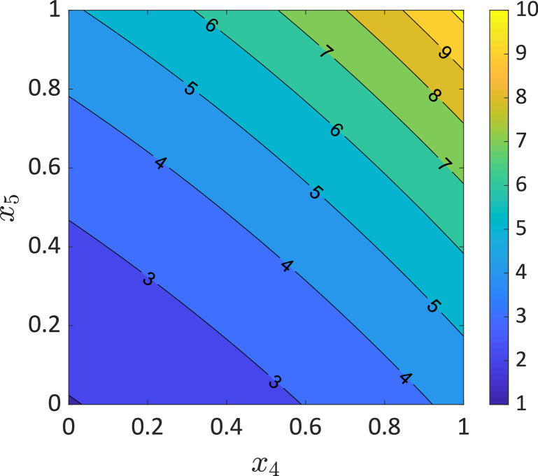
(b) GLaM

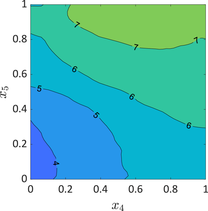
(c) KCDE

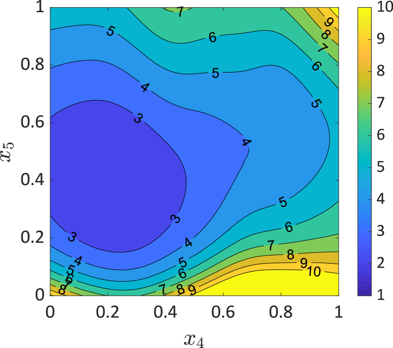
(d) GP

Figure 8: Example 2 — Comparisons of the variance function estimation in the plan $x_{4}-x_{5}$ with all the other input fixed at their expected value. The surrogate models are fitted to an ED with $N=1{,}000$.

Figure 6 compares the model response PDFs (with different variances) for four input values with those predicted by a GLaM and a KCDE built upon $1{,}000$ model runs. The results show that the GLaM correctly identifies the shape of the underlying normal distribution among all possible shapes of the GLD. Moreover, it yields a better approximation to the reference PDF, whereas KCDE tends to “wiggle” in Figure 6(d) (high variance) and overestimate the spread in Figure 6(a) (low variance). Figures 7 and 8 illustrate the mean and variance function predicted by the GLaM, KCDE, and GP in the $x_{4}-x_{5}$ plan with all the other variables fixed at their expected value. The results show that the GLaM provides more accurate estimates for both functions.

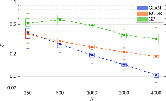
Figure 9: Example 2 — Comparison of the convergence between GLaMs and KCDEs in terms of the normalized Wasserstein distance as a function of the size of the experimental design. The dashed lines denote the average value over 50 repetitions of the full analysis. The green box plots and associated dashed lines correspond to the errors of the heteroskedastic Gaussian Process with sequential design (10 repetitions for each size of the experimental design). The “oracle” normal model has an error $\varepsilon=0$ that is not plotted here.

Similar to the first example, we perform a convergence study for $N\in\{250;\allowbreak 500;\allowbreak 1{,}000;\allowbreak 2{,}000;\allowbreak 4{,}000\}$, the results of which are shown in Fig. 9. The underlying response distribution is Gaussian, and thus the oracle normal approximation has $\varepsilon=0$, which is not reported in the figure. Surprisingly, GP gives the worst results. This may be understood as follows: the updating criterion of the sequential design targets at minimizing the integrated mean-squared error. The latter mainly focuses on improving the mean estimation (as illustrated in Figs. 7 and 8), yet both the mean and variance contribute to the Wasserstein distance Eq. 23. Also, this example is a five-dimensional problem, which results in more parameters to estimate for GP. In the case of small $N$, namely $N=250$, both the GLaMs and KCDEs perform poorly, with the GLaMs showing a similar average error but higher variability. This is explained as follows. Because of the use of $\operatorname{AOLS}$ in the modified FGLS procedure, we observe that the total number of coefficients of GLaMs to be estimated varies between 19 to 39 for $N=250$. Since the GLD is very flexible, a relatively large data set is necessary to provide enough evidence of the underlying PDF shape. Consequently, a small $N$ can lead to overfitting for high-dimensional $\bm{c}$, but good surrogates can be obtained for more parsimonious models. In contrast, KCDE always performs a thorough leave-one-out cross-validation strategy to select the bandwidths. Therefore, KCDEs show a slightly more stable estimate for $N=250$. With $N$ increasing, however, GLaMs converge much faster and outperform KCDEs for $N\geq 500$ both in terms of the mean and median of the errors. For $N\geq 1{,}000$, the average performance of GLaM is even better than the best KCDE model among the 50 repetitions.

In this example of moderate dimensionality, building a GP with sequential design is surprisingly time-consuming, especially for large experimental designs. This is probably due to the sequential design of experiments, which adds new points one by one and updates the surrogate after each enrichment. The associated simulations were performed on the ETH Euler cluster, and the average CPU time varied from 463 seconds for $N=250$ to over 9 days for $N=4{,}000$ to build a single GP. For KCDE, it took about 20 CPU seconds for $N=250$ up to $30$ minutes for $N=4{,}000$ on a standard laptop. In comparison, constructing a GLaM is always on the order of seconds: around 8 seconds for both $N=250$ and $N=4{,}000$ on a standard laptop.

5.3 Effect of replications

As pointed in Remark 1, the proposed method can also work with a data set containing replicates. The latter are simply treated as separate points in the ED. In this section, we analyze the effect of replications using the previous two analytical examples. To this end, we generate data by replicating $R\in\left\{5;10;25;50\right\}$ for each set of input parameters in the ED. We keep the total number of simulations the same as nonreplicated cases by reducing the size of the ED accordingly. For instance, a data set of total $N=1{,}000$ model evaluations with 10 replications consists of 100 different sets of input parameters, each of which is simulated 10 times.

For quantitative comparisons, we investigate a convergence study similar to Sections 5.1 and 5.2: the total number of runs $N$ varies in $\left\{250;500;1{,}000;2{,}000;4{,}000\right\}$, and each scenario is repeated 50 times.

Figures 10 and 11 summarize the error defined in Eq. 21 averaged over the 50 repetitions for each $R\in\left\{5;10;25;50\right\}$. In the first example, replications do not have a strong effect for $R\in\left\{5;10;25\right\}$. This is because the expansions for $\bm{\lambda}(\bm{x})$ contain only a few terms. Therefore, as long as we have enough ED points, exploring the input space and performing replications bring similar improvements to the surrogate accuracy. However, a large number of replications, i.e., $R=50$, gives too few ED points for small values of $N$, which yields GLaMs of poor performance.

In the second example, we observe a clear negative effect of replications: for the same total amount of model runs, the surrogate quality deteriorates when increasing the number of replications / decreasing the size of the experimental design.

In summary, homogeneous replications (i.e., those with the same number of replicates for each point of the experimental design) do not necessarily bring additional accuracy and may even lead to a “waste” of computational budget for the proposed GLaM method. Nevertheless, this does not imply that replications are always useless. On the one hand, for methods that explore the usage of replications, there is a trade-off between replications and exploration [40]. On the other hand, an adaptive selection of different numbers of replications for each point in the experimental design could possibly improve the performance of the proposed method. However, unlike the heteroskedastic GP, GLaM not only estimates the mean and the variance but also produces the whole PDF. As a result, sequential design strategies for building GLaMs remain to be developed in future study and are outside the scope of the paper.

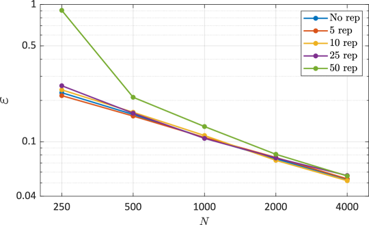
Figure 10: Example 1 — Comparison of the GLaMs built on data with different number of replications. The curves corresponds to the mean error over the 50 repetitions.

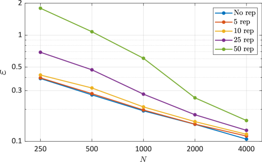
Figure 11: Example 2 — Comparison of the GLaMs built on data with different number of replications. The curves corresponds to the mean error over the 50 repetitions.

5.4 Example 3: Asian options

In this third example, we apply the proposed method to a financial case study, namely an Asian option [46]. Such an option, a.k.a. average value option, is a derivative contract, the payoff of which is contingent on the average price of the underlying asset over a certain fixed time period. Due to the path-dependent nature, an Asian option has complex behavior, and its valuation is not straightforward, as opposed to European options.

Recall the Black–Scholes model defined in Eq. 27 that represents the evolution of a stock price $S_{t}(\bm{x})$. Instead of relying on the stock price on the maturity date $t=T$, the payoff of an Asian call option reads

$$C(\bm{x})=\max\left\{A_{T}(\bm{x})-K,0\right\},\text{ with }A_{t}(\bm{x})=\frac{1}{t}\int_{0}^{t}S_{u}(\bm{x})\mathrm{d}u.$$ (31)

where $A_{t}(\bm{x})$ is called the continuous average process, and $K$ denotes the strike price. Because $A_{T}(\bm{x})$ plays an important role in the Asian option modeling Eq. 31, the PDF of $A_{T}(\bm{x})$ is of interest in this case study. As in Section 5.1, we set $T=1$, which corresponds to a one-year inspection period. We choose $X_{1}\sim{\mathcal{U}}(0,0.1)$ and $X_{2}\sim{\mathcal{U}}(0.1,0.4)$ for the two input random variables. Unlike $S_{1}(\bm{x})$, the distribution of $A_{1}(\bm{x})$ cannot be derived analytically. It is necessary to simulate the trajectory of $S_{t}(\bm{x})$ to compute $A_{1}(\bm{x})$. Based on the Markovian and lognormal properties of $S_{t}(\bm{x})$, we apply the following recursive equations for the path simulation with a time step $\Delta t=0.001$:

$$\begin{split}S_{0}(\bm{x})&=1,\\ S_{t+\Delta t}(\bm{x})\mid S_{t}(\bm{x})&\sim{\mathcal{L}}{\mathcal{N}}\left(\log\left(S_{t}(\bm{x})\right)+\left(x_{1}-\frac{x^{2}_{2}}{2}\right)\Delta t,x_{2}\sqrt{\Delta t}\right).\end{split}$$

Finally, the continuous average defined in Eq. 31 is approximated by the arithmetic mean, that is,

$$A_{1}(\bm{x})=\frac{\sum_{k=1}^{1{,}000}S_{k\Delta t}(\bm{x})}{1{,}000}$$

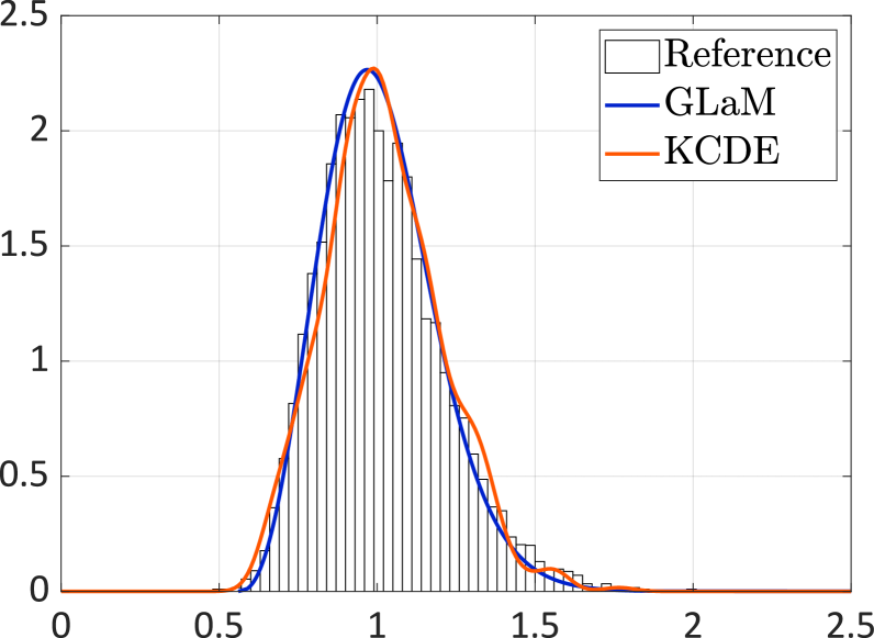
(a) PDF for $\bm{x}=(0.03,0.33)^{T}$

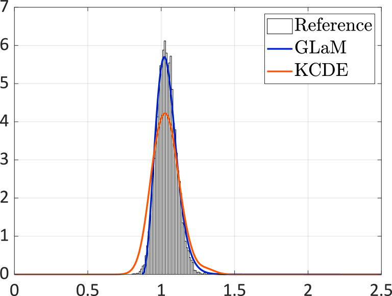
(b) PDF for $\bm{x}=(0.07,0.11)^{T}$

Figure 12: Asian option — Comparisons of the emulated PDF, $N=500$

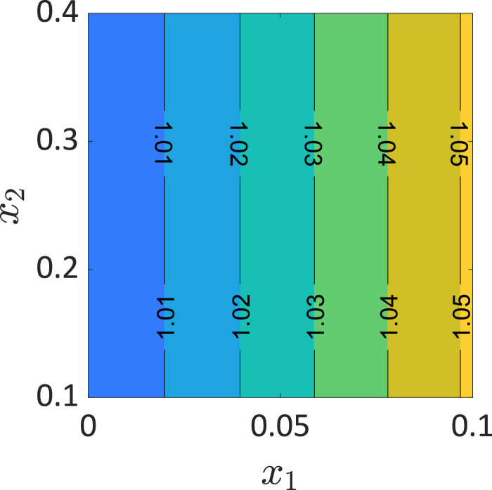
(a) Reference

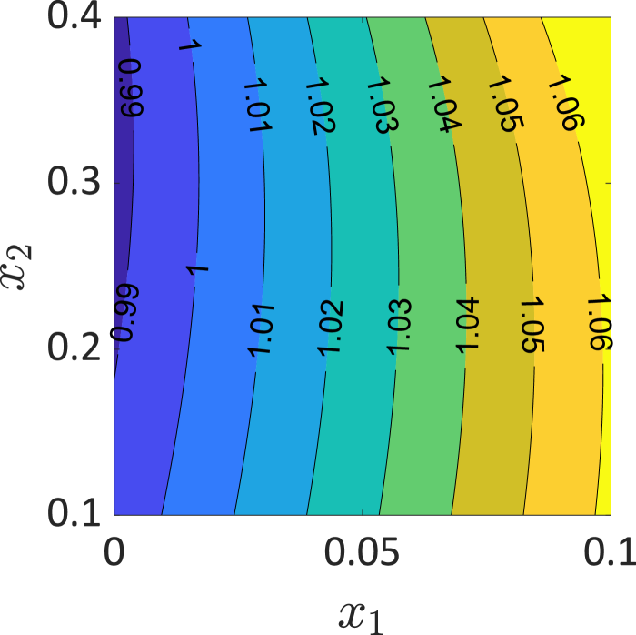
(b) GLaM

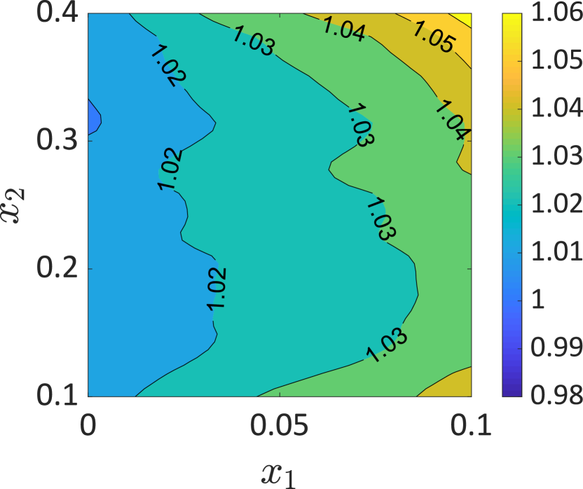
(c) KCDE

Figure 13: Asian option — Comparisons of the mean function estimation, $N=500$.

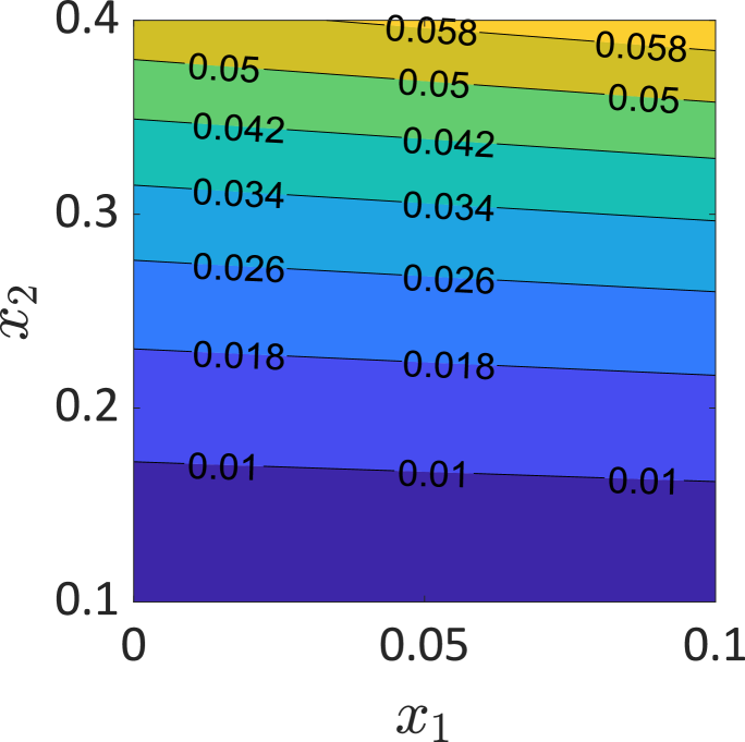
(a) Reference

(b) GLaM

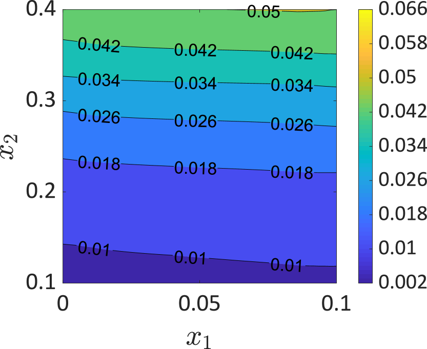
(c) KCDE

Figure 14: Asian option — Comparisons of the variance function estimation, $N=500$.

Figure 12 shows two response PDFs predicted by the two surrogate models constructed on an experimental design of $N=500$. The reference histograms are calculated from $10^{4}$ repeated runs of the simulator for each set of input parameters. We observe that the KCDE exhibits slight fluctuations at the right tail for high volatility (in Figure 12(a)) and does not well approximate the bulk of the response distribution for low volatility (in Figure 12(b)). In comparison, the GLaM can well represent the PDF shape in both cases and also more accurately approximates the tails. Figures 13 and 14 shows the mean and variance function, where the reference values can be obtained by applying Itô’s calculus. For the experimental design of $N=500$, the GLaM more accurately predicts the two functions. Finally, quantitative comparisons in Figure 15 confirm the superiority of GLaMs to KCDEs: GLaMs yield smaller average error for all $N\in\left\{250;500;1{,}000;2{,}000;4{,}000\right\}$ and demonstrate a better convergence rate. Moreover, for large experimental designs ($N\geq 2{,}000$), the average error of GLaMs is nearly half of that of KCDEs. The oracle Gaussian approximation in this case study has a similar error to GLaMs built on $1{,}000$ model runs. For $N\geq 2{,}000$, GLaMs fitted from data are much more accurate than the best possible Gaussian-type mean-variance model.

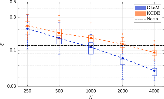
Figure 15: Asian option, average process $A_{1}(\bm{x})$ at $T=1$ year — Comparison of the convergence of GLaMs and KCDEs in terms of the normalized Wasserstein distance as a function of the size of the experimental design. The dashed lines denote the average value over $50$ repetitions of the full analysis. The black dash-dotted line represents the error of the model assuming that the response distribution is normal with the true mean and variance

As a second quantity of interest, we consider the expected payoff $\mu_{C}(\bm{x})={\mathbb{E}}\left[C(\bm{x})\right]$. This quantity not only is important for making investment decisions but also has a very similar form to the option price [46]. The definition Eq. 31 implies that the payoff $C(\bm{x})$ is a mixed random variable, which has a probability mass at $0$ and a continuous PDF on the positive line depending on the strike price $K$. In the following analysis, $K$ is set to 1.

For GLaMs, $\mu_{C}(\bm{x})$ can be calculated by

$$\mu_{C}(\bm{x})=\left(\lambda_{1}-\frac{1}{\lambda_{2}\lambda_{3}}+\frac{1}{\lambda_{2}\lambda_{4}}-K\right)\,(1-u_{K})+\frac{1}{\lambda_{2}}\,\left(\frac{1-u_{K}^{\lambda_{3}+1}}{\lambda_{3}\,\left(\lambda_{3}+1\right)}-\frac{(1-u_{K})^{\lambda_{4}+1}}{\lambda_{4}\,\left(\lambda_{4}+1\right)}\right)$$ (32)

where $\lambda$’s are the distribution parameters at $\bm{x}$, and $u_{K}$ is the solution of the nonlinear equation

$$Q(u_{K};\bm{\lambda})=K.$$ (33)

with $Q$ being the quantile function defined in Eq. 2.

Figure 16 shows the convergence of estimations of $\mu_{C}(\bm{x})$ in terms of the error defined in Eq. 26. The difference between the performance of GLaMs and KCDEs is not as significant as for the distribution estimation of $A_{1}(\bm{x})$ in Figure 15. For relatively small data sets, namely $N\leq 500$, both models work poorly: they are only able to explain on average no more than 70% of the variance of $\mu_{C}(\bm{X})$. In addition, GLaMs demonstrate a higher variability of the errors. For larger experimental designs $N\geq 2{,}000$, however, the performance of GLaMs improves significantly more than that of KCDEs. For $N=4{,}000$, the average error of GLaMs is twice smaller than that of KCDEs, and the smallest error achieved by GLaMs is one order of magnitude smaller than the best KCDE.

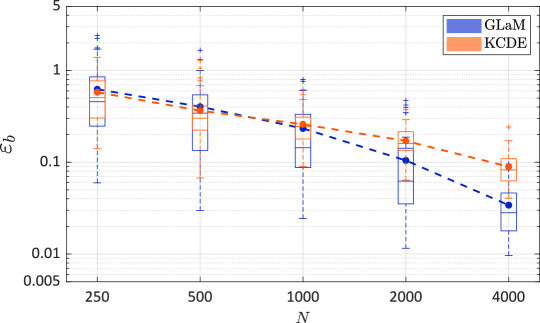
Figure 16: Asian option, expected payoff estimations — Comparison of the convergence of GLaMs and KCDEs in terms of the normalized mean squared error as a function of the size of the experimental design. The dashed lines denote the average value over $50$ repetitions of the full analysis.

5.5 Example 4: Stochastic SIR model

In this fourth example, we apply the proposed method to a stochastic susceptible-infected-recovered (SIR) model in epidemiology [3]. This model simulates the spread of an infectious disease, which can help find appropriate epidemiological interventions to minimize social and ethical impacts during the outbreak.

According to the standard SIR model, at time $t$ a population of size $P_{t}$ contains three groups of individuals: susceptible, infected, and recovered, the counts of which are denoted by $S_{t}$, $I_{t}$, and $R_{t}$, respectively. These three quantities fully characterize a population configuration at time $t$. Among the three groups, only susceptible individuals can get infected due to close contact with infected individuals, whereas an infected person can recover and becomes immune to future infections. We consider a fixed population without newborns and deaths, i.e., the total population size is constant, $P_{t}=P$. As a result, $S_{t}$, $I_{t}$, and $R_{t}$ satisfy the constraint $S_{t}+I_{t}+R_{t}=P$, and only the time evolution of $(S_{t},I_{t})$ is necessary to characterize the spread of a disease.

To account for random recoveries and interactions among individuals, stochastic SIR models are usually preferred to represent the epidemic evolution. Without going into details, the model dynamics is briefly summarized as follows. The pair $\left(I_{t},S_{t}\right)$ evolves as a continuous-time Markov process following mutual transition rates $\beta$ and $\gamma$, which denote the contact rate and recovery rate, respectively. The epidemic stops at time $t=T$ where $I_{T}=0$, indicating that no further infections can occur. The evolution process is simulated by the Gillespie algorithm [47]. The reader is referred to [3] for a more detailed presentation of stochastic SIR models.

In this case study, we set the total population equal to $P=2{,}000$ and $\beta=\gamma=0.5$ as in [41]. The initial configuration $\bm{x}=(S_{0},I_{0})$ is the vector of input parameters. To account for different scenarios, the input variables $\bm{X}$ are modeled as $X_{1}\sim{\mathcal{U}}(1200,1800)$ (initial number of susceptible individuals) and $X_{2}\sim{\mathcal{U}}(20,200)$ (initial number of infected individuals). The QoI is the total number of newly infected individuals during the outbreak, i.e., $Y(\bm{x})=S_{T}-S_{0}$.

(a) PDF for $\bm{x}=(1714,165)^{T}$

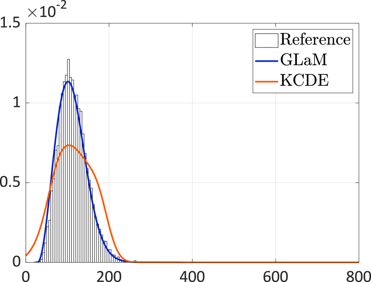
(b) PDF for $\bm{x}=(1364,61)^{T}$

Figure 17: SIR model — Comparisons of the emulated PDF, $N=500$

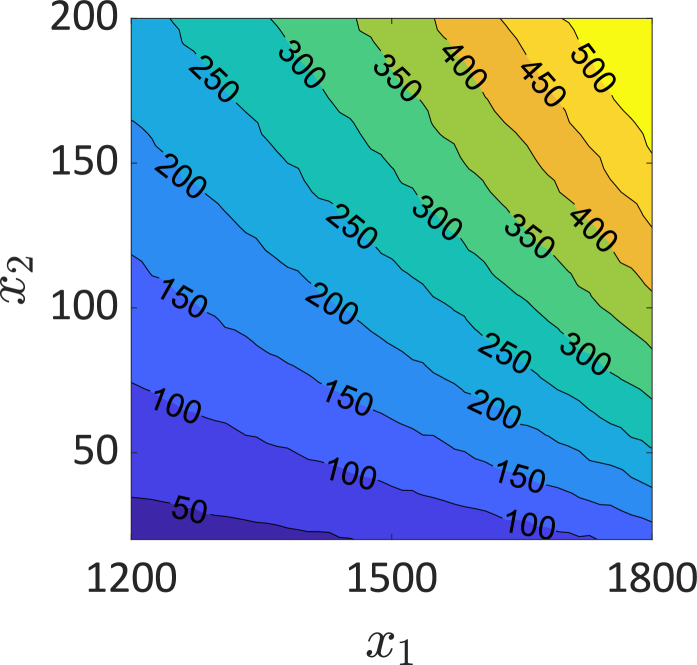
(a) Reference

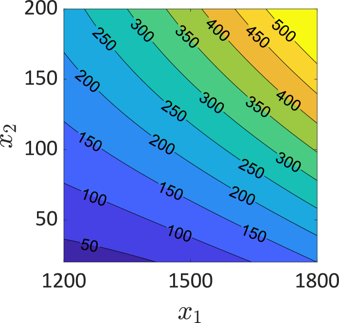
(b) GLaM

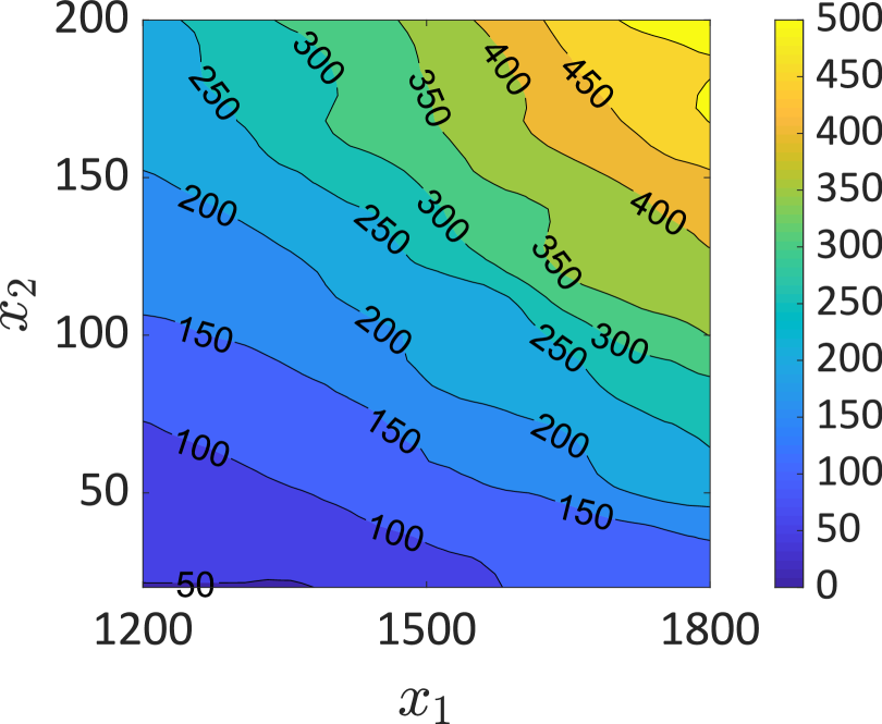
(c) KCDE

Figure 18: SIR model — Comparisons of the mean function estimation in the plan $N=500$.

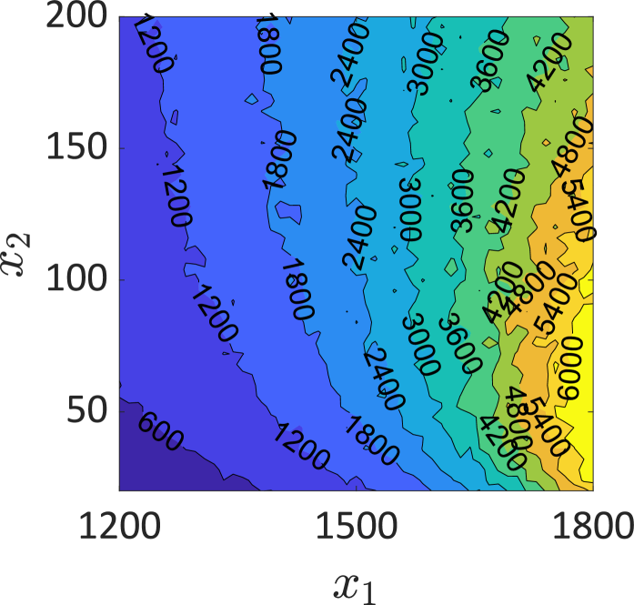
(a) Reference

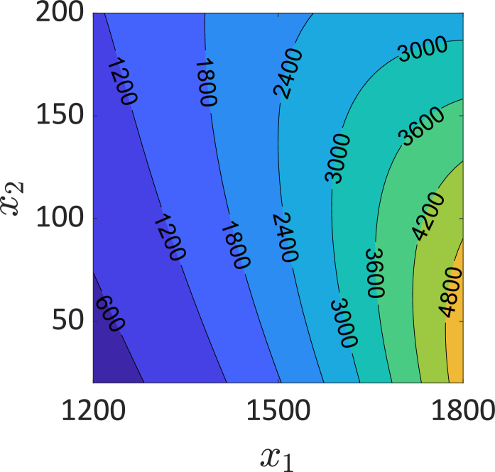
(b) GLaM

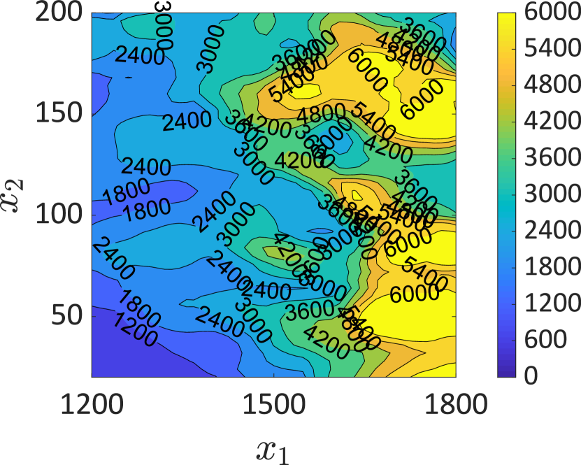
(c) KCDE

Figure 19: SIR model — Comparisons of the variance function estimation, $N=500$.

Figure 17 compares two response PDFs estimated by a GLaM and by a KCDE for two sets of initial configurations, using an experimental design of size $N=500$. The reference histograms are obtained by $10^{4}$ repeated model runs for each $\bm{x}$. We observe that the PDF shape varies: it changes from symmetric to slightly right-skewed distributions depending on the input variables. The GLaM is able to accurately capture this shape variation, while KCDE exhibits relatively poor shape representations.

Figures 18 and 19 illustrate the mean and variance function. Because the analytical results are unknown for this simulator, we use $1{,}000$ replications to estimate these quantities for plotting. We observe that both functions vary nonlinearly in the input space. Compared with the KCDE, the GLaM is able to capture the trend of the two functions and provides more accurate estimates. More detailed comparisons of the surrogate models are shown in Figure 20. The error of the oracle Gaussian approximation is quite small. This implies that the response distribution for most of the input parameters in the input space is close to a Gaussian distribution. Nevertheless, GLaMs built on $N=4{,}000$ model runs still demonstrate better average behavior. For all sizes of experimental design, GLaMs clearly outperform KCDEs. For $N\geq 500$, the biggest error of GLaMs is smaller than the smallest error of KCDEs among the 50 repetitions. Finally, to achieve the same accuracy as GLaMs, KCDEs require around 7 times more model runs.

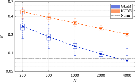
Figure 20: SIR model — Comparison of the convergence between GLaMs and KCDEs in terms of the normalized Wasserstein distance as a function of the size of the experimental design. The dashed line denotes the average value over $50$ repetitions of the full analysis. The black dash-dotted line represents the error of the model assuming that the response distribution is normal with the true mean and variance

In epidemiological management, the expected value $\mu(\bm{x})={\mathbb{E}}\left[Y(\bm{x})\right]$ is crucial for decision making [48]. Therefore, we investigate the accuracy of $\mu(\bm{x})$ estimations, and the results are in Figure 21. First, both GLaM and KCDE can explain more than 90% of the variance in $\mu(\bm{X})$ for $N=250$, which implies an overall accurate approximation to the mean function. With increasing $N$, GLaM shows a more rapid decay of the error. Furthermore, GLaMs built on $N=1{,}000$ have a similar (or even slightly better) performance to KCDEs with $N=4{,}000$.

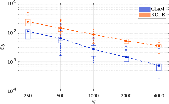
Figure 21: SIR model, mean value estimations — Comparison of the convergence between GLaMs and KCDEs in terms of the normalized mean-squared error as a function of the size of the experimental design. The dashed line denotes the average value over $50$ repetitions of the full analysis.

6 Conclusions

This paper presents an efficient and accurate nonintrusive surrogate modeling method for stochastic simulators that does not require replicated runs of the latter. We follow the setting of Zhu and Sudret [10], where the generalized lambda distribution is used to flexibly approximate the response probability density function. The distribution parameters, as functions of the input variables, are approximated by polynomial chaos expansions. In this paper, however, we do not require replicated runs of the stochastic simulator, which provides a more general and versatile approach. We propose the maximum conditional likelihood estimator to construct such a model for given basis functions. This estimation method is shown to be consistent and applicable to data with or without replications. In addition, we modify the feasible generalized least-squares algorithm to select suitable truncation schemes for the distribution parameters, which also provides a good starting point for the subsequent optimization of the likelihood function.

The performance of the new method is illustrated on analytical examples and case studies in mathematical finance and epidemics. The results show that with a reasonable number of model runs, the developed algorithm can produce surrogate models that accurately approximate the response probability density function and capture the shape variations of the latter with $\bm{x}$. Considering the normalized Wasserstein distance as an error metric, generalized lambda models always show a better convergence rate than the nonparametric kernel conditional density estimator with adaptive bandwidth selections (from the package np in R). Furthermore, the proposed method generally yields more reliable estimates of certain important quantities.

Quantifying the uncertainty of surrogate models that emulate the entire response distribution of a stochastic simulator remains to be developed in future work, especially when no or only a few replications are available. One possibility is to use cross-validation to calculate the expected loss. However, when the log-likelihood is used as the loss function such as Eq. 17, the resulting score is not intuitive and is difficult to interpret. Alternatively, with a given basis for $\bm{\lambda}(\bm{x})$ in GLaMs, one can use bootstrap [49] to assess the uncertainty in the estimation of the coefficients. Figure 22 illustrates the PDF predictions of 100 bootstrapping GLaMs of a data set with $N=500$ of Example 1. Note that the associated theoretical aspects remain to be developed: it is necessary to prove the bootstrap consistency, which is usually achieved by showing the asymptotic normality of the estimator. As a result, the asymptotic properties of the maximum likelihood estimator in Eq. 17 need to be further investigated.

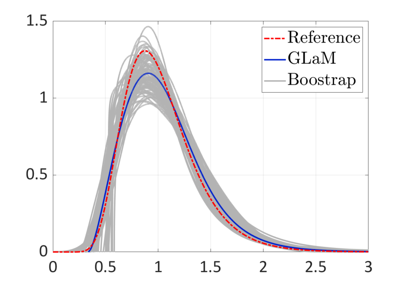
(a) PDF for $\bm{x}=(0.03,0.33)^{T}$

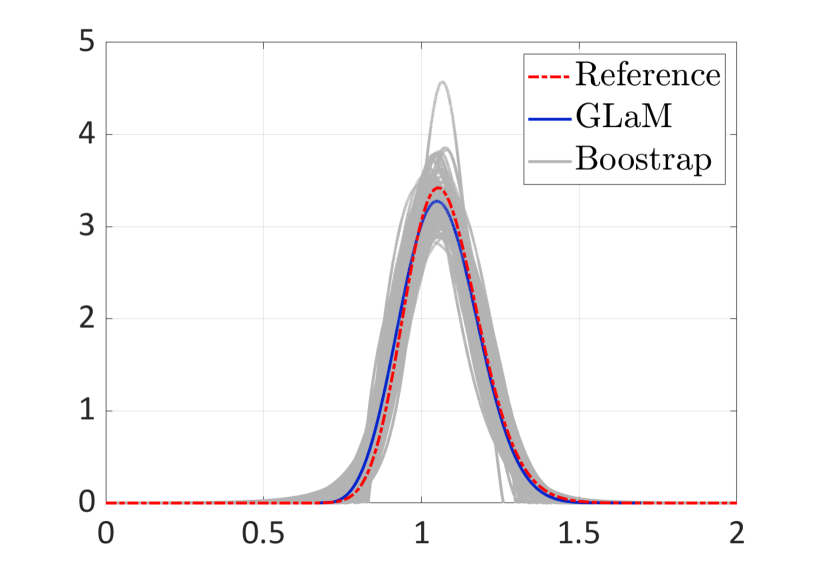
(b) PDF for $\bm{x}=(0.07,0.11)^{T}$

Figure 22: Example 1 — Uncertainty on the PDF predicted by GLaM for two values of the input parameters, using an experimental design of $N=500$. The blue line is the PDF predicted by GLaM from the 500 data points. The grey lines correspond to 100 PDFs generated by GLaM using bootstrapped experimental designs.

Possible interesting applications of the proposed method to be investigated in future studies include reliability analysis and sensitivity analysis [50]. To improve the performance of the generalized lambda surrogate model for small data sets, we plan to develop algorithms that select only important basis functions based on appropriate model selection criteria. Finally, since the generalized lambda distribution cannot represent multimodal distributions, potential extensions to mixtures of generalized lambda distributions may provide a more flexible surrogate for simulators with multimodal response distribution [51].

Appendix A Appendix

A.1 Consistency of the maximum likelihood estimator

In this section, we prove the consistency of the maximum likelihood estimator, as described in Theorem 1. For the ease of derivation, we introduce the following notation:

$$q_{\bm{c}}(\bm{x},y)=f_{Y\mid\bm{X}}\left(y\bigr{\rvert}\bm{\lambda}^{\operatorname*{PC}}(\bm{x};\bm{c})\right),\quad p_{\bm{c}}(\bm{x},y)=f_{\bm{X},Y}(\bm{x},y)=f_{X}(\bm{x})q_{\bm{c}}(\bm{x},y),$$

where $q_{\bm{c}}$ denotes the conditional PDF with model parameters $\bm{c}$, and $p_{\bm{c}}$ corresponds to the associated joint PDF. Under this setting, we assume that the true distribution $q_{0}$ belongs to the family for a particular set of coefficients $\bm{c}_{0}$, i.e., $q_{0}=q_{\bm{c}_{0}}$ and $p_{0}=p_{\bm{c}_{0}}$. We denote the probability measure of the probability space of $(\bm{X},Y)$ by $P_{0}$ and the Lebesgue measure by $\mu$.

The maximum likelihood estimation defined in Eq. 16 belongs to the generalized method of moments (GMM) [52] for which we define the loss function by

$$\ell_{\bm{c}}(\bm{x},y)=-\log\left(q_{\bm{c}}(\bm{x},y)\right)\text{1}_{q_{0}(\bm{x},y)>0}(\bm{x},y).$$ (34)

It holds that

$$\bm{c}_{0}=\arg\min_{\bm{c}}l(\bm{c}),\text{ where }l(\bm{c})={\mathbb{E}}\left[\ell_{\bm{c}}(\bm{X},Y)\right].$$

The maximum likelihood estimator is then defined by

$$\hat{\bm{c}}=\arg\min_{\bm{c}}l_{n}(\bm{c}),\text{ where }l_{n}(\bm{c})=\frac{1}{n}\sum_{i=1}^{n}\ell_{\bm{c}}\left(\bm{X}^{(i)},Y^{(i)}\right),$$

where $l_{n}$ is the empirical version of $l$.

To prove the consistency of a GMM estimator, the uniform law of large numbers is usually used. In the case of a maximum likelihood estimator for the generalized lambda model, classical methods [53] to prove the uniform law of large numbers cannot be applied directly, due to the fact that the support of $q_{\bm{c}}$ can depend on the model parameters $\bm{c}$, as shown in Eq. 4. To circumvent this problem, we use the techniques suggested by [54] for the proof.

Lemma 1.

Under the conditions described in Theorem 1, we have the following:

1. Boundedness: $\sup_{\bm{c}\in{\mathcal{C}}}q_{\bm{c}}(\bm{x},y)<+\infty$.

2. Continuity: $\forall\,\tilde{\bm{c}}\in{\mathcal{C}}$, the map $\bm{c}\mapsto q_{\bm{c}}$ is continuous at $\tilde{\bm{c}}$ for $\mu$-almost all $\left(\bm{x},y\right)\in{\mathcal{D}}_{\bm{x}}\times{\mathbb{R}}$.

Proof.

(i) As the conditions of Theorem 1 indicate that ${\mathcal{D}}_{\bm{X}}$ and ${\mathcal{C}}$ are compact, the two sets are bounded according to the Heine–Borel theorem. Hence, the value of $\bm{\lambda}^{\operatorname*{PC}}\left(\bm{x};\bm{c}\right)$ is also bounded. We denote respectively $\left\{\overline{C}_{i},i=1,\ldots,4\right\}$ and $\left\{\underline{C}_{i},i=1,\ldots,4\right\}$ as the upper and lower bounds for each component of $\bm{\lambda}$:

$$\underline{C}_{i}\leq\lambda_{i}\leq\overline{C}_{i}\quad\forall i=1,\ldots,4.$$ (35)

In addition, Eq. 15 guarantees that $\lambda_{2}^{\operatorname*{PC}}(\bm{x};\bm{c})$ is bounded away from 0, i.e., $\underline{C}_{2}>0$. Consider now Eq. 3 to evaluate the PDF of GLDs. If $u$ in Eq. 3 does not exist in $[0,1]$, $q_{\bm{c}}=0$ and thus bounded. For $u\in[0,1]$, we have

$$\frac{\lambda_{2}}{u^{\lambda_{3}-1}+(1-u)^{\lambda_{4}-1}}\leq\frac{\overline{C}_{2}}{u^{\overline{k}}+(1-u)^{\overline{k}}},$$ (36)

where

$$\overline{k}=\max\left\{\overline{C}_{3}-1,\overline{C}_{4}-1\right\}.$$

Define the function $m(u)=u^{\overline{k}}+(1-u)^{\overline{k}}$, which corresponds to the denominator of Eq. 36. For $\overline{k}=0$ and $1$, $m(u)$ is a constant function equal to $2$ and $1$, respectively. If $k\neq 0,1$, the derivative $m^{\prime}(u)=\overline{k}\left(u^{\overline{k}-1}-(1-u)^{\overline{k}-1}\right)$ is equal to $0$ only at $u=0.5$ in $[0,1]$. As a result, $\min m(u)=\min\left\{m(0),m(0.5),m(1)\right\}$. For $\overline{k}<0$, $\min m(u)=m(0.5)=2^{1-\overline{k}}$. While for $\overline{k}>0$, $\min m(u)=\min\left\{m(0),m(0.5),m(1)\right\}=\min\left\{1,2^{1-\overline{k}}\right\}$. Hence, we have $\min m(u)\geq\min\left\{1,2^{1-\overline{k}}\right\}=C_{m}$. Taking this property into account, Eq. 36 becomes

$$\frac{\lambda_{2}}{u^{\lambda_{3}-1}+(1-u)^{\lambda_{4}-1}}\leq\frac{\overline{C}_{2}}{C_{m}}=C_{q}.$$ (37)

Therefore, $\sup_{\bm{c}\in{\mathcal{C}}}q_{\bm{c}}(\bm{x},y)\leq C_{q}$.

(ii) Next, we prove the continuity. For any $\tilde{\bm{c}}\in{\mathcal{C}}$, we classify the points $(\bm{x},y)\in{\mathcal{D}}_{\bm{x}}\times{\mathbb{R}}$ into three groups based on their corresponding latent variable $\tilde{u}$: (1) $\tilde{u}\in(0,1)$, (2) $\tilde{u}$ does not exist within $[0,1]$, and (3) $\tilde{u}=0$ or $1$.

For $(\bm{x},y)$ in the first class, $y$ is an interior point of the support of the conditional distribution $q_{\tilde{\bm{c}}}(\bm{x},\cdot)$. Thereby, the following equation holds:

$$y=Q(\tilde{u};\tilde{\bm{\lambda}})=\tilde{\lambda}_{1}+\frac{1}{\tilde{\lambda}_{2}}\left(\frac{\tilde{u}^{\tilde{\lambda}_{3}}-1}{\tilde{\lambda}_{3}}-\frac{(1-\tilde{u})^{\tilde{\lambda}_{4}}-1}{\tilde{\lambda}_{4}}\right),$$ (38)

where the distribution parameters $\tilde{\bm{\lambda}}$ are obtained by evaluating $\bm{\lambda}^{\operatorname*{PC}}\left(\bm{x};\tilde{\bm{c}}\right)$. The partial derivatives of $Q(u;\bm{\lambda})$ with respect to all the relevant parameters are

$$\frac{\partial Q}{\partial u} =\frac{1}{\lambda_{2}}\left(u^{\lambda_{3}-1}+(1-u)^{\lambda_{4}-1}\right),$$ (39)

$$\frac{\partial Q}{\partial\lambda_{1}} =1,$$ (40)

$$\frac{\partial Q}{\partial\lambda_{2}} =-\frac{1}{\lambda^{2}_{2}}\left(\frac{u^{\lambda_{3}}-1}{\lambda_{3}}-\frac{(1-u)^{\lambda_{4}}-1}{\lambda_{4}}\right),$$ (41)

$$\frac{\partial Q}{\partial\lambda_{3}} =\frac{1}{\lambda_{2}\lambda^{2}_{3}}\left(u^{\lambda_{3}}\ln(u)\lambda_{3}-\left(u^{\lambda_{3}}-1\right)\right),$$ (42)

$$\frac{\partial Q}{\partial\lambda_{4}} =\frac{1}{\lambda_{2}\lambda^{2}_{4}}\left(\left((1-u)^{\lambda_{4}}-1\right)-(1-u)^{\lambda_{4}}\ln(1-u)\lambda_{4}\right).$$ (43)

It can be easily observed that Eq. 39 and Eq. 40 are continuous functions of $u\in(0,1)$ and $\bm{\lambda}$. Although Eq. 41 is undefined for $\lambda_{3}=0$ and $\lambda_{4}=0$, the limit exists according to l’Hôpital’s rule. The same holds for Eq. 42 and Eq. 43. As a result, we can extend Eqs. 41 to 43 by continuity, and thus they become continuous functions of $u\in(0,1)$ and $\bm{\lambda}$. Therefore, $Q(u,\bm{\lambda})$ is continuously differentiable. In addition, Eq. 39 is bounded away from 0. These two properties allow one to apply the implicit function theorem, and thus $u$ is a continuous function of $\bm{\lambda}$ in a neighborhood of $\tilde{\bm{\lambda}}$, which implies that $u$ is continuous at $\tilde{\bm{\lambda}}$. According to Eq. 3, the PDF is a continuous function of both $u$ and $\bm{\lambda}$. Hence, using the continuity shown before, $f_{Y}(y;\bm{\lambda})$ is continuous at $\tilde{\bm{\lambda}}$. Furthermore, $\bm{\lambda}^{\operatorname*{PC}}(\bm{x};\bm{c})$ are $C^{\infty}$ functions of $\bm{c}$, and thus $\bm{\lambda}^{\operatorname*{PC}}(\bm{x};\bm{c})$ is continuous at $\tilde{\bm{c}}$. Combining both the continuity of $f_{Y}(y;\bm{\lambda})$ and $\bm{\lambda}^{\operatorname*{PC}}(\bm{x};\bm{c})$, we have that $q_{\bm{c}}(\bm{x},y)$ is continuous at $\tilde{\bm{c}}$ for the point $(\bm{x},y)$.

Now consider a point $(\bm{x},y)$ in the second class, which implies that $y$ is outside the support of $q_{\tilde{\bm{c}}}(\bm{x},\cdot)$, say, $y$ is smaller than the lower bound of the support of $q_{\tilde{\bm{c}}}(\bm{x},\cdot)$. In this case, $q_{\tilde{\bm{c}}}(\bm{x},y)=0$. According to Eq. 4, if the lower bound is finite, it is a continuous function of $\bm{\lambda}$ and thus continuous at $\tilde{\bm{c}}$. As a result, for $\bm{c}$ within a certain neighborhood of $\tilde{\bm{c}}$, the lower bound is larger than $y$, which implies $q_{\bm{x}}(\bm{x},y)=0$ for $\bm{c}$ in this neighborhood. Thereby, $q_{\bm{c}}(\bm{x},y)$ is continuous at $\tilde{\bm{c}}$. Analogous reasoning holds for the case where $y$ is bigger than the upper bound of the support.

The last class corresponds to the case where $y$ is located on the endpoint of the support of $q_{\tilde{\bm{c}}}(\bm{x},\cdot)$. By taking $\tilde{u}=0$ and $1$ in Eq. 38 or considering directly Eq. 4, we obtain two associated deterministic functions between $\bm{x}$ and $y$. As a result, points of the third class can be represented by two curves in ${\mathcal{D}}_{x}\times{\mathbb{R}}$, whose Lebesgue measure is zero. This closes the proof of continuity. ∎

Lemma 2.

The class ${\mathcal{G}}$ defined below satisfies the uniform strong law of large numbers:

$${\mathcal{G}}=\left\{g_{\bm{c}}=\log\left(\frac{q_{\bm{c}}+q_{0}}{2q_{0}}\right)\text{1}_{q_{0}>0}:\bm{c}\in{\mathcal{C}}\right\}.$$ (44)

Proof.

According to the continuity property in Lemma 1, it is obvious that for all $\tilde{\bm{c}}\in{\mathcal{C}}$, the map $\bm{c}\mapsto g_{\bm{c}}$ is continuous at $\tilde{\bm{c}}$ for $\mu$-almost all $(\bm{x},y)\in{\mathcal{D}}\times{\mathbb{R}}$. By assumption, the probability measure $P_{0}$ is absolutely continuous with respect to $\mu$, and thus $g_{\bm{c}}$ is continuous for $P_{0}$-almost all $(\bm{x},y)\in{\mathcal{D}}\times{\mathbb{R}}$.

Define $G$ as the envelope function of the class ${\mathcal{G}}$, i.e., $G(\bm{x},y)=\sup_{\bm{c}\in{\mathcal{C}}}\left\lvert g_{\bm{c}}(\bm{x},y)\right\rvert$. Let us prove that $G\in L_{1}(P_{0})$, where $L_{1}(P_{0})$ denotes the set of absolutely integrable functions with respect to $P_{0}$.

Taking the boundedness property in Lemma 1 into account, we obtain

$$g_{\bm{c}}(\bm{x},y)\leq\log\left(\frac{2C_{q}}{q_{0}(\bm{x},y)}\right)=\log(2C_{q})-\log(q_{0}(\bm{x},y)).$$ (45)

Obviously, $g_{\bm{c}}(\bm{x},y)\geq-\log(2)$. Therefore,

$$\begin{split}\left\lvert g_{\bm{c}}(\bm{x},y)\right\rvert&\leq\max\left\{\log(2),\left\lvert\log(2C_{q})\right\rvert+\left\lvert\log(q_{0}(\bm{x},y))\right\rvert\right\}\\ &\leq\log(2)+\left\lvert\log(C_{q})\right\rvert+\left\lvert\log(q_{0}(\bm{x},y))\right\rvert.\end{split}$$ (46)

Because the inequality is independent of $\bm{c}$, we have

$$\begin{split}G(\bm{x},y)&\leq\log(2)+\left\lvert\log(C_{q})\right\rvert+\left\lvert\log(q_{0}(\bm{x},y))\right\rvert,\\ {\mathbb{E}}\left[G(\bm{X},Y)\right]&\leq\log(2)+\left\lvert\log(C_{q})\right\rvert+{\mathbb{E}}\left[\left\lvert\log(q_{0}(\bm{X},Y)\right\rvert\right].\end{split}$$ (47)

Now consider the last term in Eq. 47:

$$\begin{split}{\mathbb{E}}\left[\left\lvert\log(q_{0}(\bm{X},Y)\right\rvert\right]&=\int_{{\mathcal{D}}_{\bm{x}}\times{\mathbb{R}}}\left\lvert\log\left(q_{0}(\bm{x},y)\right)\right\rvert p_{0}(\bm{x},y)\mathrm{d}\bm{x}\mathrm{d}y\\ &=\int_{{\mathcal{D}}_{\bm{x}}}\left(\int_{{\mathbb{R}}}\left\lvert\log\left(q_{0}(\bm{x},y)\right)\right\rvert q_{0}(\bm{x},y)\mathrm{d}y\right)f_{\bm{X}}(\bm{x})\mathrm{d}\bm{x}.\end{split}$$ (48)

Through a change of variables, the integral within the parenthesis of Eq. 48 can be calculated as

$$B(\bm{x})=\int_{{\mathbb{R}}}\left\lvert\log\left(q_{0}(\bm{x},y)\right)\right\rvert q_{0}(\bm{x},y)\mathrm{d}y=\int_{0}^{1}\left\lvert\log\left(\frac{\lambda_{2}}{u^{\lambda_{3}-1}+(1-u)^{\lambda_{4}-1}}\right)\right\rvert\mathrm{d}u,$$ (49)

where $\bm{\lambda}=\bm{\lambda}^{\operatorname*{PC}}(\bm{x};\bm{c}_{0})$. According to Eq. 35, we have

$$\begin{split}B(\bm{x})&\leq\int_{0}^{1}\left\lvert\log(\lambda_{2})\right\rvert+\left\lvert\log\left(u^{\lambda_{3}-1}+(1-u)^{\lambda_{4}-1}\right)\right\rvert\mathrm{d}u\\ &\leq k_{2}+\int_{0}^{1}\max\left\{\left\lvert\log\left(u^{\underline{k}}+(1-u)^{\underline{k}}\right)\right\rvert,\left\lvert\log\left(u^{\overline{k}}+(1-u)^{\overline{k}}\right)\right\rvert\right\}\mathrm{d}u,\end{split}$$ (50)

where

$$k_{2}=\max\left\{\left\lvert\log\left(\overline{C}_{2}\right)\right\rvert,\left\lvert\log\left(\underline{C}_{2}\right)\right\rvert\right\},\;\underline{k}=\min\left\{\underline{C}_{3}-1,\underline{C}_{4}-1\right\},\;\overline{k}=\max\left\{\overline{C}_{3}-1,\overline{C}_{4}-1\right\}.$$

Using the symmetry of the integrand, we get

$$\begin{split}B(\bm{x})&\leq k_{2}+2\cdot\max\left\{\int_{0}^{\frac{1}{2}}\left\lvert\log\left(u^{\underline{k}}+(1-u)^{\underline{k}}\right)\right\rvert\mathrm{d}u,\int_{0}^{\frac{1}{2}}\left\lvert\log\left(u^{\overline{k}}+(1-u)^{\overline{k}}\right)\right\rvert\mathrm{d}u\right\}\\ &\leq k_{2}+2\cdot\left(\int_{0}^{\frac{1}{2}}\left\lvert\log\left(u^{\underline{k}}+(1-u)^{\underline{k}}\right)\right\rvert\mathrm{d}u+\int_{0}^{\frac{1}{2}}\left\lvert\log\left(u^{\overline{k}}+(1-u)^{\overline{k}}\right)\right\rvert\mathrm{d}u\right).\end{split}$$ (51)

Without loss of generality, we now study the property of the integral

$$\int_{0}^{\frac{1}{2}}\left\lvert\log\left(u^{k}+(1-u)^{k}\right)\right\rvert\mathrm{d}u.$$ (52)

For $k=0$, Eq. 52 is equal to $\frac{1}{2}\log(2)$. For $k>0$, we have $u^{k}\leq(1-u)^{k}$, and thus

$$\begin{split}\int_{0}^{\frac{1}{2}}\left\lvert\log\left(u^{k}+(1-u)^{k}\right)\right\rvert\mathrm{d}u\leq\int_{0}^{\frac{1}{2}}\left\lvert\log\left(2(1-u)^{k}\right)\right\rvert\mathrm{d}u&\leq\frac{1}{2}\log(2)-\int_{0}^{\frac{1}{2}}k\log(1-u)\mathrm{d}u\\ &=\frac{1}{2}\log(2)+\frac{k}{2}\left(1-\log(2)\right).\end{split}$$ (53)

Through similar calculation, for $k<0$, we have

$$\begin{split}\int_{0}^{\frac{1}{2}}\left\lvert\log\left(u^{k}+(1-u)^{k}\right)\right\rvert\mathrm{d}u\leq\int_{0}^{\frac{1}{2}}\left\lvert\log\left(2u^{k}\right)\right\rvert\mathrm{d}u&\leq\frac{1}{2}\log(2)+\int_{0}^{\frac{1}{2}}k\log(u)\mathrm{d}u\\ &=\frac{1}{2}\log(2)+\frac{-k}{2}\left(\log(2)+1\right).\end{split}$$ (54)

As a result, Eq. 52 is finite. More precisely,

$$\int_{0}^{\frac{1}{2}}\left\lvert\log\left(u^{k}+(1-u)^{k}\right)\right\rvert\mathrm{d}u\leq\frac{1}{2}\log(2)+\frac{\left\lvert k\right\rvert}{2}\left(\log(2)+1\right).$$ (55)

Equation 55 implies

$$B(\bm{x})\leq k_{2}+\log(2)+\left(\left\lvert\underline{k}\right\rvert+\left\lvert\overline{k}\right\rvert\right)\left(\log(2)+1\right)=C_{B}.$$ (56)

By inserting Eq. 56 into Eq. 48, we obtain

$${\mathbb{E}}\left[\left\lvert\log(q_{0}(\bm{X},Y)\right\rvert\right]\leq C_{B}.$$ (57)

Then, according to Eq. 47, the envelope function $G$ fulfills

$$\begin{split}{\mathbb{E}}\left[G(\bm{X},Y)\right]&\leq\log(2)+\left\lvert\log(C_{q})\right\rvert+{\mathbb{E}}\left[\left\lvert\log\left(q_{0}(\bm{X},Y)\right)\right\rvert\right]\\ &=\log(2)+\left\lvert\log(C_{q})\right\rvert+C_{B}<+\infty.\end{split}$$ (58)

Since $G$ is always positive according to its definition, Eq. 58 means $G\in L_{1}(P_{0})$. The continuity and the property of the envelope function $G$ shown above allow applying [54, Lemma 3.10], which guarantees that ${\mathcal{G}}$ satisfies the uniform weak law of large numbers:

$$\sup_{\bm{c}\in{\mathcal{C}}}\left(\frac{1}{n}\sum_{i=1}^{n}g_{\bm{c}}\left(\bm{X}^{(i)},Y^{(i)}\right)-{\mathbb{E}}\left[g_{\bm{c}}\left(\bm{X},Y\right)\right]\right)\xrightarrow[n\rightarrow+\infty]{P}0.$$ (59)

Finally, [55, Theorem 22] extends the convergence to almost surely, which is the uniform strong law of large numbers. ∎

Now, we have all the ingredients to prove Theorem 1.

Proof.

Following [54, Lemma 4.1, 4.2], it can be easily shown that

$$0\leq\int_{{\mathcal{D}}_{\bm{x}}}h^{2}\left(q_{\hat{\bm{c}}},q_{0}\mid\bm{x}\right)f_{\bm{X}}(\bm{x})\mathrm{d}\bm{x}\leq 8\left(\sum_{i=1}^{N}g_{\hat{\bm{c}}}\left(\bm{X}^{(i)},Y^{(i)}\right)-{\mathbb{E}}\left[g_{\hat{\bm{c}}}\left(\bm{X},Y\right)\right]\right),$$ (60)

where the Hellinger distance is given by

$$h^{2}\left(q_{\hat{\bm{c}}},q_{0}\mid\bm{x}\right)=\frac{1}{2}\int_{{\mathbb{R}}}\left(\sqrt{q_{\hat{\bm{c}}}(\bm{x},y)}-\sqrt{q_{0}(\bm{x},y)}\right)^{2}\mathrm{d}y.$$

According to Lemma 2, Eq. 60 implies

$$\int_{{\mathcal{D}}_{\bm{x}}}h^{2}\left(q_{\hat{\bm{c}}},q_{0}\mid\bm{x}\right)f_{\bm{X}}(\bm{x})\mathrm{d}\bm{x}\xrightarrow{\text{a.s.}}0,$$ (61)

which is called the Hellinger consistency.

We define the function

$$R(\bm{c})=\int_{{\mathcal{D}}_{\bm{x}}}h^{2}\left(q_{\bm{c}},q_{0}\mid\bm{x}\right)f_{\bm{X}}(\bm{x})\mathrm{d}\bm{x}.$$ (62)

According to Lemma 1, $\forall\tilde{\bm{c}}\in{\mathcal{C}}$, the map $\bm{c}\mapsto\left(\sqrt{q_{\bm{c}}}-\sqrt{q_{0}}\right)^{2}$ is continuous at $\tilde{\bm{c}}$ for all $\bm{x}\in{\mathcal{D}}_{x}$ and almost all $y\in{\mathbb{R}}$. Since $\left(\sqrt{q_{\bm{c}}}-\sqrt{q_{0}}\right)^{2}\leq q_{\bm{c}}+q_{0}$, and $\int_{{\mathbb{R}}}\left(q_{\bm{c}}+q_{0}\right)\mathrm{d}y=2<+\infty$, the map $\bm{c}\mapsto h^{2}\left(q_{\bm{c}},q_{0}\mid\bm{x}\right)$ is continuous for all $\bm{x}\in{\mathcal{D}}_{\bm{x}}$, which is guaranteed by the generalized Lebesgue dominated convergence theorem. Similarly, the map $\bm{c}\mapsto R(\bm{c})$ is also continuous.

Without going into lengthy discussions, it can be shown that the GLD is not identifiable only for $\lambda_{3}=\lambda_{4}=1$ and $\lambda_{3}=\lambda_{4}=2$. In other words, by excluding two points in the $\lambda_{3}-\lambda_{4}$ plane, different values of $\bm{\lambda}$ lead to different distributions. Note that the two exceptions are the only two cases where the corresponding distributions are uniform distributions. As a result, the last condition in Theorem 1 excludes the nonidentifiable cases. Furthermore, $\bm{\lambda}^{\operatorname*{PC}}(\bm{x};\bm{c})$ are polynomials in $\bm{x}$ and linear in $\bm{c}$. Therefore, for $\bm{c}\neq\tilde{\bm{c}}$, $\bm{\lambda}^{\operatorname*{PC}}(\bm{x};\bm{c})$ and $\bm{\lambda}^{\operatorname*{PC}}\left(\bm{x};\tilde{\bm{c}}\right)$ are not identical for $\mu$-almost all $\bm{x}\in{\mathbb{R}}^{M}$, and thus for $P_{\bm{X}}$-almost all $\bm{x}\in{\mathcal{D}}_{\bm{X}}$. Hence, there exists a set $\Omega_{\bm{x}}$ with $P_{\bm{X}}(\Omega_{\bm{x}})>0$ such that as long as $\bm{c}\neq\bm{c}_{0}$, $h\left(q_{\bm{c}},q_{0}\mid\bm{x}\right)>0$ $\forall\bm{x}\in\Omega_{\bm{x}}$, which implies the uniqueness. Finally, combining Eq. 61 with the continuity and uniqueness of $R(\bm{c})$, we have $\hat{\bm{c}}\xrightarrow{\text{a.s.}}\bm{c}_{0}$. ∎

References

- [1] I. Abdallah, C. Lataniotis, and B. Sudret. Parametric hierarchical Kriging for multi-fidelity aero-servo-elastic simulators—application to extreme loads on wind turbines. Prob. Engrg. Mech., 55:67–77, 2019.
- [2] S. Shreve. Stochastic Calculus for Finance II. Springer, New York, 2004.
- [3] T. Britton. Stochastic epidemic models: A survey. Math. Biosci., 225:24–35, 2010.
- [4] M.N. Jimenez, O.P. Le Maître, and O.M. Knio. Nonintrusive polynomial chaos expansions for sensitivity analysis in stochastic differential equations. SIAM/ASA J. Uncertain. Quantif., 5:378–402, 2017.
- [5] S. Azzi, Y. Huang, B. Sudret, and J. Wiart. Surrogate modeling of stochastic functions—application to computational electromagnetic dosimetry. Int. J. Uncertain. Quantif., 9:351–363, 2019.
- [6] C.E. Rasmussen and C.K.I. Williams. Gaussian Processes for Machine Learning. Adapt. Comput. Mach. Learn. MIT Press, Cambridge, Massachusetts, Internet edition, 2006.
- [7] G. Blatman and B. Sudret. Adaptive sparse polynomial chaos expansion based on Least Angle Regression. J. Comput. Phys., 230:2345–2367, 2011.
- [8] V. Moutoussamy, S. Nanty, and B. Pauwels. Emulators for stochastic simulation codes. ESAIM Math. Model. Numer. Anal., 48:116–155, 2015.
- [9] T. Browne, B. Iooss, L. Le Gratiet, J. Lonchampt, and E. Rémy. Stochastic simulators based optimization by Gaussian process metamodels—application to maintenance investments planning issues. Quality Reliab. Eng. Int., 32(6):2067–2080, 2016.
- [10] X. Zhu and B. Sudret. Replication-based emulation of the response distribution of stochastic simulators using generalized lambda distributions. Int. J. Uncertain. Quantif., 10:249–275, 2020.
- [11] P. McCullagh and J. Nelder. Generalized Linear Models, volume 37 of Monogr. Statist. Appl. Probab. Chapman and Hall/CRC, 2nd edition, 1989.
- [12] T. Hastie and R. Tibshirani. Generalized Additive Models, volume 43 of Monogr. on Statist. Appl. Probab. Chapman and Hall, 1990.
- [13] J. Fan and I. Gijbels. Local Polynomial Modelling and Its Applications. Monogr. on Statist. Appl. Probab. 66. Chapman and Hall, 1996.
- [14] P. Hall, J. Racine, and Q. Li. Cross-validation and the estimation of conditional probability densities. J. Amer. Statist. Assoc., 99:1015–1026, 2004.
- [15] S. Efromovich. Dimension reduction and adaptation in conditional density estimation. J. Amer. Statist. Assoc., 105:761–774, 2010.
- [16] A.B. Tsybakov. Introduction to Nonparametric Estimation. Springer Ser. Statist. Springer, Cambridge, New York, 2009.
- [17] M. Freimer, G. Kollia, G.S. Mudholkar, and C.T. Lin. A study of the generalized Tukey lambda family. Comm. Statist. Theory Methods, 17:3547–3567, 1988.
- [18] Z.A. Karian and E.J. Dudewicz. Fitting Statistical Distributions: The Generalized Lambda Distribution and Generalized Bootstrap Methods. CRC Press, 2000.
- [19] O.G. Ernst, A. Mugler, H.J. Starkloff, and E. Ullmann. On the convergence of generalized polynomial chaos expansions. ESAIM Math. Model. Numer. Anal., 46:317–339, 2012.
- [20] C. Soize and R. Ghanem. Physical systems with random uncertainties: Chaos representations with arbitrary probability measure. SIAM J. Sci. Comput., 26(2):395–410, 2004.
- [21] D. Xiu and G.E. Karniadakis. The Wiener–Askey polynomial chaos for stochastic differential equations. SIAM J. Sci. Comput., 24(2):619–644, 2002.
- [22] W. Gautschi. Orthogonal Polynomials: Computation and Approximation. Oxford University Press, 2004.
- [23] G. Blatman and B. Sudret. An adaptive algorithm to build up sparse polynomial chaos expansions for stochastic finite element analysis. Prob. Engrg. Mech., 25:183–197, 2010.
- [24] E. Torre, S. Marelli, P. Embrechts, and B. Sudret. Data-driven polynomial chaos expansion for machine learning regression. J. Comput. Phys., 388:601–623, 2019.
- [25] J.D. Jakeman, F. Franzelin, A. Natayan, M. Eldred, and D. Plfüger. Polynomial chaos expansions for dependent random variables. Comput. Methods Appl. Mech. Engrg., 351:643–666, 2019.
- [26] T. Steihaug. The conjugate gradient method and trust regions in large scale optimization. SIAM J. Numer. Anal., 20(3):626–637, 1983.
- [27] D.V. Arnold and N. Hansen. A (1+1)-CMA-ES for constrained optimisation. In Terence Soule and Jason H. Moore, editors, Proceedings of the Genetic and Evolutionary Computation Conference 2012 (GECCO 2012) (Philadelphia, PA), pages 297–304, 2012.
- [28] M. Moustapha, C. Lataniotis, P. Wiederkehr, P.-R. Wagner, D. Wicaksono, S. Marelli, and B. Sudret. UQLib User Manual. Technical report, Chair of Risk, Safety and Uncertainty Quantification, ETH Zurich, Switzerland, 2019. Report # UQLab-V1.3-201.
- [29] A.C. Harvey. Estimating regression models with multiplicative heteroscedasticity. Econometrica, 44:461–465, 1976.
- [30] W.A. Sadler and M.H. Smith. Estimation of the response error relationship in immunoassay. Clinical Chem., 31:1802–1805, 1985.
- [31] B. Ankenman, B. Nelson, and J. Staum. Stochastic Kriging for simulation metamodeling. Oper. Res., 58:371–382, 2009.
- [32] J.P. Murcia, P.E. Réthoré, N. Dimitrov, A. Natarajan, J. D. Sørensen, P. Graf, and T. Kim. Uncertainty propagation through an aeroelastic wind turbine model using polynomial surrogates. Renewable Energy, 119:910–922, 2018.
- [33] J.A. Nelder and D. Pregibon. An extended quasi-likelihood function. Biometrika, 74:221–232, 1987.
- [34] M. Davidian and R.J. Carroll. Variance function estimation. J. Amer. Statist. Assoc., 82:1079–1091, 1987.
- [35] P.W. Goldberg, C.K.I. Williams, and C. M. Bishop. Regression with input-dependent noise: A Gaussian process treatment. In Proceedings of the 10th International Conference on Advances in Neural Information Processing Systems (NIPS10), Colorado, USA, pages 493–499, 1997.
- [36] A. Marrel, B. Iooss, S. Da Veiga, and M. Ribatet. Global sensitivity analysis of stochastic computer models with joint metamodels. Stat. Comput., 22:833–847, 2012.
- [37] J.M. Wooldridge. Introductory Econometrics: A Modern Approach. Cengage Learning, 5th edition, 2013.
- [38] S. Marelli and B. Sudret. UQLab User Manual—Polynomial Chaos Expansions. Technical report, Chair of Risk, Safety and Uncertainty Quantification, ETH Zurich, Switzerland, 2019. Report # UQLab-V1.3-104.
- [39] T. Hayfield and J.S. Racine. Nonparametric econometrics: The np package. J. Statist. Software, 2008.
- [40] M. Binois, J. Huang, R.B. Gramacy, and M. Ludkovski. Replication or exploration? Sequential design for stochastic simulation experiments. J. Comput. Graph. Statist., 61:7–23, 2019.
- [41] M. Binois, R.B. Gramacy, and M. Ludkovski. Practical heteroscedastic Gaussian process modeling for large simulation experiments. J. Comput. Graph. Statist., 27:808–821, 2018.
- [42] M.D. McKay, R.J. Beckman, and W.J. Conover. A comparison of three methods for selecting values of input variables in the analysis of output from a computer code. Technometrics, 21(2):239–245, 1979.
- [43] C. Villani. Optimal Transport, Old and New. Springer, Berlin, 2009.
- [44] A.J. McNeil, R. Frey, and P. Embrechts. Quantitative Risk Management: Concepts, Techniques, and Tools. Princeton Series in Finance. Princeton University Press, Princeton, NJ, 2005.
- [45] K. Reddy and V. Clinton. Simulating stock prices using geometric Brownian motion: Evidence from Australian companies. Australasian Accounting, Business Finance J., 10(3):23–47, 2016.
- [46] A.G.Z. Kemna and A.C.F. Vorst. A pricing method for options based on average asset values. J. Bank. Finance, 14:113–129, 1990.
- [47] D.T. Gillespie. Exact stochastic simulation of coupled chemical reactions. J. Phys. Chem., 81:2340–2361, 1977.
- [48] D. Merl, L.R. Johnson, R.B. Gramacy, and M. Mangel. A statistical framework for the adaptive management of epidemiological interventions. PLoS ONE, 4:e5089, 2009.
- [49] B. Efron. The jackknife, the bootstrap and other resampling plans, volume 38. SIAM, 1982.
- [50] X. Zhu and B. Sudret. Global sensitivity analysis for stochastic simulators based on generalized lambda surrogate models. Reliab. Engrg. Syst. Safety, 214(107815), 2021.
- [51] A. Fadikar, D. Higdon, J. Chen, B. Lewis, S. Venkatramanan, and M. Marathe. Calibrating a stochastic, agent-based model using quantile-based emulation. SIAM/ASA J. Uncertain. Quantif., 6(4):1685–1706, 2018.
- [52] L.P. Hansen. Large sample properties of generalized method of moments estimators. Econometrica, 50:1029–1054, 1982.
- [53] W.K. Newey and D. McFadden. Large sample estimation and hypothesis testing, chapter 36, pages 2111–2245. Elsevier, 1994.
- [54] S. van de Geer. Empirical Processes in M-Estimation. Cambridge Series in Statistical and Probabilistic Mathematics. Cambridge University Press, Cambridge, 2000.
- [55] M. Talagrand. The Glivenko-Cantelli problem. Ann. Probab., 15:837–870, 1987.