Abstract

The 2+1+1 decomposition of space-time is useful in monitoring the temporal evolution of gravitational perturbations/waves in space-times with a spatial direction singled-out by symmetries. Such an approach based on a perpendicular double foliation has been employed in the framework of dark matter and dark energy motivated scalar-tensor gravitational theories for the discussion of the odd sector perturbations of spherically symmetric gravity. For the even sector however the perpendicularity has to be suppressed in order to allow for suitable gauge freedom, recovering the 10th metric variable. The 2+1+1 decomposition of the Einstein-Hilbert action leads to the identification of the canonical pairs, the Hamiltonian and momentum constraints. Hamiltonian dynamics is then derived via Poisson brackets.

x 10.3390/—— xx Academic Editor: name Received: date; Accepted: date; Published: date Hamiltonian dynamics of doubly-foliable space-times Cecília Gergely¹, Zoltán Keresztes² and László Árpád Gergely^3,* Cecília Gergely, Zoltán Keresztes and László Árpád Gergely Correspondence: laszlo.a.gergely@gmail.com; Tel.: +36702020800

1 Introduction

In the curved space-time of general relativity gravitational waves propagate with the speed of light (the velocity limit), correcting the Newtonian description of gravity. Whenever a reference system is chosen, time needs to be singled out. In the 3+1 decomposition of space-time, known as the Arnowitt-Deser-Misner (ADM) formalism of gravity ADM , the constant time 3-surfaces form a foliation. While the time parameter is constant on each hypersurface, it changes monotonically from one hypersurface to the other. The role of the 4-dimensional metric $\widetilde{g}_{ab}$ (with$\ 10$ independent components) is taken by the metric induced on the 3-dimensional hypersurfaces ($6$ variables) and their extrinsic curvature ($6$ variables), which generate canonical pairs. Einstein equations are replaced by the Hamiltonian evolution of these canonical pairs. Beside these there are constraint equations to be fulfilled in each instant (on each hypersurface). These are the Hamiltonian and Diffeomorphism constraints. In the generic case of the 3+1 decompositions there is no preferred time, the formalism has to be valid for any possible temporal choices ("many-fingered time" formalism manyfingeredtime ; manyfingeredtime2 ). Preferred choices arise by either imposing coordinate conditions K-coord1 ; K-coord2 or by filling space-time with an adequate reference fluid K-ref1 ; K-ref2 . Although the 3+1 decomposition breaks space-time covariance, a manifestly covariant canonical formalism based on the hyperspace (defined by all space-like hypersurfaces) has been also proposed K_hyp1 ; K_hyp2 ; K_hyp3 ; K_hyp4 . The ADM decomposition has been generalised for some of the modified gravity theories as well, e.g. for the $f(R)$ gravitational theories Mongwane .

If in addition a spatial direction plays a special role, the 2+1+1 decomposition of space-time may prove useful. This special role can be provided by a Killing-symmetry, for example the radial directions in either spherical or cylindrical symmetric space-times are such singled-out directions. We do not explore however simplifications arising from the imposition of symmetries, as for example applying mini-superspace or midi-superspace approaches K_cyl ; K_SCHW . The scenario we have in mind is to discuss generic perturbations of a background with certain symmetry. In the most generic case both singled-out directions have expansion, shear and vorticity Clarkson . The corresponding optical scalars were explored in the discussion of perturbations of spherically symmetric space-times CB , also for the discussion of gravitational waves in anisotropic Kantowski-Sachs space-times KFBDG .

In another, much simpler 2+1+1 decomposition formalism the decomposition is made along a perpendicular double foliation s+1+1a ; s+1+1b . This formalism has been employed in the framework of dark matter and dark energy motivated scalar-tensor gravitational theories in the discussion of the odd sector perturbations of spherically symmetric gravity in the effective field theory approach KGT . The requirement of perpendicularity however consumes one gauge degree of freedom by fixing a metric function to vanish. This has posed no problem in the discussion of the odd sector, however for the even sector it generates an arbitrary function in the solution, hampering the physical interpretation of perturbations. Therefore a modified 2+1+1 decomposition formalism would be desireble, which keeps the relative simplicity of the formalism of s+1+1a ; s+1+1b (as compared to the formalism exploring optical scalars Clarkson ), but employs $10$ metric functions instead of$\ 9$, hence becomes suitable for the discussion of the even sector. Such a formalism could be worked out at the price of relaxing the perpendicularity requirement 2+1+1paper .

In this conference report we summarise the main feature of this new formalism and sketch the derivation of the Hamiltonian formalism, without insisting on the involved computational details and related proofs of the statements, which are given in Ref. 2+1+1paper together with additional details.

Latin indices denote 4-dimensional space-time indices. Boldface lowercase (as $\mathbf{i}$) or uppercase (as $\mathbf{A}$) latin letters count 2-dimensional or 4-dimensional basis vectors.

2 The nonorthogonal double foliation

We generalise the orthogonal 2+1+1 decomposition of Refs. s+1+1a ; s+1+1b such that the hypersurfaces $\mathcal{S}_{t}$ of constant $t$ and $\mathfrak{M}_{\chi}$ of constant $\chi$ with normal vectors $n^{a}$ and $l^{a}$, respectively, are nonorthogonal, as presented on Fig. 1.

Their intersection is the surface $\Sigma_{t\chi}$, with an adapted vector basis $\left\{F_{\mathbf{i}}\right\}$. We introduce two orthonormal bases adapted to the two foliations, as follows: $f_{\mathbf{A}}=\left\{n,m,F_{\mathbf{i}}\right\}$ and $g_{\mathbf{A}}=\left\{k,l,F_{\mathbf{i}}\right\}$. The 4-dimensional metric can then be decomposed in both:

$$\tilde{g}_{ab} = -n_{a}n_{b}+m_{a}m_{b}+g_{ab}~{},$$ (1)

$$\tilde{g}_{ab} = -k_{a}k_{b}+l_{a}l_{b}+g_{ab}~{}.$$ (2)

Here $g_{ab}$ is the metric induced on $\Sigma_{t\chi}$.

The temporal and selected spatial evolution vectors in the $f_{\mathbf{A}}$ basis are:

$$\left(\frac{\partial}{\partial t}\right)^{a} = Nn^{a}+N^{a}+\mathcal{N}m^{a}~{},$$ (3)

$$\left(\frac{\partial}{\partial\chi}\right)^{a} = Mm^{a}+M^{a}+\mathcal{M}n^{a}~{}.$$ (4)

They define a coordinate-basis, the duality relations of which imply 2+1+1paper

$$\mathcal{M}=0~{},$$ (5)

making manifest that $\partial/\partial\chi$ is tangent to $\mathcal{S}_{t}$. The shift component $\mathcal{N}$ arises due to the nonorthogonality of the foliations and generates all new terms arising as compared to the formalism presented in Refs. s+1+1a ; s+1+1b , where $\mathcal{N}=0$ was imposed. With the introduction of a nonvanishing $\mathcal{N}$ full gauge freedom is reestablished, with $10$ metric components in the formalism ($3$ for $g_{ab}$, $2$ for $M^{a}$ and $N^{a}$ each, one for each of the lapses $N$, $M$ and shift component $\mathcal{N}$). At times it will be convenient to parametrize this $10^{th}$ metric function as $\mathcal{N}=N\tanh\phi$ and also employ the notations $\mathfrak{s}=\sinh\phi$, $\mathfrak{c}=\cosh\phi$. This is especially convenient in proving 2+1+1paper that the two bases are related by a Lorentz-rotation:

$$\left({\begin{array}[]{c}k^{a}\\ l^{a}\\ \end{array}}\right)=\left({\begin{array}[]{cc}\mathfrak{c}&\mathfrak{s}\\ \mathfrak{s}&\mathfrak{c}\\ \end{array}}\right)\left({\begin{array}[]{c}n^{a}\\ m^{a}\\ \end{array}}\right)$$ (6)

also to derive the decomposition of the evolution vectors in the basis $g_{\mathbf{A}}$:

$$\left(\frac{\partial}{\partial t}\right)^{a} = \frac{N}{\mathfrak{c}}k^{a}+N^{a}~{},$$ (7)

$$\left(\frac{\partial}{\partial\chi}\right)^{a} = M\left(-\mathfrak{s}k^{a}+\mathfrak{c}l^{a}\right)+M^{a}~{}.$$ (8)

Note that $\partial/\partial t$ is manifestly tangent to the hypersurface $\mathfrak{M}_{\chi}$.

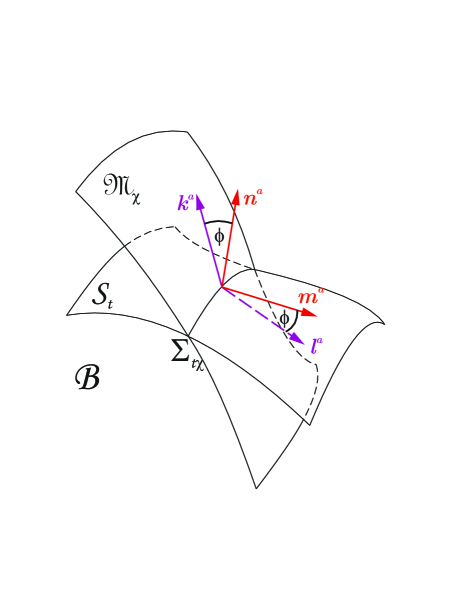
Figure 1: The hypersurfaces of the nonorthogonal double foliation and the adapted bases.

Finally, in the basis $f_{\mathbf{A}}$ it is straightforward to check

$$\left[m,F_{\mathbf{j}}\right]^{a}n_{a}=0~{},$$ (9)

reassuring (due to the Frobenius Theorem) that $n^{a}$ is hypersurface-orthogonal and

$$\left[n,F_{\mathbf{j}}\right]^{a}m_{a}=\frac{M}{N}\partial_{\mathbf{j}}\left(\frac{\mathcal{N}}{M}\right)~{},$$ (10)

implying that the vector $m^{a}$ has vorticity. Similarly, in the basis $g_{\mathbf{A}}$ we find that $l^{a}$ is hypersurface-orthogonal and $k^{a}$ has vorticity:

$$\left[k,F_{\mathbf{j}}\right]^{a}l_{a} = 0~{},$$ (11)

$$\left[l,F_{\mathbf{j}}\right]^{a}k_{a} = \frac{N}{\mathfrak{c}^{2}M}\partial_{\mathbf{j}}\left(\frac{\mathfrak{sc}M}{N}\right)~{}.$$ (12)

Hence the $10^{th}$ metric function $\mathcal{N}$ bears a double interpretation: (1) it gives the angle of the Lorentz-rotation between the two bases, and (2) generates the vorticity of the complementary basis vectors $m^{a}$ and $k^{a}$. More details of these interpretations will be presented in Ref. 2+1+1paper .

3 The 2+1+1 decomposition of covariant derivatives

The projected covariant derivative of any tensor $T_{b_{1}...b_{r}}^{a_{1}...a_{r}}$ defined on $\Sigma_{t\chi}$ arises by projecting in all indices with $g_{a}^{b}$:

$$D_{a}T_{b_{1}...b_{q}}^{a_{1}...a_{r}}\equiv g_{a}^{c}g_{c_{1}}^{a_{1}}...g_{c_{r}}^{a_{r}}g_{b_{1}}^{d_{1}}...g_{b_{q}}^{d_{q}}\tilde{\nabla}_{c}T_{d_{1}...d_{q}}^{c_{1}...c_{r}}~{}.$$ (13)

The $D$-derivative obtained in this way is related to the connection compatible with the 2-metric due to the property

$$D_{a}g_{bc}=0~{}.$$ (14)

It will be of particular importance to 2+1+1 decompose the covariant derivatives of the basis vectors. We found:

$$\tilde{\nabla}_{a}n_{b}=K_{ab}+2m_{(a}\mathcal{K}_{b)}+m_{a}m_{b}\mathcal{K}-n_{a}\left(\mathfrak{a}_{b}-m_{b}\mathcal{L}^{\ast}\right)~{},$$ (15)

$$\tilde{\nabla}_{a}m_{b}=L_{ab}^{\ast}+n_{a}\mathcal{L}_{b}^{\ast}+n_{b}\mathcal{K}_{a}+n_{a}n_{b}\mathcal{L}^{\ast}+m_{a}\left(\mathfrak{b}_{b}^{\ast}+n_{b}\mathcal{K}\right)~{},$$ (16)

$$\tilde{\nabla}_{a}k_{b}=K_{ab}^{\ast}+l_{a}\mathcal{K}_{b}^{\ast}+l_{b}\mathcal{L}_{a}+l_{a}l_{b}\mathcal{K}^{\ast}-k_{a}\left(\mathfrak{a}_{b}^{\ast}-l_{b}\mathcal{L}\right)~{},$$ (17)

$$\tilde{\nabla}_{a}l_{b}=L_{ab}+2k_{(a}\mathcal{L}_{b)}+k_{a}k_{b}\mathcal{L}+l_{a}\left(\mathfrak{b}_{b}+k_{b}\mathcal{K}^{\ast}\right)~{},$$ (18)

where $K_{ab}=g_{a}^{c}g_{b}^{d}\tilde{\nabla}_{c}n_{d}$, $L_{ab}^{\ast}=g_{a}^{c}g_{b}^{d}\tilde{\nabla}_{c}m_{d}$, $K_{ab}^{\ast}=g_{a}^{c}g_{b}^{d}\tilde{\nabla}_{c}k_{d}$ and $L_{ab}=g_{a}^{c}g_{b}^{d}\tilde{\nabla}_{c}l_{d}$ are extrinsic curvatures of the surface $\Sigma_{t\chi}$; $\mathcal{K}_{a}=g_{a}^{c}m^{d}\tilde{\nabla}_{c}n_{d}$ and $\mathcal{L}_{a}=-g_{a}^{c}k^{d}\tilde{\nabla}_{c}l_{d}$ are normal fundamental forms; $\mathcal{K}=m^{d}m^{c}\tilde{\nabla}_{c}n_{d}$, $\mathcal{L}^{\ast}=n^{c}n^{d}\tilde{\nabla}_{c}m_{d}$, $\mathcal{K}^{\ast}=l^{d}l^{c}\tilde{\nabla}_{c}k_{d}$ and $\mathcal{L}=k^{d}k^{c}\tilde{\nabla}_{c}l_{d}$ are normal fundamental scalars Schouten . The quantities $\mathcal{L}_{a}^{\ast}=-g_{a}^{d}n^{c}\tilde{\nabla}_{c}m_{d}$ and $\mathcal{K}_{a}^{\ast}=g_{a}^{d}l^{c}\tilde{\nabla}_{c}k_{d}$ are defined similarly to the normal fundamental forms, but they also contain the contributions of the vorticities of the corresponding vectors. Finally $\mathfrak{a}_{a}=g_{a}^{d}n^{c}\tilde{\nabla}_{c}n_{d}$, $\mathfrak{b}_{a}^{\ast}=g_{a}^{i}m^{b}\tilde{\nabla}_{b}m_{i}$, $\mathfrak{a}_{a}^{\ast}=g_{a}^{i}k^{b}\tilde{\nabla}_{b}k_{i}$ and $\mathfrak{b}_{a}=g_{a}^{d}l^{c}\tilde{\nabla}_{c}l_{d}$ are the projections onto $\Sigma_{t\chi}$ of the nongravitational accelerations of the respective observers (among which those moving along $n^{a}$ and $k^{a}$ are physical).

The set of above quantities is not independent. As shown in detail in Ref. 2+1+1paper , it is enough to select the sets $\left(K_{ab},~{}\mathcal{K}^{a},~{}\mathcal{K}\right)$, $\left(L_{ab}^{\ast},~{}\mathcal{L}^{\ast}\right)$, $\left(\mathfrak{a}_{a},\mathfrak{b}_{a}^{\ast}\right)$ and $\mathcal{N}$ in order to express all the others. In particular, for orthogonal foliations all starry quantities reduce to nonstarred ones. Beside, the set $\left(K_{ab},~{}\mathcal{K}^{a},~{}\mathcal{K}\right)$ is related to time derivatives of the metric variables:

$$K_{ab} = \frac{1}{N}\left[\frac{1}{2}\partial_{t}g_{ab}-D_{(a}N_{b)}\right]-\frac{\mathfrak{s}}{M\mathfrak{c}}\left[\frac{1}{2}\partial_{\chi}g_{ab}-D_{(a}M_{b)}\right]~{},$$ (19)

$$\mathcal{K}^{a} = \frac{1}{2MN}\left(\partial_{t}M^{a}-\partial_{\chi}N^{a}-N^{b}D_{b}M^{a}+M^{b}D_{b}N^{a}\right)$$

$$-\frac{M}{2N}D^{a}\left(\frac{\mathcal{N}}{M}\right)~{},$$

$$\mathcal{K} = \frac{1}{MN}\left[\partial_{t}M-\partial_{\chi}\mathcal{N}-N^{a}D_{a}M+M^{a}D_{a}\mathcal{N}\right]~{},$$ (21)

while the set $\left(L_{ab}^{\ast},~{}\mathcal{L}^{\ast}\right)$ is connected to their $\chi$-derivatives only:

$$L_{ab}^{\ast} = \frac{1}{M}\left[\frac{1}{2}\partial_{\chi}g_{ab}-D_{(a}M_{b)}\right]~{},$$ (22)

$$\mathcal{L}^{\ast} = -\frac{1}{M}\left[\partial_{\chi}\left(\ln N\right)-M^{a}D_{a}\left(\ln N\right)\right]~{}.$$ (23)

Moreover, the accelerations can be expressed as $D$-derivatives of the lapses:

$$\mathfrak{a}_{b} = D_{b}\left(\ln N\right)~{},$$ (24)

$$\mathfrak{b}_{b}^{\ast} = -D_{b}\left(\ln M\right)~{}.$$ (25)

4 Hamiltonian dynamics

The Einstein-Hilbert action

$$S_{EH}=\int d^{4}x\sqrt{-\tilde{g}}\tilde{R}$$ (26)

can be rewritten by employing the twice contracted Gauss identity 2+1+1paper and the decomposition $\sqrt{-\tilde{g}}=NM\sqrt{g}$ as

$$S_{EH} = S_{EH}\left[\left\{g_{ab},M^{a},M\right\};\left\{K_{ab},\mathcal{K}^{a},\mathcal{K}\right\};\left\{L_{ab}^{\ast},\mathcal{L}^{\ast}\right\};\left\{N,N^{a},\mathcal{N}\right\}\right]$$ (27)

$$= \int dt\int d\chi\int_{\Sigma_{t\chi}}d^{2}xNM\sqrt{g}\left\{R+K_{ab}K^{ab}-K^{2}-2K\mathcal{K}+2\mathcal{K}^{a}\mathcal{K}_{a}\right.$$

$$-L_{ab}^{\ast}L^{\ast ab}+L^{\ast 2}-2\mathcal{L}^{\ast}L^{\ast}+2\left(NM\right)^{-1}D^{a}MD_{a}N$$

$$\left.-2\tilde{\nabla}_{a}\left[\alpha^{a}-\beta^{\ast a}-n^{a}K+m^{a}L^{\ast}\right]\right\},$$

which beside scalars contains only tensors and vectors defined on $\Sigma_{t\chi}$. The total covariant divergence is not yet decomposed, however upon decomposition it will generate only boundary terms. The set of variables $\left(g_{ab},M^{a},M\right)$ are the generalised coordinates, $\left(K_{ab},\mathcal{K}^{a},\mathcal{K}\right)$ the generalised velocities, while $\left(L_{ab}^{\ast},\mathcal{L}^{\ast}\right)$ can be perceived as shorthand notations for the $\chi$-derivatives of the generalised coordinates. Similarly to the 3+1 decomposition, time derivatives of $\left(N,~{}N^{a},~{}\mathcal{N}\right)$ do not emerge in the action. The generalised momenta arise as derivatives with respect to the time derivatives of the generalised coordinates as

$$\pi^{ab} = \sqrt{g}M\left[K^{ab}-g^{ab}\left(K+\mathcal{K}\right)\right]~{},$$ (28)

$$p_{a} = 2\sqrt{g}\mathcal{K}_{a}~{},$$ (29)

$$p = -2\sqrt{g}K~{}.$$ (30)

Then the action can be rewritted in an already Hamiltonian form as 2+1+1paper :

$$S_{EH} = \int dt\int d\chi\int_{\Sigma_{t\chi}}d^{2}x\left[\pi^{ab}\dot{g}_{ab}+p_{a}\dot{M}^{a}+p\dot{M}\right.$$ (31)

$$\left.-N\mathcal{H}_{\perp}^{G}-N^{a}\mathcal{H}_{a}^{G}-\mathcal{NH}_{\mathcal{N}}^{G}+Q\right]$$

where $Q$ is a sum of boundary terms, given explicitly in 2+1+1paper , while

$$\mathcal{H}_{\perp}^{G} = \sqrt{g}\left[-M\left(R+3L^{\ast ab}L_{ab}^{\ast}-L^{\ast 2}\right)+2g^{ab}\partial_{\chi}L_{ab}^{\ast}\right.$$ (32)

$$-2\left(M^{c}D_{c}L^{\ast}+2L_{ab}^{\ast}D^{a}M^{b}\right)+2D^{a}D_{a}M$$

$$+\frac{M}{\sqrt{g}}\left[\frac{1}{M^{2}}\left(\pi_{ab}\pi^{ab}-\frac{\pi^{2}}{2}\right)+\frac{1}{2}p_{a}p^{a}+\frac{1}{8}p^{2}-\frac{\pi p}{2M}\right]$$

is the Hamiltonian constraint,

$$\mathcal{H}_{a}^{G}=-2D_{b}\pi_{~{}a}^{b}+pD_{a}M-\partial_{\chi}p_{a}+p_{a}D_{b}M^{b}+M^{b}D_{b}p_{a}+p_{b}D_{a}M^{b}~{},$$ (33)

and

$$\mathcal{H}_{\mathcal{N}}^{G}=2L_{ab}^{\ast}\pi^{ab}-2p^{a}D_{a}M-MD_{a}p^{a}-\partial_{\chi}p+D_{a}\left(pM^{a}\right)$$ (34)

are the diffeomorphism contraints. Note that as expected, $\left(N,~{}N^{a},~{}\mathcal{N}\right)$ only appear as Lagrange-multipliers.

The evolution equations for the generalised coordinates and momenta then emerge as the Hamiltonian equations written for the gravitational Hamiltonian density

$$\mathcal{H}^{G}=N\mathcal{H}_{\perp}^{G}+N^{a}\mathcal{H}_{a}^{G}+\mathcal{NH}_{\mathcal{N}}^{G}~{}.$$ (35)

They are explicitly worked out in Ref. 2+1+1paper .

5 Summary

We generalised the formalism of s+1+1a ; s+1+1b by allowing for nonorthogonal foliations. As main benefit, this led to the reestablisment of the full gauge freedom, allowing a generic discussion of perturbations. We gave a twofold geometrical interpretation the $10^{th}$ metric variable as the angle of the Lorentz-rotation of the basis vectors and the measure of the vorticity of the basis vectors.

In the ADM formalism the induced metric and extrinsic curvature of the hypersurface play the role of Hamiltonian coordinates and momenta. In the new formalism we identified those geometrical quantities characterising the embedding, which bear dynamical role (they contain time derivatives). Non-dynamical geometrical quantities appear only in the basis $f_{\mathbf{A}}$, hence we employed that for the 2+1+1 decomposition of the Einstein-Hilbert action. From among the geometric variables we identified those which combine into canonical pairs and proceeded with performing the Hamiltonian analysis. We identified the 2+1+1 decomposed gravitational Hamiltonian, also the Hamiltonian and momentum constraints in terms of canonical coordinates and momenta.

We intend to apply this formalism both for the discussion of the even sector of perturbations of spherically symmetric gravity in the effective field theories of gravity and for the Hamiltonian treatment of canonically quantisable cylindrical gravitational waves. The first of these has the potential to address the stability of dark matter halo models in scalar-tensor gravity. Also, for the discussion of gravitational waves in space-times with particular symmetries, the 2+1+1 decomposition of the Weyl-tensor would be an asset.

The following are available online at www.mdpi.com/link, Figure S1: title, Table S1: title, Video S1: title.

- (1) R. Arnowitt, S. Deser, C. W. Misner, Gravitation: An Introduction to Current Research, L. Witten, Wiley, New York 1962, chapter 7, 227-265.
- (2) C. W. Misner, K. Thorne, J. A. Wheeler, Gravitation, W. A. Freeman and Company 1973, 527.
- (3) C. J. Isham, K. V. Kuchař, Representations of space-time diffeomorphisms I. II., Ann. Phys. (New York) 1985, 164, 288; ibid. 1985, 164, 316.
- (4) K. V. Kuchař, C. G. Torre, Gaussian reference fluid and interpretation of quantum geometrodynamics. Phys. Rev. D 1991 43, 419.
- (5) K. V. Kuchař, C. G. Torre, Harmonic gauge in canonical gravity. Phys. Rev. D 1991 44, 3116.
- (6) J. D. Brown, K. V. Kuchař, Dust as a Standard of Space and Time in Canonical Quantum Gravity. Phys. Rev. D 1995 51, 5600.
- (7) Zs. Horváth, Z. Kovács, L. Á. Gergely, Geometrodynamics in a spherically symmetric, static crossflow of null dust. Phys. Rev. D 2006 74, 084034.
- (8) K. V. Kuchař, Geometry of hyperspace. I. J. Math. Phys. 1976, 17, 777.
- (9) K. V. Kuchař, Kinematics of tensor fields in hyperspace. II. J. Math. Phys. 1976, 17, 792.
- (10) K. V. Kuchař, Dynamics of tensor fields in hyperspace. III. J. Math. Phys. 1976, 17, 801.
- (11) K. V. Kuchař, Geometrodynamics with tensor sources. IV. J. Math. Phys. 1977, 18, 1589.
- (12) B. Mongwane, On the Hyperbolicity and Stability of 3+1 Formulations of Metric f(R) Gravity, 2016 [arXiv:1610.07224].
- (13) K. V. Kuchař, Canonical Quantization of Cylindrical Gravitational Waves. Phys. Rev. D 1971 4, 955.
- (14) K. V. Kuchař, Geometrodynamics of Schwarzschild black holes. Phys. Rev. D 1994 50, 3961.
- (15) C. Clarkson, A Covariant approach for perturbations of rotationally symmetric spacetimes, Phys. Rev. D 76, 104034 2007 [arXiv:0708.1398].
- (16) C. A. Clarkson, R. K. Barrett, Covariant perturbations of Schwarzschild black holes, Class. Quant. Grav. 20, 3855 2003 [gr-qc/0209051].
- (17) Z. Keresztes, M. Forsberg, M. Bradley, P. K. S. Dunsby, L. Á . Gergely, Gravitational, shear and matter waves in Kantowski-Sachs cosmologies, J. Cosmol. Astropartic. Phys. 11, 042 2015 [arXiv:1507.08300 [gr-qc]].
- (18) L. Á. Gergely, Z. Kovács, Gravitational dynamics in s+1+1 dimensions, Phys. Rev. D 72, 064015 2005.
- (19) Z. Kovács, L. Á. Gergely, Gravitational dynamics in s+1+1 dimensions II. Hamiltonian theory, Phys. Rev. D 77, 024003 2008.
- (20) R. Kase, L. Á. Gergely, S. Tsujikawa, Effective field theory of modified gravity on spherically symmetric background: leading order dynamics and the odd mode perturbations, Phys. Rev. D 90, 124019 2014 [arXiv:1406.2402 [hep-th]].
- (21) C. Gergely, Z. Keresztes, L. Á. Gergely, Full gauge-invariant gravitational dynamics in doubly-foliable space-times, in preparation 2017
- (22) J. A. Schouten, Der Ricci Kalkul, Springer Verlag 1924.