Analytical models of the proton structure function and the gluon distribution at small $x$ beyond leading order.

Abstract

We incorporate the next-to-leading order (NLO) and the next-to-next-to-leading order (NNLO) effects in the models of the Singlet Structure function $F_{2}^{S}(x,t)$ and the gluon distribution $G(x,t)$ using DGLAP equations approximated at small $x$. Analytical solutions both at the next-to leading order (NLO) as well as the next-to-next-to leading order (NNLO) are obtained. We then make comparisons with exact results.

1 Introduction

Study of Proton structure function at small $x$ is an important area of research in recent years. Recently we have reported an analysis of the proton structure function as well as the gluon distribution at small $x$ using the Taylor approximated [1, 2] DGLAP equations [3, 4, 5, 6]. The precision of the recent experimental data [7] demands the correction terms of the splitting function atleast upto NLO [9, 8] and preferrably NNLO [10, 11, 12] in DGLAP evolution equations. In the present paper we obtain the corresponding $t$ evolution of the structure function both at NLO and NNLO. In order to obtain their analytical forms we use plausible relationship between the singlet and gluon distributions [13, 19, 20] and use Lagrange’s Auxiliary method [14] to solve the corresponding first order partial differential equation in $x$ and $t$. In section 2 we discuss the formalism, sect.3 is devoted to numerical analysis and lastly in sect.4 we give our conclusions.

2 Formalism

2.1 Taylor approximated DGLAP equations at small $x$ in NLO and NNLO

The proton structure function is $F_{2}^{ep}(x,Q^{2})=\frac{5}{18}F_{2}^{S}(x,Q^{2})+\frac{3}{18}F_{2}^{NS}(x,Q^{2})$. At very small $x$, we can ignore the non-singlet contribution $F_{2}^{NS}(x,Q^{2})$ to the proton structure function. This leads to only the contribution of the singlet structure function $F_{2}^{S}(x,Q^{2})$ at LO to it. Thus we can write,

$$F_{2}^{ep}(x,Q^{2})=x\sum_{i=1}^{N_{f}}e_{i}^{2}(q_{i}(x,Q^{2})+\bar{q}_{i}(x,Q^{2}))$$

where $N_{f}$ is the flavor number and $e_{i}$ is the electric charge associated with the $i^{th}$ flavor. The DGLAP evolution equations for the singlet and the gluon distributions are given as [3, 5, 6]

$$\frac{\partial F_{2}^{S}(x,Q^{2})}{\partial\ln Q^{2}}=\frac{\alpha_{s}}{2\pi}\int_{x}^{1}dz[P_{qq}(z,\alpha_{s}(Q^{2}))F_{2}^{S}(\frac{x}{z},Q^{2})+2N_{f}P_{qg}(z,\alpha_{s}(Q^{2}))G(\frac{x}{z},Q^{2})]$$ (1)

$$\frac{\partial G(x,Q^{2})}{\partial\ln Q^{2}}=\frac{\alpha_{s}}{2\pi}\int_{x}^{1}dz[P_{gg}(z,\alpha_{s}(Q^{2}))G(\frac{x}{z},Q^{2})+P_{gq}(z,\alpha_{s}(Q^{2}))F_{2}^{S}(\frac{x}{z},Q^{2})]$$ (2)

where $G(x,Q2)=xg(x,Q^{2})$ is the gluon distribution. The splitting functions $P_{ij}^{\prime}s$ are the one loop (LO) [6, 15, 16], two loops (NLO) [8, 9] and three loops (NNLO) [10, 11, 12] Altarelli-Parisi splitting kernels given as

$$P_{ij}(x,\alpha_{s}(Q^{2}))=P_{ij}^{LO}(x)+\frac{\alpha_{s}(Q^{2})}{2\pi}P_{ij}^{NLO}(x)+\left(\frac{\alpha_{s}(Q^{2})}{2\pi}\right)^{2}P_{ij}^{NNLO}(x)$$ (3)

The explicit expressions for $P_{ij}^{LO}$ are as in Ref.[6, 15, 16], $P_{ij}^{NLO}$ as in Ref. [8, 9] and $P_{ij}^{NNLO}$ as in Ref.[10, 11, 12, 17].
The LO, NLO and NNLO forms of the running coupling constant $\frac{\alpha_{s}}{2\pi}$ are respectively [18]

$$\frac{\alpha_{s}^{LO}(t)}{2\pi}=\frac{2}{\beta_{0}t}$$ (4)

$$\frac{\alpha_{s}^{NLO}(t)}{2\pi}=\frac{2}{\beta_{0}t}[1-\frac{\beta_{1}\ln t}{\beta_{0}^{2}t}]$$ (5)

$$\frac{\alpha_{s}^{NNLO}(t)}{2\pi}=\frac{2}{\beta_{0}t}\left[1-\frac{\beta_{1}\ln t}{\beta_{0}^{2}t}+\frac{1}{(\beta_{0}t)^{2}}\left\{\frac{\beta_{1}^{2}}{\beta_{0}^{2}}(\ln^{2}t-\ln t+1)+\frac{\beta_{2}}{\beta_{0}}\right\}\right]$$ (6)

Where $\beta_{0}=\frac{1}{3}(33-2N_{f})$, $\beta_{1}=102-\frac{38}{3}N_{f}$ and $\beta_{2}=\frac{2857}{6}-\frac{6673}{18}N_{f}+\frac{325}{54}N_{f}^{2}$ are the one-loop, two-loop and three-loop corrections respectively to the QCD $\beta$-function and $t$ is defined as $t=\ln(\frac{Q^{2}}{\Lambda^{2}})$ and $\Lambda$ is the QCD cut-off scale parameter.
The Taylor approximation of $F_{2}^{S}(\frac{x}{z},Q^{2})$ and gluon $G(\frac{x}{z},Q^{2})$ upto $O(x)$ [1, 2]

$$F_{2}^{S}(\frac{x}{z},Q^{2})=F_{2}^{S}(x,Q^{2})+x\frac{(1-z)}{z}F_{2}^{S}(x,Q^{2})$$ (7)

$$G(\frac{x}{z},Q^{2})=G(x,Q^{2})+x\frac{(1-z)}{z}G(x,Q^{2})$$ (8)

Substituting the splitting functions upto NLO and up to NNLO in the DGLAP equations, we obtain the Taylor approximated DGLAP equations [1, 2] for the singlet and gluon distribution as NLO:

$$\frac{\partial F_{2}^{S}(x,t)}{\partial t}=\frac{\alpha_{s}(t)}{2\pi}\int_{x}^{1}dz[P_{qq}^{LO}F_{2}^{S}(x,t)+P_{qq}^{LO}x\frac{(1-z)}{z}\frac{\partial F_{2}^{S}(x,t)}{\partial x}+2N_{f}(P_{qg}^{LO}G(x,t)$$

$$+P_{qg}^{LO}x\frac{(1-z)}{z}\frac{\partial G(x,t)}{\partial x})]+\left(\frac{\alpha_{s}(t)}{2\pi}\right)^{2}\int_{x}^{1}dz[P_{qq}^{NLO}F_{2}^{S}(x,t)$$

$$+P_{qq}^{NLO}x\frac{(1-z)}{z}\frac{\partial F_{2}^{S}(x,t)}{\partial x}+2N_{f}(P_{qg}^{NLO}G(x,t)+P_{qg}^{NLO}x\frac{(1-z)}{z}\frac{\partial G(x,t)}{\partial x})]$$ (9)

$$\frac{\partial G(x,t)}{\partial t}=\frac{\alpha_{s}(t)}{2\pi}\int_{x}^{1}dz[P_{gg}^{LO}G(x,t)+P_{gg}^{LO}x\frac{(1-z)}{z}\frac{\partial G(x,t)}{\partial x}+(P_{gq}^{LO}F_{2}^{S}(x,t)$$

$$+P_{gq}^{LO}x\frac{(1-z)}{z}\frac{\partial F_{2}^{S}(x,t)}{\partial x})]+\left(\frac{\alpha_{s}(t)}{2\pi}\right)^{2}\int_{x}^{1}dz[P_{gg}^{NLO}G(x,t)$$

$$+P_{gg}^{NLO}x\frac{(1-z)}{z}\frac{\partial G(x,t)}{\partial x}+P_{gq}^{NLO}F_{2}^{S}(x,t)+P_{gq}^{NLO}x\frac{(1-z)}{z}\frac{\partial F_{2}^{S}(x,t)}{\partial x}]$$ (10)

NNLO:

$$\frac{\partial F_{2}^{S}(x,t)}{\partial t}=\frac{\alpha_{s}(t)}{2\pi}\int_{x}^{1}dz[P_{qq}^{LO}F_{2}^{S}(x,t)+P_{qq}^{LO}x\frac{(1-z)}{z}\frac{\partial F_{2}^{S}(x,t)}{\partial x}+2N_{f}(P_{qg}^{LO}G(x,t)$$

$$+P_{qg}^{LO}x\frac{(1-z)}{z}\frac{\partial G(x,t)}{\partial x})]+\left(\frac{\alpha_{s}(t)}{2\pi}\right)^{2}\int_{x}^{1}dz[P_{qq}^{NLO}F_{2}^{S}(x,t)$$

$$+P_{qq}^{NLO}x\frac{(1-z)}{z}\frac{\partial F_{2}^{S}(x,t)}{\partial x}+2N_{f}(P_{qg}^{NLO}G(x,t)+P_{qg}^{NLO}x\frac{(1-z)}{z}\frac{\partial G(x,t)}{\partial x})$$

$$+\left(\frac{\alpha_{s}(t)}{2\pi}\right)^{3}\int_{x}^{1}dz[P_{qq}^{NNLO}F_{2}^{S}(x,t)+P_{qq}^{NNLO}x\frac{(1-z)}{z}\frac{\partial F_{2}^{S}(x,t)}{\partial x}$$

$$+2N_{f}(P_{qg}^{NNLO}G(x,t)+P_{qg}^{NNLO}x\frac{(1-z)}{z}\frac{\partial G(x,t)}{\partial x})]$$ (11)

$$\frac{\partial G(x,t)}{\partial t}=\frac{\alpha_{s}(t)}{2\pi}\int_{x}^{1}dz[P_{gg}^{LO}G(x,t)+P_{gg}^{LO}x\frac{(1-z)}{z}\frac{\partial G(x,t)}{\partial x}+(P_{gq}^{LO}F_{2}^{S}(x,t)$$

$$+P_{gq}^{LO}x\frac{(1-z)}{z}\frac{\partial F_{2}^{S}(x,t)}{\partial x})]+\left(\frac{\alpha_{s}(t)}{2\pi}\right)^{2}\int_{x}^{1}dz[P_{gg}^{NLO}G(x,t)$$

$$+P_{gg}^{NLO}x\frac{(1-z)}{z}\frac{\partial G(x,t)}{\partial x}+P_{gq}^{NLO}F_{2}^{S}(x,t)+P_{gq}^{NLO}x\frac{(1-z)}{z}\frac{\partial F_{2}^{S}(x,t)}{\partial x}$$

$$+\left(\frac{\alpha_{s}(t)}{2\pi}\right)^{3}\int_{x}^{1}dz[P_{gg}^{NNLO}G(x,t)+P_{gg}^{NNLO}x\frac{(1-z)}{z}\frac{\partial G(x,t)}{\partial x}$$

$$+P_{gq}^{NNLO}F_{2}^{S}(x,t)+P_{gq}^{NNLO}x\frac{(1-z)}{z}\frac{\partial F_{2}^{S}(x,t)}{\partial x}]$$ (12)

2.2 $t$ evolutions for the singlet and gluon distribution at next-to leading order (NLO) and next-to-next-to leading order (NNLO)

Taylor approximated DGLAP eqns.(2.1), (2.1), (2.1) and (2.1) can be solved only if one assumes plausible analytical relationship between the singlet and gluon distribution. In conformity with the QCD analysis of Lopez and Yndurain [13] and pursued by us later in [19, 20] we use the plausible $t$ dependent relationship between the singlet and the gluon distribution.

$$G(x,t)=Kt^{\sigma}F_{2}^{S}(x,t)$$ (13)

where $K$ and $\sigma$ are fitted [2] from experiments.
Next-to leading order (NLO):
The above eqns.(2.1) and (2.1) becomes respectively as

$$\frac{\partial F_{2}^{S}(x,t)}{\partial t}=\frac{\alpha_{s}(t)}{2\pi}[A_{1}^{S}(x,t)F_{2}^{S}(x,t)+B_{1}^{S}(x,t)\frac{\partial F_{2}^{S}(x,t)}{\partial x}]+\left(\frac{\alpha_{s}(t)}{2\pi}\right)^{2}[C_{1}^{S}(x,t)F_{2}^{S}(x,t)$$

$$+D_{1}^{S}(x,t)\frac{\partial F_{2}^{S}(x,t)}{\partial x}]$$ (14)

$$\frac{\partial F_{2}^{S}(x,t)}{\partial t}=\frac{\alpha_{s}(t)}{2\pi}[A_{2}^{S}(x,t)F_{2}^{S}(x,t)+B_{2}^{S}(x,t)\frac{\partial F_{2}^{S}(x,t)}{\partial x}]+\left(\frac{\alpha_{s}(t)}{2\pi}\right)^{2}[C_{2}^{S}(x,t)F_{2}^{S}(x,t)$$

$$+D_{2}^{S}(x,t)\frac{\partial F_{2}^{S}(x,t)}{\partial x}]$$ (15)

where $A_{1,2}^{S}(x,t),B_{1,2}^{S}(x,t),C_{1,2}^{S}(x,t),D_{1,2}^{S}(x,t)$ are the integrals over splitting functions as given in the eqns. (72)-(79) of Appendix A. The Lagrange’s method [14] can be applied to solve eqns.(2.2) and (2.2) analytically only if the $t$ evolution of the strong coupling constant at NLO $(\alpha_{s}^{NLO}(t))^{2}$ can be linearised as below. Defining $T(t)=\frac{\alpha_{s}(t)}{2\pi}$ , we linearise it to be

$$\left(\frac{\alpha_{s}(t)}{2\pi}\right)^{2}=T_{1}T(t)$$

$$\implies T^{2}(t)=T_{1}T(t)$$

[21, 22, 23, 24, 25], where $T_{1}$ is a parameter to be determined from the particular range of $Q^{2}$ range under study. Equations (2.2) and (2.2) can be written in the form as,

$$Q_{1}^{NLO}(x,t)\frac{\partial F_{2}^{S}(x,t)}{\partial t}+P_{1}^{NLO}(x,t)\frac{\partial F_{2}^{S}(x,t)}{\partial x}=R_{1}^{NLO}(x,t)F_{2}^{S}(x,t)$$ (16)

$$Q_{2}^{NLO}(x,t)\frac{\partial F_{2}^{S}(x,t)}{\partial t}+P_{2}^{NLO}(x,t)\frac{\partial F_{2}^{S}(x,t)}{\partial x}=R_{2}^{NLO}(x,t)F_{2}^{S}(x,t)$$ (17)

Where,

$$Q_{1}^{NLO}(x,t)=1$$ (18)

$$P_{1}^{NLO}(x,t)=-T(t)[B_{1}^{S}(x,t)+T_{1}D_{1}^{S}(x,t)]$$ (19)

$$R_{1}^{NLO}(x,t)=T(t)[A_{1}^{S}(x,t)+T_{1}C_{1}^{S}(x,t)]$$ (20)

and,

$$Q_{2}^{NLO}(x,t)=1$$ (21)

$$P_{2}^{NLO}(x,t)=-T(t)[B_{2}^{S}(x,t)+T_{1}D_{2}^{S}(x,t)]$$ (22)

$$R_{2}^{NLO}(x,t)=T(t)[A_{2}^{S}(x,t)+T_{1}C_{2}^{S}(x,t)]$$ (23)

The Lagrange’s equations (16) and (17) is obtained from the solutions of the auxiliary equation

$$\frac{dx}{P_{1,2}^{NLO}(x,t)}=\frac{dt}{1}=\frac{dF_{2}^{S}(x,t)}{R_{1,2}^{NLO}(x,t)F_{2}^{S}(x,t)}$$ (24)

The general solution of equations (16) and (17) is given by

$$f(u_{1,2}^{NLO},v_{1,2}^{NLO})=0$$ (25)

Where $f(u_{1,2}^{NLO},v_{1,2}^{NLO})$ is arbitrary function of $u_{1,2}^{NLO},v_{1,2}^{NLO}$ are defined below in eqns.(26) and (28). Let $u_{1,2}^{NLO}(x,t)=C_{1}^{{}^{\prime}}$ and $v_{1,2}^{NLO}(x,t,F_{2}^{S}(x,t))=D_{1}^{{}^{\prime}}$ be two independent solutions of eqn.(24). Solving eqn.(25) we obtain

$$u_{1,2}^{NLO}(x,t)=tX_{1,2}^{NLO}(x,t)$$ (26)

$$v_{1,2}^{NLO}(x,t,F_{2}^{S}(x,t))=F_{2}^{S}(x,t)Y_{1,2}^{NLO}(x,t)$$ (27)

Where,

$$X_{1,2}^{NLO}(x,t)=t^{\frac{b}{t}}e^{\frac{b}{t}}\exp\left[\frac{1}{a}\int\frac{dx}{B_{1,2}^{S}(x,t)+T_{1}D_{1,2}^{S}(x,t)}\right]$$ (28)

$$Y_{1,2}^{NLO}(x,t)=\exp\left[\int\frac{A_{1,2}^{S}(x,t)+T_{1}C_{1,2}^{S}(x,t)}{B_{1,2}^{S}(x,t)+T_{1}D_{1,2}^{S}(x,t)}dx\right]$$ (29)

and $a=\frac{2}{\beta_{0}}$ ; $b=\frac{\beta_{1}}{\beta_{0}^{2}}$.
The linear combination of $u_{1,2}^{NLO}(x,t)$ and $v_{1,2}^{NLO}(x,t,F_{2}^{S}(x,t))$ in $F_{2}^{S}(x,t)$ as in [1]

$$u_{1,2}^{NLO}+\alpha v_{1,2}^{NLO}=\beta^{NLO}$$ (30)

gives

$$F_{2}^{S(I,II),NLO}(x,t)=\frac{1}{\alpha Y_{1,2}^{NLO}(x,t)}[\beta-tX_{1,2}^{NLO}(x,t)]$$ (31)

$F_{2}^{S(I),NLO}(x,t)$ and $F_{2}^{S(II),NLO}(x,t)$ are the solutions of eqns.(16) and (17) respectively. Using the boundary condition at $t=t_{0}$

$$F_{2}^{S(I),NLO}(x,t)=F_{2}^{S(II),NLO}(x,t)=F_{2}^{S}(x,t_{0})$$ (32)

We obtain two alternative singlet $t$ evolutions in NLO as

$$F_{2}^{S(I),NLO}(x,t)=F_{2}^{S}(x,t_{0})\frac{t}{t_{0}}\left(\frac{Y_{1}^{NLO}(x,t_{0})}{Y_{1}^{NLO}(x,t)}\right)\left[\frac{X_{1}^{NLO}(x,t)-\frac{\beta}{t}}{X_{1}^{NLO}(x,t_{0})-\frac{\beta}{t_{0}}}\right]$$ (33)

$$F_{2}^{S(II),NLO}(x,t)=F_{2}^{S}(x,t_{0})\frac{t}{t_{0}}\left(\frac{Y_{2}^{NLO}(x,t_{0})}{Y_{2}^{NLO}(x,t)}\right)\left[\frac{X_{2}^{NLO}(x,t)-\frac{\beta}{t}}{X_{2}^{NLO}(x,t_{0})-\frac{\beta}{t_{0}}}\right]$$ (34)

With ratio

$$R^{NLO}(x,t)=\frac{F_{2}^{S(I),NLO}(x,t)}{F_{2}^{S(II),NLO}(x,t)}=\frac{\left(\frac{Y_{1}^{NLO}(x,t_{0})}{Y_{1}^{NLO}(x,t)}\right)\left[\frac{X_{1}^{NLO}(x,t)-\frac{\beta}{t}}{X_{1}^{NLO}(x,t_{0})-\frac{\beta}{t_{0}}}\right]}{\left(\frac{Y_{2}^{NLO}(x,t_{0})}{Y_{2}^{NLO}(x,t)}\right)\left[\frac{X_{2}^{NLO}(x,t)-\frac{\beta}{t}}{X_{2}^{NLO}(x,t_{0})-\frac{\beta}{t_{0}}}\right]}$$ (35)

which is not equal to unity in general as in LO [1, 2]. Even if the factor $\beta$ vanishes, because of the $t$ dependence of the functions $X_{1}^{NLO}(x,t),Y_{1}^{NLO}(x,t),X_{2}^{NLO}(x,t),Y_{2}^{NLO}(x,t)$ it will not be identity [1, 2].

The integral functions of $X_{1}^{NLO}(x,t),Y_{1}^{NLO}(x,t),X_{2}^{NLO}(x,t),Y_{2}^{NLO}(x,t)$ occuring in eqns. (33) and (34) are as follows:

$$X_{1}^{NLO}(x,t)=t^{\frac{b}{t}}e^{\frac{b}{t}}\exp\left[\frac{1}{a}\int\frac{dx}{a_{1}(K,t,\sigma)+b_{1}(K,t,\sigma)x+c_{1}(K,t,\sigma)x\ln(1/x)}\right]$$ (36)

$$Y_{1}^{NLO}(x,t)=\exp\left[\int\frac{(a_{2}(K,t,\sigma)+b_{2}(K,t,\sigma)x+d_{2}(K,t,\sigma)\ln(1/x))dx}{a_{1}(K,t,\sigma)+b_{1}(K,t,\sigma)x+c_{1}(K,t,\sigma)x\ln(1/x)}\right]$$ (37)

$$X_{2}^{NLO}(x,t)=t^{\frac{b}{t}}e^{\frac{b}{t}}\exp\left[\frac{1}{a}\int\frac{dx}{a_{3}(K,t,\sigma)+b_{3}(K,t,\sigma)x+c_{3}(K,t,\sigma)x\ln(1/x)+d_{3}(K,t,\sigma)\ln(1/x)}\right]$$ (38)

$$Y_{2}^{NLO}(x,t)=\exp\left[\int\frac{(a_{4}(K,t,\sigma)+b_{4}(K,t,\sigma)x+d_{4}(K,t,\sigma)\ln(1/x))dx}{a_{3}(K,t,\sigma)+b_{3}(K,t,\sigma)x+c_{3}(K,t,\sigma)x\ln(1/x)+d_{3}(K,t,\sigma)\ln(1/x)}\right]$$ (39)

The thirteen coefficients $a_{1}(K,t,\sigma),b_{1}(K,t,\sigma),c_{1}(K,t,\sigma),a_{2}(K,t,\sigma),b_{2}(K,t,\sigma),d_{2}(K,t,\sigma),a_{3}(K,t,\sigma),b_{3}(K,t,\sigma),\\ c_{3}(K,t,\sigma),d_{3}(K,t,\sigma),a_{4}(K,t,\sigma),b_{4}(K,t,\sigma),d_{4}(K,t,\sigma)$ are as given in the appendix B (eqn.()).

Next-to-next-to leading order (NNLO):
The evolution equations for the singlet and gluon distributions as in eqns.(2.1) and (2.1) becomes respectively as

$$\frac{\partial F_{2}^{S}(x,t)}{\partial t}=\frac{\alpha_{s}(t)}{2\pi}[A_{1}^{S}(x,t)F_{2}^{S}(x,t)+B_{1}^{S}(x,t)\frac{\partial F_{2}^{S}(x,t)}{\partial x}]+\left(\frac{\alpha_{s}(t)}{2\pi}\right)^{2}[C_{1}^{S}(x,t)F_{2}^{S}(x,t)$$

$$+D_{1}^{S}(x,t)\frac{\partial F_{2}^{S}(x,t)}{\partial x}+\left(\frac{\alpha_{s}(t)}{2\pi}\right)^{3}[L_{1}^{S}(x,t)F_{2}^{S}(x,t)+M_{1}^{S}(x,t)\frac{\partial F_{2}^{S}(x,t)}{\partial x}]$$ (40)

$$\frac{\partial F_{2}^{S}(x,t)}{\partial t}=\frac{\alpha_{s}(t)}{2\pi}[A_{2}^{S}(x,t)F_{2}^{S}(x,t)+B_{2}^{S}(x,t)\frac{\partial F_{2}^{S}(x,t)}{\partial x}]+\left(\frac{\alpha_{s}(t)}{2\pi}\right)^{2}[C_{2}^{S}(x,t)F_{2}^{S}(x,t)$$

$$+D_{2}^{S}(x,t)\frac{\partial F_{2}^{S}(x,t)}{\partial x}+\left(\frac{\alpha_{s}(t)}{2\pi}\right)^{3}[L_{2}^{S}(x,t)F_{2}^{S}(x,t)+M_{2}^{S}(x,t)\frac{\partial F_{2}^{S}(x,t)}{\partial x}]$$ (41)

Where, $L_{1,2}^{S}(x,t),M_{1,2}^{S}(x,t)$ are as given in the eqns.(80)-(83) of Appendix A.

To proceed further as in NLO we need to linearize the cubic term of the strong coupling constant at NNLO. We linearise through the ansatz $T^{3}(t)={T_{2}}^{2}T(t)$ , where $T(t)=\frac{\alpha_{s}(t)}{2\pi}$[21, 22, 23, 24, 25] and $T_{2}$ is a suitable parameter to be determined from the particular range of $Q^{2}$ range under study. Solving the following Lagrange’s equations

$$Q_{1}^{NNLO}\frac{\partial F_{2}^{S}(x,t)}{\partial t}+P_{1}^{NNLO}(x,t)\frac{\partial F_{2}^{S}(x,t)}{\partial x}=R_{1}^{NNLO}(x,t)F_{2}^{S}(x,t)$$ (42)

$$Q_{2}^{NNLO}\frac{\partial F_{2}^{S}(x,t)}{\partial t}+P_{2}^{NNLO}(x,t)\frac{\partial F_{2}^{S}(x,t)}{\partial x}=R_{2}^{NNLO}(x,t)F_{2}^{S}(x,t)$$ (43)

Where,

$$Q_{1,2}^{NNLO}(x,t)=1$$ (44)

$$P_{1,2}^{NNLO}(x,t)=-T(t)[B_{1,2}^{S}(x,t)+T_{1}D_{1,2}^{S}(x,t)+T_{2}^{2}M_{1,2}^{S}(x,t)]$$ (45)

$$R_{1,2}^{NNLO}(x,t)=T(t)[A_{1,2}^{S}(x,t)+T_{1}C_{1,2}^{S}(x,t)+T_{2}^{2}L_{1,2}^{S}(x,t)]$$ (46)

we obtain,

$$u_{1,2}^{NNLO}(x,t)=tX_{1,2}^{NNLO}(x,t)$$ (47)

$$v_{1,2}^{NNLO}(x,t,F_{2}^{S}(x,t))=F_{2}^{S}(x,t)Y_{1,2}^{NNLO}(x,t)$$ (48)

Where,

$$X_{1,2}^{NNLO}(x,t)=t^{\frac{b}{t}}e^{(\frac{b}{t}-\frac{(b^{2}\ln^{2}t+b^{2}+c)}{2t^{2}})}\exp\left[\frac{1}{a}\int\frac{dx}{B_{1,2}^{S}(x,t)+T_{1}D_{1,2}^{S}(x,t)+T_{2}^{2}M_{1,2}^{S}(x,t)}\right]$$ (49)

$$Y_{1,2}^{NNLO}(x,t)=\exp\left[\int\frac{A_{1,2}^{S}(x,t)+T_{1}C_{1,2}^{S}(x,t)+T_{2}^{2}L_{1,2}^{S}(x,t)}{B_{1,2}^{S}(x,t)+T_{1}D_{1,2}^{S}(x,t)+T_{2}^{2}M_{1,2}^{S}(x,t)}dx\right]$$ (50)

Where $a=\frac{2}{\beta_{0}}$ ; $b=\frac{\beta_{1}}{\beta_{0}^{2}}$ as introduced after eqn.(29) and $c=\frac{\beta_{2}}{\beta_{0}^{3}}$.

The linear combination of $u_{1,2}^{NNLO}(x,t)$ and $v_{1,2}^{NNLO}(x,t,F_{2}^{S}(x,t))$ in $F_{2}^{S}(x,t)$ as in [1]

$$u_{1,2}^{NNLO}+\alpha v_{1,2}^{NNLO}=\beta^{NNLO}$$ (51)

gives two alternative singlet $t$ evolutions in NNLO as

$$F_{2}^{S(I),NNLO}(x,t)=F_{2}^{S}(x,t_{0})\frac{t}{t_{0}}\left(\frac{Y_{1}^{NNLO}(x,t_{0})}{Y_{1}^{NNLO}(x,t)}\right)\left[\frac{X_{1}^{NNLO}(x,t)-\frac{\beta}{t}}{X_{1}^{NNLO}(x,t_{0})-\frac{\beta}{t_{0}}}\right]$$ (52)

$$F_{2}^{S(II),NNLO}(x,t)=F_{2}^{S}(x,t_{0})\frac{t}{t_{0}}\left(\frac{Y_{2}^{NNLO}(x,t_{0})}{Y_{2}^{NNLO}(x,t)}\right)\left[\frac{X_{2}^{NNLO}(x,t)-\frac{\beta}{t}}{X_{2}^{NNLO}(x,t_{0})-\frac{\beta}{t_{0}}}\right]$$ (53)

With ratio

$$R^{NNLO}(x,t)=\frac{F_{2}^{S(I),NNLO}(x,t)}{F_{2}^{S(II),NNLO}(x,t)}=\frac{\left(\frac{Y_{1}^{NNLO}(x,t_{0})}{Y_{1}^{NNLO}(x,t)}\right)\left[\frac{X_{1}^{NNLO}(x,t)-\frac{\beta}{t}}{X_{1}^{NNLO}(x,t_{0})-\frac{\beta}{t_{0}}}\right]}{\left(\frac{Y_{2}^{NNLO}(x,t_{0})}{Y_{2}^{NNLO}(x,t)}\right)\left[\frac{X_{2}^{NNLO}(x,t)-\frac{\beta}{t}}{X_{2}^{NNLO}(x,t_{0})-\frac{\beta}{t_{0}}}\right]}$$ (54)

Which is not equal to unity in general as discussed in LO [1, 2] and NLO because of the $t$ dependence of $X_{1}^{NNLO}(x,t)$ and $X_{2}^{NNLO}(x,t)$ even if $\beta$ is set to zero. It is to be noted that the term $\beta$ occuring in eqns.(33), (34) and (52), (53) at LO, NLO and NNLO may not be in general identical i.e $\beta^{LO}\neq\beta^{NLO}\neq\beta^{NNLO}$.

The two equations (33), (34) and (52), (53) are our main results for NLO and NNLO respectively. The explicit expressions for $X_{1,2}^{NNLO}(x,t)$, $Y_{1,2}^{NNLO}(x,t)$ occuring eqns.(52) and (53) are as follows.

$$X_{1}^{NNLO}(x,t)=t^{\frac{b}{t}}e^{\frac{b}{t}-\frac{b^{2}(\ln t)^{2}+b^{2}+c}{2t^{2}}}\exp\left[\frac{1}{a}\int\frac{dx}{a_{5}(K,t,\sigma)+b_{5}(K,t,\sigma)x+c_{5}(K,t,\sigma)x\ln(1/x)}\right]$$ (55)

$$Y_{1}^{NNLO}(x,t)=\exp\left[\int\frac{(a_{6}(K,t,\sigma)+b_{6}(K,t,\sigma)x+d_{6}(K,t,\sigma)\ln(1/x))dx}{a_{5}(K,t,\sigma)+b_{5}(K,t,\sigma)x+c_{5}(K,t,\sigma)x\ln(1/x)}\right]$$ (56)

$$X_{2}^{NNLO}(x,t)=t^{\frac{b}{t}}e^{\frac{b}{t}-\frac{b^{2}(\ln t)^{2}+b^{2}+c}{2t^{2}}}\exp\left[\frac{1}{a}\int\frac{dx}{a_{7}(K,t,\sigma)+b_{7}(K,t,\sigma)x+c_{7}(K,t,\sigma)x\ln(1/x)+d_{7}(K,t,\sigma)\ln(1/x)}\right]$$ (57)

$$Y_{2}^{NNLO}(x,t)=\exp\left[\int\frac{(a_{8}(K,t,\sigma)+b_{8}(K,t,\sigma)x+d_{8}(K,t,\sigma)\ln(1/x))dx}{a_{7}(K,t,\sigma)+b_{7}(K,t,\sigma)x+c_{7}(K,t,\sigma)x\ln(1/x)+d_{7}(K,t,\sigma)\ln(1/x)}\right]$$ (58)

The thirteen coefficients $a_{5}(K,t,\sigma),b_{5}(K,t,\sigma),c_{5}(K,t,\sigma),a_{6}(K,t,\sigma),b_{6}(K,t,\sigma),d_{6}(K,t,\sigma),a_{7}(K,t,\sigma),b_{7}(K,t,\sigma),\\ c_{7}(K,t,\sigma),d_{7}(K,t,\sigma),a_{8}(K,t,\sigma),b_{8}(K,t,\sigma),d_{8}(K,t,\sigma)$ are as given in the appendix B (eqn.()). A structure of these functions indicate that they are not analytically solvable.

2.3 Approximate analysis of LO

For numerical analysis of the leading order we use our previous result as given in the following equations of Ref[2]

$$F_{2}^{S(I),LO}(x,t)=F_{2}^{S}(x,t_{0})\left(\frac{t}{t_{0}}\right)\frac{Y_{1}^{LO}(x,t_{0})}{Y_{1}^{LO}(x,t)}\left[\frac{X_{1}^{LO}(x,t)-\frac{\beta}{t}}{X_{1}^{LO}(x,t_{0})-\frac{\beta}{t_{0}}}\right]$$ (59)

$$F_{2}^{S(II),LO}(x,t)=F_{2}^{S}(x,t_{0})\left(\frac{t}{t_{0}}\right)\frac{Y_{2}^{LO}(x,t_{0})}{Y_{2}^{LO}(x,t)}\left[\frac{X_{2}^{LO}(x,t)-\frac{\beta}{t}}{X_{2}^{LO}(x,t_{0})-\frac{\beta}{t_{0}}}\right]$$ (60)

Where the analytical forms of $X_{1}^{LO}(x,t),Y_{1}^{LO}(x,t),X_{2}^{LO}(x,t)$ and $Y_{2}^{LO}(x,t)$ are as the following.

$$X_{1}^{LO}(x,K,t,\sigma)=\exp\left[-\frac{\ln(\ln\frac{1}{x})}{A_{f}(2+\frac{3N_{f}}{2}Kt^{\sigma})}\right]$$ (61)

$$Y_{1}^{LO}(x,K,t,\sigma)=\exp[-\frac{1}{(2+\frac{3}{2}N_{f}Kt^{\sigma})}(\int\frac{(2-\frac{3}{2}N_{f}Kt^{\sigma})}{\ln\frac{1}{x}}dx+\int\frac{N_{f}Kt^{\sigma}}{x\ln\frac{1}{x}}dx)]\\$$

$$X_{2}^{LO}(x,K,t,\sigma)=\exp\left[\frac{Kt^{\sigma}}{9A_{f}}\frac{x}{(Kt^{\sigma}+\frac{4}{9})}\right]$$ (62)

$$Y_{2}^{LO}(x,K,t,\sigma)=\exp\left[\frac{-Kt^{\sigma}(9+\frac{4}{Kt^{\sigma}})}{9(Kt^{\sigma}+\frac{4}{9})}x\ln\frac{1}{x}\right]$$ (63)

And $A_{f}=\frac{4}{3\beta_{0}}$
From the phenomenological observation of both $F_{2}^{S(I),LO}(x,t)$ and $F_{2}^{S(II),LO}(x,t)$ as in Ref[2], we obtain the former to be more preferred than the latter and hence we make the further analysis of NLO and NNLO only with the first evolutions $F_{2}^{S(I),NLO}(x,t)$ and $F_{2}^{S(I),NNLO}(x,t)$.

2.4 Approximate analytical expressions for the structure functions at NLO and NNLO.

The analytical form of the structure functions as in eqns. (33), (34) at NLO and (52), (53) at NNLO are possible only if we make additional assumptions below whose validity will be tested subsequently.

We observe that among the three functions $a_{1}(K,t,\sigma)$, $b_{1}(K,t,\sigma)$ and $c_{1}(K,t,\sigma)$ as given in Appendix B, for a given $K,t,\sigma$, the function $a_{1}(K,t,\sigma)$ is smaller compared to $b_{1}(K,t,\sigma)$ and $c_{1}(K,t,\sigma)$, in the denominators of $X_{1}^{NLO}(x,t)$ and $Y_{1}^{NLO}(x,t)$ of eqns.(36) and (37) respectively. Under this assuumption $X_{1}^{NLO}(x,t)$ and $Y_{1}^{NLO}(x,t)$ are obtained as the following.

$$X_{1}^{NLO}(x,t)=t^{\frac{b}{t}}e^{\frac{b}{t}}\exp\left[\frac{1}{a}\left(\frac{-1}{b_{1}}\log{\frac{1}{x}}+\frac{c_{1}}{b_{1}^{2}}\frac{(\log{\frac{1}{x})^{2}}}{2}\right)\right]$$ (64)

$$Y_{1}^{NLO}(x,t)=\exp\left[\left(\frac{b_{2}}{b_{1}}-\frac{b_{2}c_{1}}{b_{1}^{2}}\right)x-\frac{a_{2}}{b_{1}}\log\frac{1}{x}-\left(\frac{d_{2}}{b_{1}}-\frac{a_{2}c_{1}}{b_{1}^{2}}\right)\frac{(\log\frac{1}{x})^{2}}{2}+\frac{d_{2}c_{1}}{b_{1}^{2}}\frac{(\log\frac{1}{x})^{3}}{3}-\frac{b_{2}c_{1}}{b_{1}^{2}}x\log\frac{1}{x}\right]$$ (65)

Where $a=\frac{2}{\beta_{0}}$ ; $b=\frac{\beta_{1}}{\beta_{0}^{2}}$ as introduced after eqn.(29) and $c=\frac{\beta_{2}}{\beta_{0}^{3}}$. and the coeffecients $b_{1},c_{1},a_{2},b_{2},d_{2}$ are as given in the Appendix B.

Hence

$$F_{2}^{S(I),NLO}(x,t)=F_{2}^{S}(x,t_{0})\frac{t}{t_{0}}\left(\frac{Y_{1}^{NLO}(x,t_{0})}{Y_{1}^{NLO}(x,t)}\right)\left[\frac{X_{1}^{NLO}(x,t)-\frac{\beta}{t}}{X_{1}^{NLO}(x,t_{0})-\frac{\beta}{t_{0}}}\right]$$ (66)

For NNLO:
Among the three functions $b_{5}(K,t,\sigma)$, $a_{5}(K,t,\sigma)$ and $c_{5}(K,t,\sigma)$ as given in Appendix B in the denominators of $X_{1}^{NNLO}$ and $Y_{1}^{NNLO}$ of eqns.(55) and (56) respectively for a given $K,t,\sigma$ the function $b_{5}(K,t,\sigma)$ is smaller compared to $a_{5}(K,t,\sigma)$ and $c_{5}(K,t,\sigma)$. Under this assuumption $X_{1}^{NNLO}(x,t)$ and $Y_{1}^{NNLO}(x,t)$ are obtained as the following.

$$X_{1}^{NNLO}(x,t)=t^{\frac{b}{t}}e^{\frac{b}{t}-\frac{b^{2}(\ln t)^{2}+b^{2}+c}{2t^{2}}}\exp\left[\frac{1}{a}\left(\frac{x}{a_{5}}-\frac{c_{5}}{a_{5}^{2}}\frac{x^{2}}{4}-\frac{c_{5}}{a_{5}^{2}}\frac{x^{2}}{2}\log{\frac{1}{x}}\right)\right]$$ (67)

$$Y_{1}^{NNLO}(x,t)=\exp[x(a_{6}+d_{6})-x^{2}\left(\frac{1}{4}\frac{a_{6}c_{5}}{a_{5}}-\frac{b_{6}}{2}+\frac{1}{4}\frac{c_{5}d_{6}}{a_{5}}\right)+\frac{x^{3}}{9}\frac{b_{6}c_{5}}{a_{5}}+x\log\frac{1}{x}d_{6}\\ +x^{2}\log\frac{1}{x}\left(-\frac{a_{6}c_{5}}{2a_{5}}-\frac{c_{5}d_{6}}{2a_{5}}\right)-x^{3}\log\left(\frac{1}{x}\right)\frac{b_{6}c_{5}}{3a_{5}}-x^{2}\left(\log\frac{1}{x}\right)^{2}\frac{c_{5}d_{6}}{3a_{5}}]$$ (68)

Where the coeffecients $a_{5},c_{5},a_{6},b_{6},d_{6}$ are as given in the Appendix B.
Hence

$$F_{2}^{S(I),NNLO}(x,t)=F_{2}^{S}(x,t_{0})\frac{t}{t_{0}}\left(\frac{Y_{1}^{NNLO}(x,t_{0})}{Y_{1}^{NNLO}(x,t)}\right)\left[\frac{X_{1}^{NNLO}(x,t)-\frac{\beta}{t}}{X_{1}^{NNLO}(x,t_{0})-\frac{\beta}{t_{0}}}\right]$$ (69)

Eqns.(33) and (52) with the definitions of $X_{1}^{NLO}(x,t),Y_{1}^{NLO}(x,t)$ and $X_{1}^{NNLO}(x,t),Y_{1}^{NNLO}(x,t)$ as given in eqns.(66) and (69) are the equations to be tested in the following numerical section.

3 Numerical Analysis

Before testing the models with data and exact result let us first make some observation on the parameters $T_{1}$ and $T_{2}$ occurred in the present approach at NLO eqn.(3334) and NNLO eqn.(5253).
NLO:
From the above equations it is clear that $F_{2}^{S(I)NLO}$ contains a parameter $T_{1}$ $(<1)$ which does not occur at LO. It is therefore reasonable to relate $T_{1}$ as the average value of the QCD running coupling constant for the $Q^{2}$ range under study.

$$T_{1}\propto\frac{<\alpha_{s}(t)^{NLO}>}{2\pi}=c^{NLO}\frac{1}{2\pi(t_{2}-t_{1})}\int_{t_{1}}^{t_{2}}\alpha_{s}(t)^{NLO}dt$$ (70)

The proportionality constant $c^{NLO}$ is first set as unity. Choosing $t_{1}$ and $t_{2}$ in the $Q$ range $2\leq Q\leq 100$ we obtain $T_{1}=0.02704$ from eqn.(70). To study the qualitative feature of the linearised relation, we plot $T^{2}(t)$ and $T_{1}T(t)$ as a function of $t$ as in fig.(1)(left). The figure indicates that the linearised approximation $T_{1}T(t)$ appears to be valid at around the intersection point of $t=8.8$, corresponding to $Q^{2}=590$ GeV².

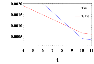
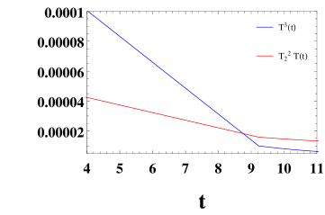
Figure 1: Plot of $T^{2}(t)^{NLO}$ and $T_{1}T(t)^{LO}$ (left fig.) and plot of $T^{3}(t)^{NNLO}$ and $T_{2}^{2}T(t)^{LO}$ (right fig.) versus $t$ for their correosponding $c^{NLO}$ and $c^{NNLO}$ taken to be unity.

NNLO:
Similarly for NNLO, the linearized parameter $T_{2}(<1)$ occurs in the formalism in eqns (49) and (50). For a range between $t_{1}=\ln\frac{Q_{1}^{2}}{\Lambda^{2}}$ to $t_{2}=\ln\frac{Q_{2}^{2}}{\Lambda^{2}}$,

$$T_{2}\propto\frac{<\alpha_{s}(t)^{NNLO}>}{2\pi}=c^{NNLO}\frac{1}{2\pi(t_{2}-t_{1})}\int_{t_{1}}^{t_{2}}\alpha_{s}(t)^{NNLO}dt$$ (71)

As in NLO, the proportionality constant $c^{NNLO}$ is first set as unity. Choosing $t_{1}$ and $t_{2}$ in the $Q$ range $2\leq Q\leq 100$, we obtain we obtain $T_{2}=0.0247$ from eqn.(71). To study the qualitative feature of the linearised relation, we plot fig.(1)(right), and it shows that the linearisation approximation is valid at around small range of $t=8.8$ i.e $Q^{2}=590$ GeV².
We therefore first check the validity of our model around $Q^{2}=590$ GeV² where the NLO and NNLO conditions are valid.

In the previous work [2], $F_{2}^{S(I)}(x,t)$ is preferred over $F_{2}^{S(II)}(x,t)$ within the range of validity of $2\times 10^{-6}\leq x\leq 1\times 10^{-3}$,$2\leq Q\leq 100$ GeV for $\beta=-1.016,K=1.856,\sigma=0.227$. Using the same set of parameters we make our analysis at NLO and NNLO effects first with $T_{1}=0.02704$ and $T_{2}=0.0247$ respectively in the same $x$ and $Q^{2}$ range.

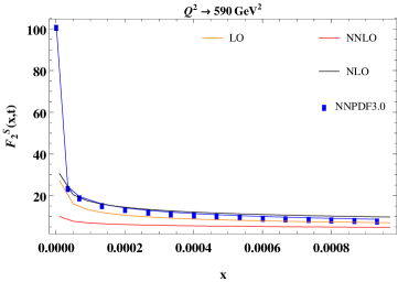
Figure 2: Plots of $F_{2}^{S(I),LO}$ and $F_{2}^{S(I),NLO}$, $F_{2}^{S(I),NNLO}$ as a function of $x$ for fixed $Q^{2}=590$ GeV² and comparison with the NNPDF3.0 data.

In Fig.2 we plot the singlet structure Functions $F_{2}^{S(I),LO}$ and $F_{2}^{S(I),NLO}$, $F_{2}^{S(I),NNLO}$ for a range of small $2\times 10^{-6}\leq x\leq 1\times 10^{-3}$ and at $Q^{2}=590$ GeV² and then compare with the NNPDF3.0 data [29]. We observe that the LO as well as the NLO effects are much closer to data. But when NNLO effects are added the prediction comes below the data.
Changing the values of $T_{1}$ and $T_{2}$ will bring the prediction closer to data. As an illustration we also show for $T_{1}=0.5$ and $T_{2}=10^{-4}$ with the corresponding values of $C^{NLO}=18.491$ and $C^{NNLO}=0.004$ as in fig.(3). At those values of $T_{1}$ and $T_{2}$ the NLO prediction shows a high consistency with the data but we do not observe any significant rise in the evolution for NNLO correction. which interpretes that the parameter $T_{2}$ is is having a very minimal contribution in.

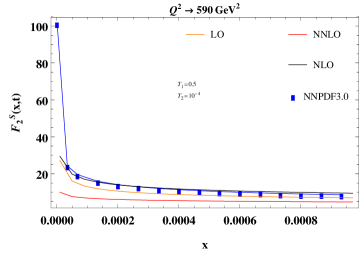
Figure 3: Plots of $F_{2}^{S(I),LO}$ and $F_{2}^{S(I),NLO}$, $F_{2}^{S(I),NNLO}$ as a function of $x$ for fixed $Q^{2}=590$ GeV² using $T_{1}=0.5$ and $T_{2}=10^{-4}$ and comparison with the NNPDF3.0 data.

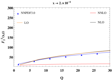
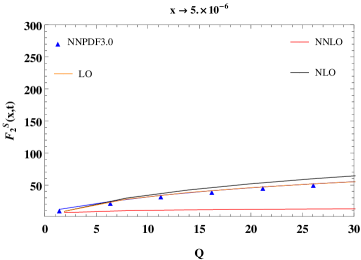
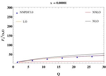
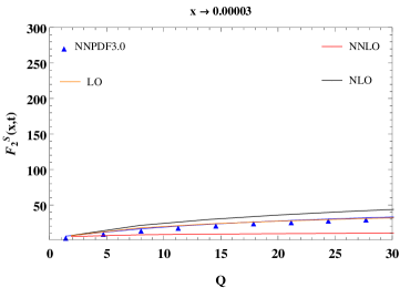
Figure 4: Plots of $F_{2}^{S(I),LO}$ and $F_{2}^{S(I),NLO}$, $F_{2}^{S(I),NNLO}$ as a function of $Q$ for fixed $x$ and comparison with the NNPDF3.0 [29].

In Fig.4 represents the results of $Q$ evolution of the singlet structure Functions $F_{2}^{S(I),LO}$ and $F_{2}^{S(I),NLO}$, $F_{2}^{S(I),NNLO}$ for a few values of small $x$. Using our set of parameters $T_{1}=0.02704$ and $T_{2}=0.0247$ in our models $F_{2}^{S(I),NLO}$ (eqn.33) and $F_{2}^{S(I),NNLO}$ (eqn.52), we compare with the NNPDF3.0 data [29]. We observe that our model upto NLO is valid but when NNLO corrections are taken then the structure function deviates much below the data as well as with the LO and NLO result. This shows that our small $x$ approximations in NLO model is validated than those in our NNLO model.

4 Conclusion

In this paper, we obtained the approximate analytical expressions for the singlet structure functions both at NLO and NNLO from the Taylor approximated coupled DGLAP equations assuming the adhoc $t$ dependent relation between the singlet and the gluon distribution consistent with the analysis of Lopez and Yndurain [13, 20]. At LO the phenomenological analysis is done with the three sets of parameters $\beta=-1.016,K=1.856,\sigma=0.227$ while for NLO and NNLO additional parameters $T_{1}=0.02704$ and $T_{2}=0.0247$ respectively are needed. Our analysis are done around $Q^{2}=590$ GeV² which corresponds to our approximation where our higher order approximation is valid. We make the analysis of both the variation of structure function with $Q$ and $x$.

Let us now conclude this work with a few comments regarding its limitation. There are several approximations which are used to analytically solve the DGLAP equations at small $x$ upto NNLO with valid degree of justification.
(i) The PDFs are expanded at small $x$ (eqn.7) which has inherent theoretical limitations. In DGLAP evolutions, the integrals extends from 0 to 1. Thus at small $x$ one cannot neglect in principle the medium/large $x$ behaviour of the Parton Distribution functions.
(ii) Equation(13) relating the singlet and the Gluon distribution assumes the $x$ dependence of both the distribution to be the same upto a proportionality factor, which may not be true in general. At small scale $(Q^{2})$ the standard PDF available in current literarture Ref.[35] suggest such difference. Even in ultra small $x$ and ultra high $Q^{2}$ double asymptotic scaling limit suggest different $x$ dependence for the singlet and gluon distribution. Specifically at double asymptotic limit (ultra small $x$ and ultra large $Q^{2}$) the corresponding gluon and the singlet distribution have different $x$ dependence in general. [36, 37, 2]. Thus the present assumption appears to be approximately true at limited $x$ and $Q^{2}$ as has been observed in the present work.
(iii) In analytical solutions beyond LO, we need to linearise the $t-$ dependence of the coupling constant $\alpha^{NLO}$ (eqn.(5)) and $\alpha^{NNLO}$ (eqn.(6)). It introduces the parameter $T_{1}$ and $T_{2}$ at NLO and NNLO respectively, which is the inherent limitation of the present analytical approach as had been noted in earlier communication [38, 39]. Such approximations are however found to be true in the limited $Q^{2}$ around 590 GeV².

At the extreme limit of $T_{2}=0$ theoretically we recover the NLO result (as can be observed from eqn.(49) and (50)) but we do not obtain it from the analytical expression (eqn.(67) and (68)), which may predict that the various approximations assumed in solving the DGLAP equations upto NNLO may not be all justified.

Appendix A:

The expressions for the functions $A_{i}^{S}(x,t),B_{i}^{S}(x,t),C_{i}^{S}(x,t),D_{i}^{S}(x,t),L_{i}^{S}(x,t),M_{i}^{S}(x,t)$ where $i=1,2$ involving the integral representation containing the splitting functions as occured in the eqns.(2.2), (2.2) and (2.2), (2.2) are as follows. $A_{i}^{S}(x,t),B_{i}^{S}(x,t),C_{i}^{S}(x,t),D_{i}^{S}(x,t)$ are same in both the cases of NLO and NNLO.

$$A_{1}^{S}(x,t)=\int_{x}^{1}dz\left[P_{qq}^{LO}(x)+2N_{f}P_{qg}^{LO}(x)Kt^{\sigma}\right]$$ (72)

$$B_{1}^{S}(x,t)=\int_{x}^{1}dz\left[P_{qq}^{LO}(x)\frac{x(1-z)}{z}+2N_{f}P_{qg}^{LO}(x)\frac{x(1-z)}{z}Kt^{\sigma}\right]$$ (73)

$$C_{1}^{S}(x,t)=\int_{x}^{1}dz\left[P_{qq}^{NLO}(x)+2N_{f}P_{qg}^{NLO}(x)Kt^{\sigma}\right]$$ (74)

$$D_{1}^{S}(x,t)=\int_{x}^{1}dz\left[P_{qq}^{NLO}(x)\frac{x(1-z)}{z}+2N_{f}P_{qg}^{NLO}(x)\frac{x(1-z)}{z}Kt^{\sigma}\right]$$ (75)

$$A_{2}^{S}(x,t)=\frac{1}{Kt^{\sigma}}\int_{x}^{1}dz\left[P_{gg}^{LO}(x)Kt^{\sigma}+P_{gq}^{LO}(x)\right]$$ (76)

$$B_{2}^{S}(x,t)=\frac{1}{Kt^{\sigma}}\int_{x}^{1}dz\left[P_{gg}^{LO}(x)\frac{x(1-z)}{z}Kt^{\sigma}+P_{gq}^{LO}(x)\frac{x(1-z)}{z}\right]$$ (77)

$$C_{2}^{S}(x,t)=\frac{1}{Kt^{\sigma}}\int_{x}^{1}dz\left[P_{gg}^{NLO}(x)Kt^{\sigma}+P_{gq}^{NLO}(x)\right]$$ (78)

$$D_{2}^{S}(x,t)=\frac{1}{Kt^{\sigma}}\int_{x}^{1}dz\left[P_{gg}^{NLO}(x)\frac{x(1-z)}{z}Kt^{\sigma}+P_{gq}^{NLO}(x)\frac{x(1-z)}{z}\right]$$ (79)

And

$$L_{1}^{S}(x,t)=\int_{x}^{1}dz\left[P_{qq}^{NNLO}(x)+2N_{f}P_{qg}^{NNLO}(x)Kt^{\sigma}\right]$$ (80)

$$M_{1}^{S}(x,t)=\int_{x}^{1}dz\left[P_{qq}^{NNLO}(x)\frac{x(1-z)}{z}+2N_{f}P_{qg}^{NNLO}(x)\frac{x(1-z)}{z}Kt^{\sigma}\right]$$ (81)

$$L_{2}^{S}(x,t)=\frac{1}{Kt^{\sigma}}\int_{x}^{1}dz\left[P_{gg}^{NNLO}(x)Kt^{\sigma}+P_{gq}^{NNLO}(x)\right]$$ (82)

$$M_{2}^{S}(x,t)=\frac{1}{Kt^{\sigma}}\int_{x}^{1}dz\left[P_{gg}^{NNLO}(x)\frac{x(1-z)}{z}Kt^{\sigma}+P_{gq}^{NNLO}(x)\frac{x(1-z)}{z}\right]$$ (83)

Appendix B:

The coefficients $a_{1}(K,t,\sigma),b_{1}(K,t,\sigma),c_{1}(K,t,\sigma),a_{2}(K,t,\sigma),b_{2}(K,t,\sigma),d_{2}(K,t,\sigma),a_{3}(K,t,\sigma),b_{3}(K,t,\sigma),\\ c_{3}(K,t,\sigma),d_{3}(K,t,\sigma),a_{4}(K,t,\sigma),b_{4}(K,t,\sigma),d_{4}(K,t,\sigma)$ as given in eqns.(36)-(39) and the coeffecients $a_{5}(K,t,\sigma),b_{5}(K,t,\sigma),c_{5}(K,t,\sigma),a_{6}(K,t,\sigma),b_{6}(K,t,\sigma),d_{6}(K,t,\sigma),a_{7}(K,t,\sigma),b_{7}(K,t,\sigma),c_{7}(K,t,\sigma),\\ d_{7}(K,t,\sigma),a_{8}(K,t,\sigma),b_{8}(K,t,\sigma),d_{8}(K,t,\sigma)$ as given in eqns.(55)-(58) are listed below.

$$a_{1}(K,t,\sigma,T_{1})=T_{1}(\frac{80}{27}N_{f}+\frac{20}{3}Kt^{\sigma})$$

(84)

$$a_{2}(K,t,\sigma,T_{1})=\frac{8}{3}+\frac{2N_{f}Kt^{\sigma}}{3}+T_{1}.(-435.136-\frac{384217N_{f}}{810}+Kt^{\sigma}(\frac{16\pi^{2}+649}{216}N_{f}+\frac{1219597}{1080}))$$

$$+T_{1}(-3414+\frac{23}{6}Kt^{\sigma})\ln(2)$$

(85)

$$a_{3}(K,t,\sigma,T_{1})=(6+\frac{8}{3Kt^{\sigma}})+T_{1}(\frac{3843}{48}-\frac{61}{9}N_{f}-3\pi^{2}+\frac{1}{Kt^{\sigma}}(\frac{517}{18}-\frac{4}{3}\pi^{2}-\frac{80}{27}N_{f}))$$

(86)

$$a_{4}(K,t,\sigma,T_{1})=(\frac{11}{12}-\frac{N_{f}}{3}-11)-\frac{12}{Kt^{\sigma}}-T_{1}(\frac{20035}{3601}+\frac{7\pi^{2}}{2}-\frac{679705.51}{1320}+\frac{1}{Kt^{\sigma}}(\frac{80}{27}N_{f}+\frac{11\pi^{2}}{3}$$

$$+\frac{2317}{864}+\frac{103837.66}{81})+T_{1}(\frac{45}{2})$$ (87)

$$a_{5}(K,t,\sigma,T_{2})=T_{2}(\frac{80N_{f}}{27}+\frac{20Kt^{\sigma}}{3})+T_{2}^{2}(-19666.936+38600.48Kt^{\sigma})$$ (88)

$$a_{6}(K,t,\sigma,T_{2})=\frac{8}{3}+\frac{2N_{f}Kt^{\sigma}}{3}+T_{2}(-435.136-\frac{384217N_{f}}{810})+T_{2}(-3414+\frac{23}{6}Kt^{\sigma})\ln(2)$$

$$+T_{2}^{2}(4061.071-3921.587\times 8Kt^{\sigma})$$ (89)

$$a_{7}(K,t,\sigma,T_{2})=(6+\frac{8}{3Kt^{\sigma}})+T_{2}\left(\frac{3843}{48}-\frac{61N_{f}}{9}-3\pi^{2}+\frac{1}{Kt^{\sigma}}(\frac{517}{18}-\frac{4\pi^{2}}{3}-\frac{80N_{f}}{27})\right)$$

$$+T_{2}^{2}(135983.174+\frac{3240.749}{Kt^{\sigma}})$$ (90)

$$a_{8}(K,t,\sigma,T_{1})=(\frac{11}{12}-\frac{N_{f}}{3}-11)-\frac{12}{Kt^{\sigma}}-T_{1}(\frac{20035}{3601}+\frac{7\pi^{2}}{2}-\frac{679705.51}{1320}+\frac{1}{Kt^{\sigma}}(\frac{80}{27}N_{f}+\frac{11\pi^{2}}{3}$$

$$+\frac{2317}{864}+\frac{103837.66}{81})+T_{1}(\frac{45}{2})+T_{2}^{2}(-87979.883-\frac{28540.98}{Kt^{\sigma}})$$

(91)

$$b_{1}(K,t,\sigma,T_{1})=-\frac{5}{3}N_{f}Kt^{\sigma}+T_{1}(\frac{416151}{324}N_{f}-\frac{627740.73}{5832}+Kt^{\sigma}(\frac{1659953}{2160}+\frac{\pi^{2}}{27})+(-\frac{204}{81}-\frac{883}{4}Kt^{\sigma})\ln(2))$$

(92)

$$b_{2}(K,t,\sigma,T_{1})=(\frac{4}{3}-N_{f}Kt^{\sigma})+T_{1}(\frac{-16791.29}{12}+\frac{3593N_{f}}{108}+\frac{125Kt^{\sigma}}{16})$$

(93)

$$b_{4}(K,t,\sigma,T_{1})=\frac{1}{Kt^{\sigma}}(12Kt^{\sigma}+16)+T_{1}(\frac{679}{108}N_{f}-\frac{2305}{32}-4\pi^{2}-\frac{1}{Kt^{\sigma}}(\frac{79649}{81}-\frac{4\pi^{2}}{3}-\frac{128}{27}N_{f}))$$

$$b_{5}(K,t,\sigma,T_{2})=-\frac{5}{3}N_{f}Kt^{\sigma}+T_{2}\left(\frac{416151N_{f}}{324}-\frac{627740.73}{5832}+Kt^{\sigma}(\frac{1659953}{2160}+\frac{\pi^{2}}{27})\right)$$

$$+T_{2}\left(-\frac{204}{81}\ln(2)-\frac{883}{4}Kt^{\sigma}\ln(2)\right)+T_{2}^{2}\left(-12075.005-329142.4Kt^{\sigma}\right)$$ (94)

$$b_{6}(K,t,\sigma,T_{2})=(\frac{4}{3}-N_{f}Kt^{\sigma})+T_{2}(\frac{-16791.29}{12}+\frac{3593N_{f}}{108}+\frac{125Kt^{\sigma}}{16})+T_{2}^{2}(-2143.669-22467.4$$

$$\times 8Kt^{\sigma})$$ (95)

$$b_{7}(K,t,\sigma,T_{2})=(8+\frac{2}{3Kt^{\sigma}})+T_{2}\left(\frac{989}{108}N_{f}+4\pi^{2}+\frac{2557}{32}-\frac{20}{Kt^{\sigma}}\right)+T_{2}\left(\frac{1}{Kt^{\sigma}}(\frac{5104}{81}+4\pi^{2}+\frac{208}{27}N_{f})\right)$$

$$+T_{2}^{2}(-139453.698-\frac{22436.898}{Kt^{\sigma}})$$ (96)

$$b_{8}(K,t,\sigma,T_{2})=\frac{1}{Kt^{\sigma}}(12Kt^{\sigma}+16)+T_{2}(\frac{679}{108}N_{f}-\frac{2305}{32}-4\pi^{2}-\frac{1}{Kt^{\sigma}}(\frac{79649}{81}-\frac{4\pi^{2}}{3}-\frac{128}{27}N_{f}))$$

$$+T_{2}^{2}(49919.486+\frac{19159.5}{Kt^{\sigma}})$$

(97)

$$c_{1}(K,t,\sigma,T_{1})=T_{1}(\frac{39634.98}{144}-\frac{158355}{4374}N_{f}+Kt^{\sigma}(\frac{395}{216}N_{f}-\frac{1533}{144}))$$

(98)

$$c_{5}(K,t,\sigma,T_{2})=T_{2}(\frac{39634.98}{144}-\frac{158355}{4374}N_{f}+Kt^{\sigma}(\frac{395}{216}N_{f}-\frac{1533}{144}))+T_{2}^{2}(3866.215$$

$$+218339.68Kt^{\sigma})$$

(99)

$$c_{7}(K,t,\sigma,T_{2})=(-12+\frac{16}{3Kt^{\sigma}})-T_{2}\left\{\frac{989}{108}N_{f}+4\pi^{2}+\frac{2557}{32}-\frac{20}{Kt^{\sigma}}\right\}+$$

$$T_{2}\left\{\frac{1}{Kt^{\sigma}}\left(\frac{5104}{81}+4\pi^{2}+\frac{208}{27}N_{f}\right)\right\}+T_{2}^{2}\left\{-139453.698-\frac{22436.898}{Kt^{\sigma}}\right\}$$ (100)

$$d_{2}(K,t,\sigma,T_{1})=T_{1}(\frac{80}{27}N_{f}+\frac{20}{3}Kt^{\sigma})$$

$$d_{4}(K,t,\sigma,T_{1})=\frac{1}{KT^{\sigma}}(KT^{\sigma}+\frac{8}{3})+T_{1}\left(\frac{3843}{48}-\frac{61}{9}N_{f}-3\pi^{2}+\frac{1}{KT^{\sigma}}(\frac{517}{18}-\frac{4\pi^{2}}{3}-\frac{80}{27}N_{f})\right)$$ (101)

$$d_{6}(K,t,\sigma,T_{2})=T_{2}(\frac{80}{27}N_{f}+\frac{20}{3}Kt^{\sigma})+T_{2}^{2}(-1908740+4825.06\times 8Kt^{\sigma})$$

(102)

$$d_{8}(K,t,\sigma,T_{2})=\frac{1}{KT^{\sigma}}(KT^{\sigma}+\frac{8}{3})+T_{2}\left(\frac{3843}{48}-\frac{61}{9}N_{f}-3\pi^{2}+\frac{1}{KT^{\sigma}}(\frac{517}{18}-\frac{4\pi^{2}}{3}-\frac{80}{27}N_{f})\right)$$

$$+T_{2}^{2}(135983.313-\frac{3240.75}{Kt^{\sigma}})$$

(103)

$$d_{3}(K,t,\sigma,T_{1})=T_{1}\frac{45}{2}$$

(104)

$$d_{7}(K,t,\sigma,T_{2})=T_{2}\frac{45}{2}$$