BOSH: Bayesian Optimization by Sampling Hierarchically

Abstract

Deployments of Bayesian Optimization (BO) for functions with stochastic evaluations, such as parameter tuning via cross validation and simulation optimization, typically optimize an average of a fixed set of noisy realizations of the objective function. However, disregarding the true objective function in this manner finds a high-precision optimum of the wrong function. To solve this problem, we propose Bayesian Optimization by Sampling Hierarchically (BOSH), a novel BO routine pairing a hierarchical Gaussian process with an information-theoretic framework to generate a growing pool of realizations as the optimization progresses. We demonstrate that BOSH provides more efficient and higher-precision optimization than standard BO across synthetic benchmarks, simulation optimization, reinforcement learning and hyper-parameter tuning tasks.

1 Introduction

Bayesian Optimization (BO) (Mockus, 2012) is a well-studied global optimization routine for finding the optimizer $\textbf{x}^{*}$ of a ‘smooth’ but expensive-to-evaluate function $g$ across a compact domain $\mathcal{X}\subset\mathds{R}^{d}$. BO is particularly popular for problems where we have access to only noisy evaluations of $g$ and has had many successful applications optimizing high-cost stochastic functions, including fine-tuning machine learning (ML) models (Snoek et al., 2012), optimizing simulations in operational research (Kleijnen, 2009), and designing experiments in the physical sciences (Frazier and Wang, 2016).

For many stochastic optimization tasks, it is commonplace to disregard the original objective function $g$ and instead optimize the average of a collection of $K$ specific realizations $f_{s}$. Common examples include the $K$ data partitions used to estimate ML model performance through $K$-fold Cross Validation (CV) (Kohavi, 1995) or considering $K$ fixed initial conditions to create sample average approximations for simulation optimization and reinforcement learning (Kleywegt et al., 2002). This small collection of realization indexed by $S=\{s_{1},..s_{K}\}$ is typically randomly initialized, but then fixed for the remainder of the optimization. We henceforth refer to $S$ as an evaluation strategy, with its optimization seeking $\textbf{x}_{S}^{*}=\operatorname*{argmax}_{\textbf{x}\in\mathcal{X}}\tilde{g}_{S}(\textbf{x})$, where $\tilde{g}_{S}(\textbf{x})=\frac{1}{K}\sum_{i=1}^{K}f_{s_{i}}(\textbf{x})$.

Evaluations of $\tilde{g}_{S}(\textbf{x})$ enjoy a substantial reduction in variance compared to a single stochastic evaluation of the true objective function $g(\textbf{x})$. However, there is no guarantee that $\textbf{x}^{*}_{S}\approx\textbf{x}^{*}$, as $\textbf{x}^{*}_{S}$ is a function of the randomly selected $S$. In fact, estimators of this form are well-studied in the robust statistics literature (Hampel et al., 2011), where it is known that the expected suboptimality $\mathds{E}_{S}[g(\textbf{x}^{*})-g(\textbf{x}_{S}^{*})]$ is a positive quantity decaying as $O(\frac{1}{K})$. Regardless of the sophistication of our optimization routine, if $K$ is set too low we cannot optimize $g$ to an arbitrary precision level by optimizing $\tilde{g}_{S}$. In contrast, as each individual evaluation of $\tilde{g}_{S}$ costs $K$ times that of evaluating $g$, setting $K$ too large wastes computational resources on unnecessarily expensive evaluations. Therefore, as demonstrated for hyper-parameter tuning (Moss et al., 2018), model selection (Moss et al., 2019) and simulation optimization (Kim et al., 2015), the efficiency and effectiveness of a fixed evaluation strategy crucially depends on the choice of $K$.

To avoid the need for fixed evaluation strategies, we propose BOSH (Bayesian Optimization by Sampling Hierarchically), the first BO routine that maintains and grows a pool of realizations as the optimization progresses. A Hierarchical Gaussian Process (HGP) (Hensman et al., 2013) is used to quantify uncertainty in our current evaluation strategy by modeling different realizations as separate perturbations of the latent ‘true’ object function (Figure 1). A novel information-theoretic framework then uses the HGP’s predictions to balance the utility of making further evaluations in the current pool $\{f_{s}\}_{s\in S}$ against the benefit of considering a new realization $f_{s^{*}}$.

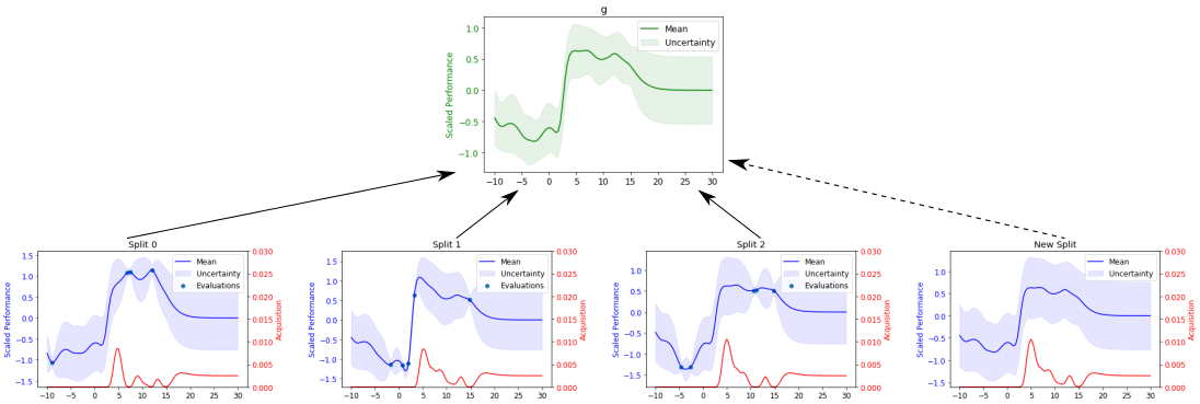
Figure 1: Tuning an SVM hyper-parameter on IMDB data using BOSH. Evaluations across three train-test splits (blue) are aggregated to predict the true accuracy (green) and the likely behavior of a new train-test split (right-most panel). The utility of making a new evaluation on each of the considered splits (red) is lower around locations already evaluated on another train-test split.

2 Related Work

Using low-cost approximations to speed up optimization is well-studied. Multi-task (Swersky et al., 2013; Poloczek et al., 2017, MT) and multi-fidelity (Kandasamy et al., 2016; Lam et al., 2015; McLeod et al., 2017; Wu and Frazier, 2018; Takeno et al., 2019, MF) BO provides efficient optimization for problems where low-cost alternative functions hold some relationship with the true objective function. A popular application is hyper-parameter tuning (Klein et al., 2017; Kandasamy et al., 2017; Falkner et al., 2018), where dataset size is controlled to provide fast but rough tuning. The closest MT framework to BOSH is FASTCV (Swersky et al., 2013), which speeds up hyper-parameter tuning under fixed evaluation strategies by choosing to evaluate individual $K$ train-test splits making up $K$-fold CV. However, FASTCV’s coregionalisation kernel cannot predict performance on previously unobserved splits or support an adaptive evaluation strategy. To guarantee high-precision optimization, a large choice of $K$ must be chosen a-priori, incurring substantial initialization costs and slower optimization. Furthermore, these approaches are unable to recommend batches of points, and it is unclear how to apply existing batch heuristics, for example González et al. (2016), to MF or MT frameworks.

Parallel work of Pearce et al. (2019) from the operational research literature address a similar problem but in a different way; reducing simulation stochasticity by exploiting common random numbers. Similarly to BOSH, performance is measured according to individual random samples. However, their model is complex and challenging to fit, and their search strategy incurs a computational overhead that grows exponentially with the dimensions of the search space. In contrast, our framework makes principled decisions with a linearly scaling cost and is able to recommend batches.

3 BOSH

The key difference between BOSH and existing BO is that instead of only modeling $\tilde{g}_{S}$ for a fixed evaluation strategy $S$, BOSH separately models individual realizations $f_{s}$. By assuming that each $f_{s}$ is some perturbation of the true objective function $g$ (see Fig. 1), we can fit a hierarchical model that learns the correlations between $g$ and each $f_{s}$. Knowledge of this correlation structure provides information about the likely behavior of a yet unobserved realization $f_{s^{*}}$. Therefore, BOSH can make principled decisions about which realization to use for the next evaluation from the set of candidate realizations $\{f_{s}\}_{s\in S^{*}}$, where $S^{*}=S\cup\{s^{*}\}$ — either a realization from the current evaluation strategy $S$ or generating a new realization $f_{s^{*}}$ (to be absorbed into $S$ for subsequent optimization steps). This allows BOSH to target $g$ directly, instead of targeting just $\tilde{g}_{S}$.

Like most BO frameworks, BOSH has two key components: a Gaussian Process (GP) (Rasmussen, 2004) surrogate model predicting the values of not-yet-evaluated points, and an acquisition function using these predictions to efficiently explore the search space. For BOSH, we require an acquisition function $\alpha$ estimating the utility of evaluating any $\textbf{x}\in\mathcal{X}$ on any realization $f_{s}$ for $s\in S^{*}$. After collecting $n$ (potentially noisy) evaluations, BOSH evaluates locations on realizations that score highly according to the acquisition function, repeating until the optimization budget is exhausted.

3.1 The BOSH Surrogate Model

A natural framework for modeling function realizations as perturbations of a true objective function is a Hierarchical Gaussian Process (HGP) (Hensman et al., 2013), where the true objective function is modeled as a GP with an ‘upper’ kernel $k_{g}$, and the deviations to all the individual realizations $f_{s}$ modeled by another GP with a ‘lower’ kernel $k_{f}$. As is common in BO, we use Matérn 5/2 kernels (Matérn, 1960). The HGP structure is equivalently understood as each $f_{s}$ being a conditionally independent GPs with shared mean function $g$, i.e.

$$y_{i}=f_{s_{i}}(\textbf{x}_{i})+\epsilon_{i}\quad\text{for}\quad f_{s}\sim\mathcal{GP}(g,k_{f})\quad\text{where}\quad g\sim\mathcal{GP}(0,k_{g}),$$

for $\epsilon_{i}\stackrel{{\scriptstyle\rm i.i.d}}{{\sim}}\mathcal{N}(0,\sigma^{2})$. This induces a prior covariance structure of

$$Cov(f_{s}(\textbf{x}),f_{s^{\prime}}(\textbf{x}^{\prime})))=k_{g}(\textbf{x},\textbf{x}^{\prime})+\mathds{I}_{s=s^{\prime}}k_{f}(\textbf{x},\textbf{x}^{\prime})\quad\text{and}\quad Cov(f_{s}(\textbf{x}),g(\textbf{x}^{\prime}))=k_{g}(\textbf{x},\textbf{x}^{\prime}),$$

where $\mathds{I}$ is an indicator function. Samples from this prior are provided in Fig. 2. Crucially, given observations $D_{n}=\{(\textbf{x}_{i},s_{i},y_{i})\}_{i=1}^{n}$, the HGP provides a bi-variate Gaussian joint distribution for $(y_{s}(\textbf{x}),g(\textbf{x}))\,|\,D_{n}$, the quantities required to evaluate our acquisition function (see below). Prediction cost is equivalent to a standard GP, with the $n^{th}$ BO step dominated by an $O(n^{3})$ matrix inversion.

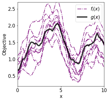
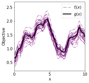
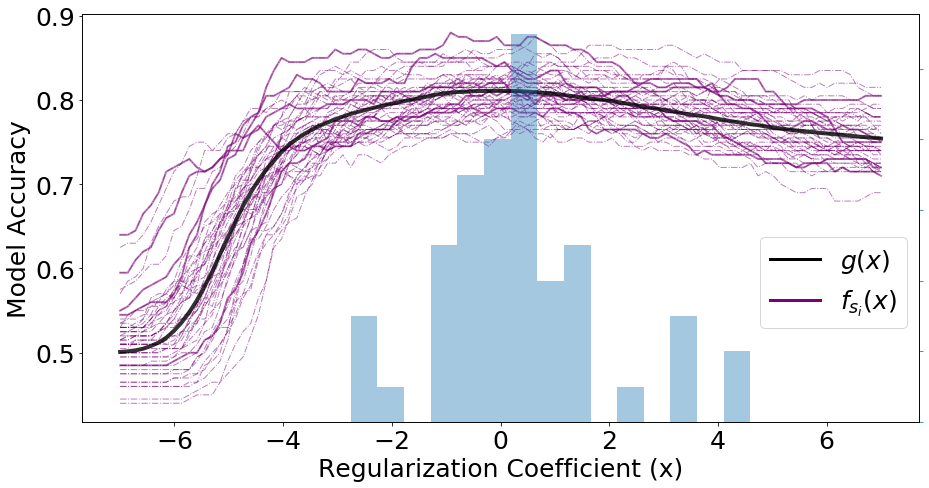
Figure 2: (left) and (middle) show samples from HGPs with different lower kernels, demonstrating a capacity for modeling real scenarios like the performance estiamted by train-test splits when tuning regularization of a logistic regression sentiment classifier of IMDB movie reviews (right). Purple lines show sampled $f_{s}(x)$ and the true objective $g(x)$ is plotted in black (as calculated on a large independent test set). The histogram of chosen regularization (performance curve maxima) shows many splits choosing highly suboptimal regularization ($-4\%$ accuracy).

3.2 The BOSH Acquisition Function

We base our acquisition function on the max-value entropy search of Wang and Jegelka (2017), which seeks to reduce uncertainty in the optimal value $g^{*}=g(\textbf{x}^{*})$. As is common in the BO literature (Hennig and Schuler, 2012; Hernández-Lobato et al., 2014), we measure uncertainty in terms of the differential entropy of our current belief about the maximum value, given by $H(g^{*})=-\mathds{E}_{g\sim p_{g^{*}}}\left(\log p_{g^{*}}(g)\right)$, where $p_{g*}$ is the probability density function of $g^{*}|D_{n}$ according to our HGP. The reduction in entropy of $g^{*}$ provided by a batch of $B$ evaluations $\{y_{s_{j}}(\textbf{x}_{j})\}_{j=1}^{B}$ is measured as their mutual information $I$, defined as

$$I(g^{*};\{y_{s_{j}}(\textbf{x}_{j})\}_{j=1}^{B}|D_{n})\coloneqq H(\{y_{s_{j}}(\textbf{x}_{j})\}_{j=1}^{B}|D_{n})-\mathds{E}_{g^{*}|D_{n}}\left[H(\{y_{s_{j}}(\textbf{x}_{j})\}_{j=1}^{B}|g^{*},D_{n})\right].$$ (1)

Defining $\textbf{z}_{i}=(\textbf{x}_{i},s_{i})$, principled batch BO corresponds to selecting $\{\textbf{z}_{i}\}_{i=1}^{B}$ to maximize (1).

Unfortunately, neither $g^{*}|D_{n}$ nor the differential entropy of $y_{s}(\textbf{x}|g^{*},D_{n})$ have closed-form expressions. Therefore, to implement information-theoretic BO, the second term of (1) must be approximated. The MUMBO (MUlti-task Max-value Bayesian Optimization) acquisition function (Moss et al., 2020) provides one such approximation when $B=1$, requiring only simple single-dimensional numerical integrations regardless of the dimensions of the search space. To extend MUMBO beyond $B>1$, we make an additional approximation through a well-known information-theoretic inequality — that the joint differential entropy of a collection of random variables is upper-bounded by the individual entropies. BOSH’s acquisition function is the resulting lower bound, expressed in terms of the MUMBO acquisition function as

$$\alpha_{n}^{BOSH}(\{\textbf{z}_{j}\}_{j=1}^{B})=\frac{1}{2}\log\left(|\textbf{C}_{n}(\{\textbf{z}_{j}\}_{j=1}^{B})|\right)+\sum_{j=1}^{B}\alpha^{MUMBO}_{n}(\textbf{z}_{j}),$$ (2)

where $\textbf{C}_{n}$ is the HGP’s predictive correlation matrix between each of the $B$ batch elements. The first term of (2) encourages diversity (achieving high values for batches with low posterior correlation) whereas the second term encourages evaluations in areas providing large amounts of information about $g^{*}\,|\,D_{n}$. As the $B\times d$-dimensional maximization of (2) posed too great a computational challenge, we greedily construct batches with $B$ separate sequential decisions, each performed with the DIRECT maximizer (Jones, 2009). An extended publication (currently in submission) explores the relationship between (2) and determinantal point processes (e.g. Kulesza et al., 2012).

4 Experiments

All our experiments show that fixed evaluation strategies can provide either precise or efficient optimization of stochastic objective functions, whereas BOSH achieves both. We compare BOSH against standard BO using two popular acquisition functions: expected improvement (EI) (Mockus et al., 1978) and max-value entropy search (MES) (Wang and Jegelka, 2017). We also consider FASTCV (Swersky et al., 2013), and, for our hyper-parameter tuning tasks, FABOLAS (Klein et al., 2017). Code built upon the Emukit Python package (Paleyes et al., 2019) is provided, alongside additional experimental details, at redacted for review. For a fair reflection of parallel computing resources, evaluations of whole batches (or evaluation strategy) are recorded as a single BO step. We compare the performance of BOSH producing batches of size $B$ against the performance of standard BO using evaluation strategies of $K=B$ fixed realizations as well as $B$ realizations re-sampled at each BO step. We plot the mean suboptimality and one standard error across 100 repetitions.

BOSH’s ability to evaluate diverse batches of points in parallel instead of single locations across a whole evaluation strategy provides a natural advantage over standard BO, particularly in the early stages of optimization. Therefore, to explicitly disentangle the benefits of BOSH’s adaptive evaluation strategy from its ability to recommend batches, we also consider standard BO recommending batches across an evaluation strategy consisting of a single fixed realization. We present the performance of batch BO choosing $B$ evaluations across a single fixed realization, considering both the popular locally penalized (LP) EI (González et al., 2016) as well as our proposed batch approximation applied to a MES acquisition function (instead of MUMBO). Note that FASTCV and FABOLAS do not support batches. We do not consider simultaneously deploying both batch BO and full evaluation strategies, as this is beyond the resources of most ML researchers.

For GP initialization, we randomly sample one more evaluation than kernel parameters (to guarantee identifiability). For standard BO, this corresponds to d+3 evaluations of the chosen evaluation strategy (i.e K*(d+3) individual evaluations). For BOSH, rather than using separate lower and upper kernels for our HGP, we found that sharing length-scales between each kernel greatly improved the stability of the HGP and allowed reliable initialization after just d+5 evaluations across an initial pair of realizations. Reliable initialization of FASTCV’s K*K correlation matrix entries (of which its performance was sensitive) required at least d+3 evaluations for each of its K realizations. Therefore, as well as providing improved efficiency and precision once optimization begins, BOSH’s ability to model only as many individual realizations as required allows significantly lower initialization costs.

Synthetic Objective (d=1). First, we simulate data directly from an HGP (Figure 4) and seek to find the maximum of $g(x)$ (as plotted in Figure 2) by querying only the perturbed curves $f_{s}$. We consider two different lower kernels, one with a smaller variance ( $V$) causing low between-realization variability, and another with a larger variance causing high between-realization variability.

Reinforcement Learning (d=7). BOSH can fine-tune the $7$ parameters directing a lunar lander module to its landing zone ( provided by OpenAI Gym https://gym.openai.com/envs/LunarLander-v2/). A particular configuration is tested by running a single (or $B$) randomly generated scenarios. We seek to outperform OpenAI’s hard-coded controller (denoted PID ) according to ‘true’ performance over a set of $100$ specific initial conditions, using as few simulation runs as possible (Figure 4).

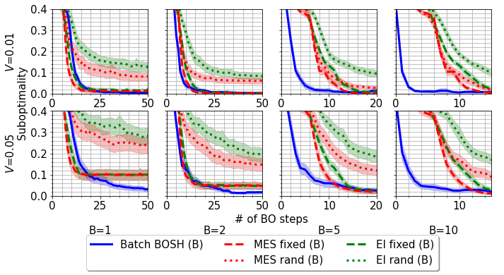
Figure 3: Maximizing the upper functions of two HGPs with differing lower kernel variances ($V$) across a range of evaluation strategy sizes ($B$). BOSH’s optimization is more efficient (precise) than BO on large (small) evaluation strategies

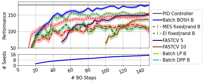
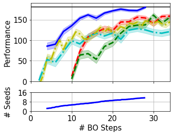
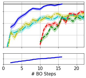
Figure 4: Maximizing Lunar Lander performance with B=1,5,10 (upper, left, right). BOSH adaptively considers up to $15$ realizations and can match the performance of the PID controller.

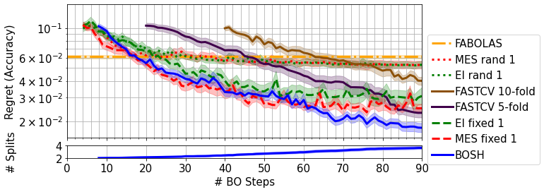
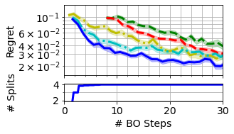
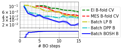
Figure 5: Minimizing SVM error for IMDB movie review classification with B=1,5,10 (upper, left, right). BOSH considers up to four realizations to provide higher-precision tuning than standard BO. When parallel resources are available, BOSH provides faster tuning than BO under CV and more precise tuning than batch BO.

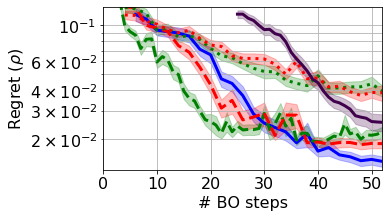
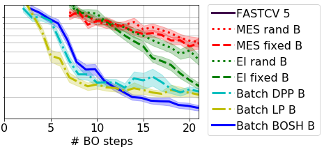
Figure 6: Allocating warehouses to cope with demand for B=1,5 (upper, lower). Although standard BO provides fast rough optimization, only BOSH achieves high-precision optimization.

Hyper-parameter Tuning (d=2). BOSH can also be used to tune the hyper-parameters of ML models, e.g. the two hyper-parameters of an SVM classifying IMDB movie review sentiment (Figure 6). During tuning, BOSH uses a pool of train-test splits and standard BO uses fixed evaluation strategies of single train-test splits or $K$-fold CV. True performance is calculated retrospectively on a large held-out test set. Although finding a reasonable configuration after a very small optimization budget, FABOLAS’s reliance on low-fidelity estimates prevents precise optimization.

Simulation Optimization (d=4). Our final experiment (Figure 6) considers a simulation optimization problem from the set of benchmarks of http://simopt.org/. We wish to decide $(x,y)$ locations of two warehousing facilities. Orders arise according to a pre-specified non-homogeneous Poisson process and each order is served by one of the ten trucks belonging to the closest warehouse (or queued if all trucks are busy). The goal is to maximize the proportion $\rho$ of orders delivered within $60$ minutes. Base estimate of $\rho$ comes from simulating demand for a single day according to a single random seed. We can calculate more reliable estimates by simulating demand for $B$ independent days and we retrospectively estimate the true $\rho$ with an expensive but reliable $100$ day simulation.

References

- Falkner et al. (2018) Stefan Falkner, Aaron Klein, and Frank Hutter. Bohb: Robust and efficient hyperparameter optimization at scale. arXiv preprint arXiv:1807.01774, 2018.
- Frazier and Wang (2016) Peter I Frazier and Jialei Wang. Bayesian optimization for materials design. In Information Science for Materials Discovery and Design, pages 45–75. Springer, 2016.
- González et al. (2016) Javier González, Zhenwen Dai, Philipp Hennig, and Neil Lawrence. Batch Bayesian optimization via local penalization. In Artificial intelligence and statistics, pages 648–657, 2016.
- Hampel et al. (2011) Frank R Hampel, Elvezio M Ronchetti, Peter J Rousseeuw, and Werner A Stahel. Robust Statistics: The Approach Based on Influence Functions. John Wiley & Sons, 2011.
- Hennig and Schuler (2012) Philipp Hennig and Christian J Schuler. Entropy search for information-efficient global optimization. Journal of Machine Learning Research, 13:1809–1837, 2012.
- Hensman et al. (2013) James Hensman, Neil D Lawrence, and Magnus Rattray. Hierarchical Bayesian modelling of gene expression time series across irregularly sampled replicates and clusters. BMC Bioinformatics, 14:252, 2013.
- Hernández-Lobato et al. (2014) José Miguel Hernández-Lobato, Matthew W Hoffman, and Zoubin Ghahramani. Predictive entropy search for efficient global optimization of black-box functions. In Neural Information Processing Systems, 2014.
- Jones (2009) Donald R Jones. Direct global optimization algorithm. Encyclopedia of optimization, 1(1):431–440, 2009.
- Kandasamy et al. (2016) Kirthevasan Kandasamy, Gautam Dasarathy, Junier B Oliva, Jeff Schneider, and Barnabás Póczos. Gaussian process bandit optimisation with multi-fidelity evaluations. In Neural Information Processing Systems, 2016.
- Kandasamy et al. (2017) Kirthevasan Kandasamy, Gautam Dasarathy, Jeff Schneider, and Barnabás Póczos. Multi-fidelity Bayesian optimisation with continuous approximations. In International Conference in Machine Learning, 2017.
- Kim et al. (2015) Sujin Kim, Raghu Pasupathy, and Shane G Henderson. A guide to sample average approximation. In Handbook of simulation optimization, pages 207–243. Springer, 2015.
- Kleijnen (2009) Jack PC Kleijnen. Kriging metamodeling in simulation: A review. European journal of operational research, 192(3):707–716, 2009.
- Klein et al. (2017) Aaron Klein, Stefan Falkner, Simon Bartels, Philipp Hennig, and Frank Hutter. Fast Bayesian optimization of machine learning hyperparameters on large datasets. International Conference on Artificial Intelligence and Statistics, 2017.
- Kleywegt et al. (2002) Anton J Kleywegt, Alexander Shapiro, and Tito Homem-de Mello. The sample average approximation method for stochastic discrete optimization. SIAM Journal on Optimization, 12(2):479–502, 2002.
- Kohavi (1995) Ron Kohavi. A study of cross-validation and bootstrap for accuracy estimation and model selection. In International Joint Conference on Artificial Intelligence, 1995.
- Kulesza et al. (2012) Alex Kulesza, Ben Taskar, et al. Determinantal point processes for machine learning. Foundations and Trends® in Machine Learning, 5(2–3):123–286, 2012.
- Lam et al. (2015) Rémi Lam, Douglas L Allaire, and Karen E Willcox. Multifidelity optimization using statistical surrogate modeling for non-hierarchical information sources. In Structures, Structural Dynamics, and Materials Conference, 2015.
- Matérn (1960) Bertil Matérn. Spatial variation, volume 36 of. Lecture Notes in Statistics, 1960.
- McLeod et al. (2017) Mark McLeod, Michael A Osborne, and Stephen J Roberts. Practical Bayesian optimization for variable cost objectives. arXiv preprint arXiv:1703.04335, 2017.
- Mockus (2012) Jonas Mockus. Bayesian approach to global optimization: theory and applications, volume 37. Springer Science & Business Media, 2012.
- Mockus et al. (1978) Jonas Mockus, Vytautas Tiesis, and Antanas Zilinskas. The application of bayesian methods for seeking the extremum. Towards global optimization, 2(117-129):2, 1978.
- Moss et al. (2018) Henry B. Moss, David S. Leslie, and Paul Rayson. Using J-K-fold cross validation to reduce variance when tuning nlp models. In International Conference on Computational Linguistics, 2018.
- Moss et al. (2019) Henry B. Moss, Andrew Moore, David L. Leslie, and Paul Rayson. FIESTA: Fast IdEntification of State-of-The-Art models using adaptive bandit algorithms. In Proceedings of the 57th Annual Meeting of the Association for Computational Linguistics, 2019.
- Moss et al. (2020) Henry B. Moss, David S. Leslie, and Paul Rayson. MUMBO: Multi-task Max-value Bayesian Optimization. In Joint European Conference on Machine Learning and Knowledge Discovery in Databases, 2020.
- Paleyes et al. (2019) Andrei Paleyes, Mark Pullin, Maren Mahsereci, Neil Lawrence, and Javier González. Emulation of physical processes with emukit. In Second Workshop on Machine Learning and the Physical Sciences, NeurIPS, 2019.
- Pearce et al. (2019) Michael Pearce, Matthias Poloczek, and Juergen Branke. Bayesian optimization allowing for common random numbers. arXiv preprint arXiv:1910.09259, 2019.
- Poloczek et al. (2017) Matthias Poloczek, Jialei Wang, and Peter Frazier. Multi-information source optimization. In Neural Information Processing Systems, 2017.
- Rasmussen (2004) Carl Edward Rasmussen. Gaussian processes in machine learning. In Advanced Lectures on Machine Learning, pages 63–71. Springer, 2004.
- Snoek et al. (2012) Jasper Snoek, Hugo Larochelle, and Ryan P Adams. Practical Bayesian optimization of machine learning algorithms. In Neural Information Processing Systems, 2012.
- Swersky et al. (2013) Kevin Swersky, Jasper Snoek, and Ryan P Adams. Multi-task Bayesian optimization. In Neural Information Processing Systems, 2013.
- Takeno et al. (2019) Shion Takeno, Hitoshi Fukuoka, Yuhki Tsukada, Toshiyuki Koyama, Motoki Shiga, Ichiro Takeuchi, and Masayuki Karasuyama. Multi-fidelity bayesian optimization with max-value entropy search. arXiv preprint arXiv:1901.08275, 2019.
- Wang and Jegelka (2017) Zi Wang and Stefanie Jegelka. Max-value entropy search for efficient Bayesian optimization. In International Conference in Machine Learning, 2017.
- Wu and Frazier (2018) Jian Wu and Peter I Frazier. Continuous-fidelity bayesian optimization with knowledge gradient. 2018.