Robust MPC for Linear Systems with Parametric and Additive Uncertainty:
A Novel Constraint Tightening Approach

Abstract

We propose a novel approach to design a robust Model Predictive Controller (MPC) for constrained uncertain linear systems. The uncertain system is modeled as linear parameter varying with additive disturbance. Set bounds for the system matrices and the additive uncertainty are assumed to be known. We formulate a novel optimization-based constraint tightening strategy around a predicted nominal trajectory which utilizes these bounds. With an appropriately designed terminal cost function and constraint set, we prove robust satisfaction of the imposed constraints by the resulting MPC in closed-loop with the uncertain system, and Input to State Stability of the origin. We highlight the efficacy of our proposed approach via a numerical example.

1 Introduction

Model Predictive Control (MPC) is a well established optimal control strategy that is able to handle imposed constraints on system states and inputs [25]. The MPC approach is based on solving a constrained finite horizon optimal control problem at each time step and applying the first optimal input to the plant. A key challenge in MPC design is to guarantee robust constraint satisfaction in the presence of uncertainty in the prediction model.

For uncertain linear systems in presence of only an additive disturbance, finding the optimal policy is NP-hard and typically involves dynamic programming [7, Chapter 15],[31, Chapter 3], or Min-Max feedback [33, 3] approaches. Computationally tractable suboptimal robust MPC techniques such as tube MPC [12, 16, 28] are well understood and widely used. The key idea is to restrict the input policy to affine or piecewise affine state feedback policies and then tighten the state constraints so that all trajectories within a “tube” satisfy the imposed state constraints for all possible disturbances.

On the other hand, robust MPC design for uncertain linear systems in presence of both a mismatch in the system dynamics matrices and an additive disturbance is more involved and is a topic of active research [11, 1]. Min-Max MPC strategies could be computed in this case, but their computational complexity scales exponentially with the prediction horizon. Restricting the input policy parametrization to affine state feedback policies leads to computationally tractable ellipsoidal regions of attraction (ROA) [6]. Such methods are presented in [18, 20]. Polytopic, homothetic and elastic tube MPC methods with affine or piecewise affine state feedback policy parametrizations are introduced in [21, 26, 30] to address the conservatism inherent to ellipsoidal ROA based methods, such as [18, 20]. But the online computational complexity of these methods can noticeably increase while lowering conservatism, as shown in [11] and [19, Chapter 5]. Alternatively, the work [11, 13] utilizes a System Level Synthesis [2] based approach which obtains robust satisfaction of the imposed constraints with lower conservatism compared to [18, 20]. The approach can also be computationally more efficient than methods such as [21, 27, 30], as demonstrated in [11].

Motivated by the work of [11, 13], in this paper we propose a novel robust MPC approach for linear systems that can handle the presence of both a mismatch in the system matrices and an additive disturbance. Instead of using the worst-case constraint tightening tubes around any predicted nominal trajectory, we propose an optimization-based constraint tightening strategy which is a function of decision variables in the control synthesis problem, similar to [22, 21, 29, 28, 14, 27, 26, 15, 30]. Our contributions are summarized as:

• We propose a novel constraint tightening strategy which is decoupled into two phases. In the first phase, we bound the effect of model uncertainty on any predicted nominal (i.e., uncertainty free) trajectory. These bounds are computed offline. This phase is motivated by [13, 11]. In the second phase, the MPC is designed utilizing the above bounds, so that the constraint tightenings are functions of decision variables in the control synthesis problem. This second phase is motivated by tube MPC works such as [22, 21, 29, 28, 27, 26, 15, 30].

• We solve a tractable convex optimization problem online using a shrinking horizon approach for the MPC. With an appropriately constructed terminal set and a terminal cost, we prove robust satisfaction of the imposed constraints by the closed-loop system, and Input to State stability of the origin.

• With numerical simulations, we compare our proposed MPC approach with the tube MPC of [21, Section 5] and also with the constrained LQR algorithm of [13]. In the first case, we obtain at least 3x and up to 20x speedup in online control computations, with an approximately $4\%$ larger ROA by volume. In the latter case, we obtain an approximately 12x larger ROA by volume even with a safe open-loop policy.

Notation

We use $\|\cdot\|$ to denote the norm of a vector. The dual norm of any vector norm $\|x\|$ for a vector $x$ is defined as $\|x\|_{*}=\sup_{\|v\|\leq 1}(v^{\top}x)$. The induced $p$-norm of any matrix $A$ is given by $\|A\|_{p}=\sup_{x\neq 0}\frac{\|Ax\|_{p}}{\|x\|_{p}}$, where $\|\cdot\|_{p}$ is the $p$-norm of a vector. The operation $A\otimes B$ denotes the Kronecker product of the matrices $A$ and $B$, and $\mathcal{A}\oplus\mathcal{B}$ denotes the Minkowski sum of the two sets $\mathcal{A}$ and $\mathcal{B}$. The set $K\mathcal{B}$ denotes the set of elements obtained from multiplying each element in the set $\mathcal{B}$ with $K$, i.e., $K\mathcal{B}=\{x:x=bK,b\in\mathcal{B}\}$. A continuous function $\alpha:[0,a)\rightarrow[0,\infty)$ is called a class-$\mathcal{K}$ function if it is strictly increasing in its domain and if $\alpha(0)=0$. The class-$\mathcal{K}$ function belongs to class-$\mathcal{K}_{\infty}$ if $a=\infty$ and $\lim_{r\rightarrow\infty}\alpha(r)=\infty$. A continuous function $\beta:[0,a)\times[0,\infty)\mapsto[0,\infty)$ is called a class-$\mathcal{KL}$ function if for each fixed $s$, the function $\beta(r,s)$ belongs to class-$\mathcal{K}$, and for each fixed $r$, $(i)$ the function $\beta(r,s)$ is decreasing w.r.t. $s$ and $(ii)$ $\beta(r,s)\rightarrow 0$ for $s\rightarrow\infty$. A real valued function $\alpha:[a,b]\mapsto\mathbb{R}$ is called Lipschitz with a Lipschitz constant $L$, if for all $x,y\in[a,b]$, we have $\|\alpha(x)-\alpha(y)\|\leq L\|x-y\|$. The sign $u\geq v$ between two vectors $u,v$ denotes element-wise inequality. $\mathrm{conv}(X,Y,\dots,Z)$ denotes the set of matrices that can be written as a convex combination of the matrices $X,Y,\dots,Z$. Notation $I_{n}$ is used to denote an identity matrix of dimension $n$ and $1_{n}$ denotes a vector of ones of length $n$. The consistency property for any induced $p$-norm and vector $q$-norm is given by $\|Xy\|_{q}\leq\|X\|_{p}\|y\|_{q}$, for any $X\in\mathbb{R}^{d_{1}\times d_{2}}$ and $y\in\mathbb{R}^{d_{2}}$. The submultiplicativity property for any induced $p$-norm is given by $\|XY\|_{p}\leq\|X\|_{p}\|Y\|_{p}$.

2 Problem Formulation

We consider linear system dynamics

$$x_{t+1}=Ax_{t}+Bu_{t}+w_{t},\leavevmode\nobreak\ x_{0}=x_{S},$$ (1)

where $x_{t}\in\mathbb{R}^{d}$ is the state at time step $t$, $u_{t}\in\mathbb{R}^{m}$ is the input, and $A$ and $B$ are system dynamics matrices of appropriate dimensions. We assume that $A$ and $B$ are unknown matrices with estimates $\bar{A}$ and $\bar{B}$ available for control design [9]. In particular we assume

$$A=\bar{A}+\Delta^{\mathrm{tr}}_{A},\leavevmode\nobreak\ B=\bar{B}+\Delta^{\mathrm{tr}}_{B},$$ (2)

where the true parametric uncertainty matrices $\Delta^{\mathrm{tr}}_{A}$ and $\Delta^{\mathrm{tr}}_{B}$ are unknown and belong to convex and compact sets

$$\Delta^{\mathrm{tr}}_{A}\in\mathcal{P}_{A},\leavevmode\nobreak\ \Delta^{\mathrm{tr}}_{B}\in\mathcal{P}_{B}.$$ (3)

We further assume that $\mathcal{P}_{A}$ and $\mathcal{P}_{B}$ are given by the convex hulls of known vertex matrices $\{\Delta_{A}^{(1)},\Delta_{A}^{(2)},\dots,\Delta_{A}^{(n_{a})}\}$ and $\{\Delta_{B}^{(1)},\Delta_{B}^{(2)},\dots,\Delta_{B}^{(n_{b})}\}$, with fixed $n_{a},n_{b}>0$:

$$\mathcal{P}_{A}=\mathrm{conv}(\Delta_{A}^{(1)},\Delta_{A}^{(2)},\dots,\Delta_{A}^{(n_{a})}),$$ (4a)

$$\mathcal{P}_{B}=\mathrm{conv}(\Delta_{B}^{(1)},\Delta_{B}^{(2)},\dots,\Delta_{B}^{(n_{b})}).$$ (4b)

System (1) is also affected by a disturbance $w_{t}$ with a convex and compact support $\mathbb{W}\subset\mathbb{R}^{d}$, i.e., $w_{t}\in\mathbb{W},\leavevmode\nobreak\ \forall\leavevmode\nobreak\ t\geq 0$.

Remark 1.

The proposed framework in this paper is also valid for time varying $\Delta^{\mathrm{tr}}_{A}$ and $\Delta^{\mathrm{tr}}_{B}$ satisfying (4).

Let the MPC horizon be $N$. Let $x_{k|t}$ denote the predicted state at time step $k$ for any possible uncertainty realization, obtained by applying the predicted input policies $\{u_{t|t},u_{t+1|t}(\cdot),\dots,u_{k-1|t}(\cdot)\}$ to system (1), and $\{\bar{x}_{k|t},\bar{u}_{k|t}\}$ with $\bar{u}_{k|t}=u_{k|t}(\bar{x}_{k|t})$ denote the nominal state and corresponding input respectively. We are interested in synthesizing a robust MPC for the uncertain linear system (1), by repeatedly solving the following finite time optimal control problem:

$$V^{\star}(x_{t}, \mathcal{P}_{A},\mathcal{P}_{B})=$$

$$\displaystyle\min_{U_{t}(\cdot)}\leavevmode\nobreak\ \displaystyle\sum\limits_{k=t}^{t+N-1}\ell\left(\bar{x}_{k|t},u_{k|t}\left(\bar{x}_{k|t}\right)\right)+Q(\bar{x}_{t+N|t})$$ (5a)

s.t., $$\leavevmode\nobreak\ \leavevmode\nobreak\ \leavevmode\nobreak\ \bar{x}_{k+1|t}=\bar{A}\bar{x}_{k|t}+\bar{B}u_{k|t}(\bar{x}_{k|t}),$$ (5b)

$$\leavevmode\nobreak\ \leavevmode\nobreak\ \leavevmode\nobreak\ x_{k+1|t}=Ax_{k|t}+Bu_{k|t}(x_{k|t})+w_{k|t},$$ (5c)

$$\leavevmode\nobreak\ \leavevmode\nobreak\ \leavevmode\nobreak\ \textnormal{with }A=\bar{A}+\Delta_{A},B=\bar{B}+\Delta_{B},$$ (5d)

$$\leavevmode\nobreak\ \leavevmode\nobreak\ \leavevmode\nobreak\ H^{x}x_{k|t}\leq h^{x},H^{u}u_{k|t}(x_{k|t})\leq h^{u},$$ (5e)

$$\leavevmode\nobreak\ \leavevmode\nobreak\ \leavevmode\nobreak\ x_{t+N|t}\in\mathcal{X}_{N},$$ (5f)

$$\leavevmode\nobreak\ \leavevmode\nobreak\ \leavevmode\nobreak\ \forall w_{k|t}\in\mathbb{W},\leavevmode\nobreak\ \forall\Delta_{A}\in\mathcal{P}_{A},\leavevmode\nobreak\ \forall\Delta_{B}\in\mathcal{P}_{B},$$ (5g)

$$\leavevmode\nobreak\ \leavevmode\nobreak\ \leavevmode\nobreak\ \forall k\in\{t,t+1,\dots,(t+N-1)\},$$

$$\leavevmode\nobreak\ \leavevmode\nobreak\ \leavevmode\nobreak\ x_{t|t}=\bar{x}_{t|t}=x_{t},$$

with $U_{t}(\cdot)=\{u_{t|t},u_{t+1|t}(\cdot),\dots,u_{t+N-1|t}(\cdot)\}$, and applying the optimal MPC policy

$$u^{\mathrm{MPC}}_{t}(x_{t})=u^{\star}_{t|t}(x_{t}),$$ (6)

to system (1) in closed-loop. Problem (5) is carried over to the space of feedback policies, $u_{i}(x_{i})$ which map the set of feasible initial states, subset of $\mathbb{R}^{d}$, to the set of feasible inputs, subset of $\mathbb{R}^{m}$. The objective is to minimize the cost associated with the nominal model (5b). The true model (5c) and the uncertainty description (5d) are used to guarantee that the constraints (5e)-(5f) are satisfied for all uncertainty realizations in (5g), where $H^{x}\in\mathbb{R}^{r\times d},h^{x}\in\mathbb{R}^{r},H^{u}\in\mathbb{R}^{o\times m}$ and $h^{u}\in\mathbb{R}^{o}$ describe the polytopes of states and input constraints. Finally, $\ell(x,u)=x^{\top}Px+u^{\top}Ru$ is the stage cost and $Q(x)=x^{\top}P_{N}x$ is the terminal cost. Assumption 3-4 in Section 4 detail assumptions on $P,R$ and $P_{N}$. There are three main challenges with solving (5):

1. The state and input constraints are to be satisfied robustly under the presence of mismatch in the system dynamics matrices and disturbances. In other words, (5e)-(5f)-(5g) need to be reformulated so that they can be fed to a numerical programming algorithm.

2. Optimizing over policies $\{u_{0},u_{1}(\cdot),u_{2}(\cdot),\dots\}$ in (5) involves an optimization over infinite dimensional function spaces. This, in general, is not computationally tractable for constrained linear systems.

3. The feasibility of constraints (5e) is to be robustly guaranteed at all time steps $t\geq 0$, for all admissible $\Delta_{A}\in\mathcal{P}_{A},\Delta_{B}\in\mathcal{P}_{B}$, and for all $w_{t}\leavevmode\nobreak\ \in\leavevmode\nobreak\ \mathbb{W}$, such that

   $$H^{x}x_{t}\leq h^{x},H^{u}u^{\mathrm{MPC}}_{t}(x_{t})\leq h^{u},\leavevmode\nobreak\ \forall w_{t}\in\mathbb{W},\forall t\geq 0,$$

   where $x_{t+1}=Ax_{t}+Bu^{\mathrm{MPC}}_{t}(x_{t})+w_{t}$.

As common in the MPC literature, in this paper challenge (B) is addressed by restricting the input policy to the class of affine state feedback policies. Challenge (C) is addressed by appropriately constructing the terminal conditions, i.e., terminal set $\mathcal{X}_{N}$ in (5f) and terminal cost $Q(\cdot)$ in (5a), and using a safe backup policy in case (5) loses feasibility.

Various works in literature [18, 20, 21, 14, 26, 27, 15, 30, 13, 11] have been proposed to tackle Challenge (A). Our approach fundamentally differs from the others, because $(i)$ we compute bounds required for constraint tightenings in (5e)-(5f) in a computationally expensive way offline, and then $(ii)$ we solve computationally efficient convex optimization problems online. This can lead to a large region of attraction, while limiting the online computational burden, as shown by our simulations in Section 6.

3 Robust MPC Design

In this section we present the steps of the proposed robust MPC design approach, which solves problem (5) at every time step $t\geq 0$.

3.1 Predicted State Evolution

We first denote the sequences of vectors:

$$\mathbf{u}_{t}=[{u}^{\top}_{t|t},{u}^{\top}_{t+1|t}(\cdot),\dots,{u}^{\top}_{t+N-1|t}(\cdot)]^{\top},$$ (7)

$$\bar{\mathbf{x}}_{t}=[\bar{x}^{\top}_{t|t},\bar{x}^{\top}_{t+1|t},\dots,\bar{x}^{\top}_{t+N-1|t}]^{\top}.$$

In this section, we use the following two observations: First, keeping the nominal state trajectory $\bar{\mathbf{x}}_{t}$ as a decision variable in the MPC problem (5) maintains certain structure that can be exploited to bound the effect of model uncertainty on a predicted nominal trajectory, similar to [11, 13]. And second, the predicted nominal trajectory and its associated inputs along the horizon are computed by reformulating (5) and solving a robust optimization problem, similar to tube MPC approaches such as [22, 21, 29, 28, 27, 26, 15, 30]. We thus attempt to merge the benefits of both these ideas in this work.

Recall the nominal system dynamics from (5b) given as $\bar{x}_{t+1}=\bar{A}\bar{x}_{t}+\bar{B}\bar{u}_{t}$, with $\bar{u}_{t}=u_{t}(\bar{x}_{t})$. Denote the vectors $\mathbf{x}_{t},\mathbf{w}_{t}\in\mathbb{R}^{dN}$ and $\Delta\mathbf{u}_{t}\in\mathbb{R}^{mN}$ as:

$${\mathbf{x}}_{t}=\begin{bmatrix}x_{t+1|t}^{\top}&x_{t+2|t}^{\top}&\dots&x_{t+N|t}^{\top}\end{bmatrix}^{\top},$$ (8)

$$\mathbf{w}_{t}=\begin{bmatrix}w_{t|t}^{\top}&w_{t+1|t}^{\top}&\dots w_{t+N-1|t}^{\top}\end{bmatrix}^{\top},$$

$$\Delta\mathbf{u}_{t}=\begin{bmatrix}\Delta u_{t|t}^{\top}&\Delta u_{t+1|t}^{\top}(\cdot)&\dots&\Delta u_{t+N-1|t}^{\top}(\cdot)\end{bmatrix}^{\top},$$

where $\Delta u_{k|t}(\cdot)=u_{k|t}(\cdot)-\bar{u}_{k|t}$ for $k\in\{t,t+1,\dots,t+N-1\}$. Using (7) and (8), we can write the state evolution along the prediction horizon as:

$$\mathbf{x}_{t} =\mathbf{A}^{x}\bar{\mathbf{x}}_{t}+\mathbf{A}^{u}\mathbf{u}_{t}+\mathbf{A}^{\Delta u}\Delta\mathbf{u}_{t}+\mathbf{A}^{w}\mathbf{w}_{t},$$ (9)

where $\mathbf{x}_{t}$ denotes the prediction of possible evolutions of the realized states, and in (9) the predicted nominal states along the horizon, i.e., $\bar{\mathbf{x}}_{t}$ from (7) appears directly and not expressed in terms of $\{x_{t},u_{t|t},u_{t+1|t}(\cdot),\dots,u_{t+N-1|t}(\cdot)\}$, as in [16]. The prediction dynamics matrices $\mathbf{A}^{x},\mathbf{A}^{u},\mathbf{A}^{\Delta u}$ and $\mathbf{A}^{w}$ in (9) depend on $\bar{B},\Delta_{A},\Delta_{B}$ and $(\bar{A}+\Delta_{A}),(\bar{A}+\Delta_{A})^{2},\dots,(\bar{A}+\Delta_{A})^{N-1}$. We define $A_{\Delta}=\bar{A}+\Delta_{A}$ for some possible $\Delta_{A}\in\mathcal{P}_{A}$. Then $A_{\Delta}\in\mathcal{P}_{A_{\Delta}}$, with the set $\mathcal{P}_{A_{\Delta}}$ defined as:

$$\mathcal{P}_{A_{\Delta}}=\{A_{m}:A_{m}=\bar{A}+\Delta_{A},\leavevmode\nobreak\ \Delta_{A}\in\mathcal{P}_{A}\}.$$ (10)

Using (10) we rewrite the matrices in (9) as follows:

$$\mathbf{A}^{x}=\bar{\mathbf{A}}+\Big{(}\bar{\mathbf{A}}_{1}+\mathbf{A}_{\delta}\Big{)}\mathbf{\Delta}_{A},$$ (11)

$$\mathbf{A}^{u}=\bar{\mathbf{B}}+\Big{(}\bar{\mathbf{A}}_{1}+\mathbf{A}_{\delta}\Big{)}\mathbf{\Delta}_{B},$$

$$\mathbf{A}^{\Delta u}=\Big{(}\bar{\mathbf{A}}_{1}-\mathbf{I}_{d}+\mathbf{A}_{\delta}\Big{)}\bar{\mathbf{B}},\leavevmode\nobreak\ \textnormal{and},$$

$$\mathbf{A}^{w}=\mathbf{I}_{d}+\bar{\mathbf{A}}_{v}\mathbf{A}_{\Delta},$$

where $\mathbf{I}_{d}=(I_{N}\otimes I_{d})\in\mathbb{R}^{dN\times dN},\bar{\mathbf{A}}=(I_{N}\otimes\bar{A})\in\mathbb{R}^{dN\times dN},\bar{\mathbf{B}}=(I_{N}\otimes\bar{B})\in\mathbb{R}^{dN\times mN},\mathbf{\Delta}_{A}=(I_{N}\otimes\Delta_{A})\in\mathbb{R}^{dN\times dN}$, and $\mathbf{\Delta}_{B}=(I_{N}\otimes\Delta_{B})\in\mathbb{R}^{dN\times mN}$. The matrices $\bar{\mathbf{A}}_{1}$, $\mathbf{A}_{\delta}$, $\bar{\mathbf{A}}_{v}$ and $\mathbf{A}_{\Delta}$ are defined in A.1 in the Appendix. Matrices $\mathbf{A}_{\delta}$ and $\mathbf{A}_{\Delta}$ depend on parametric uncertainty matrices $\Delta_{A}$ and $\Delta_{B}$. In the next sections, we substitute the matrices from (11) in (9) in order to design a control policy that robustly satisfies (5e)-(5f) along the prediction horizon.

3.2 Novel Optimization-Based Constraint Tightening

The terminal set $\mathcal{X}_{N}$ in (5f) is defined by $\mathcal{X}_{N}=\{x:H^{x}_{N}x\leq h^{x}_{N}\}$, with $H^{x}_{N}\in\mathbb{R}^{r_{N}\times d},h^{x}_{N}\in\mathbb{R}^{r_{N}}$. We denote the matrix $\mathbf{F}^{x}=\mathrm{diag}(I_{N-1}\otimes H^{x},H^{x}_{N})\in\mathbb{R}^{(r(N-1)+r_{N})\times dN}$, $\mathbf{f}^{x}=(h^{x},h^{x},\dots,h_{N}^{x})\in\mathbb{R}^{r(N-1)+r_{N}}$ for any given $N$. Using (9), the robust state constraints in (5) for predicted states along the prediction horizon and at the end of the horizon can then be written as:

$$\mathbf{F}^{x}\mathbf{x}_{t}\leq\mathbf{f}^{x},\leavevmode\nobreak\ \forall\Delta_{A}\in\mathcal{P}_{A},\leavevmode\nobreak\ \forall\Delta_{B}\in\mathcal{P}_{B},\leavevmode\nobreak\ \forall w_{t}\in\mathbb{W}.$$ (12)

We guarantee satisfaction of (12) using the following: Suppose for any $a,b$, we need to guarantee $a\leq b$. We first obtain an upper bound $c$, such that $a\leq c$, and then we impose $c\leq b$. This is a sufficient condition for $a\leq b$. Accordingly, using (9) and (11) constraint (12) for all time steps $t\geq 0$ can be replaced row-wise as:

$$\mathbf{F}^{x}_{i}((\bar{\mathbf{A}}+\bar{\mathbf{A}}_{1}\mathbf{\Delta}_{A})\bar{\mathbf{x}}_{t}+(\bar{\mathbf{B}}+\bar{\mathbf{A}}_{1}\mathbf{\Delta}_{B})\mathbf{u}_{t}+(\bar{\mathbf{A}}_{1}-\mathbf{I}_{d})\bar{\mathbf{B}}\Delta\mathbf{u}_{t}+\mathbf{w}_{t})+\mathbf{t}^{i}_{1}\|\bar{\mathbf{x}}_{t}\|+\mathbf{t}^{i}_{2}\|\mathbf{u}_{t}\|+\cdots$$

$$\leavevmode\nobreak\ \leavevmode\nobreak\ \leavevmode\nobreak\ \leavevmode\nobreak\ \leavevmode\nobreak\ \leavevmode\nobreak\ \leavevmode\nobreak\ \leavevmode\nobreak\ \leavevmode\nobreak\ \leavevmode\nobreak\ \leavevmode\nobreak\ \leavevmode\nobreak\ \leavevmode\nobreak\ \leavevmode\nobreak\ \leavevmode\nobreak\ \leavevmode\nobreak\ \leavevmode\nobreak\ \leavevmode\nobreak\ \leavevmode\nobreak\ \leavevmode\nobreak\ \leavevmode\nobreak\ \leavevmode\nobreak\ \leavevmode\nobreak\ \leavevmode\nobreak\ \leavevmode\nobreak\ \leavevmode\nobreak\ \leavevmode\nobreak\ \leavevmode\nobreak\ \leavevmode\nobreak\ \leavevmode\nobreak\ \leavevmode\nobreak\ \leavevmode\nobreak\ \leavevmode\nobreak\ \leavevmode\nobreak\ \leavevmode\nobreak\ \leavevmode\nobreak\ \leavevmode\nobreak\ \leavevmode\nobreak\ \leavevmode\nobreak\ \leavevmode\nobreak\ \leavevmode\nobreak\ \leavevmode\nobreak\ \leavevmode\nobreak\ \leavevmode\nobreak\ \leavevmode\nobreak\ \leavevmode\nobreak\ \leavevmode\nobreak\ \leavevmode\nobreak\ \leavevmode\nobreak\ \leavevmode\nobreak\ \leavevmode\nobreak\ \leavevmode\nobreak\ \leavevmode\nobreak\ \leavevmode\nobreak\ \leavevmode\nobreak\ \leavevmode\nobreak\ \leavevmode\nobreak\ \leavevmode\nobreak\ \leavevmode\nobreak\ \leavevmode\nobreak\ \leavevmode\nobreak\ \leavevmode\nobreak\ \leavevmode\nobreak\ \leavevmode\nobreak\ \leavevmode\nobreak\ \leavevmode\nobreak\ \leavevmode\nobreak\ \leavevmode\nobreak\ \leavevmode\nobreak\ \leavevmode\nobreak\ \leavevmode\nobreak\ \leavevmode\nobreak\ \leavevmode\nobreak\ +\mathbf{t}^{i}_{3}\|\Delta\mathbf{u}_{t}\|+\mathbf{t}^{i}_{w}\|\mathbf{w}_{t}\|\leq\mathbf{f}^{x}_{i},$$

$$\forall\Delta_{A}\in\mathcal{P}_{A},\leavevmode\nobreak\ \forall\Delta_{B}\in\mathcal{P}_{B},\leavevmode\nobreak\ \forall w_{t}\in\mathbb{W},$$ (13)

for $i\in\{1,2,\dots,r(N-1)+r_{N}\}$, where recall that $r$ and $r_{N}$ are the number of rows of $H^{x}$ and $H^{x}_{N}$, respectively. In Appendix A.2 we detail the derivation of (3.2) from (12) and the computation of the bounds $\{\mathbf{t}^{i}_{w},\mathbf{t}^{i}_{1},\mathbf{t}^{i}_{2},\mathbf{t}^{i}_{3}\}$ for rows $i\in\{1,2,\dots,r(N-1)+r_{N}\}$. In (3.2) we have bounded the effect of model mismatch, i.e., the matrices $\mathbf{A}_{\delta},\mathbf{A}_{\Delta},\mathbf{\Delta}_{A},\mathbf{\Delta}_{B}$ on predicted nominal states. These bounds, denoted as $\{\mathbf{t}^{i}_{w},\mathbf{t}^{i}_{1},\mathbf{t}^{i}_{2},\mathbf{t}^{i}_{3}\}$ for rows $i\in\{1,2,\dots,r(N-1)+r_{N}\}$, are computed offline, and are derived in detail in (35)-(39) in the Appendix, where we also show that (3.2) is sufficient for (12).

In constraint (3.2), note that the decision variables are the predicted nominal trajectory $\bar{\mathbf{x}}_{t}$, and the sequence of input policies $\mathbf{u}_{t}$. These decision variables multiply effects of the bounds $\mathbf{t}^{i}_{1},\mathbf{t}^{i}_{2}$ and $\mathbf{t}^{i}_{3}$. In conclusion, the tightening of the original constraint (5e) proposed in (3.2) depends on the optimization variables, $\bar{\mathbf{x}}_{t}$, $\mathbf{u}_{t}$, and $\Delta\mathbf{u}_{t}$. This is a key contribution of our work. Alternatively in [13, 11], the constraint tightening is obtained bounding the closed-loop system response, which involves the norm of the product between the decision variables and the uncertainty. Therefore the method in [13, 11] needs to resort to a grid search over parameters to obtain sufficient conditions for satisfying (5e) robustly. Tube MPC methods such as [21, 26, 27, 15, 30], summarized in [19, Chapter 5], could lead to tightenings equivalent to (3.2) under appropriately chosen parametrization of tube cross sections. However, such parametrizations aren’t immediate.

3.3 Control Policy Parametrization

Recall Challenge (B) mentioned in Section 2. To address this, we restrict ourselves to the affine disturbance feedback parametrization [24, 16] for MPC control synthesis. For all predicted steps $k\in\{t,t+1,\dots,t+N-1\}$ over the MPC horizon, the control policy is chosen as:

$$u_{k|t}(x_{k|t})=\sum\limits_{l=t}^{k-1}M_{k,l|t}w_{l|t}+\bar{u}_{k|t},$$ (14)

where $M_{k|t}$ are the planned feedback gains at time step $t$ and $\bar{u}_{k|t}=u_{k|t}(\bar{x}_{k|t})$ are the auxiliary nominal inputs. Then the sequence of predicted inputs from (14) can be written as $\mathbf{u}_{t}=\mathbf{M}^{(N)}_{t}\mathbf{w}_{t}+\mathbf{\bar{u}}^{(N)}_{t}$ at time step $t$, where $\mathbf{M}^{(N)}_{t}\in\mathbb{R}^{mN\times dN}$ and $\mathbf{\bar{u}}^{(N)}_{t}\in\mathbb{R}^{mN}$ are

$$\mathbf{M}^{(N)}_{t}=\begin{bmatrix}0&\dots&\dots&0\\ M_{t+1,t}&0&\dots&0\\ \vdots&\ddots&\ddots&\vdots\\ M_{t+N-1,t}&\dots&M_{t+N-1,t+N-2}&0\end{bmatrix},$$

$$\mathbf{\bar{u}}^{(N)}_{t}=[\bar{u}_{t|t}^{\top},\bar{u}_{t+1|t}^{\top},\dots,\bar{u}_{t+N-1|t}^{\top}]^{\top}.$$

3.4 Terminal Set Construction

The terminal set $\mathcal{X}_{N}$ is designed in this section to address Challenge (C) mentioned in Section 3. In particular, the terminal set $\mathcal{X}_{N}$ is chosen as the maximal robust positive invariant set of an autonomous system under a linear feedback policy, chosen as

$$\kappa_{N}(x)=Kx,$$ (15)

where $K\in\mathbb{R}^{m\times d}$ is the feedback gain. Recall the sets $\mathcal{P}_{A}$ and $\mathcal{P}_{B}$ from (4) and $\mathcal{P}_{A_{\Delta}}$ from (10). Now consider

$$\mathcal{P}_{B_{\Delta}}=\{B_{m}:B_{m}=\bar{B}+\Delta_{B},\leavevmode\nobreak\ \Delta_{B}\in\mathcal{P}_{B}\}.$$

Under policy (15), the closed-loop system dynamics matrix considered for constructing the terminal set satisfies

$$A^{\mathrm{cl}}=A+BK\in\mathcal{P}_{A_{\Delta}}\oplus K\mathcal{P}_{B_{\Delta}}.$$

The following assumption guarantees that $K$ robustly stabilizes the system and analogous assumptions are common in robust MPC literature [18, 21, 27, 15, 26, 34].

Assumption 1.

$A^{\mathrm{cl}}_{m}=(A_{m}+B_{m}K)$ is stable for all $A_{m}\in\mathcal{P}_{A_{\Delta}}$ and $B_{m}\in\mathcal{P}_{B_{\Delta}}$.

The gain $K$ satisfying Assumption 1 can be chosen by following a method such as [18, 8]. Using Assumption 1, set ${\mathcal{X}}_{N}$ can then be computed as the maximal robust positive invariant set for the autonomous dynamics

$$x_{t+1}=(A_{m}+B_{m}K)x_{t}+w_{t},$$ (16)

for all $A_{m}\in\mathcal{P}_{A_{\Delta}},B_{m}\in\mathcal{P}_{B_{\Delta}}$, and $w_{t}\in\mathbb{W}$. That is,

$$\mathcal{X}_{N}\subseteq\{x|H^{x}x\leq h^{x},\leavevmode\nobreak\ H^{u}Kx\leq h^{u}\},$$ (17)

$$(A_{m}+B_{m}K)x+w\in\mathcal{X}_{N},\leavevmode\nobreak\$$

$$\forall x\in\mathcal{X}_{N},\leavevmode\nobreak\ \forall A_{m}\in\mathcal{P}_{A_{\Delta}},\leavevmode\nobreak\ \forall B_{m}\in\mathcal{P}_{B_{\Delta}},\leavevmode\nobreak\ \forall w\in\mathbb{W}.$$

See [7, Section 10.3.3] for a fixed point iteration algorithm used to compute $\mathcal{X}_{N}$. This algorithm has no convergence guarantees [35].

3.5 Tractable MPC Problem with Safe Backup

In this section we present the MPC reformulation of (5) which guarantees robust constraint satisfaction at all time steps $t\geq 0$, and Input to State Stability of the origin. We start with the following observation: The terminal set $\mathcal{X}_{N}$ from (17) is robustly invariant to all uncertainty of the form: $\forall\Delta_{A}\in\mathcal{P}_{A},\leavevmode\nobreak\ \forall\Delta_{B}\in\mathcal{P}_{B},\leavevmode\nobreak\ \forall w\in\mathbb{W},\leavevmode\nobreak\ \forall t\geq 0$, when the state feedback policy $\kappa_{N}(x)=Kx$ is used in (1). However, along the prediction horizon we use bounds $\{\mathbf{t}^{i}_{w},\mathbf{t}^{i}_{1},\mathbf{t}^{i}_{2},\mathbf{t}^{i}_{3}\}$, which are obtained by more conservative tightenings from Hölder’s and triangle inequalities, and induced norm consistency and submultiplicativity properties (see (35)-(39) in the Appendix). Thus the uncertainty bounds along the horizon over-approximate the effect of the true uncertainty used to compute the terminal set. This implies that the classical shifting argument [7, Chapter 12] for recursive MPC feasibility cannot be used. As a consequence, to ensure robust satisfaction of constraints (5e) by system (1) at all time steps and Input to State Stability of the origin, we will use the following strategy: $(i)$ at any given time step, we solve the MPC reformulation of problem (5) in a shrinking horizon fashion, i.e., we choose the MPC horizon length at time step $t$, denoted by $N_{t}$, as:

$$N_{t}=\begin{cases}N-t,\leavevmode\nobreak\ \textnormal{if }t\in\{0,1,\dots N-2\},\\ 1,\leavevmode\nobreak\ \textnormal{otherwise}.\end{cases}$$ (18)

If the shrinking horizon MPC problem is infeasible, we use the time-shifted optimal policy from a previous time step as a safe backup policy to guarantee robust satisfaction of (5e), and $(ii)$ we design the terminal cost matrix $P_{N}$ so that the MPC open-loop cost is a Lyapunov function inside $\mathcal{X}_{N}$. This design choice, together with the shrinking horizon strategy, which guarantees finite time convergence to $\mathcal{X}_{N}$, allows us to show Input to State Stability of the origin.

We introduce the following set of required notations. Denote the set $\mathbb{W}=\{w\in\mathbb{R}^{d}:H^{w}w\leq h^{w}\}$ with $H^{w}\in\mathbb{R}^{a\times d}$ and $h^{w}\in\mathbb{R}^{a}$. For a horizon length of $N_{t}$ from (18), this gives $\mathbf{W}=\{\mathbf{w}\in\mathbb{R}^{dN_{t}}:\mathbf{H}^{w}\mathbf{w}\leq\mathbf{h}^{w}\}$, with $\mathbf{H}^{w}=I_{N_{t}}\otimes H^{w}\in\mathbb{R}^{aN_{t}\times dN_{t}}$ and $\mathbf{h}^{w}=(h^{w},h^{w},\dots,h^{w})\in\mathbb{R}^{aN_{t}}$. Also denote the matrices $\mathbf{H}^{u}=I_{N_{t}}\otimes H^{u}\in\mathbb{R}^{oN_{t}\times mN_{t}}$, and $\mathbf{h}^{u}=({h}^{u},{h}^{u},\dots,{h}^{u})\in\mathbb{R}^{oN_{t}}$. Moreover, we denote vectors $\mathbf{t}^{(N_{t})}_{j}=[\mathbf{t}^{1}_{j},\mathbf{t}^{2}_{j},\dots,\mathbf{t}^{r(N_{t}-1)+r_{N}}_{j}]^{\top}$ for the indices $j\in\{w,1,2,3\}$. We use the notation $\bar{\mathbf{x}}^{(N_{t})}_{t}$ for each horizon length $N_{t}$, to explicitly indicate the varying dimension of the vector $\bar{\mathbf{x}}_{t}$ previously introduced in (8).

In (3.2) the input policy was not specified. We now use policy parametrization (14) in (3.2) and consider the following two cases:

Case 1: ($$N_{t}\geq 2 t\leq N-2$$, i.e., )

$$\max_{\mathbf{w}_{t}\in\mathbf{W}}\mathbf{F}^{x}\Big{(}\bar{\mathbf{A}}\bar{\mathbf{x}}^{(N_{t})}_{t}+\bar{\mathbf{B}}(\mathbf{M}^{(N_{t})}_{t}\mathbf{w}_{t}+\bar{\mathbf{u}}^{(N_{t})}_{t})+(\bar{\mathbf{A}}_{1}-\mathbf{I}_{d})\bar{\mathbf{B}}\mathbf{M}^{(N_{t})}_{t}\mathbf{w}_{t}+\mathbf{w}_{t}\Big{)}\leq\mathbf{f}_{\mathrm{tight}}^{x},$$ (19a)

Case 2: ($$N_{t}=1 t\geq N-1$$, i.e., )

$$\max_{\begin{subarray}{c}{w}_{t}\in\mathbb{W}\\ \Delta_{A}\in\mathcal{P}_{A}\\ \Delta_{B}\in\mathcal{P}_{B}\end{subarray}}H^{x}_{N}((\bar{{A}}+{\Delta}_{A})\bar{\mathbf{x}}^{(1)}_{t}+(\bar{{B}}+{\Delta}_{B})\bar{\mathbf{u}}^{(1)}_{t}+{w}_{t})\leq h^{x}_{N},$$ (19b)

for $N_{t}\in\{1,2,\dots,N\}$. The tightened set of constraints $\mathbf{f}^{x}_{\mathrm{tight}}$ are given by

$$\!\mathbf{f}^{x}_{\mathrm{tight}} \!=\!\mathbf{f}^{x}\!-\!\mathbf{t}^{(N_{t})}_{\delta 1}\|\bar{\mathbf{x}}^{(N_{t})}_{t}\|\!-\!\mathbf{t}^{(N_{t})}_{\delta 3}\|\mathbf{M}^{(N_{t})}_{t}\|_{p}\mathbf{w}_{\mathrm{max}}-\mathbf{t}^{(N_{t})}_{\delta 2}\|\bar{\mathbf{u}}^{(N_{t})}_{t}\|-\mathbf{t}^{(N_{t})}_{w}\mathbf{w}_{\mathrm{max}},$$ (20)

with $\|\mathbf{w}_{t}\|\leq\mathbf{w}_{\mathrm{max}}$ for all $t\geq 0$, where

$$\mathbf{t}^{(N_{t})}_{\delta 1}=\mathbf{t}^{(N_{t})}_{\delta A}+\mathbf{t}^{(N_{t})}_{1},\leavevmode\nobreak\ \mathbf{t}^{(N_{t})}_{\delta 2}=\mathbf{t}^{(N_{t})}_{\delta B}+\mathbf{t}^{(N_{t})}_{2},$$ (21)

$$\mathbf{t}^{(N_{t})}_{\delta 3}=\mathbf{t}^{(N_{t})}_{\delta B}+\mathbf{t}^{(N_{t})}_{2}+\mathbf{t}^{(N_{t})}_{3},$$

using the bounds

$$\max_{\Delta_{A}\in\mathcal{P}_{A}}\|\mathbf{F}^{x}_{i}\bar{\mathbf{A}}_{1}\mathbf{\Delta}_{A}\|_{*}=\mathbf{t}^{(N_{t}),i}_{\delta A},$$ (22a)

$$\max_{\Delta_{B}\in\mathcal{P}_{B}}\|\mathbf{F}^{x}_{i}\bar{\mathbf{A}}_{1}\mathbf{\Delta}_{B}\|_{*}=\mathbf{t}^{(N_{t}),i}_{\delta B},$$ (22b)

for $i\in\{1,2,\dots,r(N_{t}-1)+r_{N}\}$. See A.5 in the Appendix for a derivation of (19)-(20) from (3.2) using the bounds (21). Having formulated the state constraints, the input constraints in (5e) along the horizon can be written as:

$$\max_{\mathbf{w}_{t}\in\mathbf{W}}\mathbf{H}^{u}\Big{(}\mathbf{M}^{(N_{t})}_{t}\mathbf{w}_{t}+\bar{\mathbf{u}}^{(N_{t})}_{t}\Big{)}\leq\mathbf{h}^{u},$$ (23)

for $N_{t}\in\{1,2,\dots,N\}$. Using (19)-(23), at any time step $t$ we then solve

$$V_{t\rightarrow t+N_{t}}^{\mathrm{MPC}} (x_{t},\mathbf{t}^{(N_{t})},N_{t}):=$$ (24)

$$\min_{\begin{subarray}{c}\mathbf{M}^{(N_{t})}_{t},\mathbf{z}_{t}^{(N_{t})}\end{subarray}}\leavevmode\nobreak\ (\mathbf{z}_{t}^{(N_{t})})^{\top}\bar{Q}^{(N_{t})}\mathbf{z}_{t}^{(N_{t})}$$

$$\leavevmode\nobreak\ \leavevmode\nobreak\ \leavevmode\nobreak\ \leavevmode\nobreak\ \leavevmode\nobreak\ \text{s.t., }\leavevmode\nobreak\ \leavevmode\nobreak\ \leavevmode\nobreak\ \leavevmode\nobreak\ \leavevmode\nobreak\ G^{(N_{t})}_{\mathrm{eq}}\mathbf{z}_{t}^{(N_{t})}=b^{(N_{t})}_{\mathrm{eq}}x_{t},$$

$$\leavevmode\nobreak\ \leavevmode\nobreak\ \leavevmode\nobreak\ \leavevmode\nobreak\ \leavevmode\nobreak\ \leavevmode\nobreak\ \leavevmode\nobreak\ \leavevmode\nobreak\ \leavevmode\nobreak\ \leavevmode\nobreak\ \leavevmode\nobreak\ \leavevmode\nobreak\ \leavevmode\nobreak\ \leavevmode\nobreak\ \leavevmode\nobreak\ \leavevmode\nobreak\ \eqref{N1_con},\eqref{eq:input_robcon}\leavevmode\nobreak\ \textnormal{if $N_{t}=1$},$$

$$\leavevmode\nobreak\ \leavevmode\nobreak\ \leavevmode\nobreak\ \leavevmode\nobreak\ \leavevmode\nobreak\ \leavevmode\nobreak\ \leavevmode\nobreak\ \leavevmode\nobreak\ \leavevmode\nobreak\ \leavevmode\nobreak\ \leavevmode\nobreak\ \leavevmode\nobreak\ \leavevmode\nobreak\ \leavevmode\nobreak\ \leavevmode\nobreak\ \leavevmode\nobreak\ \eqref{Ng1_con},\eqref{eq:input_robcon}\leavevmode\nobreak\ \textnormal{if $N_{t}>1$},$$

$$\leavevmode\nobreak\ \leavevmode\nobreak\ \leavevmode\nobreak\ \leavevmode\nobreak\ \leavevmode\nobreak\ \leavevmode\nobreak\ \leavevmode\nobreak\ \leavevmode\nobreak\ \leavevmode\nobreak\ \leavevmode\nobreak\ \leavevmode\nobreak\ \leavevmode\nobreak\ \leavevmode\nobreak\ \leavevmode\nobreak\ \leavevmode\nobreak\ \leavevmode\nobreak\ \leavevmode\nobreak\ \bar{x}_{t|t}=x_{t},$$

where we have denoted

$$\mathbf{z}_{t}^{(N_{t})}=\begin{bmatrix}(\bar{\mathbf{x}}^{(N_{t})}_{t})^{\top}&\bar{x}_{t+N_{t}|t}^{\top}&(\bar{\mathbf{u}}^{(N_{t})}_{t})^{\top}\end{bmatrix}^{\top},$$

$$\mathbf{t}^{(N_{t})}=\{\mathbf{t}^{(N_{t})}_{w},\mathbf{t}^{(N_{t})}_{1},\mathbf{t}^{(N_{t})}_{2},\mathbf{t}^{(N_{t})}_{3}\},$$

$$\bar{Q}^{(N_{t})}=\text{diag}(I_{N_{t}}\otimes P,P_{N},I_{N_{t}}\otimes R),$$

$$G^{(N_{t})}_{\mathrm{eq}}=\begin{bmatrix}I_{d}&0&0&\cdots&0&0&0&0&\cdots&0\\ -\bar{A}&I_{d}&0&\cdots&0&0&-\bar{B}&0&\cdots&0\\ 0&-\bar{A}&I_{d}&\cdots&0&0&0&-\bar{B}&\cdots&0\\ \vdots&\vdots&\vdots&\ddots&\vdots&\vdots&\vdots&\vdots&\ddots&\vdots\\ 0&0&0&\cdots&-\bar{A}&I_{d}&0&0&\cdots&-\bar{B}\end{bmatrix},$$

$$b^{(N_{t})}_{\mathrm{eq}}=\begin{bmatrix}I_{d}\\ 0_{dN_{t}\times d}\end{bmatrix}.$$

Note, we consider $\mathbf{t}^{(1)}=0$. We solve problem (24) utilizing duality of convex programs [5]. This is detailed in A.6 in the Appendix. The constraint tightenings in (24) used in the robust state constraints are functions of the decision variables. This is the key contribution of our proposed approach.

We assume that (24) is feasible at time step $t=0$ with $N_{0}=N$. For $t\geq 1$, we apply the following policy

$$u^{\mathrm{MPC}}_{t}(x_{t})=\begin{cases}\bar{u}^{\star}_{t|t},\leavevmode\nobreak\ \textnormal{if \eqref{eq:MPC_R_fin_trac} is feasible,}\\ u^{\star}_{t|t_{\mathrm{f}}}(x_{t}),\leavevmode\nobreak\ \textnormal{otherwise}\end{cases}$$ (25)

to system (1), where $t_{\mathrm{f}}\in\{0,1,\dots,N-1\}$ is the latest time step where (24) was feasible previously. Thus, the time-shifted optimal policy from a previous time step is utilized as a safe backup, in case (24) loses feasibility. As we cannot measure $w_{t}$ due to the presence of matrix uncertainties in (1), see [16, Section 5] for how to obtain the backup policy in state feedback form required for implementation. We then resolve (24) at the next time step $(t+1)$ for horizon lengths $N_{t+1}$ obtained from (18). The control algorithm is summarized in Algorithm 1.

Inputs: $x_{t},N,\mathbb{W},\mathcal{X}_{N},\mathbf{t}^{(N_{t})},\forall N_{t}\in\{2,3,\dots,N\}$

Initialize: $t=0$

while $t\geq 0$ do

     Set horizon length $N_{t}$ from (18);

     Solve MPC problem (24);

     Apply closed-loop input (25) to (1);

     Set $t=t+1$;

end while

end

Algorithm 1 Robust MPC for Linear Systems with Parametric and Additive Uncertainty

Remark 2.

Recall (3)–(4). For time invariant $\Delta_{A}^{\mathrm{tr}}$ and $\Delta_{B}^{\mathrm{tr}}$ one may also efficiently enumerate all possible vertex sequences of $\mathbf{\Delta}_{A}$ and $\mathbf{\Delta}_{B}$ for robustifying the term $\mathbf{F}^{x}_{i}\bar{\mathbf{A}}_{1}\mathbf{\Delta}_{A}\bar{\mathbf{x}}^{(N_{t})}_{t}+\mathbf{F}^{x}_{i}\bar{\mathbf{A}}_{1}\mathbf{\Delta}_{B}\mathbf{\bar{u}}^{(N_{t})}_{t}$ in (3.2) (with policy (14)). This partially replaces the bounds (22) to lower conservatism. As we use the backup policy in (25) without requiring recursive feasibility of (24), the number of such sequences is limited to the number of vertices characterizing the uncertain matrices (i.e., each vertex repeated $N_{t}$ times along the horizon), and is not combinatorial. See [33, Figure 3] for further insights into why combinatorial enumerations are required otherwise.

4 Robust Constraint Satisfaction and Stability

We first prove the robust satisfaction of constraints (5e) for the closed-loop system (1) and (25). Afterwards, we show the stability properties of the proposed robust MPC in Algorithm 1.

4.1 Feasibility of Robust Constraints

Theorem 1.

Let optimization problem (24) with tightened constraints (20) be feasible at time step $t=0$ for $N_{t}=N$, where the bounds $\{\mathbf{t}^{(N_{t})}_{w},\mathbf{t}^{(N_{t})}_{1},\mathbf{t}^{(N_{t})}_{2},\mathbf{t}^{(N_{t})}_{3}\}$ are obtained by solving (35)-(39). Then, the closed-loop system (1) and (25) robustly satisfies state and input constraints (5e), for all $t\geq 0$.

Proof.

See A.7 in the Appendix. ∎

4.2 Stability

To prove stability of the origin for system (1) in closed-loop with the MPC control law (25), we first introduce the following set of assumptions and definitions.

Assumption 2.

Denote the state and input constraints in (5e) as $\mathcal{X}$ and $\mathcal{U}$. We assume the convex-compact sets $\mathcal{X},\mathcal{U}$ and $\mathbb{W}$ contain the origin in their interior.

Definition 1 (Robust Precursor Set).

Given a control policy $\pi(\cdot)$ and the closed-loop system $x_{t+1}=Ax_{t}+B\pi(x_{t})+w_{t}$ with $w_{t}\in\mathbb{W}$ for all $t\geq 0$, we denote the robust precursor set to the set $\mathcal{S}$ under a policy $\pi(\cdot)$ as

$$\mathrm{Pre}(\mathcal{S},A,B,\mathbb{W},\pi(\cdot))=\{x\in\mathbb{R}^{d}:Ax+B\pi(x)+w\in\mathcal{S},\forall w\in\mathbb{W}\}.$$ (26)

$\mathrm{Pre}(\mathcal{S},A,B,\mathbb{W},\pi(\cdot))$ defines the set of states of the system $x_{t+1}=Ax_{t}+B\pi(x_{t})+w_{t}$, which evolve into the target set $\mathcal{S}$ in one time step for all $w_{t}\in\mathbb{W}$.

Definition 2 ($N$-Step Robust Controllable Set).

Given a control policy $\pi(\cdot)$ and the closed-loop system $x_{t+1}=Ax_{t}+B\pi(x_{t})+w_{t}$, we recursively define the $N$-Step Robust Controllable set to the set $\mathcal{S}$ as

$$\mathcal{C}_{t\rightarrow t+k+1}(\mathcal{S})=\mathrm{Pre}(\mathcal{C}_{t\rightarrow t+k}(\mathcal{S}),A,B,\mathbb{W},\pi(\cdot))\cap\mathcal{X},$$

$$\textnormal{with }\mathcal{C}_{t\rightarrow t}(\mathcal{S})=\mathcal{S},$$

for $k\in\{0,1,\dots,N-1\}$.

The $N$-Step Robust Controllable set $\mathcal{C}_{t\rightarrow t+N}(\mathcal{S})$ collects the states satisfying the state constraints which can be steered to the set $\mathcal{S}$ in $N$ steps under the policy $\pi(\cdot)$.

Assumption 3.

The matrices $P$ and $R$ defining the stage cost $\ell(x,u)=x^{\top}Px+u^{\top}Ru$ satisfy $P\succ 0$, $R\succ 0$.

Assumption 4.

The matrix $P_{N}$ which defines the terminal cost in (24) is chosen as a matrix $P_{N}\succ 0$ satisfies

$$x^{\top}\Big{(}-P_{N}+(P+K^{\top}RK)+\bar{A}_{\mathrm{cl}}^{\top}P_{N}\bar{A}_{\mathrm{cl}}\Big{)}x\leq 0,\leavevmode\nobreak\ \forall x\in\mathcal{X}_{N},$$

where $\bar{A}_{\mathrm{cl}}=\bar{A}+\bar{B}K$.

Definition 3 (Input to State Stability (ISS) [23]).

Consider (1) in closed-loop with the MPC law (25), obtained from (24) with tightened constraints (20):

$$x_{t+1}=Ax_{t}+B{u}^{\mathrm{MPC}}_{t}(x_{t})+w_{t},\leavevmode\nobreak\ \forall t\geq 0.$$ (27)

We say that the origin of the closed-loop system (27) is ISS in $\mathcal{X}_{N}$ if for all $\|\tilde{w}_{t}\|_{\infty}\leq\tilde{w}_{\mathrm{max}}$, $t\geq 0$, $x_{0}\in\mathcal{X}_{N}$

$$\|x_{t+1}\|\leq\beta(\|x_{0}\|,t+1)+\gamma\big{(}\|\tilde{w}_{i}\|_{\mathcal{L}_{\infty}}\big{)},$$

where $\tilde{w}_{i}=\Delta^{\mathrm{tr}}_{A}x_{i}+\Delta^{\mathrm{tr}}_{B}u_{i}+w_{i}$, $\|\tilde{w}_{i}\|_{\mathcal{L}_{\infty}}=\sup_{i\in\{0,\dots,t\}}\|\tilde{w}_{i}\|$, and $\beta(\cdot,\cdot)$ and $\gamma(\cdot)$ are class-$\mathcal{KL}$ and class-$\mathcal{K}$ functions.

Definition 4 (ISS Lyapunov Function [23]).

Consider the closed-loop system in (27). Then the origin is ISS in $\mathcal{X}_{N}$, if there exists class-$\mathcal{K}_{\infty}$ functions $\alpha_{1}(\cdot)$, $\alpha_{2}(\cdot)$, $\alpha_{3}(\cdot)$, a class-$\mathcal{K}$ function $\sigma(\cdot)$ and a function $V(\cdot):\mathbb{R}^{d}\mapsto\mathbb{R}_{\geq 0}$ continuous in $\mathcal{X}_{N}$, such that,

$$\alpha_{1}(\|x\|)\leq V(x)\leq\alpha_{2}(\|x\|),\leavevmode\nobreak\ \forall x\in\mathcal{X}_{N},$$

$$V(x_{t+1})-V(x_{t})\leq-\alpha_{3}(\|x_{t}\|)+\sigma(\|\tilde{w}_{i}\|_{\mathcal{L}_{\infty}}).$$

Function $V(\cdot)$ is called an ISS Lyapunov function for the closed-loop system (27).

Theorem 2.

Let Assumptions 1-4 hold and let the optimization problem (24) be feasible at time step $t=0$ with $N_{t}=N$. Then, $x_{t}\in\mathcal{X}_{N}$ for all $t\geq N$ and the origin of the closed-loop system (27) is ISS.

Proof.

See A.8 in the Appendix. ∎

5 The ROA and Its Inner Approximation

We define the Region of Attraction (ROA) for Algorithm 1, denoted by $\mathcal{R}$, as the $N$-Step Robust Controllable Set to the terminal set $\mathcal{X}_{N}$ under the policy (25) for $t=0$. This ensures that from Theorem 1 and Theorem 2 we have $\forall w_{t}\in\mathbb{W}$:

$$x_{0}\in\mathcal{R}\implies \begin{cases}x_{t}\in\mathcal{X},\leavevmode\nobreak\ \forall t\geq 0,\leavevmode\nobreak\ \textnormal{and}\\ x_{t}\in\mathcal{X}_{N}\subseteq\mathcal{X},\leavevmode\nobreak\ \forall t\geq N,\end{cases}$$

where $x_{t+1}=Ax_{t}+B{u}^{\mathrm{MPC}}_{t}(x_{t})+w_{t}$ for all $t\geq 0$. Thus, all the initial states in the ROA are steered to the terminal set $\mathcal{X}_{N}$ in maximum of $N$-steps while robustly satisfying (5e), where the origin of (27) is ISS. The ROA can be computed by solving problem (24) as a parametric optimization problem, with parameter $x_{t}$ [7]. However, this computation may be prohibitive. We therefore use the fact that the ROA is convex and obtain its inner approximation using a set of vectors, following [32]. Along each vector, we find an initial state for which (24) is feasible and which minimizes the inner product with the vector. The ROA is then approximated as the convex hull of these states. This is elaborated below.

Given a vector $v\in\mathbb{R}^{d}$, we define the following optimization problem at time step $t=0$:

$$P(N,v)=$$ (28)

$$\min_{\begin{subarray}{c}x_{0},\mathbf{M}^{(N)}_{0},\bar{\mathbf{u}}^{(N)}_{0}\\ \bar{\mathbf{x}}^{N}_{0}\end{subarray}}\leavevmode\nobreak\ \leavevmode\nobreak\ v^{\top}x_{0}$$

$$\leavevmode\nobreak\ \leavevmode\nobreak\ \leavevmode\nobreak\ \leavevmode\nobreak\ \leavevmode\nobreak\ \leavevmode\nobreak\ \textrm{s.t.,}\leavevmode\nobreak\ \leavevmode\nobreak\ (v^{\perp})^{\top}x_{0}=0,$$

$$\leavevmode\nobreak\ \leavevmode\nobreak\ \leavevmode\nobreak\ \leavevmode\nobreak\ \leavevmode\nobreak\ \leavevmode\nobreak\ \leavevmode\nobreak\ \leavevmode\nobreak\ \leavevmode\nobreak\ \leavevmode\nobreak\ \leavevmode\nobreak\ \leavevmode\nobreak\ \leavevmode\nobreak\ \leavevmode\nobreak\ G^{(N)}_{\mathrm{eq}}\begin{bmatrix}(\bar{\mathbf{x}}^{(N)}_{0})^{\top}&\bar{x}^{\top}_{N|0}&(\bar{\mathbf{u}}^{(N)}_{0})^{\top}\end{bmatrix}^{\top}=b^{(N)}_{\mathrm{eq}}x_{0},$$

$$\leavevmode\nobreak\ \leavevmode\nobreak\ \leavevmode\nobreak\ \leavevmode\nobreak\ \leavevmode\nobreak\ \leavevmode\nobreak\ \leavevmode\nobreak\ \leavevmode\nobreak\ \leavevmode\nobreak\ \leavevmode\nobreak\ \leavevmode\nobreak\ \leavevmode\nobreak\ \leavevmode\nobreak\ \leavevmode\nobreak\ \bar{x}_{0|0}=x_{0},$$

$$\leavevmode\nobreak\ \leavevmode\nobreak\ \leavevmode\nobreak\ \leavevmode\nobreak\ \leavevmode\nobreak\ \leavevmode\nobreak\ \leavevmode\nobreak\ \leavevmode\nobreak\ \leavevmode\nobreak\ \leavevmode\nobreak\ \leavevmode\nobreak\ \leavevmode\nobreak\ \leavevmode\nobreak\ \leavevmode\nobreak\ \eqref{eq:state_robcon},\eqref{eq:input_robcon},\leavevmode\nobreak\ \textnormal{(with $N_{0}=N$)},$$

with $\mathbf{f}^{x}_{\mathrm{tight}}$ chosen as per (20), where $v^{\perp}\in\mathbb{R}^{d}$ is a vector perpendicular to $v\in\mathbb{R}^{d}$. Therefore, given a user-defined set of vectors $\mathcal{V}=\{v^{(1)},v^{(2)},\dots,v^{(n)}\}$, problem (28) can be solved repeatedly and the convex hull of the optimal initial states $x^{\star}_{0}$ is an inner approximation to the ROA.

Inputs: Vectors $\mathcal{V}=\{v^{(1)},v^{(2)},\dots,v^{(n)}\}$ and $N$

Initialize: $\mathcal{R}_{\mathrm{ap}}=\varnothing$

for $v^{(i)}\in\mathcal{V}$ do

     Solve $P(N,v^{(i)})$ from (28). Let $x_{0}^{\star}$ be the optimal initial state from $P(N,v^{(i)})$.

     Set $\mathcal{R}_{\mathrm{ap}}=\text{conv}\{\mathcal{R}_{\mathrm{ap}}\cup\{x_{0}^{\star}\}\}$.

end for

end

Output: Approximate ROA: $\mathcal{R}_{\mathrm{ap}}\subseteq\mathcal{R}$.

Algorithm 2 Approximate ROA

It is clear from Algorithm 2 that the ROA approximation can improve, as the number of vectors in $\mathcal{V}$ increases.

6 Numerical Simulations

We present our numerical simulations in this section (Link to GitHub Repository). Algorithm 1 is implemented with $N=3$ and $N_{t}$ chosen as per (18) for all $t\geq 0$. We compare the performance of our Algorithm 1 with that of the finite dimensional constrained LQR algorithm of [13, Section 2.3], and also with a tube MPC of [21, Section 5]. For our comparisons, we compute approximate MPC solutions to the problem:

$$\begin{array}[]{llll}\displaystyle\min_{u_{0},u_{1}(\cdot),\ldots}&\displaystyle\sum\limits_{t\geq 0}10\left\|\bar{x}_{t}\right\|^{2}_{2}+2\left\|u_{t}(\bar{x}_{t})\right\|^{2}_{2}\\[4.30554pt] \hskip 14.22636pt\text{s.t.,}&x_{t+1}=Ax_{t}+Bu_{t}(x_{t})+w_{t},\\ &\textnormal{with }A=\bar{A}+\Delta_{A},\leavevmode\nobreak\ B=\bar{B}+\Delta_{B},\\ &\bar{x}_{t+1}=\bar{A}\bar{x}_{t}+\bar{B}u_{t}(\bar{x}_{t}),\\ &\begin{bmatrix}-8\\ -8\\ -4\end{bmatrix}\leq\begin{bmatrix}x_{t}\\ u_{t}(x_{t})\end{bmatrix}\leq\begin{bmatrix}8\\ 8\\ 4\end{bmatrix},\\[15.0694pt] &\forall w_{t}\in\mathbb{W},\leavevmode\nobreak\ \forall\Delta_{A}\in\mathcal{P}_{A},\leavevmode\nobreak\ \forall\Delta_{B}\in\mathcal{P}_{B},\\ &x_{0}=x_{S},\leavevmode\nobreak\ t=0,1,\ldots,\end{array}$$ (29)

with disturbance set $\mathbb{W}=\{w:\|w\|_{\infty}\leq 0.1\}$, where

$$\bar{A}=\begin{bmatrix}1&0.15\\ 0.1&1\end{bmatrix},\leavevmode\nobreak\ \bar{B}=\begin{bmatrix}0.1\\ 1.1\end{bmatrix},\leavevmode\nobreak\ {A}=\begin{bmatrix}1&0.05\\ 0&1\end{bmatrix},\leavevmode\nobreak\ {B}=\begin{bmatrix}0\\ 1.1\end{bmatrix}.$$

For solving (29)we consider the uncertainty sets

$$\mathcal{P}_{A}=\mathrm{conv}\Big{(}\begin{bmatrix}0&\pm 0.1\\ \pm 0.1&0\end{bmatrix}\Big{)},\leavevmode\nobreak\ \textnormal{(4 matrices)}$$

$$\mathcal{P}_{B}=\mathrm{conv}\Big{(}\begin{bmatrix}0\\ \pm 0.1\end{bmatrix},\begin{bmatrix}\pm 0.1\\ 0\end{bmatrix}\Big{)}\leavevmode\nobreak\ \textnormal{(4 matrices)}.$$

That is, we consider uncertainty in only the off-diagonal terms of $\bar{A}$, assuming that the diagonal terms are known. The equivalent uncertainty sets $\Delta_{A}\in\Phi_{A,\infty}$ and $\Delta_{B}\in\Phi_{B,\infty}$ considered in [13] are given by

$$\Phi_{A,\infty}=\{\phi\in\mathbb{R}^{2\times 2}:\max_{x\neq 0}\frac{\|\phi x\|_{\infty}}{\|x\|_{\infty}}\leq 0.1\},$$

$$\Phi_{B,\infty}=\{\phi\in\mathbb{R}^{2\times 1}:\max_{x\neq 0}\frac{\|\phi x\|_{\infty}}{\|x\|_{\infty}}\leq 0.1\}.$$

For this example, we utilize Remark 2. Gain $K$ for constructing the terminal set $\mathcal{X}_{N}$ is chosen as $K=-[0.452,0.418]$. The fixed point iteration algorithm computing $\mathcal{X}_{N}$ converges in 7 iterations.

6.1 Comparison with Tube MPC [21]

For this comparison, we choose a horizon of 5 for the tube MPC method in [21, Section 5]. The tube cross section parameter $Z$ is chosen as the minimal robust positive invariant set [19, Definition 3.4] for system (1) under a feedback $u=-[1.2604,0.7036]x$, and the terminal set $\mathcal{X}_{f}$ is chosen as our terminal set $\mathcal{X}_{N}$ constructed with (17). See [21] for details on these quantities.

$\blacksquare$ Algorithm 1   $\blacksquare$ Tube MPC   $\blacksquare$ Constrained LQR

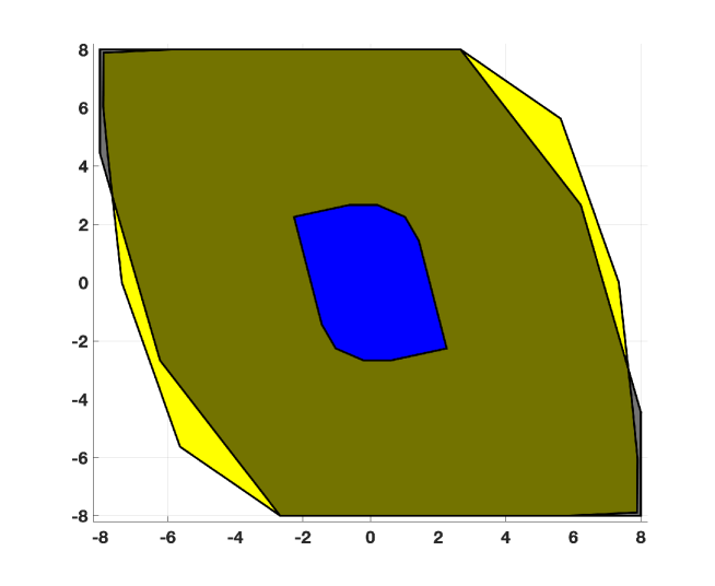
Figure 1: Comparison of the Approximate Region of Attraction of Algorithm 1 and the convex hull of the feasible initial state samples with tube MPC in [21, Section 5] and constrained LQR in [13, Section 2.3].

Recall the notion of the ROA of Algorithm 1 from Section 5 and also its inner approximation obtained from Algorithm 2. We now choose a set of $N_{\mathrm{init}}=100$ initial states $x_{S}$, created by a $10\times 10$ uniformly spaced grid of the set of state constraints in (29). From each of these initial state samples we check the feasibility of the tube MPC control problem in [21, Section 5]. The source code to solve the tube MPC is adapted from [10]. The convex hull of the feasible initial state samples, which inner approximates its ROA, is then compared to the approximate ROA of Algorithm 1. This comparison is shown in Fig. 1. The approximate ROA of Algorithm 1 is about 1.04x in volume of that of the tube MPC in [21, Section 5]. The advantage of our approach becomes clearer in Table 1.

Table 1: Average computation times [sec] comparison. Values are obtained with a MacBook Pro 16inch, 2019, 2.3 GHz 8-Core Intel Core i9, 16 GB memory, using the Gurobi solver [17].

Horizon	Algorithm 1		Tube MPC in [21]
	online	offline	online
$N_{t}=1$	0.0019	0	0.0054
$N_{t}=2$	0.0058	0.0279	0.1042
$N_{t}=3$	0.0111	0.0687	0.2057

We see from Table 1 that for all relevant horizon lengths $N_{t}\in\{1,2,3\}$, solving (24) is cheaper than computing the tube MPC online, even after adding the offline computation times required for bounds (35)-(39).

Remark 3.

Tube MPC methods such as [21, 26, 27, 15] also require offline matrix/set computations before online control design. See [19, Chapter 5] for further details. In the considered example, computing the set $Z$ for the tube MPC in [21] required about 49 seconds offline. However, we have chosen not to include this in the comparison in Table 1, as any alternative simpler choice of $Z$ is also valid. The choice of $Z$ affects the ROA [11].

6.2 Comparison with Constrained LQR [13]

Using the same 100 initial state samples, we now check the feasibility of the constrained LQR synthesis problem in [13, Section 2.3]. We run all the simulations for an FIR length (same as control horizon length) of $L=15$. The values of parameters for constraint tightenings are chosen as $\tau=0.99$ and $\tau_{\infty}=0.2$ after a grid search. See [13, Problem 2.8] for further details on these parameters. The convex hull of the feasible initial state samples with the algorithm of [13, Section 2.3], which inner approximates its ROA, is about $12$ times smaller in volume and is a subset of the approximate ROA of Algorithm 1, as seen in Fig. 1. Furthermore, as [13] does not solve any optimization problem for control synthesis for $t\geq 1$, we highlight that this gain in ROA volume can also be obtained with an open-loop policy given by:

$$\Pi^{\mathrm{safe}}_{\mathrm{ol}}(x_{t})=\begin{cases}u^{\star}_{t|0}(x_{t}),&\mbox{if }t\leq({N}-1),\\ Kx_{t},&\textnormal{otherwise}.\end{cases}$$ (30)

System (1) with (30) maintains robust satisfaction of (5e) for all time steps, without re-solving (24) after $t=0$. Moreover, the one-time control computation times with [13] are comparable. We omit showing these values due to the difference in programming languages.

7 Conclusions

We proposed a novel approach to design a robust Model Predictive Controller (MPC) for constrained uncertain linear systems. The uncertainty considered included both mismatch in the system dynamics matrices, and additive disturbance. The proposed MPC achieved robust satisfaction of the imposed state and input constraints for all realizations of the model uncertainty. We further proved Input to State Stability of the origin. With numerical simulations, we demonstrated that our controller obtained at least 3x and up to 20x speedup in online control computations and an approximately $4\%$ larger ROA by volume, compared to the tube MPC in [21]. We also demonstrated an approximately 12x decrease in conservatism over the constrained LQR algorithm of [13] using a safe open-loop policy.

Appendix A Appendix

A.1 Matrix Definitions

The prediction dynamics matrices $\mathbf{A}^{x},\mathbf{A}^{u},\mathbf{A}^{\Delta u}$ and $\mathbf{A}^{w}$ in (9) for a horizon length of $\bar{N}$ are given by

$$\mathbf{A}^{x} =\begin{bmatrix}A_{\Delta}&0&0&\dots&0\\ A_{\Delta}\Delta_{A}&A_{\Delta}&0&\dots&0\\ A_{\Delta}^{2}\Delta_{A}&A_{\Delta}\Delta_{A}&A_{\Delta}&\dots&0\\ \vdots&\vdots&\vdots&\ddots&\vdots\\ A_{\Delta}^{\bar{N}-1}\Delta_{A}&A_{\Delta}^{\bar{N}-2}\Delta_{A}&\dots&\dots&A_{\Delta}\end{bmatrix}\in\mathbb{R}^{d\bar{N}\times d\bar{N}},$$

$$\mathbf{A}^{u} =\begin{bmatrix}B_{\Delta}&0&0&\dots&0\\ A_{\Delta}\Delta_{B}&B_{\Delta}&0&\dots&0\\ A_{\Delta}^{2}\Delta_{B}&A_{\Delta}\Delta_{B}&B_{\Delta}&\dots&0\\ \vdots&\vdots&\vdots&\ddots&\vdots\\ A_{\Delta}^{\bar{N}-1}\Delta_{B}&A_{\Delta}^{\bar{N}-2}\Delta_{B}&\dots&\dots&B_{\Delta}\end{bmatrix}\in\mathbb{R}^{d\bar{N}\times m\bar{N}},$$

$$\mathbf{A}^{\Delta u} =\begin{bmatrix}0&0&0&\dots&0\\ A_{\Delta}\bar{B}&0&0&\dots&0\\ A_{\Delta}^{2}\bar{B}&A_{\Delta}\bar{B}&0&\dots&0\\ \vdots&\vdots&\vdots&\ddots&\vdots\\ A_{\Delta}^{\bar{N}-1}\bar{B}&A_{\Delta}^{\bar{N}-2}\bar{B}&\dots&A_{\Delta}\bar{B}&0\end{bmatrix}\in\mathbb{R}^{d\bar{N}\times m\bar{N}},$$

$$\mathbf{A}^{w} =\begin{bmatrix}I_{d}&0&0&\dots&0\\ A_{\Delta}&I_{d}&0&\dots&0\\ A_{\Delta}^{2}&A_{\Delta}&I_{d}&\dots&0\\ \vdots&\vdots&\vdots&\ddots&\vdots\\ A_{\Delta}^{\bar{N}-1}&A_{\Delta}^{\bar{N}-2}&\dots&\dots&I_{d}\end{bmatrix}\in\mathbb{R}^{d\bar{N}\times d\bar{N}},$$

where $A_{\Delta}=(\bar{A}+\Delta_{A})\in\mathcal{P}_{A_{\Delta}}$ and $B_{\Delta}=(\bar{B}+\Delta_{B})\in\mathcal{P}_{B_{\Delta}}$. We write matrices $\bar{\mathbf{A}}_{1}$ and $\mathbf{A}_{\delta}\in\mathbb{R}^{d\bar{N}\times d\bar{N}}$ as:

$$\bar{\mathbf{A}}_{1}=\begin{bmatrix}I_{d}&0&0&\dots&0\\ \bar{A}&I_{d}&0&\dots&0\\ \bar{A}^{2}&\bar{A}&I_{d}&\dots&0\\ \vdots&\vdots&\vdots&\ddots&\vdots\\ \bar{A}^{\bar{N}-1}&\bar{A}^{\bar{N}-2}&\dots&\dots&I_{d}\end{bmatrix},\leavevmode\nobreak\ \mathbf{A}_{\delta}=(\mathbf{A}^{w}-\bar{\mathbf{A}}_{1}),$$

which gives $\mathbf{A}^{x}=\bar{\mathbf{A}}+\Big{(}\bar{\mathbf{A}}_{1}+\mathbf{A}_{\delta}\Big{)}\mathbf{\Delta}_{A},\mathbf{A}^{u}=\bar{\mathbf{B}}+\Big{(}\bar{\mathbf{A}}_{1}+\mathbf{A}_{\delta}\Big{)}\mathbf{\Delta}_{B}$, and $\mathbf{A}^{\Delta u}=\Big{(}\bar{\mathbf{A}}_{1}-\mathbf{I}_{d}+\mathbf{A}_{\delta}\Big{)}\bar{\mathbf{B}}$. The matrix $\bar{\mathbf{A}}_{v}$ is written as $\bar{\mathbf{A}}_{v}=\begin{bmatrix}A^{(1)}_{v}&A^{(2)}_{v}&\dots&A^{(\bar{N}-1)}_{v}\end{bmatrix}$, where matrices $\{A^{(1)}_{v},A^{(2)}_{v},\dots,A^{(\bar{N}-1)}_{v}\}$ are given as

$$A^{(1)}_{v}=\begin{bmatrix}0&0&0&\dots&0\\ I_{d}&0&0&\dots&0\\ 0&I_{d}&0&\dots&0\\ \vdots&\vdots&\vdots&\ddots&\vdots\\ 0&0&\dots&I_{d}&0\end{bmatrix},\leavevmode\nobreak\ A^{(2)}_{v}=\begin{bmatrix}0&0&0&\dots&0\\ 0&0&0&\dots&0\\ I_{d}&0&0&\dots&0\\ 0&I_{d}&0&\dots&0\\ \vdots&\vdots&\vdots&\ddots&\vdots\\ 0&0&I_{d}&\dots&0\end{bmatrix},\leavevmode\nobreak\ \textnormal{and analogously for}\leavevmode\nobreak\ A^{(3)}_{v},\dots,A^{(\bar{N}-1)}_{v}.$$

This gives $\mathbf{A}^{w}=\mathbf{I}_{d}+\bar{\mathbf{A}}_{v}\mathbf{A}_{\Delta}$, with $\mathbf{I}_{d}=(I_{\bar{N}}\otimes I_{d})$, and

$$\mathbf{A}_{\Delta}=\begin{bmatrix}I_{\bar{N}}\otimes A_{\Delta}\\ I_{\bar{N}}\otimes A_{\Delta}^{2}\\ \vdots\\ I_{\bar{N}}\otimes A_{\Delta}^{\bar{N}-1}\end{bmatrix}\in\mathbb{R}^{d\bar{N}(\bar{N}-1)\times d\bar{N}}.$$ (31)

A.2 Deriving (3.2) from (12)

Using (11) in (9), constraints (12) can be written as:

$$\mathbf{F}^{x}\Bigg{(}\bar{\mathbf{A}}\bar{\mathbf{x}}_{t}+\bar{\mathbf{A}}_{1}\mathbf{\Delta}_{A}\bar{\mathbf{x}}_{t}+(\mathbf{A}_{\delta}\mathbf{\Delta}_{A})\bar{\mathbf{x}}_{t}+\bar{\mathbf{B}}\mathbf{u}_{t}+\bar{\mathbf{A}}_{1}\mathbf{\Delta}_{B}\mathbf{u}_{t}+(\mathbf{A}_{\delta}\mathbf{\Delta}_{B})\mathbf{u}_{t}+(\bar{\mathbf{A}}_{1}-\mathbf{I}_{d}+\mathbf{A}_{\delta})\bar{\mathbf{B}}\Delta\mathbf{u}_{t}+\cdots$$

$$\leavevmode\nobreak\ \leavevmode\nobreak\ \leavevmode\nobreak\ \leavevmode\nobreak\ \leavevmode\nobreak\ \leavevmode\nobreak\ \leavevmode\nobreak\ \leavevmode\nobreak\ \leavevmode\nobreak\ \leavevmode\nobreak\ \leavevmode\nobreak\ \leavevmode\nobreak\ \leavevmode\nobreak\ \leavevmode\nobreak\ \leavevmode\nobreak\ \leavevmode\nobreak\ \leavevmode\nobreak\ \leavevmode\nobreak\ \leavevmode\nobreak\ \leavevmode\nobreak\ \leavevmode\nobreak\ \leavevmode\nobreak\ \leavevmode\nobreak\ \leavevmode\nobreak\ \leavevmode\nobreak\ \leavevmode\nobreak\ \leavevmode\nobreak\ \leavevmode\nobreak\ \leavevmode\nobreak\ \leavevmode\nobreak\ \leavevmode\nobreak\ \leavevmode\nobreak\ \leavevmode\nobreak\ \leavevmode\nobreak\ \leavevmode\nobreak\ \leavevmode\nobreak\ \leavevmode\nobreak\ \leavevmode\nobreak\ \leavevmode\nobreak\ \leavevmode\nobreak\ \leavevmode\nobreak\ \leavevmode\nobreak\ \leavevmode\nobreak\ \leavevmode\nobreak\ \leavevmode\nobreak\ \leavevmode\nobreak\ \leavevmode\nobreak\ \leavevmode\nobreak\ \leavevmode\nobreak\ \leavevmode\nobreak\ \leavevmode\nobreak\ \leavevmode\nobreak\ \leavevmode\nobreak\ \leavevmode\nobreak\ \leavevmode\nobreak\ \leavevmode\nobreak\ \leavevmode\nobreak\ \leavevmode\nobreak\ \leavevmode\nobreak\ \leavevmode\nobreak\ \leavevmode\nobreak\ \leavevmode\nobreak\ \leavevmode\nobreak\ \leavevmode\nobreak\ \leavevmode\nobreak\ \leavevmode\nobreak\ \leavevmode\nobreak\ \leavevmode\nobreak\ \leavevmode\nobreak\ \leavevmode\nobreak\ \leavevmode\nobreak\ \leavevmode\nobreak\ \leavevmode\nobreak\ \leavevmode\nobreak\ \leavevmode\nobreak\ \leavevmode\nobreak\ \leavevmode\nobreak\ \leavevmode\nobreak\ \leavevmode\nobreak\ \leavevmode\nobreak\ \leavevmode\nobreak\ \leavevmode\nobreak\ \leavevmode\nobreak\ \leavevmode\nobreak\ \leavevmode\nobreak\ \leavevmode\nobreak\ +\mathbf{w}_{t}+\bar{\mathbf{A}}_{v}\mathbf{A}_{\Delta}\mathbf{w}_{t}\Bigg{)}\leq\mathbf{f}^{x},$$ (32)

$$\forall\Delta_{A}\in\mathcal{P}_{A},\leavevmode\nobreak\ \forall\Delta_{B}\in\mathcal{P}_{B},\leavevmode\nobreak\ \forall w_{t}\in\mathbb{W}.$$

We obtain an upper bound for the left hand side of inequality (A.2) row-wise as follows:

$$\mathbf{F}^{x}_{i}(\bar{\mathbf{A}}\bar{\mathbf{x}}_{t}+\bar{\mathbf{B}}\mathbf{u}_{t}+(\bar{\mathbf{A}}_{1}-\mathbf{I}_{d})\bar{\mathbf{B}}\Delta\mathbf{u}_{t}+\mathbf{w}_{t})+\mathbf{F}^{x}_{i}\bar{\mathbf{A}}_{1}\mathbf{\Delta}_{A}\bar{\mathbf{x}}_{t}+\mathbf{F}^{x}_{i}\bar{\mathbf{A}}_{1}\mathbf{\Delta}_{B}\mathbf{u}_{t}+\mathbf{F}^{x}_{i}\mathbf{A}_{\delta}\mathbf{\Delta}_{A}\bar{\mathbf{x}}_{t}+\cdots$$

$$\leavevmode\nobreak\ \leavevmode\nobreak\ \leavevmode\nobreak\ \leavevmode\nobreak\ \leavevmode\nobreak\ \leavevmode\nobreak\ \leavevmode\nobreak\ \leavevmode\nobreak\ \leavevmode\nobreak\ \leavevmode\nobreak\ \leavevmode\nobreak\ \leavevmode\nobreak\ \leavevmode\nobreak\ \leavevmode\nobreak\ \leavevmode\nobreak\ \leavevmode\nobreak\ \leavevmode\nobreak\ \leavevmode\nobreak\ \leavevmode\nobreak\ \leavevmode\nobreak\ \leavevmode\nobreak\ \leavevmode\nobreak\ \leavevmode\nobreak\ \leavevmode\nobreak\ \leavevmode\nobreak\ \leavevmode\nobreak\ \leavevmode\nobreak\ \leavevmode\nobreak\ \leavevmode\nobreak\ \leavevmode\nobreak\ \leavevmode\nobreak\ \leavevmode\nobreak\ \leavevmode\nobreak\ \leavevmode\nobreak\ \leavevmode\nobreak\ \leavevmode\nobreak\ \leavevmode\nobreak\ \leavevmode\nobreak\ \leavevmode\nobreak\ \leavevmode\nobreak\ \leavevmode\nobreak\ \leavevmode\nobreak\ \leavevmode\nobreak\ \leavevmode\nobreak\ \leavevmode\nobreak\ \leavevmode\nobreak\ \leavevmode\nobreak\ \leavevmode\nobreak\ \leavevmode\nobreak\ \leavevmode\nobreak\ \leavevmode\nobreak\ +\mathbf{F}^{x}_{i}\mathbf{A}_{\delta}\mathbf{\Delta}_{B}\mathbf{u}_{t}+\mathbf{F}^{x}_{i}\mathbf{A}_{\delta}\bar{\mathbf{B}}\Delta\mathbf{u}_{t}+\mathbf{F}^{x}_{i}\bar{\mathbf{A}}_{v}\mathbf{A}_{\Delta}\mathbf{w}_{t},$$

$$\leq\mathbf{F}^{x}_{i}(\bar{\mathbf{A}}\bar{\mathbf{x}}_{t}+\bar{\mathbf{B}}\mathbf{u}_{t}+(\bar{\mathbf{A}}_{1}-\mathbf{I}_{d})\bar{\mathbf{B}}\Delta\mathbf{u}_{t}+\mathbf{w}_{t})+\mathbf{F}^{x}_{i}\bar{\mathbf{A}}_{1}\mathbf{\Delta}_{A}\bar{\mathbf{x}}_{t}+\mathbf{F}^{x}_{i}\bar{\mathbf{A}}_{1}\mathbf{\Delta}_{B}\mathbf{u}_{t}+\|\mathbf{F}^{x}_{i}\mathbf{A}_{\delta}\mathbf{\Delta}_{A}\|_{*}\|\bar{\mathbf{x}}_{t}\|+$$

$$\leavevmode\nobreak\ \leavevmode\nobreak\ \leavevmode\nobreak\ \leavevmode\nobreak\ \leavevmode\nobreak\ \leavevmode\nobreak\ \leavevmode\nobreak\ \leavevmode\nobreak\ \leavevmode\nobreak\ \leavevmode\nobreak\ \leavevmode\nobreak\ \leavevmode\nobreak\ \leavevmode\nobreak\ \leavevmode\nobreak\ \leavevmode\nobreak\ \leavevmode\nobreak\ \leavevmode\nobreak\ \leavevmode\nobreak\ \leavevmode\nobreak\ \leavevmode\nobreak\ \leavevmode\nobreak\ \leavevmode\nobreak\ \leavevmode\nobreak\ \leavevmode\nobreak\ \leavevmode\nobreak\ \leavevmode\nobreak\ \leavevmode\nobreak\ \leavevmode\nobreak\ \leavevmode\nobreak\ \leavevmode\nobreak\ \leavevmode\nobreak\ \leavevmode\nobreak\ \leavevmode\nobreak\ \leavevmode\nobreak\ \leavevmode\nobreak\ \leavevmode\nobreak\ \cdots+\|\mathbf{F}^{x}_{i}\mathbf{A}_{\delta}\mathbf{\Delta}_{B}\|_{*}\|\mathbf{u}_{t}\|+\|\mathbf{F}^{x}_{i}\mathbf{A}_{\delta}\bar{\mathbf{B}}\|_{*}\|\Delta\mathbf{u}_{t}\|+\|\mathbf{F}^{x}_{i}\bar{\mathbf{A}}_{v}\mathbf{A}_{\Delta}\|_{*}\|\mathbf{w}_{t}\|,$$ (33)

for rows $i\in\{1,2,\dots,r(\bar{N}-1)+r_{N}\}$, where we have used the Hölder’s inequality. Using bounds (35)-(39) in (A.2) then yields (3.2). Note that in (3.2) $\bar{N}\leftarrow N$.

A.3 Bounding Nominal Trajectory Perturbations

For any horizon length of $\bar{N}\in\{2,3,\dots,N\}$, we first bound:

$$\max_{A_{\Delta}\in\mathcal{P}_{A_{\Delta}}}\|\mathbf{F}^{x}_{i}\mathbf{A}_{\delta}\|_{*},\leavevmode\nobreak\ \textnormal{where using \eqref{padelta} we have}$$

$$\mathbf{A}_{\delta}=\bar{\mathbf{A}}_{v}\begin{bmatrix}I_{\bar{N}}\otimes(A_{\Delta}-\bar{A})\\ I_{\bar{N}}\otimes(A_{\Delta}^{2}-\bar{A}^{2})\\ \vdots\\ I_{\bar{N}}\otimes(A_{\Delta}^{\bar{N}-1}-\bar{A}^{\bar{N}-1})\end{bmatrix}.$$ (34)

Note that for all $A_{\Delta}\in\mathcal{P}_{A_{\Delta}}\implies A_{\Delta}^{n}\in\mathcal{P}^{n}_{A_{\Delta}}$, for $n\in\{1,2,\dots,\bar{N}-1\}$, where $\mathcal{P}^{n}_{A_{\Delta}}$ is the set of all matrices that can be written as a convex combination of matrices obtained with the product of all possible combinations of $n$ matrices out of $\{(\bar{A}+\Delta^{(1)}_{A}),(\bar{A}+\Delta^{(2)}_{A}),\dots,(\bar{A}+\Delta^{(n_{a})}_{A})\}$. Hence

$$\max_{A_{\Delta}\in\mathcal{P}_{A_{\Delta}}}\|\mathbf{F}^{x}_{i}\mathbf{A}_{\delta}\|_{*}\leq\max_{\begin{subarray}{c}\Delta_{1}\in\mathcal{P}_{A_{\Delta}}\\ \Delta_{2}\in\mathcal{P}^{2}_{A_{\Delta}}\\ \vdots\\ \Delta_{\bar{N}-1}\in\mathcal{P}^{\bar{N}-1}_{A_{\Delta}}\end{subarray}}\|\mathbf{F}^{x}_{i}\bar{\mathbf{A}}_{v}\begin{bmatrix}I_{N}\otimes(\Delta_{1}-\bar{A})\\ I_{N}\otimes(\Delta_{2}-\bar{A}^{2})\\ \vdots\\ I_{N}\otimes(\Delta_{\bar{N}-1}-\bar{A}^{\bar{N}-1})\end{bmatrix}\|_{*}=\mathbf{t}^{i}_{0},$$ (35)

where we have relaxed all the equality constraints among the matrices $\{\Delta_{1},\Delta_{2},\dots,\Delta_{\bar{N}-1}\}$. Using the above bound (35), we get

$$\max_{\begin{subarray}{c}A_{\Delta}\in\mathcal{P}_{A_{\Delta}}\\ \Delta_{A}\in\mathcal{P}_{A}\end{subarray}}\|\mathbf{F}^{x}_{i}\mathbf{A}_{\delta}\mathbf{\Delta}_{A}\|_{*}\leq\mathbf{t}^{i}_{0}\max_{\Delta_{A}\in\mathcal{P}_{A}}\|\mathbf{\Delta}_{A}\|_{p}=\mathbf{t}^{i}_{1},$$ (36)

where we have used the consistency property of induced norms, for any $p=1,2,\infty$. Similarly, bounding terms

$$\max_{\begin{subarray}{c}A_{\Delta}\in\mathcal{P}_{A_{\Delta}}\\ \Delta_{B}\in\mathcal{P}_{B}\end{subarray}}\|\mathbf{F}^{x}_{i}\mathbf{A}_{\delta}\mathbf{\Delta}_{B}\|_{*}\leq\mathbf{t}^{i}_{0}\max_{\Delta_{B}\in\mathcal{P}_{B}}\|\mathbf{\Delta}_{B}\|_{p}=\mathbf{t}^{i}_{2},$$ (37)

and

$$\max_{A_{\Delta}\in\mathcal{P}_{A_{\Delta}}}\|\mathbf{F}^{x}_{i}\mathbf{A}_{\delta}\bar{\mathbf{B}}\|_{*}\leq\mathbf{t}^{i}_{0}\|\bar{\mathbf{B}}\|_{p}=\mathbf{t}^{i}_{3},$$ (38)

and finally

$$\max_{A_{\Delta}\in\mathcal{P}_{A_{\Delta}}}\|\mathbf{F}^{x}_{i}\bar{\mathbf{A}}_{v}\mathbf{A}_{\Delta}\|_{*}\leq\max_{\begin{subarray}{c}\Delta_{1}\in\mathcal{P}_{A_{\Delta}}\\ \Delta_{2}\in\mathcal{P}^{2}_{A_{\Delta}}\\ \vdots\\ \Delta_{\bar{N}-1}\in\mathcal{P}^{\bar{N}-1}_{A_{\Delta}}\end{subarray}}\|\mathbf{F}^{x}_{i}\bar{\mathbf{A}}_{v}\begin{bmatrix}I_{\bar{N}}\otimes\Delta_{1}\\ I_{\bar{N}}\otimes\Delta_{2}\\ \vdots\\ I_{\bar{N}}\otimes\Delta_{\bar{N}-1}\end{bmatrix}\|_{*}=\mathbf{t}^{i}_{w},$$ (39)

for $i\in\{1,2,\dots,r(\bar{N}-1)+r_{N}\}$. Problems (35)-(39) are maximizing convex functions of the decision variables over convex and compact domains. Therefore, these maximum bounds are attained at the extreme points, i.e., vertices of the convex sets $\{\mathcal{P}_{A_{\Delta}},\mathcal{P}^{2}_{A_{\Delta}},\dots,\mathcal{P}^{\bar{N}-1}_{A_{\Delta}}\}$, $\mathcal{P}_{A}$ and $\mathcal{P}_{B}$. Consequently, the optimal values of (35)-(39) can be obtained by evaluating the values of each of the terms in (35)-(39) at all possible combinations of such extreme points. Since such a vertex enumeration strategy scales poorly with the horizon length $N$, a computationally cheaper alternative to bounds (35)-(39) is presented next.

A.4 Computationally Efficient Alternatives of Bounds (35)-(39)

Recall the optimization problem from (35), given by

$$\max_{A_{\Delta}\in\mathcal{P}_{A_{\Delta}}}\|\mathbf{F}^{x}_{i}\mathbf{A}_{\delta}\|_{*},\leavevmode\nobreak\ \textnormal{with $\mathbf{A}_{\delta}$ from \eqref{adlta}}.$$ (40)

Using the triangle and Hölder’s inequalities, and the submultiplicativity and consistency properties of induced norms, (40) can be upper bounded for any cut-off horizon $\tilde{N}<\bar{N}$ as follows:

$$\max_{A_{\Delta}\in\mathcal{P}_{A_{\Delta}}}\|\mathbf{F}^{x}_{i}\mathbf{A}_{\delta}\|_{*}\leq\tilde{\mathbf{t}}^{i}_{0}+\hat{\mathbf{t}}^{i}_{0}=\mathbf{t}^{i}_{0},$$ (41)

with

$$\tilde{\mathbf{t}}^{i}_{0}=\max_{\begin{subarray}{c}\Delta_{1}\in\mathcal{P}_{A_{\Delta}}\\ \vdots\\ \Delta_{\tilde{N}-1}\in\mathcal{P}^{\tilde{N}-1}_{A_{\Delta}}\end{subarray}}\|\mathbf{F}^{x}_{i}\bar{\mathbf{A}}^{1:(\tilde{N}-1)}_{v}\begin{bmatrix}I_{\bar{N}}\otimes(\Delta_{1}-\bar{A})\\ I_{\bar{N}}\otimes(\Delta_{2}-\bar{A}^{2})\\ \vdots\\ I_{\bar{N}}\otimes(\Delta_{\tilde{N}-1}-\bar{A}^{\tilde{N}-1})\end{bmatrix}\|_{*}$$

where $\bar{\mathbf{A}}^{n_{1}:n_{2}}_{v}$ denotes $\begin{bmatrix}A^{(n_{1})}_{v}&A^{(n_{1}+1)}_{v}&\dots&A^{(n_{2})}_{v}\end{bmatrix}$, with the associated matrices defined in Appendix A.1, $\mathbf{F}_{i}^{x}[n_{1}:n_{2}]$ denotes the $n_{1}$ to $n_{2}$ columns of the row vector $\mathbf{F}^{x}_{i}$, for $i\in\{1,2,\dots,r(\bar{N}-1)+r_{N}\}$, and

$$\hat{\mathbf{t}}^{i}_{0}=\max_{\Delta_{A}\in\mathcal{P}_{A}}\Bigg{(}\sum_{j=\tilde{N}+1}^{\bar{N}}\|\mathbf{F}^{x}_{i}[(j-1)d+1:jd]\|_{*}\big{(}\sum_{k=1}^{j-\tilde{N}}(\sum_{l=1}^{j-k}{j-k\choose l}\|\bar{A}\|^{j-k-l}_{p}\|\Delta_{A}\|^{l}_{p})\big{)}\Bigg{)}.$$

Using the above derived bound (41) we obtain:

$$\max_{\begin{subarray}{c}A_{\Delta}\in\mathcal{P}_{A_{\Delta}}\\ \Delta_{A}\in\mathcal{P}_{A}\end{subarray}}\|\mathbf{F}^{x}_{i}\mathbf{A}_{\delta}\mathbf{\Delta}_{A}\|_{*}\leq\mathbf{t}^{i}_{0}\max_{\Delta_{A}\in\mathcal{P}_{A}}\|\mathbf{\Delta}_{A}\|_{p}=\mathbf{t}^{i}_{1},$$

where we have used the consistency property of induced norms, for any $p=1,2,\infty$. Similarly, we bound

$$\max_{\begin{subarray}{c}A_{\Delta}\in\mathcal{P}_{A_{\Delta}}\\ \Delta_{B}\in\mathcal{P}_{B}\end{subarray}}\|\mathbf{F}^{x}_{i}\mathbf{A}_{\delta}\mathbf{\Delta}_{B}\|_{*}\leq\mathbf{t}^{i}_{0}\max_{\Delta_{B}\in\mathcal{P}_{B}}\|\mathbf{\Delta}_{B}\|_{p}=\mathbf{t}^{i}_{2},$$

and,

$$\max_{A_{\Delta}\in\mathcal{P}_{A_{\Delta}}}\|\mathbf{F}^{x}_{i}{\mathbf{A}}_{\delta}\bar{\mathbf{B}}\|_{*}\leq\mathbf{t}^{i}_{0}\|\bar{\mathbf{B}}\|_{p}=\mathbf{t}^{i}_{3},$$

and finally using $\mathbf{A}_{\Delta}$ from (31)

$$\max_{A_{\Delta}\in\mathcal{P}_{A_{\Delta}}}\|\mathbf{F}^{x}_{i}\bar{\mathbf{A}}_{v}\mathbf{A}_{\Delta}\|_{*}\leq\tilde{\mathbf{t}}^{i}_{w}+\hat{\mathbf{t}}^{i}_{w}={\mathbf{t}}^{i}_{w},$$

for all $i\in\{1,2,\dots,r(\bar{N}-1)+r_{N}\}$, where

$$\tilde{\mathbf{t}}^{i}_{w}=\max_{\begin{subarray}{c}\Delta_{1}\in\mathcal{P}_{A_{\Delta}}\\ \vdots\\ \Delta_{\tilde{N}-1}\in\mathcal{P}^{\tilde{N}-1}_{A_{\Delta}}\end{subarray}}\|\mathbf{F}^{x}_{i}\bar{\mathbf{A}}^{1:(\tilde{N}-1)}_{v}\begin{bmatrix}I_{\bar{N}}\otimes\Delta_{1}\\ I_{\bar{N}}\otimes\Delta_{2}\\ \vdots\\ I_{\bar{N}}\otimes\Delta_{\tilde{N}-1}\end{bmatrix}\|_{*},$$

and

$$\hat{\mathbf{t}}^{i}_{w}=\max_{\Delta_{A}\in\mathcal{P}_{A}}\Bigg{(}\sum_{j=\tilde{N}}^{\bar{N}-1}\|\mathbf{F}^{x}_{i}A^{(j)}_{v}\|_{*}\Big{(}\|(I_{\bar{N}}\otimes\bar{A})^{j}\|_{p}+\sum_{k=1}^{j}{j\choose k}\|(I_{\bar{N}}\otimes\bar{A})\|^{j-k}_{p}\|(I_{\bar{N}}\otimes\Delta_{A})\|^{k}_{p}\Big{)}\Bigg{)},$$

where we have used the property of two matrices $X$ and $Y$ yielding:

$$\|(X+Y)^{n}\|_{p}\leq\|X^{n}\|_{p}+\sum_{k=1}^{n}{n\choose k}\|X\|_{p}^{n-k}\|Y\|_{p}^{k},$$

$$\forall n\in\{\tilde{N},\tilde{N}+1,\dots,\bar{N}-1\}.$$

This cut-off horizon $\tilde{N}$ can be chosen based on the available computational resources at the expense of more conservatism over (35)-(39).

A.5 Obtaining (19) from (3.2)

Here we derive (19) from (3.2). Using bounds (21) and (35)-(39) and policy parametrization (14), constraints (3.2) can be satisfied by imposing:

$$\max_{\mathbf{w}_{t}\in\mathbf{W}}\Bigg{(}\mathbf{F}^{x}_{i}(\bar{\mathbf{A}}\bar{\mathbf{x}}^{(N_{t})}_{t}+\bar{\mathbf{B}}(\mathbf{M}^{(N_{t})}_{t}\mathbf{w}_{t}+\bar{\mathbf{u}}^{(N_{t})}_{t})+(\bar{\mathbf{A}}_{1}-\mathbf{I}_{d})\bar{\mathbf{B}}\mathbf{M}^{(N_{t})}_{t}\mathbf{w}_{t}+\mathbf{w}_{t})+\mathbf{t}_{\delta 1}^{(N_{t}),i}\|\bar{\mathbf{x}}_{t}^{(N_{t})}\|+\cdots$$

$$\leavevmode\nobreak\ \leavevmode\nobreak\ \leavevmode\nobreak\ \leavevmode\nobreak\ \leavevmode\nobreak\ \leavevmode\nobreak\ \leavevmode\nobreak\ \leavevmode\nobreak\ \leavevmode\nobreak\ \leavevmode\nobreak\ \leavevmode\nobreak\ \leavevmode\nobreak\ \leavevmode\nobreak\ +(\mathbf{t}_{2}^{(N_{t}),i}+\mathbf{t}_{\delta B}^{(N_{t}),i})\|\mathbf{M}^{(N_{t})}_{t}\mathbf{w}_{t}+\bar{\mathbf{u}}^{(N_{t})}_{t}\|+\mathbf{t}_{3}^{(N_{t}),i}\|\mathbf{M}^{(N_{t})}_{t}\mathbf{w}_{t}\|+\mathbf{t}_{w}^{(N_{t}),i}\mathbf{w}_{\mathrm{max}}\Bigg{)}\leq\mathbf{f}^{x}_{i},$$ (42)

where using (21) we have used the Hölder’s and the triangle inequality to bound $\mathbf{F}^{x}_{i}\bar{\mathbf{A}}_{1}\mathbf{\Delta}_{A}\bar{\mathbf{x}}^{(N_{t})}_{t}$ and $\mathbf{F}^{x}_{i}\bar{\mathbf{A}}_{1}\mathbf{\Delta}_{B}(\mathbf{M}^{(N_{t})}_{t}\mathbf{w}_{t}+\bar{\mathbf{u}}^{(N_{t})}_{t})$ for all rows $i\in\{1,2,\dots,r(N_{t}-1)+r_{N}\}$. Use the induced norm consistency property and the triangle inequality in (A.5) as:

$$(\mathbf{t}_{2}^{(N_{t}),i}+\mathbf{t}_{\delta B}^{(N_{t}),i})\|\mathbf{M}^{(N_{t})}_{t}\mathbf{w}_{t}+\bar{\mathbf{u}}^{(N_{t})}_{t}\|+\mathbf{t}^{(N_{t})}_{3}\|\mathbf{M}^{(N_{t})}_{t}\mathbf{w}_{t}\|,$$ (43)

$$\leq(\mathbf{t}_{2}^{(N_{t}),i}+\mathbf{t}_{\delta B}^{(N_{t}),i}+\mathbf{t}_{3}^{(N_{t}),i})\|\mathbf{M}^{(N_{t})}_{t}\|_{p}\mathbf{w}_{\mathrm{max}}+(\mathbf{t}_{2}^{(N_{t}),i}+\mathbf{t}_{\delta B}^{(N_{t}),i})\|\bar{\mathbf{u}}^{(N_{t})}_{t}\|,$$

$$\leq\mathbf{t}_{\delta 3}^{(N_{t}),i}\|\mathbf{M}^{(N_{t})}_{t}\|_{p}\mathbf{w}_{\mathrm{max}}+\mathbf{t}_{\delta 2}^{(N_{t}),i}\|\bar{\mathbf{u}}^{(N_{t})}_{t}\|,$$

for any $p=1,2,\infty$, where we have used the definitions (21). Using (43) in (A.5) for all rows $i\in\{1,2,\dots,r(N_{t}-1)+r_{N}\}$, we define

$$\!\mathbf{f}^{x}_{\mathrm{tight}} \!=\!\mathbf{f}^{x}\!-\!\mathbf{t}^{(N_{t})}_{\delta 1}\|\bar{\mathbf{x}}_{t}^{(N_{t})}\|\!-\!\mathbf{t}^{(N_{t})}_{\delta 3}\|\mathbf{M}^{(N_{t})}_{t}\|_{p}\mathbf{w}_{\mathrm{max}}-\mathbf{t}^{(N_{t})}_{\delta 2}\|\bar{\mathbf{u}}^{(N_{t})}_{t}\|-\mathbf{t}^{(N_{t})}_{w}\mathbf{w}_{\mathrm{max}},$$

which yields (19) with tightened constraints (20).

A.6 Reformulation of (24) via Duality of Convex Programs

We again consider the following two cases for satisfying the robust state constraints (19).
Case 1: ($N_{t}\geq 2$, i.e., $t\leq N-2$) Constraints (19a) can be satisfied using duality of convex programs by solving:

$$\mathbf{F}^{x}(\bar{\mathbf{A}}\bar{\mathbf{x}}^{(N_{t})}_{t}+\bar{\mathbf{B}}\bar{\mathbf{u}}^{(N_{t})}_{t})+\Lambda^{(N_{t})}\mathbf{h}^{w}\leq\mathbf{f}_{\mathrm{tight}}^{x},$$

$$\Lambda^{(N_{t})}\geq 0,$$

$$\Lambda^{(N_{t})}\mathbf{H}^{w}=\Big{(}\mathbf{F}^{x}(\bar{\mathbf{B}}\mathbf{M}^{(N_{t})}_{t}+(\bar{\mathbf{A}}_{1}-\mathbf{I}_{d})\bar{\mathbf{B}}\mathbf{M}^{(N_{t})}_{t}+\mathbf{I}_{d})\Big{)},$$

where $\mathbf{f}^{x}_{\mathrm{tight}}$ is obtained from (20), and dual variables $\Lambda^{(N_{t})}\in\mathbb{R}^{(r(N_{t}-1)+r_{N})\times aN_{t}}$.
Case 2: ($N_{t}=1$, i.e., $t\geq N-1$) Consider the case of $N_{t}=1$. As pointed out in (19b), the robust state constraint for this case can be simplified and written as

$$\max_{\begin{subarray}{c}{w}_{t}\in\mathbb{W}\\ \Delta_{A}\in\mathcal{P}_{A}\\ \Delta_{B}\in\mathcal{P}_{B}\end{subarray}}H^{x}_{N}((\bar{{A}}+{\Delta}_{A})\bar{\mathbf{x}}^{(1)}_{t}+(\bar{{B}}+{\Delta}_{B})\bar{\mathbf{u}}^{(1)}_{t}+{w}_{t})\leq h^{x}_{N},$$

which we must solve exactly (i.e., find $h^{x}_{N}$ where the max is attained) for the uncertainty representation ${w}_{t}\in\mathbb{W},\leavevmode\nobreak\ \Delta_{A}\in\mathcal{P}_{A}$ and $\Delta_{B}\in\mathcal{P}_{B}$, in order for guarantees of Theorem 1 to hold. Using duality of convex programs [5] one can write the robust state constraints (19b) equivalently as:

$$H^{x}_{N}((\bar{{A}}+\Delta^{(j)}_{A})\bar{\mathbf{x}}^{(1)}_{t}+(\bar{{B}}+\Delta^{(k)}_{B}){\bar{\mathbf{u}}}^{(1)}_{t})+\Lambda^{(1)}h^{w}\leq h^{x}_{N},$$

$$\Lambda^{(1)}\geq 0,\leavevmode\nobreak\ H^{x}_{N}=\Lambda^{(1)}H^{w},$$

$$\forall j\in\{1,2,\dots,n_{a}\},\leavevmode\nobreak\ \forall k\in\{1,2,\dots,n_{b}\},$$ (44)

where dual variables $\Lambda^{(1)}\in\mathbb{R}^{r_{N}\times a}$.
Input Constraints: Considering the robust input constraints (23) for any $N_{t}\in\{1,2,\dots,N\}$, one can similarly show that this is equivalent to:

$$(\gamma^{(N_{t})})^{\top}\mathbf{h}^{w}\leq\mathbf{h}^{u}-\mathbf{H}^{u}\bar{\mathbf{u}}^{(N_{t})}_{t},$$

$$(\mathbf{H}^{u}\mathbf{M}^{(N_{t})}_{t})^{\top}=(\mathbf{H}^{w})^{\top}\gamma^{(N_{t})},\leavevmode\nobreak\ \gamma^{(N_{t})}\geq 0,$$

by introducing decision variables of $\gamma^{(N_{t})}\in\mathbb{R}^{aN_{t}\times oN_{t}}$ in (24) for each horizon length $N_{t}\in\{1,2,\dots,N\}$.

A.7 Proof of Theorem 1

By assumption, at time step $t=0$ problem (24) with tightened constraints (20) is feasible, with a horizon length $N_{t}=N$. We then prove robust satisfaction of (5e) at all time steps $t\geq 0$ with controller (25) in closed-loop, by considering the following two cases:
Case 1: ($2\leq N_{t}<N$, i.e., $0<t\leq N-2$) As (24) is feasible at time step $t=0$ for $N_{t}=N$ chosen as per (18), let the corresponding optimal policy sequence be

$$\{u^{\star}_{0|0},u^{\star}_{1|0}(\cdot),\dots,u^{\star}_{N-1|0}(\cdot)\}.$$ (45)

For time steps $t\in\{1,2,\dots,N-2\}$ recall that we define the MPC policy in (25) as:

$$u^{\mathrm{MPC}}_{t}(x_{t})=\begin{cases}\bar{u}^{\star}_{t|t},\leavevmode\nobreak\ \textnormal{if \eqref{eq:MPC_R_fin_trac} is feasible,}\\ u^{\star}_{t|t_{\mathrm{f}}}(x_{t}),\leavevmode\nobreak\ \textnormal{otherwise},\end{cases}$$ (46)

where $t_{\mathrm{f}}\in\{0,1,\dots,N-1\}$ is the latest time step when (24) was feasible. Policy (46) satisfies (5e) robustly for all $t\in\{1,2,\dots,N-2\}$, as it is a solution to the constrained robust optimal control problem (24). Moreover, from (45), we have that $t_{\mathrm{f}}=0$ is a guaranteed certificate, in case (24) continues to be infeasible for all $t\in\{1,2,\dots,N-2\}$.
Case 2: ($N_{t}=1$, i.e., $t\geq N-1$) Consider the time step $t=N-1$, where from (18) the MPC horizon length $N_{t}=1$. In this case we consider constraints (19b) given by:

$$\max_{\begin{subarray}{c}{w}_{t}\in\mathbb{W}\\ \Delta_{A}\in\mathcal{P}_{A}\\ \Delta_{B}\in\mathcal{P}_{B}\end{subarray}}H^{x}_{N}((\bar{{A}}+{\Delta}_{A})\bar{\mathbf{x}}^{(1)}_{t}+({\bar{B}}+{\Delta}_{B})\bar{\mathbf{u}}^{(1)}_{t}+{w}_{t})\leq h^{x}_{N}.$$ (47)

From (46) we know that at time step $t=N-1$, there exists a $t_{\mathrm{f}}$ such that control action $u^{\star}_{t|t_{\mathrm{f}}}(x_{t})$ robustly steers the state $x_{t}$ to $\mathcal{X}_{N}$ in one time step.

Now, at $t=N-1$, we solve (47) exactly (i.e., find $h^{x}_{N}$ where the max is attained) by using duality arguments in (A.6), without any uncertainty over-approximation. Therefore, the optimization problem (24) with constraint (47) is guaranteed to be feasible at $t=N-1$, with $u^{\star}_{N-1|t_{\mathrm{f}}}(\cdot)$ as a feasibility certificate. Let us denote the corresponding optimal policy from $t=N-1$ as:

$$u^{\mathrm{MPC}}_{t}(x_{t})=\bar{u}^{\star}_{t|t}.$$ (48)

Let policy (48) be applied to (1) in closed-loop, so that the system reaches the terminal set $\mathcal{X}_{N}$ at time step $t+1$. Consider solving (47) at this step with a horizon length of $N_{t+1}=1$. As, constraint (47) uses the same representation of the system uncertainty in satisfying (5e)-(5f) robustly as done in (17), we can infer that a candidate policy at time step $(t+1)$ is

$$u_{t+1|t+1}(x_{t+1})=Kx_{t+1},$$ (49)

which is a feasible solution to the robust optimization problem (24) under constraint (47). Thus, (24) is guaranteed to remain feasible at $(t+1)$ with $N_{t+1}=1$. This completes the proof. $\blacksquare$

A.8 Proof of Theorem 2

First, we have from Case-2 in the proof of Theorem 1 that at time step $t=N-1$, the problem (24) is feasible with horizon $N_{t}=1$ and therefore $x_{t}\in\mathcal{X}_{N}$ for all $t\geq N$.

Now, consider the case of $t\geq N$, i.e., $N_{t}=1$. Since (24) for $N_{t}=1$ can be reformulated into a parametric QP, $V_{t\rightarrow t+1}^{\mathrm{MPC}}(x_{t},0,1)$ is continuous and piecewise quadratic in $\mathcal{X}_{N}$ with $V_{t\rightarrow t+1}^{\mathrm{MPC}}(0,0,1)=0$ [4]. Hence, under Assumptions 3-4, using the standard proof of [16, Theorem 23], we conclude that the origin of closed-loop system (27) is ISS according to Definition 4, and $V^{\mathrm{MPC}}_{t\rightarrow t+1}(x_{t},0,1)$ is ISS Lyapunov function $\forall t\geq N$. $\blacksquare$

References

- [1] Carmen Amo Alonso and Nikolai Matni. Distributed and localized closed loop model predictive control via system level synthesis. In Conference on Decision and Control (CDC), pages 5598–5605. IEEE, 2020.
- [2] James Anderson, John C Doyle, Steven H Low, and Nikolai Matni. System level synthesis. Annual Reviews in Control, 2019.
- [3] Alberto Bemporad, Francesco Borrelli, and Manfred Morari. Min-max control of constrained uncertain discrete-time linear systems. IEEE Transactions on automatic control, 48(9):1600–1606, 2003.
- [4] Alberto Bemporad, Manfred Morari, Vivek Dua, and Efstratios N Pistikopoulos. The explicit LQR for constrained systems. Automatica, 38(1):3–20, 2002.
- [5] Aharon Ben-Tal, Laurent El Ghaoui, and Arkadi Nemirovski. Robust optimization, volume 28. Princeton University Press, 2009.
- [6] Franco Blanchini. Set invariance in control. Automatica, 35(11):1747–1767, 1999.
- [7] Francesco Borrelli, Alberto Bemporad, and Manfred Morari. Predictive control for linear and hybrid systems. Cambridge University Press, 2017.
- [8] Stephen Boyd, Laurent El Ghaoui, Eric Feron, and Venkataramanan Balakrishnan. Linear matrix inequalities in system and control theory, volume 15. Siam, 1994.
- [9] Marco C Campi and Erik Weyer. Finite sample properties of system identification methods. IEEE Transactions on Automatic Control, 47(8):1329–1334, 2002.
- [10] Shaoru Chen. Robust-MPC-SLS repository. URL https://github.com/unstable-zeros/robust-mpc-sls, 2020.
- [11] Shaoru Chen, Han Wang, Manfred Morari, Victor M Preciado, and Nikolai Matni. Robust closed-loop model predictive control via system level synthesis. In Conference on Decision and Control (CDC), pages 2152–2159. IEEE, 2020.
- [12] Luigi Chisci, J Anthony Rossiter, and Giovanni Zappa. Systems with persistent disturbances: predictive control with restricted constraints. Automatica, 37(7):1019–1028, 2001.
- [13] Sarah Dean, Stephen Tu, Nikolai Matni, and Benjamin Recht. Safely learning to control the constrained linear quadratic regulator. arXiv preprint arXiv:1809.10121, 2018.
- [14] Martin Evans, Mark Cannon, and Basil Kouvaritakis. Robust MPC for linear systems with bounded multiplicative uncertainty. In Conference on Decision and Control (CDC), pages 248–253. IEEE, 2012.
- [15] James Fleming, Basil Kouvaritakis, and Mark Cannon. Robust tube MPC for linear systems with multiplicative uncertainty. IEEE Transactions on Automatic Control, 60(4):1087–1092, 2014.
- [16] Paul J Goulart, Eric C Kerrigan, and Jan M Maciejowski. Optimization over state feedback policies for robust control with constraints. Automatica, 42(4):523–533, 2006.
- [17] Inc Gurobi Optimization. Gurobi optimizer reference manual. URL http://www. gurobi. com, 2015.
- [18] Mayuresh V Kothare, Venkataramanan Balakrishnan, and Manfred Morari. Robust constrained model predictive control using linear matrix inequalities. Automatica, 32(10):1361–1379, 1996.
- [19] Basil Kouvaritakis and Mark Cannon. Model predictive control: Classical, robust and stochastic. Springer, 2016.
- [20] Basil Kouvaritakis, J Anthony Rossiter, and Jan Schuurmans. Efficient robust predictive control. IEEE Transactions on automatic control, 45(8):1545–1549, 2000.
- [21] Wilbur Langson, Ioannis Chryssochoos, SV Raković, and David Q Mayne. Robust model predictive control using tubes. Automatica, 40(1):125–133, 2004.
- [22] YI Lee and B Kouvaritakis. Linear matrix inequalities and polyhedral invariant sets in constrained robust predictive control. International Journal of Robust and Nonlinear Control, 10(13):1079–1090, 2000.
- [23] Yuandan Lin, Eduardo Sontag, and Yuan Wang. Various results concerning set input-to-state stability. In Conference on Decision and Control (CDC), volume 2, pages 1330–1335. IEEE, 1995.
- [24] Johan Löfberg. Minimax approaches to robust model predictive control, volume 812. Linköping University Electronic Press, 2003.
- [25] David Q Mayne, James B Rawlings, Christopher V Rao, and Pierre OM Scokaert. Constrained model predictive control: Stability and optimality. Automatica, 36(6):789–814, 2000.
- [26] Diego Muñoz-Carpintero, Mark Cannon, and Basil Kouvaritakis. Recursively feasible robust MPC for linear systems with additive and multiplicative uncertainty using optimized polytopic dynamics. In Conference on Decision and Control (CDC), pages 1101–1106. IEEE, 2013.
- [27] Saša V Raković and Qifeng Cheng. Homothetic tube MPC for constrained linear difference inclusions. In Chinese Control and Decision Conference, pages 754–761. IEEE, 2013.
- [28] Saša V Raković, Basil Kouvaritakis, Mark Cannon, Christos Panos, and Rolf Findeisen. Parameterized tube model predictive control. IEEE Transactions on Automatic Control, 57(11):2746–2761, 2012.
- [29] Saša V Raković, Basil Kouvaritakis, Rolf Findeisen, and Mark Cannon. Homothetic tube model predictive control. Automatica, 48(8):1631–1638, 2012.
- [30] Saša V Raković, William S Levine, and Behçet Açikmese. Elastic tube model predictive control. In American Control Conference (ACC), pages 3594–3599. IEEE, 2016.
- [31] James Blake Rawlings and David Q Mayne. Model predictive control: Theory and design. Nob Hill Pub., 2009.
- [32] Ugo Rosolia, Xiaojing Zhang, and Francesco Borrelli. Robust learning model predictive control for linear systems performing iterative tasks. IEEE Transactions on Automatic Control, early access, 2021.
- [33] Pierre OM Scokaert and David Q Mayne. Min-max feedback model predictive control for constrained linear systems. IEEE Transactions on Automatic control, 43(8):1136–1142, 1998.
- [34] Bernardo A Hernandez Vicente and Paul A Trodden. Stabilizing predictive control with persistence of excitation for constrained linear systems. Systems & Control Letters, 126:58–66, 2019.
- [35] Rene Vidal, Shawn Schaffert, John Lygeros, and Shankar Sastry. Controlled invariance of discrete time systems. In in Hybrid Systems: Computation and Control. Citeseer, 1999.