Dynamic scale anomalous transport in QCD with electromagnetic background

Abstract

We discuss phenomenological implications of the anomalous transport induced by the scale anomaly in QCD coupled to an electromagnetic (EM) field, based on a dilaton effective theory. The scale anomalous current emerges in a way perfectly analogous to the conformal transport current induced in a curved spacetime background, or the Nernst current in Dirac and Weyl semimetals – both current forms are equivalent by a “Weyl transformation”. We focus on a spatially homogeneous system of QCD hadron phase, which is expected to be created after the QCD phase transition and thermalization. We find that the EM field can induce a dynamic oscillatory dilaton field which in turn induces the scale anomalous current. As the phenomenological applications, we evaluate the dilepton and diphoton productions induced from the dynamic scale anomalous current, and find that those productions include a characteristic peak structure related to the dynamic oscillatory dilaton, which could be tested in heavy ion collisions. We also briefly discuss the out-of-equilibrium particle production created by a nonadiabatic dilaton oscillation, which happens in a way of the so-called tachyonic preheating mechanism.

1 Introduction

The transport phenomena induced by chiral anomaly (dubbed chiral anomalous transports) have been extensively studied in heavy-ion collisions where both the strong electromagnetic (EM) fields (of the order of $m_{\pi}^{2}$ with $m_{\pi}$ pion mass) and the local parity odd domains with net chirality (due to, e.g., strong CP violating topological transition) are generated. The search of such chiral anomalous transports is one of the frontiers of current heavy-ion collision experiments and, if they are confirmed, it would significantly boost our understanding of the quantum chromodynamics (QCD) vacuum structure; see Refs.  Kharzeev:2015znc ; Hattori:2016emy ; Zhao:2019hta ; Liu:2020ymh for reviews.

Nowadays, the target field in which such chiral anomalous transports play some role has been extended with multiple aspects including not only QCD and condensed matter systems, but also applications to other cosmologically and theoretically important issues, such as production of the baryon number asymmetry of universe Joyce:1997uy ; Bamba:2006km ; Kamada:2016eeb ; Kamada:2016cnb ; Anber:2015yca ; Jimenez:2017cdr ; Domcke:2019mnd ; Domcke:2019qmm , inflationary scenarios with axion Turner:1987vd ; Garretson:1992vt ; Anber:2006xt , and a solution for the gauge-hierarchy problem Hook:2016mqo ; Choi:2016kke ; Tangarife:2017vnd ; Tangarife:2017rgl ; Fonseca:2018xzp . Thus, the anomalous transport physics has opened a vast ballpark in the theoretical particle physics.

Paying an attention to another candidate for possible emergence of anomalous transports in QCD, one may notice the scale symmetry. The scale symmetry of QCD is explicitly broken and anomalous due to quantum corrections, which is dictated even at the one-loop perturbative beta function in pure gluonic QCD (Yang-Mills). Coupled to quarks, the QCD scale current externally gets other anomalous parts from the quark mass terms, and electroweak gauge corrections which quarks perturbatively feel. Among them, in particular, the external EM fields should give a significant contribution to the induced anomalous-scale transport, with relevance enough to leave some phenomenological implications, in heavy ion collisions and/or early universe during the thermal history where strong EM fields exist as well. In this perspective, the anomalous transport from the scale anomaly (will be dubbed scale anomalous transport hereafter) might have provide an effect similar to the case with the chiral anomaly.

Such an EM-field-induced scale anomalous transport has recently been discussed in the contexts different from QCD Chernodub:2016lbo ; Chernodub:2017bbd ; Chernodub:2017jcp ; Zheng:2019xeu . The electric current $j_{\mu}$ has been proposed to emerge in quantum electrodynamics (QED) in a curved spacetime background :

$$\langle j^{\mu}(x)\rangle=-\frac{2\beta(e)}{e}F^{\mu\nu}(x)\partial_{\nu}\tau(x)+\frac{2\beta(e)}{e}\left(\partial_{\nu}F^{\nu\mu}(x)\right)\tau(x),$$ (1.1)

where $\tau(x)$ represents the scale factor of the curved spacetime metric, $g_{\mu\nu}=e^{2\tau(x)}\eta_{\mu\nu}$ with $\eta_{\mu\nu}$ being the flat spacetime metric, and $\beta(e)$ is the beta function of the EM coupling $e$. Phenomenological applications have also been discussed in condensed matter systems, such as Dirac and Weyl semimetals, that was called induced Nernst current Chernodub:2017jcp .

We note that although the current $j_{\mu}$ in Eq. (1.1) completely relies on the existence of the scale factor $\tau(x)$ of the curved background spacetime which vanishes in the flat spacetime, the same scale anomalous transport can actually happen also in flat spacetime, as we will derive in this paper based on low-energy effective theory of QCD. Furthermore, we will show that it would appear dynamically in low-energy QCD.

At low-energy regime, the physics of QCD can be described by the low-lying hadron spectra including pseudo Nambu-Goldstone bosons associated with the spontaneous breaking of the (approximate) chiral symmetry. The chiral manifold can in principle be extremely reduced to the one governed only by the lightest two flavors, up and down quarks, by integrating out the heavier hadrons, so that we have only isotriplet pions. Besides, an isosinglet scalar meson can couple to pions. This scalar meson can be isolated and singled out to be only the one, no matter how complicated mixing puzzle the isosinglet scalars can have, that may be identified as the $f_{0}(500)$ in the observed scalar meson spectroscopy.

Generically, such singlet scalar couplings including self-interactions should be parametric, not be under control. One possible way to model singlet scalars of this kind is to assume it to be a pseudo dilaton associated with the spontaneous breaking of the anomalous/approximate scale symmetry, which constrains the coupling form so as to satisfy the low-energy theorem of the anomalous/approximate scale symmetry breaking. In that case, the lightest isosinglet (or chiral singlet) scalar, being dilaton field, can (at least at the classical dynamics level) play a role of complete analogue to the scale factor in a curved background theory. Thus, in the QCD hadron dynamics the scale factor $\tau(x)$ in Eq.(1.1) should be rephrased as the dilaton background field, and hence, the scale anomalous transport necessarily shows up when coupled to the EM field as well.

In contrast to the scale factor in the spacetime metric which is considered as a background configuration, nontrivial features may come up: since the QCD dilaton is a dynamical particle in the low-energy QCD, the anomalous current should be dynamically generated having the close relation with the dilaton dynamics. Moreover, we may consider the environment of the early universe, where the hadron phase is expected to be created in a spatially (presumably almost) homogeneous form, after the QCD phase transition and thermalization of the hadron phase bubbles (even with feasible inhomogeneity by a supercooling) DeGrand:1984uq . The homogeneous hadron phase is thermalized with the temperature $\sim 100$ MeV DeGrand:1984uq ; Kim:2018byy ; Kim:2018knr , at which all hadrons already become nonrelativistic in the thermal bath with photon (but still strongly interacting each other in the kinetic equilibrium). Then the thermal loop corrections to the dilaton dynamics can safely be neglected (with all exponentially suppressed), so the external EM interactions would be most relevant to the dilaton, as well as the vacuum contributions by strong interactions with pions and dilatons themselves.

The situation in heavy-ion collisions may be different where the hadron phase is expected to be inhomogeneous. However, as a first approximation, we can take the homogeneous limit as a starting point and focus on the dynamical time evolution of the system; taking the inhomogeneity of the system into account would mask the dynamical features that we will explore and thus we leave it as a future task.

We emphasize again that strong EM fields can be generated in heavy ion collision experiments Skokov:2009qp ; Deng:2012pc ; Bloczynski:2013mca ; Hirono:2012rt ; Deng:2014uja ; Voronyuk:2014rna ; Huang:2015oca and in early universe Vachaspati:1991nm ; Enqvist:1993np ; Grasso:1997nx ; Grasso:2000wj ; Ellis:2019tjf , where the former is due to the relativistic motion of the colliding nuclei and the smallness of the system, while the latter is, say, due to some primordial (electroweak) phase transitions of strong first order.

In this paper, we discuss a dynamic scale anomalous current induced by a dynamic dilaton coupled to an EM field, based on a dilaton effective theory reflecting the QCD scale anomaly in a proper way. We find that in a homogeneous EM field background, the dilaton potential is deformed to have a steeper and deeper well than the one without the EM filed, so that the dilaton field more promptly rolls down to the stationary point of the dilaton potential: the effective dilaton mass (i.e. frequency of the oscillation) gets larger and the stationary point (determining the dilaton decay constant) is shifted to be larger. Then, we observe that the dilaton background starts to oscillate in time, due to the “kick” by the nonzero EM field, so that the scale anomalous transport is induced by the oscillatory dilaton field and also starts to oscillate.

As possible phenomenological applications, we focus on dilepton and diphoton productions generated from the dynamic scale anomalous transport current. Consequently, we observe the striking peak structures of the particle productions, which are characterized by the dilaton mass. Thus, the particle productions would be a crucial signal as an indirect detection of the dilaton in heavy ion collision experiments.

Intriguingly, the dynamic oscillatory dilaton can create an out-of-equilibrium state due to the nonadiabatic oscillation, which happens in a way of the so-called tachyonic preheating mechanism Felder:2000hj in relation to the particle production scenario following the inflationary epoch in the early universe. We observe that the EM field contributes to the tachyonic preheating as a screening effect, so that the nonadiabaticity gets diluted by a strong EM field.

Though we assume a dilatonic meson, the form of the lightest isosinglet meson coupling to EM fields is robust, and necessarily couples to the scale anomaly in QCD, as long as the meson is isosinglet. Hence, the presence of the dynamic scale anomalous transport is a generic consequence of QCD, which might trace one slice of the thermal history of universe, and/or the created circumstance in heavy ion collision experiments. This, thus, may open a new avenue for the anomalous transport physics in heavy ion collisions, in parallel to the dynamic particle physics that has been studied in the inflation/preheating scenario.

Throughout this paper, we use the natural unites $\hbar=c=k_{B}=1$ and the most negative signature for the spacetime metric.

2 A dilaton effective theory in EM field

In this section, we introduce a dilaton effective theory constructed in a way parallel to the well-known chiral perturbation theory. In contrast to the chiral pion, however, we assume that the QCD dilaton cannot be exactly massless, due to the presence of nonperturbative scale anomaly induced by the spontaneous breaking of the chiral symmetry, as in the case of nearly conformal/scale invariant gauge theories (also see footnote 3). Note, even in that case, that a low-energy dilaton limit (or soft-dilaton limit) for the scale-Ward Takahashi identities and the associated amplitudes can phenomenologically be considered, just like the Higgs-low energy theorem” Shifman:1979eb in the case of the Higgs in the standard model, which cannot have the exact Nambu-Goldstone boson limit, either. Though it might be crude, in this section, we formulate a QCD dilaton theory based on a spirit of the chiral perturbation theory, just in a sense of the Higgs low-energy theorem. This formulation is in sharp contrast to another dilaton effective theory approach having an exact scale-invariant limit and a perfect analogue of the chiral perturbation theory Crewther:2013vea ; Crewther:2020tgd . No matter which or what approach is used, as long as the target scalar meson is the lightest and consists mainly of the lightest two-quark state, our main proposal will work fine, that is, nontrivial physics of a dynamic oscillatory scale-anomalous current is robustly present in QCD coupled with an EM background.

2.1 Lesson from the chiral perturbation theory

To facilitate the later discussion, for reader’s convenience, we briefly review the essential concepts of the chiral perturbation theory based on the spontaneous and explicit chiral symmetry breaking and low-energy theorem for soft pions Gasser:1983yg ; Gasser:1984gg .

The chiral perturbation theory is constructed so as to reproduce all Ward-Takahashi identities for the chiral symmetry of the underlying QCD. For the chiral $SU(N_{f})_{L}\times SU(N_{f})_{R}$ symmetry, among a number of the Ward-Takahashi identities, we have the following representative one:

$$\partial_{\mu}j_{5}^{a\mu}=2m_{f}\bar{q}i\gamma_{5}T^{a}q,$$ (2.1)

where $q$ is the quark field, $m_{f}$ represents the quark mass (which is assumed to be the same for any flavor), $T^{a}$ ($a=1,\cdots N_{f}$) are generators of $SU(N_{f})$, and $j_{5}^{a\mu}$ denotes the axial vector current. Once the chiral symmetry is spontaneously broken by the chiral condensate in the infrared vacuum ($SU(N_{f})_{L}\times SU(N_{f})_{R}\to SU(N_{f})_{V=L+R}$), the pions ($\pi^{a}$) emerge as the (pseudo) Nambu-Goldstone bosons of the chiral symmetry breaking and are coupled with the axial vector current:

$$\langle 0|j_{5}^{a\mu}(x)|\pi^{b}(p)\rangle=-if_{\pi}p^{\mu}e^{-ip\cdot x}\delta^{ab},$$ (2.2)

where $f_{\pi}$ is the pion decay constant. This and Eq. (2.1) then imply that the nonzero quark mass explicitly breaks the chiral symmetry, so that the pions can acquire a nonzero mass. The relation between the nonzero pion mass and the axial vector current is referred to as the partially conserved axialvector current (PCAC) relation:

$$\langle 0|\partial_{\mu}j_{5}^{a\mu}(x)|\pi^{b}(p)\rangle = -f_{\pi}m_{\pi}^{2}e^{-ip\cdot x}\delta^{ab},$$

$$\textrm{i.e.,}\qquad\partial_{\mu}j_{5}^{a\mu}(x) = -f_{\pi}m_{\pi}^{2}\pi^{a}(x)+\cdots.$$ (2.3)

This PCAC relation can be interpreted as the leading order relation (i.e., the so-called low-energy theorem or soft-pion theorem) for the spontaneously broken chiral symmetry, with respect to the perturbation in powers of $m_{\pi}^{2}$ (or quark mass in terms of the original parameter). The chiral perturbation theory is thus constructed by expanding the low-energy action consistent with PCAC relation and described by pion fields in powers of the pion mass (or quark mass), or more generically, small momenta carried by pions: the expansion parameters are thus counted as $m_{\pi}\sim{\cal O}(p)$, and assumed to be small enough compared to the chiral-symmetry breaking scale $\sim 4\pi f_{\pi}\sim 1$ GeV.

It is convenient to build the chiral Lagrangian in terms of the chiral field $U=e^{2i\pi^{a}T^{a}/f_{\pi}}$. Under the chiral transformation, $U$ is transformed as $U\to g_{L}Ug_{R}^{\dagger},$ where $g_{L(R)}\in SU(N_{f})_{L(R)}$. By using $U$, the chiral Lagrangian at leading order (i.e.,orer of ${\cal O}(p^{2})$) is written as

$${\cal L}=\frac{f_{\pi}^{2}}{4}{\rm tr}[\partial_{\mu}U\partial^{\mu}U^{\dagger}]-V(U),$$ (2.4)

where $V(U)$ is the potential term for pions, which explicitly breaks the chiral symmetry and reproduces the PCAC relation in Eq.(2.3):

$$V(U)=\frac{f_{\pi}^{2}m_{\pi}^{2}}{4}{\rm tr}[U^{\dagger}+U].$$ (2.5)

The construction of higher-order terms can be found in Refs. Gasser:1983yg ; Gasser:1984gg .

2.2 Scale anomaly and the low-energy theorem for the scale symmetry

In a way similar to the construction of chiral perturbation theory as briefly reviewed above, the dilaton effective theory can be established based on Ward-Takahashi identities for the scale symmetry. In the underlying QCD, taking the scale (trace) anomaly into account, the dilatation current $j_{D}^{\mu}$ satisfies

$$\partial_{\mu}j^{\mu}_{D}=T^{\mu}_{\mu}=\frac{\beta(g_{s})}{2g_{s}}(G_{\mu\nu}^{a})^{2}+(1+\gamma_{m})\sum_{f}m_{f}\bar{q}_{f}q_{f},$$ (2.6)

where $T_{\mu}^{\mu}$ is the trace of the energy momentum tensor, $G_{\mu\nu}^{a}$ ($a=1,\cdots,8$) is the field strength of gluons, $g_{s}$ is the QCD coupling constant, $\beta(g_{s})$ denotes the beta function of $g_{s}$, $q_{f}$ represents the quark field of flavor $f$ with mass $m_{f}$, and $\gamma_{m}$ is the anomalous dimension of the quark mass. As noted in the beginning of the present section, we assume that the scale symmetry in QCD cannot be exact (even in the deeper infrared region), and, therefore, the dilaton is necessarily coupled to nonzero $T_{\mu}^{\mu}$. Even in that case, we can define the overlap amplitude between the dilaton and $T_{\mu\nu}$, which actually takes form similar to the pion’s in Eq.(2.2):

$$\langle 0|T_{\mu\nu}(x)|\phi(p)\rangle=\frac{f_{\phi}}{3}(p_{\mu}p_{\nu}-p^{2}g_{\mu\nu})e^{-ip\cdot x},$$ (2.7)

where $\phi$ is the Nambu-Goldstone boson called the dilaton, that has to be an isosinglet (or chiral singlet) scalar in order to couple to the singlet current $j^{\mu}_{D}\equiv x_{\nu}T^{\nu\mu}$, and $f_{\phi}$ is the decay constant of the dilaton. The nonzero quark mass and the quantum gluonic corrections as shown in Eq. (2.6) explicitly break the scale symmetry to give dilaton nonzero mass $m_{\phi}$:

$$\langle 0|T_{\mu}^{\mu}(x)|\phi(p)\rangle=\langle 0|\partial_{\mu}j^{\mu}_{D}(x)|\phi(p)\rangle =-f_{\phi}m_{\phi}^{2}e^{-ip\cdot x}\,$$

$$\textrm{i.e.,}\qquad\partial_{\mu}j^{\mu}_{D}(x) =-f_{\phi}m_{\phi}^{2}\phi(x)+\cdots\,,$$ (2.8)

with the plane-wave amplitude associated with the one-particle dilaton state, defined as $\langle 0|\phi(x)|\phi(p)\rangle=e^{-ip\cdot x}$. This is called the PCDC relation (partially conserved dilatation current), which is analogous to the PCAC relation in Eq. (2.3). Also, consider the Ward-Takahashi identity for the following matrix element in the low-energy limit,

$$\lim_{q_{\mu}\to 0}\int d^{4}xe^{iq\cdot x}\langle 0|T[T_{\mu}^{\mu}(x)\,T_{\nu}^{\nu}(0)]|0\rangle=i\delta_{D}\langle 0|T_{\mu}^{\mu}(0)|0\rangle\,,$$ (2.9)

where $\delta_{D}$ denotes the infinitesimal scale/dilatation transformation by the charge $Q_{D}=\int d^{3}{\vec{x}}j_{D}^{0}(x)$, defined as $[iQ_{D},{\cal O}(x)]=\delta_{D}{\cal O}(x)=(d_{\cal O}+x^{\nu}\partial_{\nu}){\cal O}(x)$, for an operator ${\cal O}$ with the scaling dimension $d_{\cal O}$. Assuming the single-dilaton pole saturation for the left-hand side of Eq.(2.9) and applying the PCDC relation in Eq.(2.8) together with the standard reduction formula, we arrive at

$$\delta_{D}\langle 0|T_{\mu}^{\mu}(0)|0\rangle=-m_{\phi}^{2}f_{\phi}^{2}\,$$ (2.10)

with ${\cal E}_{\rm vac.}$ being the vacuum energy. This relation is also customarily called the PCDC relation. Equations (2.8) and (2.10) are often referred to as the low-energy theorem of the scale symmetry, hence is generic, which all dilaton effective models based on the underlying theory QCD have to reproduce.

The presence of this kind of pseudo dilaton in QCD has not yet been established, and is still controversial, because of highly nontrivial infrared nonperturbativity. As noted in the Introduction, however, as one reference model, we shall consider the lightest isoscalar meson (presumably corresponding to the $f_{0}(500)$ in the particle listing) to be a pseudo dilaton, which may be mainly composed of the lightest up and down quarks. In this view, the gluon condensate term in the scale anomaly Eq.(2.6) should be saturated by the up and down quark loop contributions in the nonperturbative full dynamics.

Keeping these points in our mind, we next formulate an effective dilaton theory constructed based on the low-energy theorem above. Hereafter, for simplicity we shall work in the chiral limit where $m_{f}\to 0$.

2.3 Dilaton effective Lagrangian

The fundamental dynamical variable to construct the dilaton effective Lagrangian is the conformal compensator field $\chi$. Under a scale transformation $x\to x^{\prime}=e^{-\sigma}x$ with the rotation angle $\sigma$, the conformal compensator field $\chi$ transforms with the scale dimension 1 as

$$\chi(x)\to\chi^{\prime}(x^{\prime})=e^{\sigma}\chi(x)\;\;\;{\rm or}\;\;\;\chi(x)\to\chi^{\prime}(x)=e^{\sigma}\chi(e^{\sigma}x).$$ (2.11)

The conformal compensator $\chi$ is parametrized by the dilaton field $\phi$ tagged with the decay constant of dilaton ($f_{\phi}$),

$$\chi=f_{\phi}e^{\phi/f_{\phi}}.$$ (2.12)

Using the conformal compensator $\chi$, the dilaton effective Lagrangian is written as

$${\cal L}=\frac{1}{2}\partial_{\mu}\chi\partial^{\mu}\chi-V(\chi),$$ (2.13)

where $V(\chi)$ represents the potential term of the dilaton ,

$$V(\chi)=\frac{m_{\phi}^{2}f_{\phi}^{2}}{4}\left(\frac{\chi}{f_{\phi}}\right)^{4}\left[\log\frac{\chi}{f_{\phi}}-\frac{1}{4}\right],$$ (2.14)

in which the logarithmic potential form corresponds to the leading order expression in terms of the soft-scale breaking (with the explicit scale-breaking parameter $m_{\phi}\ll 4\pi f_{\pi}$ assumed), by analogy to the leading-order pion potential in Eq. (2.5), and hence, surely reproduces the PCDC relation in Eq.(2.8), as will explicitly be checked below. In the vacuum of the dilaton potential (2.14), the field $\chi$ has a nonzero vacuum expectation value, so that the Nambu-Goldstone field $\phi$ gets null at the vacuum, consistent with the spontaneous scale symmetry breaking (which is also analogous to the chiral pions):

$$\chi_{0}=f_{\phi}\,,\qquad\phi_{0}=0\,.$$ (2.15)

In terms of the “scale-expansion” similar to the chiral expansion for the chiral perturbation theory, the dilaton mass $m_{\phi}$ is counted as ${\cal O}(p)$ (just like the pion mass $m_{\pi}\sim{\cal O}(p)$). However, as noted in the beginning of the present section, this dilaton mass cannot exactly be sent to zero, because of the crucial presence of the nonperturbative scale anomaly (see footnote 3). Though not having the exact massless limit, a model for this dilaton can be formulated as a scale-invariant realization of the chiral perturbation theory, in which the derivative expansion starts at soft, but nonzero dilaton momentum and/or mass, along with the massless pion momentum. This theory is called the “dilaton-chiral perturbation theory”, which was first established in the literature Matsuzaki:2013eva , in a context of QCD with many flavors, having almost scale-invariant gauge dynamics .

One can straightforwardly go beyond the chiral limit, by including the current quark mass effect, like $\chi^{3-\gamma_{m}}m_{f}$, which reproduces the quark mass term for the scale anomaly in Eq.(2.6). One would then get the (next-to-leading order) chiral logarithmic correction to the dilaton mass $m_{\phi}$ in Eq. (2.14), in the same way as in the dilaton-chiral perturbation theory Matsuzaki:2013eva .

The logarithmic potential form can also be understood in terms of the original scale-breaking parameter in the underlying QCD: First note that in Eq.(2.14) the factor $\chi^{4}$ and its power 4 correspond to the canonical scaling dimension of gluon condensate in Eq.(2.6), which is the scale invariant part. And then, observe that this dilaton potential $V(\chi)$ involves the explicit breaking term, taking the log form, which reflects the anomalous dimension of $T_{\mu}^{\mu}(=d_{T_{\mu}^{\mu}}-4)$, arising from quantum corrections (dominated by quarks) in the underlying QCD . The dilaton mass $m_{\phi}$, which becomes evident due to the log term, is thus related to the presence of nonzero anomalous dimension .

The present evaluation of the dilaton potential may correspond to what is called the lowest-order of the scale symmetry limit Li:2016uzn . Other similar approaches to dilatonic scalar potentials have recently been developed in applications to QCD or scenarios beyond the standard model. Readers may also refer to them in, e.g, Refs. Crewther:2013vea ; Kasai:2016ifi ; Hansen:2016fri ; Appelquist:2017wcg ; Appelquist:2017vyy ; Cata:2019edh ; Appelquist:2019lgk ; Brown:2019ipr .

One can easily check from the dilaton potential in Eq. (2.14) that the trace anomaly in the dilaton effective model reads

$$\partial_{\mu}j^{\mu}_{D}=-\frac{f_{\phi}^{2}m_{\phi}^{2}}{4}\left(\frac{\chi}{f_{\phi}}\right)^{4}.$$ (2.16)

Then, the matrix element for $\partial_{\mu}j^{\mu}_{D}$ sandwiched by the vacuum and the on-shell dilaton state with the momentum $p$ goes like

$$\langle 0|\partial_{\mu}j^{\mu}_{D}(x)|\phi(p)\rangle = -\frac{f_{\phi}^{2}m_{\phi}^{2}}{4}\langle 0|\left(1+4\frac{\phi}{f_{\phi}}+\cdots\right)|\phi(p)\rangle$$ (2.17)

$$= -f_{\phi}m_{\phi}^{2}e^{-ip\cdot x}.$$

This shows that the dilaton potential in Eq. (2.14) surely reproduces the PCDC relation in Eq. (2.8) with the chiral limit taken. Hence, automatically, the second PCDC relation Eq.(2.10) is fulfilled as well.

2.4 Dilaton in EM field

In this subsection, we shall incorporate the EM field into the dilaton effective Lagrangian in Eq. (2.13).

Once the underlying QCD is coupled with an EM field, the EM term shows up in the trace anomaly and enters the right-hand side of Eq. (2.6) as (with the chiral limit taken)

$$\partial_{\mu}j^{\mu}_{D}=\frac{\beta(g_{s})}{2g_{s}}(G^{a}_{\mu\nu})^{2}+\frac{\beta(e)}{2e}F_{\mu\nu}^{2}$$ (2.18)

where $e$ is the EM coupling constant, $\beta(e)$ is the beta function of $e$ and $F_{\mu\nu}$ is the field strength of the EM field with $F^{0i}=-E^{i}$ and $F^{ij}=-\epsilon^{ijk}B^{k}$.

We suppose the dilaton effective theory to be induced from the underlying QCD, by integrating out the quarks and gluons, in which quarks get the dynamical mass on the order of QCD scale ($\sim 4\pi f_{\pi}$). Since the QCD dilaton is assumed to consist mainly of the chiral-singlet component of up and down quark bilinear, i.e., $\bar{u}u+\bar{d}d$, the coupling to EM field should arise from loop corrections by quarks. Evaluation of this coupling actually involves nonperturbative issues. The best way to qualitatively do it is, however, to simply invoke a generic dilatonic scaling, as if the QCD dilaton were an elementary scalar responsible for the EM scale anomaly, so that the dilaton field acts like a renormalization “factor” for the EM field, along with its beta function. According to pertubative calculation of a dilaton-like particle coupling to diphoton (say, for the standard-model Higgs case, that called the Higgs low-energy theorem Shifman:1979eb ), this evaluation could be justified when the dilaton mass is much smaller than the dynamical quark mass scale, i.e. the dialton can have the “soft-dilaton” limit. Here we will assume this limit (what we call “dilaton low-energy theorem”) to work fine, though the expected mass hierarchy between the dilaton mass and the dynamical (constituent) quark mass is of order one, $m_{f_{0}(500)}/m_{\rm dyn}\sim 500\,{\rm MeV}/300\,{\rm MeV}$.

In that case, the effective potential of the dilaton field can be written as

$$V(\chi)=\frac{m_{\phi}^{2}f_{\phi}^{2}}{4}\left(\frac{\chi}{f_{\phi}}\right)^{4}\left[\log\frac{\chi}{f_{\phi}}-\frac{1}{4}\right]-\log\left(\frac{\chi}{f_{\phi}}\right)\frac{\beta(e)}{2e}F_{\mu\nu}^{2},$$ (2.19)

including the dilaton field coupling to the EM field via the trace anomaly with the dilaton low-energy theorem assumed. Note also that the added term (the second term) does not come along with the $\chi^{4}$ factor, contrast to the gluonic term (the first term), because the QCD dilaton is not interpolated by photon. From this potential, the stationary condition for $\chi=\chi_{0}$ involving the EM effects can be read as

$$\frac{m_{\phi}^{2}}{f_{\phi}^{2}}\chi^{3}_{0}\log\frac{\chi_{0}}{f_{\phi}}-\frac{1}{\chi_{0}}\frac{\beta(e)}{2e}F_{\mu\nu}^{2}=0.$$ (2.20)

By solving the stationary condition, we find the homogeneous dilaton condensate to be

$$\chi_{0}=f_{\phi}\left[\frac{2D}{W(2D)}\right]^{1/4},$$ (2.21)

where

$$D=\frac{1}{m_{\phi}^{2}f_{\phi}^{2}}\frac{\beta(e)}{e}F_{\mu\nu}^{2}$$ (2.22)

with $W$ being the principal branch of the Lambert $W$ function. The stationary point gets the EM field dependence to be shifted from the one without the EM field, as will clearly be seen below.

2.5 Time-dependent dilaton background: “kick” by EM field

As noted in Introduction, in the thermal environments created in heavy ion collisions or early universe, strong EM fields would exist. The QCD dilaton field would be significantly coupled to the EM-field background and turns to be strongly dynamic in time. In this subsection, we discuss the time-dependent but spatially homogeneous dilaton background $\chi_{0}(t)$ coupled to a homogeneous and constant EM field applied at $t=0$. We leave the study of the case of a spacetime dependent dilaton background in future. Thus, for our purpose, we add the time component of the canonical kinetic term to the dilaton effective potential,

$${V}(\chi)\to-\frac{1}{2}\partial_{t}\chi_{0}\partial_{t}\chi_{0}+\frac{m_{\phi}^{2}f_{\phi}^{2}}{4}\left(\frac{\chi_{0}}{f_{\phi}}\right)^{4}\left[\log\frac{\chi_{0}}{f_{\phi}}-\frac{1}{4}\right]-\log\left(\frac{\chi_{0}}{f_{\phi}}\right)\frac{\beta(e)}{2e}F_{\mu\nu}^{2}.$$ (2.23)

From this effective “potential”, the equation of motion for $\chi_{0}(t)$ reads

$$\partial_{t}^{2}\chi_{0}+\frac{m_{\phi}^{2}}{f_{\phi}^{2}}\chi^{3}_{0}\log\frac{\chi_{0}}{f_{\phi}}-\frac{1}{\chi_{0}}\frac{\beta(e)}{2e}F_{\mu\nu}^{2}=0.$$ (2.24)

We set the initial condition such that the dilaton sits at the stationary point in the absence of the EM filed:

$$\chi_{0}(t=0)=f_{\phi},\;\;\;\frac{\partial\chi_{0}(t)}{\partial t}\Biggl{|}_{t=0}=0,$$ (2.25)

and monitor a “kick” on the dilaton by the introduced EM field, out of the vacuum without the EM field in Eq. (2.15).

We consider a moderately weak EM field effect, so that the “kick” on the $\chi_{0}(t)$ is perturbative. In that case, we can analytically solve Eq. (2.24) with the initial condition in Eq.(2.25), by introducing the linear shift $\phi_{0}(t)$ like

$$\chi_{0}=f_{\phi}e^{\phi_{0}/f_{\phi}}=f_{\phi}\left[1+\frac{\phi_{0}}{f_{\phi}}+{\cal O}\left(\frac{\phi_{0}}{f_{\phi}}\right)^{2}\right].$$ (2.26)

Then the equation of motion for $\phi_{0}$ can be written as

$$\partial_{t}^{2}\phi_{0}+\left(m_{\phi}^{2}+\frac{\beta(e)}{2e}\frac{F_{\mu\nu}^{2}}{f_{\phi}^{2}}\right)\phi_{0}-\frac{\beta(e)}{2e}\frac{F_{\mu\nu}^{2}}{f_{\phi}}=0.$$ (2.27)

From Eq. (2.25), the initial condition for $\phi_{0}$ can be read as

$$\phi_{0}(t=0)=0,\;\;\;\frac{\partial\phi_{0}(t)}{\partial t}\Biggl{|}_{t=0}=0.$$ (2.28)

We thus find the analytical solutions for the weak-field “kick”:

$$\phi_{0}(t) \approx f_{\phi}D\sin^{2}\frac{m_{\phi}^{\rm eff}(D)t}{2},$$

$$\chi_{0}(t) \approx f_{\phi}\left(1+D\sin^{2}\frac{m_{\phi}^{\rm eff}(D)t}{2}\right)\,,$$ (2.29)

with

$$m_{\phi}^{\rm eff}(D) = \sqrt{1+\frac{D}{2}}m_{\phi}\,,$$

$$D = \frac{\beta(e)}{e}\frac{F_{\mu\nu}^{2}}{m_{\phi}^{2}f_{\phi}^{2}}\ll 1.$$ (2.30)

It is clear to see that even a weak EM field can drive the dilaton background field $\chi_{0}(t)$ in Eq. (2.29) to oscillate. The external EM field supplies an energy to the dilaton potential, and therefore “kicks” the dilaton background to oscillate, which is used to stay at the vacuum. We give more detailed discussions in the following sections .

3 Dynamic scale anomalous transport in EM field

As long as the dynamics is disregarded, the QCD dilaton that we presently focus on is thought to be a generic dilatonic scalar, as it should be followed by our assumption made in the previous section, hence can be viewed as just a scale factor in a classical Maxwell theory with the metric curved by the dilaton. In fact, one can easily check that the dilaton field can completely be transformed away by a Weyl transformation: $\eta_{\mu\nu}\to e^{\phi(x)/f_{\phi}}\eta_{\mu\nu}$, and a field redefinition of the EM field, $A_{\mu}(x)\to e^{\phi(x)/f_{\phi}}A_{\mu}(x)$. This transformation should be anomalous when quarks coupled to the EM field are introduced, leaving a scale (Weyl) anomaly scaled by the beta function arising from the quark loop, that exactly corresponds to the EM scale anomaly term in Eq.(2.18) (See, e.g., Refs. Fujikawa:1980vr ; Fujikawa:1980rc ; Fujikawa:1993xv ; Katsuragawa:2016yir ; Kamada:2019pmx for Weyl anomaly and discussion on the frame equivalence applied to particle physics). Thus, including this EM scale anomaly, the dilaton effective theory without the dynamics is Weyl equivalent to the Maxwell theory in a curved spacetime. Therefore, it is obvious that we can reproduce the scale anomalous transport current derived in Refs. Chernodub:2016lbo ; Chernodub:2017bbd ; Chernodub:2017jcp ; Zheng:2019xeu for the Maxwell theory in the curved background, as briefly noted in the Introduction. This may be called an “equivalence theorem” for the scale anomalous transport physics, which completely fixes the transport current form.

However, the dynamics of the scale factor (i.e., presently the QCD dilaton) would provide a discriminating transport physics. In this section, we shall discuss a couple of phenomenological implications arising from a dynamic scale anomalous transport current induced by the dynamic oscillatory dilaton, based on the oscillation profile in Eq.(2.29) in a moderately weak EM-field background. Those dynamical features would be characteristic to the spatially homogeneous hadron phase, as elaborated in the previous section, and could be potentially probed in heavy ion collisions and/or some thermal history in early universe.

We begin by deriving the universal scale anomalous current form followed by the equivalence theorem. The derivation is actually given in a way similar to the anomalous transports due to the axial anomaly . From the dilaton potential in Eq. (2.19), we readily find the anomalous EM current, to get

$$j^{\mu}(x)=\frac{\delta}{\delta A_{\mu}(x)}\int d^{4}y{V}(\chi)\,.$$ (3.1)

As a function of the oscillatory dilaton background $\chi_{0}$ in the homogeneous space, this current is evaluated as

$$\langle j^{\mu}(x)\rangle = -F^{\mu\nu}\left[\partial_{\nu}\log\left(\frac{\chi_{0}}{f_{\phi}}\right)\right]\frac{2\beta(e)}{e}+\left(\partial_{\nu}F^{\nu\mu}\right)\frac{2\beta(e)}{e}\log\left(\frac{\chi_{0}}{f_{\phi}}\right).$$ (3.2)

This current form is equivalent to the one derived from Maxwell theory in a curved spacetime with the scale factor $\tau=\phi/f_{\phi}$ (see Eq.(1.1)), as it should be.

Since the present target system is assumed spatially homogeneous, we may consider a mean field approximation for the EM field and assume a constant EM field, $F_{\mu\nu}(x)\equiv F_{\mu\nu}$. In this case, the surviving component of the anomalous current goes like

$$\langle j^{i}(t)\rangle=-E^{i}\left[\frac{d}{dt}\log\left(\frac{\chi_{0}(t)}{f_{\phi}}\right)\right]\frac{2\beta(e)}{e}.$$ (3.3)

Using Eq.(2.29), in a weak EM field, we have

$$\langle j^{i}(t)\rangle\approx-E^{i}\cdot m_{\phi}^{\rm eff}(D)\frac{\beta(e)}{e}D\sin(m_{\phi}^{\rm eff}(D)t).$$ (3.4)

Thus, this dynamic current is created in the vacuum governed by the oscillatory dilaton configuration .

3.1 Dilepton production from the dynamic oscillatory vacuum

In this subsection, we discuss the dilepton (specifically, $e^{+}e^{-}$) production, generated from the vacuum having the dynamic scale anomalous current in Eq.(3.3), induced by the oscillatory dilaton background . To this end, we first introduce a dynamical photon field in $A_{\mu}$ as

$$A_{\mu}=\bar{A}_{\mu}+\tilde{A}_{\mu},$$ (3.5)

where $\bar{A}_{\mu}$ is the background field of the EM field and $\tilde{A}_{\mu}$ is the dynamical photon field. Looking at the dilaton effective potential in Eq. (2.19) with the anomalous current in Eq. (3.2) or Eq.(3.4), one can find the effective interaction between the dynamical photon and the anomalous current,

$${\cal L}_{\gamma j}=-\tilde{A}_{\mu}\langle j^{\mu}\rangle.$$ (3.6)

From this effective interaction, we see that the anomalous current induces the dilepton production through the minimal EM interaction term between electron ($\psi$) and photon fields, ${\cal L}_{\rm int}=e\bar{\psi}A_{\mu}\gamma^{\mu}\psi$:

$$\langle e^{-}(p,s)e^{+}(q,s^{\prime})|\Omega\rangle = \langle e^{-}(p,s)e^{+}(q,s^{\prime})|\left[i\int d^{4}xe\bar{\psi}\tilde{A}_{\mu}\gamma^{\mu}\psi\right]\left[-i\int d^{4}y\tilde{A}_{\nu}\langle j^{\nu}\rangle\right]|0\rangle$$ (3.7)

$$= e\left[\bar{u}^{s}(p)\gamma^{\mu}v^{s^{\prime}}(q)D_{\mu\nu}^{(\gamma)}(p+q)\right]\int d^{4}x\langle j^{\nu}(t)\rangle e^{i(p+q)\cdot x},$$

where $D_{\mu\nu}^{(\gamma)}$ is the photon propagator, $s(s^{\prime})$ is the electron (positron) spin and $|\Omega\rangle$ represents the vacuum corresponding to the stationary point of the dilaton potential at $\chi_{0}(t)$, which has created the anomalous current $j_{\mu}(t)$. By using Eq.(3.4), this production amplitude is further evaluated to be

$$\langle e^{-}(p,s)e^{+}(q,s^{\prime})|\Omega\rangle = e\left[\bar{u}^{s}(p)\gamma^{\mu}v^{s^{\prime}}(q)D_{\mu\nu}^{(\gamma)}(p+q)\right]\left(\bar{F}^{\nu 0}\frac{1}{i}\frac{\beta(e)}{e}\frac{D}{2}m^{\rm eff}_{\phi}(D)\right)$$ (3.8)

$$\times(2\pi)^{4}\delta\left(m_{\phi}^{\rm eff}(D)-p_{0}-q_{0}\right)\delta^{(3)}(\vec{p}+\vec{q}).$$

This nonzero production amplitude shows that the back-to-back dilepton pair is emitted from the anomalous current. Remarkably enough, the dilepton-production distribution has an intrinsic peak at $m_{e^{+}e^{-}}=m_{\phi}^{\rm eff}(D)$, when the two electron energies are reconstructed to be the dilepton invariant mass $m_{e^{+}e^{-}}$ as $p_{0}=q_{0}=m_{e^{+}e^{-}}/2$. In the ordinary QCD hadron physics, this kind of peak structure eminent by a dilaton mass (i.e. isosinglet scalar meson mass) cannot be realized in the dilepton production, because of the border resonant property, and also the coupling to leptons is so extremely small that the peak size should be small as well . Therefore, this anomalous dilepton production might be a distinct phenomenological consequence which provide a novel means to probe the presence of the dynamic scale anomalous transport and in turn the presence of QCD dilaton in heavy-ion collision experiments.

Computing the square of Eq.(3.8), we further get the dilepton production rate in unit of the phase space in the $e^{+}e^{-}$ plane,

$$\sum_{s,s^{\prime}}|\langle e^{-}(p,s)e^{+}(q,s^{\prime})|\Omega\rangle|^{2}$$

$$=4\left[e^{4}\left\{p^{\mu}q^{\nu}+p^{\nu}q^{\mu}-g^{\mu\nu}(p\cdot q+m_{e}^{2})\right\}D_{\mu\rho}^{(\gamma)}(p+q)\bar{F}^{\rho 0}\left(D_{\nu\sigma}^{(\gamma)}(p+q)\right)^{\dagger}\bar{F}^{\sigma 0}\right]$$

$$\times\left(\frac{\beta}{e}\frac{D}{2}m_{\phi}^{\rm eff}(D)\right)^{2}\left((2\pi)^{4}\delta\left(m_{\phi}^{\rm eff}(D)-p_{0}-q_{0}\right)\delta^{(3)}(\vec{p}+\vec{q})\right)^{2},$$ (3.9)

and, integrating over the phase space, arrive at the production rate of the dilepton pair per unit volume, $\Gamma_{e^{+}e^{-}}$,

$$\Gamma_{e^{+}e^{-}}\equiv\frac{N_{e^{+}e^{-}}}{V_{4}} = \vec{E}^{2}\cdot\frac{e^{2}\beta^{2}}{8\pi}D^{2}\left(1-\frac{1}{3}\frac{[m_{\phi}^{\rm eff}(D)]^{2}-4m_{e}^{2}}{[m_{\phi}^{\rm eff}(D)]^{2}}\right)\frac{\sqrt{[m_{\phi}^{\rm eff}(D)]^{2}-4m_{e}^{2}}}{m_{\phi}^{\rm eff}(D)}$$ (3.10)

$$\simeq \frac{\beta^{2}}{4\pi}(e\vec{E})^{2}\cdot\frac{D^{2}}{3}\,,$$

where $N_{e^{+}e^{-}}$ is the number of dilepton pair, $V_{4}$ is the spacetime volume, $V_{4}=(2\pi)^{4}\delta^{(4)}(p)|_{p=0}$, and in the second line only the leading term has been kept with $m_{\phi}\gg m_{e}$ taken into account.

It is worth comparing the above dilepton production induced by scale anomaly with the Schwinger pair production in a pure electric field Schwinger:1951nm . The Schwinger pair production rate is given by $\Gamma_{\rm Sch}=[(e\vec{E})^{2}/4\pi^{3}]\exp(-\pi m_{e}^{2}/|e\vec{E}|)$. First, the scale anomalous pair production is a perturbative effect for arbitrarily strong electric field (our calculation is, however, performed for $eF_{\mu\nu}$ weaker than $m_{\phi}f_{\phi}$) while the Schwinger pair production is a nonperturbative tunneling effect which can occur only when the applied electric field is larger than $m_{e}^{2}$ as can be easily seen in $\Gamma_{\rm Sch}$ which is exponentially suppressed when $|e\vec{E}|\ll m_{e}^{2}$. Second, as we have noted, the dilepton invariant mass would peak at $m_{\phi}^{\rm eff}(D)$ in the scale anomalous production while there is no such feature in the Schwinger pair production; instead, the Schwinger pair with invariant mass larger than $|e\vec{E}|$ would be exponentially suppressed. Thus, though for electric field in the regime $m_{\phi}^{\rm eff}f_{\phi}\gg|e\vec{E}|\gg m_{e}^{2}$ the total dilepton production would be dominated by Schwinger mechanism, the special invariant mass distribution of the pair would make the scale anomalous dilepton production distinguishable.

3.2 Diphoton production from the dynamic oscillatory vacuum

Similarly, the EM interaction of the dilaton field in Eq. (2.18) induces the diphoton production from the oscillatory dilaton background . In the weak EM fields, by using Eq. (3.4), the diphoton production amplitude goes like (in the first-order approximation of the perturbation in $\beta(e)$)

$$\langle\epsilon^{(i)}({\vec{p}})\epsilon^{(j)}({\vec{q}})|\Omega\rangle = i\frac{\beta(e)}{e}\frac{D}{2}\left\{-(p\cdot q)(\epsilon^{(i)}({\vec{p}})\cdot\epsilon_{(j)}({\vec{q}}))+(q\cdot\epsilon^{(i)}({\vec{p}}))(p\cdot\epsilon^{(j)}({\vec{q}}))\right\}$$ (3.11)

$$\times(2\pi)^{4}\delta\left(m_{\phi}^{\rm eff}(D)-p_{0}-q_{0}\right)\delta^{(3)}(\vec{p}+\vec{q}),$$

where $\epsilon^{(i)}({\vec{p}})$ is the polarization of the photon having the momentum ${\vec{p}}$, and we have used the on-shell-photon condition, $p^{2}=q^{2}=0$ and $q^{\mu}\epsilon^{(i)}_{\mu}({\vec{q}})=p^{\mu}\epsilon^{(i)}_{\mu}({\vec{p}})=0$, and $p_{0}>0,\;q_{0}>0$. It is noteworthy that the diphoton pair production induced by the oscillating dilaton background is also observed as a back-to-back photon emission, which will yield the sharp peak structure in the diphoton invariant mass distribution at $m_{\gamma\gamma}=m_{\phi}^{\rm eff}(D)$. Compared to the kinematics in the ordinary diphoton mass distribution to which some isosinglet scalar mesons can contribute through the same EM-scalar coupling of $\phi-\gamma-\gamma$ form, as in Eq.(2.18), the ordinary diphoton production amplitude involves the scalar meson exchange, so should include the resonance structure, which is obviously quite broad (compared with delta function) for all the isosinglet scalar candidates. In contrast, the production amplitude in Eq.(3.11) is sharply peaked at $m_{\gamma\gamma}=m_{\phi}^{\rm eff}(D)$, so is clearly distinguishable from the ordinary scalar-diphoton production process, by the intrinsic kinematics feature. The ultra-peripheral heavy-ion collisions may provide an environment in which this diphoton emission from dynamic oscillatory anomalous current could possiblly be measured.

Taking the square of the amplitude,

$$\sum_{i,j}|\langle\epsilon^{(i)}({\vec{p}})\epsilon^{(j)}({\vec{q}})|\Omega\rangle|^{2}$$

$$=\frac{1}{8}\left(\frac{\beta(e)}{e}\frac{\sqrt{F_{\mu\nu}^{2}}}{f_{\phi}}\right)^{4}\left((2\pi)^{4}\delta\left(m_{\phi}^{\rm eff}(D)-p_{0}-q_{0}\right)\delta^{(3)}(\vec{p}+\vec{q})\right)^{2},$$ (3.12)

and integrating over the phase space, the diphoton production rate per unit volume, $\Gamma_{\gamma\gamma}=N_{\gamma\gamma}/V_{4}$, is evaluated as

$$\Gamma_{\gamma\gamma}\simeq\frac{1}{64\pi}[m_{\phi}^{\rm eff}(D)]^{4}\frac{\beta^{2}}{e^{2}}D^{2}.$$ (3.13)

Taking the ratio of this to $\Gamma_{e^{+}e^{-}}$ in Eq.(3.10), we find, to the leading order of $D$,

$$\frac{\Gamma_{\gamma\gamma}}{\Gamma_{e^{+}e^{-}}}\simeq\frac{3b_{1}}{128\pi^{2}e^{2}}\frac{m_{\phi}^{2}}{f_{\phi}^{2}}\cdot\frac{1}{D}\sim\frac{1}{e^{2}}\left(\frac{m_{\phi}}{500\,{\rm MeV}}\right)^{2}\left(\frac{100\,{\rm MeV}}{f_{\phi}}\right)^{2}\cdot\left(\frac{0.1}{D}\right)\,,$$ (3.14)

where we set $\vec{E}^{2}=F_{\mu\nu}^{2}/2$ in Eq.(3.10), used Eq.(2.30), and took $\beta(e)=\frac{e^{3}}{(4\pi)^{2}}b_{1}$ with the perturbative one-loop beta-function coefficient arising from up and down quark loops, $b_{1}=\frac{2N_{c}}{3}((-1/3)^{2}+(2/3)^{2})$ with $N_{c}=3$. Thus, the diphoton is more efficiently produced than the dilepton in a weak EM field limit ($D\ll 1$).

4 Dynamics of oscillatory scale anomalous current and dilaton

We have so far observed that the dynamic oscillatory scale anomalous transport current, induced from the oscillating dilaton “vacuum”, provides intriguing anomalous productions of dilepton and diphoton, and those production events can have the characteristic kinematics explosively enhanced by the effective dilaton mass threshold, which could be testable in the experiments for heavy ion collisions. In this section, more on the intrinsic oscillatory dynamics is explored, by focusing on the time-evolution dynamics of the dilaton, and, beyond the weak EM field approximation, we work on numerical calculations.

We fix the dilaton mass (without the EM field background) to the mass of the lightest isosinglet scalar meson, $f_{0}(500)$, ^,,

$$m_{\phi}=500\,{\rm MeV},\;\;\;f_{\phi}=100\,{\rm MeV}.$$ (4.1)

For the beta function $\beta(e)$, we take the perturbative one-loop result, as was done in the previous section. The unit of the EM field is the pion mass, $m_{\pi}=140$ MeV. Then, the weak EM field condition Eq.(2.30) can quantitatively be understood as follows: $D=5/(18\pi^{2})\cdot(eF_{\mu\nu})^{2}/(m_{\phi}f_{\phi})^{2}\ll 1$, namely, $(eF_{\mu\nu})^{2}\ll(4.0\,m_{\pi})^{4}$, for $m_{\phi}=500$ MeV and $f_{\phi}=100$ MeV, with the one-loop beta function coefficient ($b_{1}$) as above.

4.1 Dynamic oscillatory scale anomalous current in EM field

First of all, let us examine the EM effect on the dilaton potential. See Fig. 1. As the EM field strength increases, the dilaton potential gets stabilized to be pulled down into a steeper and deeper potential well than the previous vacuum. This deformation is manifestly due to the screening effect by the EM field: the effective dilaton mass, observed as the curvature of the potential minimum, is indeed enlarged (see also Eq.(2.30) in the weak field limit), and the saddle point at the origin is kicked and lifted up because of creation of the EM screening barrier, which makes the dilaton trapped at the potential minimum. This picture helps us to easily understand that, by the EM field, the dilaton rolls down to the stationary point of the dilaton potential, which used to stay at the vacuum without the EM field, so starts to oscillate. The Fig. 1 will also give an intuitive interpretation on the dynamics of the oscillatory dialton background, described below. Note that in the weak EM field where $e^{2}F_{\mu\nu}^{2}\ll(4.0\,m_{\pi})^{4}$, the screening effect is still small enough to keep the original dilaton potential shape, so the dilaton cannot be trapped at the potential minimum.

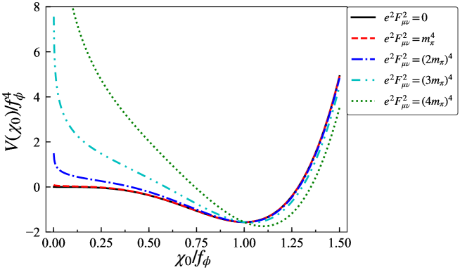
Figure 1: Plot of the dilaton potential in the EM field, as a function of $\chi_{0}/f_{\phi}$, which sketches the screening effect by the created EM-field barrier. The strength of the EM field has been varied in unit of $m_{\pi}^{2}$.

Next, by numerically solving the stationary condition in Eq. (2.24) with the initial condition in Eq. (2.25), the time-dependent dilaton background is evaluated. Fig. 2 shows the EM-field dependence of the time-dependent dilaton background $\chi_{0}(t)$. Note from the chosen initial condition in Eq.(2.25) that in the absence of the EM field, the $\chi_{0}(t)$ keeps constant in time, and stays at the vacuum. By switching on the EM field, the vacuum turns to feel it, and the stationary point is shifted to be a deeper potential minimum specifying a new vacuum, as illustrated in Fig. 1. Thus the dilaton is kicked by the EM field and starts to move to the new vacuum, and then starts to oscillate around the new vacuum. As the EM field increases, the amplitude of the dilaton oscillation becomes larger and larger, and the frequency of the oscillation becomes more rapid as well.

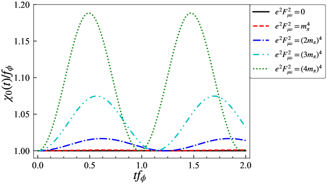
Figure 2: Development of the oscillatory dilaton background $\chi_{0}(t)$ as a function of the normalized time scale $tf_{\phi}$ by increasing the strength of the EM field.

Now, using the time-dependent dilaton background as depicted in Fig. 2, we numerically evaluate the EM dependence of the dynamic oscillatory scale anomalous current in Eq. (3.3). To numerically estimate the anomalous current, we take $E^{x}$ to be $E^{x}=\sqrt{F_{\mu\nu}^{2}}/2$. Fig. 3 shows the EM dependence of the anomalous current. It is now visible that the anomalous current oscillates because of the oscillatory dilaton background. As the EM fields increase, the anomalous current oscillates quicker and the oscillating amplitude becomes larger, in the same manner as the dilaton background does in Fig. 2.

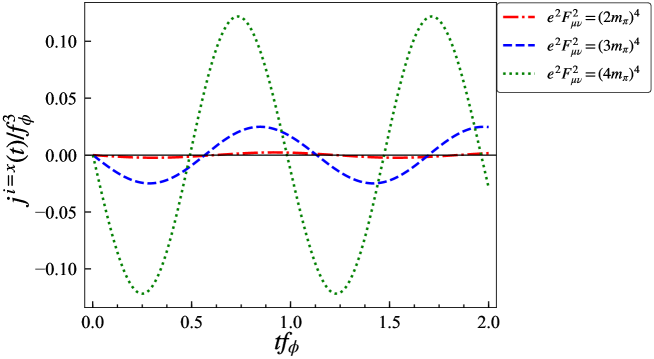
Figure 3: Time evolution of the oscillating scale anomalous current in the EM field, plotted as a function of $tf_{\phi}$.

4.2 Time-dependent dilaton “mass” on the oscillatory background in EM field: nonadiabaticity versus EM screening

So far, we have examined the background level for the oscillatory dilaton physics and anomalous transports. In this subsection, we turn to consider the fluctuation of the dilaton under the oscillating background $\chi_{0}(t)$. From the dilaton potential, the time-dependent effective “mass” for the fluctuating dilaton is evaluated as

$$m_{\chi}^{2}(t) = \frac{\partial^{2}V(\chi)}{\partial\chi^{2}}\Biggl{|}_{\chi=\chi_{0}(t)}$$ (4.2)

$$= \chi_{0}^{2}(t)\frac{m_{\phi}^{2}}{f_{\phi}^{2}}\left[3\log\frac{\chi_{0}(t)}{f_{\phi}}+1\right]+\frac{1}{\chi_{0}^{2}(t)}\frac{\beta(e)}{2e}F_{\mu\nu}^{2}.$$

Note that the fluctuating dilaton rolls along the potential slopes as depicted in Fig. 1, and feels instantaneous curvatures of the potential hills, which correspond to the effective “mass” in Eq.(4.2). Therefore, the time evolution of the effective “mass” highly depends on the initial condition for the oscillating background $\chi_{0}(t)$. We plot the effective “mass” in Fig. 4, varying the initial conditions, such as $\chi_{0}(t=0)/f_{\phi}=1.0,\,0.75,\,0.5$ (the panels (a), (b) and (c), respectively).

Note that even in the absence of the EM field, the dilaton oscillates when we put the dilaton background on a steep hill, far from the stationary point of the dilaton potential. Actually, this is reflected in the effective “mass” in Eq.(4.2), as shown in Fig. 4. When we put the dilaton background much far from the stationary point of the dilaton potential as an initial condition, the effective “mass” more intensely oscillates. Of interest is that the fluctuating dilaton gets a negative mass squared, so that the dilaton (instantaneously) becomes tachyonic, as seen from the panel (c) of Fig. 4. Now, switching on the EM field, the effective “mass” is amplified by the screening effect, as was also observed in the static picture in Fig. 1, and a strong enough EM field finally prevents the dilaton from becoming tachyonic in a whole time-scale, so the dilaton time evolution gets completely stabilized. Actually this drastic screening effect will be significant for the present system, i.e., the hadron phase to keep in the thermal equilibrium, as will be briefly discussed below.

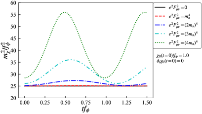
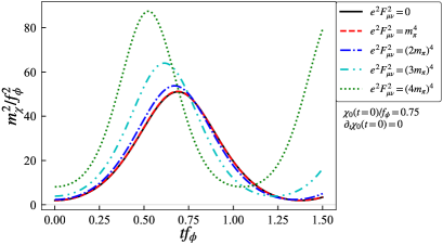
(a) (b)

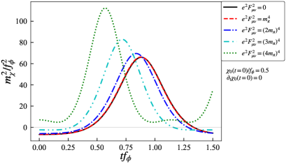
(c)

Figure 4: Time evolution of the effective “mass” of the fluctuating dilaton in Eq.(4.2), for (a) $\chi_{0}(t=0)/f_{\phi}=1.0$, (b) $\chi_{0}(t=0)/f_{\phi}=0.75$ and (b) $\chi_{0}(t=0)/f_{\phi}=0.5$.

First, we should observe that when the dilaton gets tachyonic, the present target system, i.e., the hadron phase is changed from the equilibrium (adiabatic) to be out-of-equilibrium (nonadiabatic), and then nonperturbative particle productions would be generated by the out-of equilibrium processes, to “reheat” the hadron phase by the explosively produced particles (coupled to photons and photons themselves), that is called the tachyonic preheating mechanism Felder:2000hj . In that case, the perturbative estimations for the dilepton production in Eq. (3.10) and the diphoton production in Eq. (3.13) might be too naive, or significantly underestimated (or could be overestimated due to highly nontrivial cancellations). To check this point, we evaluate the non-adiabatic condition,

$$\left|\frac{d}{dt}\left(\frac{1}{m_{\chi}(t)}\right)\right|=\left|\left(\frac{\dot{m}_{\chi}(t)}{m_{\chi}^{2}(t)}\right)\right|\gtrsim 1,$$ (4.3)

which is visualized in the plots depicted in Fig. 5.

The panel (a) shows that at $\chi_{0}(t=0)/f_{\phi}=1.0$ the EM field acts as a catalyzer for the nonadiabaticity of the hadron phase system. This catalysis can be interpreted as the “kick” by the EM field, to make the stationary dilaton highly active. However, for weak EM fields satisfying $e^{2}F_{\mu\nu}^{2}\ll(4.0\,m_{\pi})^{4}$, the system cannot be nonadiabatic. This implies that the “kicks” are still too small to highly accelerate the stable dilaton. Therefore, our perturbative estimates on the anomalous productions in Eqs.(3.10) and (3.13), with such a weak EM field taken into account, are reliable and intact.

For $\chi_{0}(t=0)/f_{\phi}=0.75$, the dilaton is already rolling on the potential and oscillates. As the EM field is turned on and increases, the interference on the nonadiabaticity gets suppressed as depicted in the panel (b) of Fig. 5. Thus, for this initial condition, we find that the EM field serves as an inverse catalysis (i.e. screening) for the nonadiabaticity.

Finally, we examine the case where the initial dilaton is put on a much higher hill in the potential ($\chi_{0}(t=0)/f_{\phi}=0.5$). The panel (c) of Fig. 5 shows that $|\frac{d}{dt}\left(1/m_{\chi}(t)\right)|$ diverges for $e^{2}F_{\mu\nu}^{2}<(3m_{\pi})^{4}$. Note that this is due to the EM effect, but because the dilaton becomes tachyonic as was seen from the panel (c) of Fig. 4. When the EM field reaches a strong strength $F_{\mu\nu}^{2}=(4m_{\pi})^{4}$, the nonadiabaticity gets dismissed, and $|\frac{d}{dt}\left(1/m_{\chi}(t)\right)|$ turns to keep finite values. Thus, eventually even for this initial dilaton, the EM field acts as the screening effect on the nonadiabaticity.

To summarize, as long as the dilaton initially rolls on the potential, which correspond to the cases with the initial conditions (b) and (c), the EM field suppresses the nonadiabaticity to keep driving the hadron phase system into the thermal equilibrium. This is manifested by the screening effect caused by the EM field background, and would be similar to the screening interference phenomenon argued in Refs. Kofman:1997yn ; Czerwinska:2016mbm in a context of backreactions generated by the produced plasma in the preheating scenarios.

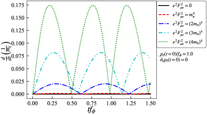
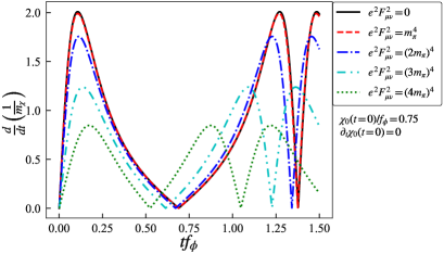
(a) (b)

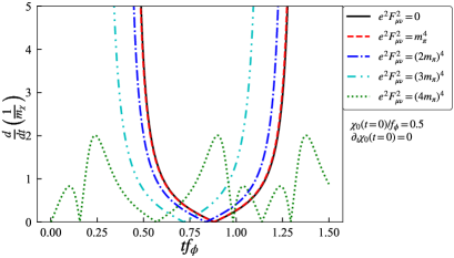
(c)

Figure 5: Plots of the nonadiabatic condition versus the normalized time scale $(tf_{\phi})$, varying the initial conditions: (a) $\chi_{0}(t=0)/f_{\phi}=1.0$, (b) $\chi_{0}(t=0)/f_{\phi}=0.75$ and (c) $\chi_{0}(t=0)/f_{\phi}=0.5$.

5 Summary and discussion

In this paper, we have discussed a scale anomalous current induced from QCD coupled to an EM field, based on a dilaton effective theory reflecting the QCD scale anomaly in a proper way. We first clarified that as long as a QCD dilaton is introduced as if it were a generic singlet scalar universally coupled to the target system, the EM-induced scale anomalous transport takes a universal form, given by the spacetime dependence of a dilaton or a scale factor in a curved spacetime (Eq.(3.3)). The form is completely fixed by the scale/Weyl anomaly structure, whichever one works on a curved or flat spacetime – this was dubbed as an “equivalent theorem”, followed from the frame/Weyl equivalence including the anomaly.

We then claimed that the QCD dilaton, being a dynamical particle contrast to non-dynamical scale factors, would give a discrimination for this robust universality by its dynamics. Our target system has thus been chosen so as to have a nontrivial dynamics of the QCD dilaton: that is a dynamic oscillation in spatially homogeneous hadron phase (with a homogeneous EM field) expected to be created in thermal history of universe, or heavy ion collision experiments. It turned out that the dilaton starts to roll in the potential, and oscillates by a “kick” of the EM field, even if it used to stay at the vacuum. We then observed that the scale anomalous current arises along with the dynamic oscillating dilaton background coupled to the homogeneous EM field, and oscillates as well.

As the phenomenological implication for, e.g., the heavy ion collision experiments, we paid our attention to the anomalous dilepton and diphoton productions generated from the dynamic scale anomalous transport, see Eqs.(3.10) and (3.13). We observed that characteristic peak structures would be seen for those invariant mass distributions, at the effective dilaton mass. This kinematic feature is surely intrinsic, and has never been seen in the ordinary QCD hadron physics. Thus, those particle productions would be crucial signals as indirect detection of the presence of the induced dynamic scale anomalous transport in heavy ion collision experiments.

We also investigated more details of the dynamics of the oscillatory dilaton background. First, we found that in a homogeneous EM field background, the dilaton potential is deformed to have a steeper and deeper well than the one without the EM filed, so that the dilaton field more promptly rolls down to the stationary point of the dilaton potential: the effective dilaton “mass” (i.e., frequency of the oscillation) gets larger and the stationary point (determining the dilaton decay constant) is shifted to be larger (Fig. 1). Then, the time evolution of the oscillating dilaton background and the induced anomalous transport current were analyzed by referring to the potential deformation, where we observed the magnitudes of the oscillations get amplified by increasing the EM strength (Figs. 2 and  3).

The dynamic oscillatory dilaton background also affects the fluctuating dilaton field and can create an out-of-equilibrium state due to the nonadiabatic oscillation, which can be realized when the fluctuating dilaton (instantaneously) gets tachyonic, leading to an explosive nonperturbative particle production (called the tachyonic preheating). We observed that the EM field contributes to the tachyonic preheating as a screening effect, so that the nonadiabaticity gets diluted by a strong EM field (as long as the initial dilaton can have a kinetic energy), see Figs. 4 and 5.

In the present work, we have assumed the presence of a dilatonic meson (identified as the lightest isosinglet scalar meson, $f_{0}(500)$). Note, however, that even if we do not assume such a dialatonic scalar, the form of the lightest isosinglet meson coupling to EM fields is robust, and necessarily couples to the scale anomaly in QCD, as long as the meson is isosinglet. For instance, if we started from an alternative potential form different from the dilatonic potential in Eq. (2.14), we could get a similar diphoton and/or dilepton signal, but different in magnitudes. Precise measurements on the diphoton and/or the dilepton productions might make it possible to probe whether the QCD dilaton picture is viable or not. Thus, the presence of the dynamic scale anomalous transport is a generic consequence of QCD, although the “equivalence theorem” may or may not be applied to the form of the transport current. So, the dynamic scale anomalous transport and/or the dynamic feature of the QCD scalar oscillation might trace one slice of the thermal history of universe, and/or that of the created circumstance in heavy ion collision experiments where strong EM fields are expected to exist.

We have found several dynamic features associated with the presence of the scale anomalous transport induced from QCD in EM field, that would give keys to open a new avenue for the anomalous transport physics in heavy ion collisions, in parallel to the dynamic particle physics that has been developed in the inflation/preheating scenario.

In closing, we give some comments on possible issues left with us.

(1) Incidentally, in a context different from the scale anomaly, it has been argued that the chiral anomaly induced by an EM field also drives similar time-oscillations for condensates (i.e. background fields) of the scalar- and pseudoscalar-quark bilinear (chiral partner) states, to take a spiral form Hayata:2013sea . This time-dependent spiral structure is associated with the dynamic oscillatory chiral currents in the temporal (time) direction induced by the EM field, and hence, called the temporal chiral spiral. The essential difference between the dilaton and the chiral-partner ($\sigma(t)$ and $\pi(t)$) oscillatory backgrounds is that: the former $(\chi(t))$ can be viewed as the chiral singlet component of $\sigma(t)$ and $\pi(t)$; $\chi(t)=\sqrt{\sigma^{2}(t)+\pi^{2}(t)}$, so it keeps constant (which is like an invariant radial length) in time in the temporal chiral spiral because of the chiral invariance. Therefore it cannot be affected by any chiral transformation or anomaly as they act as a phase rotation, that is, the dilaton (radial) mode is driven to oscillate only by the scale transformation (anomaly).

Though being essentially discriminated in QCD with respect to the anomalous transport sources, both two oscillating condensates may share similar phenomenological applications even apart from QCD. As addressed in Ref. Hayata:2013sea , in fact, the temporal chiral spiral can be applied to condensed matter systems such as carbon nanotubes Bockrath:1999 , fractional quantum Hall edge states Wen:1990 and one-dimensional cold-atom systems Guan:2013 . Given this fact, it would be expected that our observation of the oscillating dilaton background as well as the dynamic scale anomalous transport would also be applied to the condensed matter systems. Thus, our findings would also be relevant to give a new insight of the condensed matter physics, which is involved in one of interesting future directions.

(2) The EM beta function can include a nontrivial EM field dependence arising through the up and down quark loops, which would give higher order corrections in powers of $(e^{2}F_{\mu\nu}^{2})$ to the dilaton-photon coupling. In the present study, we have simply neglected such higher order corrections, by assuming a somewhat weak EM field case (compared to the intrinsic QCD scale $\sim$ 1 GeV). However, the higher order corrections might have significantly been sizable in evaluating the dilepton and diphoton productions, and nonadiabaticity for the dilaton oscillation. If it is the case, those production rates would dramatically be enhanced, and the dilaton oscillation would be nonadiabatic even if is “kicked” from the stationary point (corresponding to the initial condition (a), in Fig. 5). In particular, the correction to the latter case could give a great impact on the thermal history of the hadron phase in early universe: the out-of-equilibrium state is induced by the nonadiabatic dilaton oscillation, hence nonperturbative particle productions (perhaps with an excessive entropy production) might happen in the hadron phase. Heavy-ion collision experiments could have a chance to probe such out-of-equilibrium state as well. To rigorously check this point, we need to nonperturbatively compute the dilaton-photon-photon triangle diagram involving the nonperturbative quark propagators. Though this sort of nonperturbative computations has never been done, our current study would motivate people to work on this issue.

(3) Regarding the nonperturbative particle production phenomena, the lattice simulation approach have already started to implement the preheating mechanism inspired by the axion inflation Cuissa:2018oiw . In the axion system, photons can be explosively and nonperturbatively produced by the nonadiabatic axion oscillation via the interaction, $aF\tilde{F}$ with $a$ being the axion field, which has been observed on the lattice. Similarly, it could be plausible on lattice QCD in which a QCD dilaton coupled to diphoton, with the dilaton being assumed only composed of the chiral-singlet part of $u\bar{u}+d\bar{d}$, and measure the nonadiabatic diphoton production, through the interaction $\phi FF$. Such a lattice study will qualitatively and numerically clarify our prediction of the characteristic diphoton production signal as well as nonperturbatively proving the $\phi FF$ coupling, and hence, we would encourage lattice QCD communities to perform this kind of simulations in the future.

(4) Another remark is on the stability of the oscillating dilaton background, i.e. the vacuum in the spatially homogeneous hadron phase. In the present study, we have simply assumed the dilaton vacuum is completely stable, so the dynamic oscillation keeps eternally. However, in reality, the oscillating vacuum should have the lifetime, and decay in a finite time scale (presumably before the Big Bang nucleosynthesis for the thermal history of universe). Or, the oscillation might be ended by a “matter-plasma effect” acting as a backreaction generated during nonperturbative particle productions Dolgov:1989us ; Kofman:1997yn ; Traschen:1990sw ; Kofman:1994rk .

Inclusion of this lifetime can also be done by taking into account possible imaginary parts in the Hamiltonian, which could arise from quantum loop effects, or alternatively along the line of Ref. Huang:2019phi in which the decay of an oscillatory axion-condensed vacuum is studied.

(5) A final remark is about the homogeneity assumption we used in our calculation. Going beyond this assumption would lead to more interesting phenomenological implications. First of all, the possible inhomogeneity in heavy ion collisions would smear the kinematical peak structure predicted in the dilepton and diphoton productions (Eqs.(3.10) and (3.13)), because the dilaton background would become spatially inhomogeneous to make the original resonance form (like a delta function) smeared. This smearing effect might be observed analogously to a collisional broadening in medium, and make the production amplitudes modestly smaller.

Second, if we consider an extreme case of inhomogeneity, namely, a “boundary” in space, the scale anomaly was shown to induce a boundary current (and/or boundary charge density) in the presence of the EM field, as discussed in Chu:2018ksb ; Chu:2018ntx ; Zheng:2019xeu ; Chu:2020mwx ; Chu:2020gwq ; Chernodub:2019blw . It would also be deserved to examine how the “equivalence-theorem” for the scale anomalous transport works even in such an extremely inhomogeneous condition and how the boundary current are understood in the dilaton effective theory.

These issues would be important to give more precise predictions to the anomalous dilepton and diphoton productions, the nonadiabatic oscillatory dilaton “phase” as above, and also other related topics. Their interesting subjects are to be pursued in the future.

References

- (1) D. E. Kharzeev, J. Liao, S. A. Voloshin and G. Wang, Prog. Part. Nucl. Phys. 88, 1 (2016) doi:10.1016/j.ppnp.2016.01.001 [arXiv:1511.04050 [hep-ph]].
- (2) K. Hattori and X. G. Huang, Nucl. Sci. Tech. 28, no. 2, 26 (2017) doi:10.1007/s41365-016-0178-3 [arXiv:1609.00747 [nucl-th]].
- (3) J. Zhao and F. Wang, Prog. Part. Nucl. Phys. 107, 200 (2019) doi:10.1016/j.ppnp.2019.05.001 [arXiv:1906.11413 [nucl-ex]].
- (4) Y. C. Liu and X. G. Huang, Nucl. Sci. Tech. 31, no. 6, 56 (2020) doi:10.1007/s41365-020-00764-z [arXiv:2003.12482 [nucl-th]].
- (5) M. Joyce and M. E. Shaposhnikov, Phys. Rev. Lett. 79, 1193-1196 (1997) doi:10.1103/PhysRevLett.79.1193 [arXiv:astro-ph/9703005 [astro-ph]].
- (6) K. Bamba, Phys. Rev. D 74, 123504 (2006) doi:10.1103/PhysRevD.74.123504 [arXiv:hep-ph/0611152 [hep-ph]].
- (7) K. Kamada and A. J. Long, Phys. Rev. D 94, no.6, 063501 (2016) doi:10.1103/PhysRevD.94.063501 [arXiv:1606.08891 [astro-ph.CO]].
- (8) K. Kamada and A. J. Long, Phys. Rev. D 94, no.12, 123509 (2016) doi:10.1103/PhysRevD.94.123509 [arXiv:1610.03074 [hep-ph]].
- (9) M. M. Anber and E. Sabancilar, Phys. Rev. D 92, no.10, 101501 (2015) doi:10.1103/PhysRevD.92.101501 [arXiv:1507.00744 [hep-th]].
- (10) D. Jiménez, K. Kamada, K. Schmitz and X. J. Xu, JCAP 12, 011 (2017) doi:10.1088/1475-7516/2017/12/011 [arXiv:1707.07943 [hep-ph]].
- (11) V. Domcke, B. von Harling, E. Morgante and K. Mukaida, JCAP 10, 032 (2019) doi:10.1088/1475-7516/2019/10/032 [arXiv:1905.13318 [hep-ph]].
- (12) V. Domcke, Y. Ema and K. Mukaida, JHEP 02, 055 (2020) doi:10.1007/JHEP02(2020)055 [arXiv:1910.01205 [hep-ph]].
- (13) M. S. Turner and L. M. Widrow, Phys. Rev. D 37, 3428 (1988). doi:10.1103/PhysRevD.37.3428
- (14) W. Garretson, G. B. Field and S. M. Carroll, Phys. Rev. D 46, 5346-5351 (1992) doi:10.1103/PhysRevD.46.5346 [arXiv:hep-ph/9209238 [hep-ph]].
- (15) M. M. Anber and L. Sorbo, JCAP 10, 018 (2006) doi:10.1088/1475-7516/2006/10/018 [arXiv:astro-ph/0606534 [astro-ph]].
- (16) A. Hook and G. Marques-Tavares, JHEP 12, 101 (2016) doi:10.1007/JHEP12(2016)101 [arXiv:1607.01786 [hep-ph]].
- (17) K. Choi, H. Kim and T. Sekiguchi, Phys. Rev. D 95, no.7, 075008 (2017) doi:10.1103/PhysRevD.95.075008 [arXiv:1611.08569 [hep-ph]].
- (18) W. Tangarife, K. Tobioka, L. Ubaldi and T. Volansky, [arXiv:1706.00438 [hep-ph]].
- (19) W. Tangarife, K. Tobioka, L. Ubaldi and T. Volansky, JHEP 02, 084 (2018) doi:10.1007/JHEP02(2018)084 [arXiv:1706.03072 [hep-ph]].
- (20) N. Fonseca, E. Morgante and G. Servant, JHEP 10, 020 (2018) doi:10.1007/JHEP10(2018)020 [arXiv:1805.04543 [hep-ph]].
- (21) M. N. Chernodub, Phys. Rev. Lett. 117, no. 14, 141601 (2016) doi:10.1103/PhysRevLett.117.141601 [arXiv:1603.07993 [hep-th]].
- (22) M. N. Chernodub and M. A. Zubkov, Phys. Rev. D 96, no. 5, 056006 (2017) doi:10.1103/PhysRevD.96.056006 [arXiv:1703.06516 [hep-th]].
- (23) M. N. Chernodub, A. Cortijo and M. A. H. Vozmediano, Phys. Rev. Lett. 120, no. 20, 206601 (2018) doi:10.1103/PhysRevLett.120.206601 [arXiv:1712.05386 [cond-mat.str-el]].
- (24) J. J. Zheng, D. Li, Y. Q. Zeng and R. X. Miao, Phys. Lett. B 797, 134844 (2019) doi:10.1016/j.physletb.2019.134844 [arXiv:1904.07017 [hep-th]].
- (25) T. A. DeGrand and K. Kajantie, Phys. Lett. 147B, 273 (1984). doi:10.1016/0370-2693(84)90115-1
- (26) J. E. Kim, S. J. Kim and S. Nam, arXiv:1803.03517 [hep-ph].
- (27) J. E. Kim and S. J. Kim, Phys. Lett. B 783, 357 (2018) doi:10.1016/j.physletb.2018.07.020 [arXiv:1804.05173 [hep-ph]].
- (28) V. Skokov, A. Y. Illarionov and V. Toneev, Int. J. Mod. Phys. A 24, 5925 (2009) doi:10.1142/S0217751X09047570 [arXiv:0907.1396 [nucl-th]].
- (29) W. T. Deng and X. G. Huang, Phys. Rev. C 85, 044907 (2012) doi:10.1103/PhysRevC.85.044907 [arXiv:1201.5108 [nucl-th]].
- (30) J. Bloczynski, X. G. Huang, X. Zhang and J. Liao, Nucl. Phys. A 939, 85 (2015) doi:10.1016/j.nuclphysa.2015.03.012 [arXiv:1311.5451 [nucl-th]].
- (31) Y. Hirono, M. Hongo and T. Hirano, Phys. Rev. C 90, no. 2, 021903 (2014) doi:10.1103/PhysRevC.90.021903 [arXiv:1211.1114 [nucl-th]].
- (32) W. T. Deng and X. G. Huang, Phys. Lett. B 742, 296 (2015) doi:10.1016/j.physletb.2015.01.050 [arXiv:1411.2733 [nucl-th]].
- (33) V. Voronyuk, V. D. Toneev, S. A. Voloshin and W. Cassing, Phys. Rev. C 90, no. 6, 064903 (2014) doi:10.1103/PhysRevC.90.064903 [arXiv:1410.1402 [nucl-th]].
- (34) X. G. Huang, Rept. Prog. Phys. 79, no. 7, 076302 (2016) doi:10.1088/0034-4885/79/7/076302 [arXiv:1509.04073 [nucl-th]].
- (35) T. Vachaspati, Phys. Lett. B 265, 258 (1991). doi:10.1016/0370-2693(91)90051-Q
- (36) K. Enqvist and P. Olesen, Phys. Lett. B 319, 178 (1993) doi:10.1016/0370-2693(93)90799-N [hep-ph/9308270].
- (37) D. Grasso and A. Riotto, Phys. Lett. B 418, 258 (1998) doi:10.1016/S0370-2693(97)01224-0 [hep-ph/9707265].
- (38) D. Grasso and H. R. Rubinstein, Phys. Rept. 348, 163 (2001) doi:10.1016/S0370-1573(00)00110-1 [astro-ph/0009061].
- (39) J. Ellis, M. Fairbairn, M. Lewicki, V. Vaskonen and A. Wickens, JCAP 1909, 019 (2019) doi:10.1088/1475-7516/2019/09/019 [arXiv:1907.04315 [astro-ph.CO]].
- (40) G. N. Felder, J. Garcia-Bellido, P. B. Greene, L. Kofman, A. D. Linde and I. Tkachev, Phys. Rev. Lett. 87, 011601 (2001) doi:10.1103/PhysRevLett.87.011601 [hep-ph/0012142].
- (41) M. A. Shifman, A. I. Vainshtein, M. B. Voloshin and V. I. Zakharov, Sov. J. Nucl. Phys. 30, 711 (1979) [Yad. Fiz. 30, 1368 (1979)].
- (42) R. J. Crewther and L. C. Tunstall, Phys. Rev. D 91, no. 3, 034016 (2015) doi:10.1103/PhysRevD.91.034016 [arXiv:1312.3319 [hep-ph]].
- (43) R. J. Crewther, Universe 6, no.7, 96 (2020) doi:10.3390/universe6070096 [arXiv:2003.11259 [hep-ph]].
- (44) J. Gasser and H. Leutwyler, Annals Phys. 158, 142 (1984). doi:10.1016/0003-4916(84)90242-2
- (45) J. Gasser and H. Leutwyler, Nucl. Phys. B 250, 465 (1985). doi:10.1016/0550-3213(85)90492-4
- (46) J. Schechter, Phys. Rev. D 21, 3393 (1980). doi:10.1103/PhysRevD.21.3393
- (47) A. Salomone, J. Schechter and T. Tudron, Phys. Rev. D 23, 1143 (1981). doi:10.1103/PhysRevD.23.1143
- (48) R. Gomm, P. Jain, R. Johnson and J. Schechter, Phys. Rev. D 33, 801 (1986). doi:10.1103/PhysRevD.33.801
- (49) A. A. Migdal and M. A. Shifman, Phys. Lett. 114B, 445 (1982). doi:10.1016/0370-2693(82)90089-2
- (50) J. M. Cornwall and A. Soni, Phys. Rev. D 32, 764 (1985). doi:10.1103/PhysRevD.32.764
- (51) S. R. Coleman and E. J. Weinberg, Phys. Rev. D 7, 1888 (1973). doi:10.1103/PhysRevD.7.1888
- (52) S. Matsuzaki and K. Yamawaki, Phys. Rev. Lett. 113, no. 8, 082002 (2014) doi:10.1103/PhysRevLett.113.082002 [arXiv:1311.3784 [hep-lat]].
- (53) V. P. Gusynin and V. A. Miransky, Phys. Lett. B 198, 79 (1987) [Ukr. Fiz. Zh. (Russ. Ed. ) 33, 485 (1988)]. doi:10.1016/0370-2693(87)90163-8
- (54) M. Hashimoto and K. Yamawaki, Phys. Rev. D 83, 015008 (2011) doi:10.1103/PhysRevD.83.015008 [arXiv:1009.5482 [hep-ph]].
- (55) S. Matsuzaki and K. Yamawaki, JHEP 1512, 053 (2015) Erratum: [JHEP 1611, 158 (2016)] doi:10.1007/JHEP12(2015)053, 10.1007/JHEP11(2016)158 [arXiv:1508.07688 [hep-ph]].
- (56) Y. L. Li, Y. L. Ma and M. Rho, Phys. Rev. D 95, no. 11, 114011 (2017) doi:10.1103/PhysRevD.95.114011 [arXiv:1609.07014 [hep-ph]].
- (57) A. Kasai, K. i. Okumura and H. Suzuki, arXiv:1609.02264 [hep-lat].
- (58) M. Hansen, K. Langæble and F. Sannino, Phys. Rev. D 95, no. 3, 036005 (2017) doi:10.1103/PhysRevD.95.036005 [arXiv:1610.02904 [hep-ph]].
- (59) T. Appelquist, J. Ingoldby and M. Piai, JHEP 1707, 035 (2017) doi:10.1007/JHEP07(2017)035 [arXiv:1702.04410 [hep-ph]].
- (60) T. Appelquist, J. Ingoldby and M. Piai, JHEP 1803, 039 (2018) doi:10.1007/JHEP03(2018)039 [arXiv:1711.00067 [hep-ph]].
- (61) O. Catà and C. Müller, Nucl. Phys. B 952, 114938 (2020) doi:10.1016/j.nuclphysb.2020.114938 [arXiv:1906.01879 [hep-ph]].
- (62) T. Appelquist, J. Ingoldby and M. Piai, Phys. Rev. D 101, no. 7, 075025 (2020) doi:10.1103/PhysRevD.101.075025 [arXiv:1908.00895 [hep-ph]].
- (63) T. V. Brown, M. Golterman, S. Krøjer, Y. Shamir and K. Splittorff, Phys. Rev. D 100, no. 11, 114515 (2019) doi:10.1103/PhysRevD.100.114515 [arXiv:1909.10796 [hep-lat]].
- (64) J. Khoury and A. Weltman, Phys. Rev. Lett. 93, 171104 (2004) doi:10.1103/PhysRevLett.93.171104 [astro-ph/0309300].
- (65) J. Khoury and A. Weltman, Phys. Rev. D 69, 044026 (2004) doi:10.1103/PhysRevD.69.044026 [astro-ph/0309411].
- (66) K. Fujikawa, Phys. Rev. Lett. 44, 1733 (1980). doi:10.1103/PhysRevLett.44.1733
- (67) K. Fujikawa, Phys. Rev. D 23, 2262 (1981). doi:10.1103/PhysRevD.23.2262
- (68) K. Fujikawa, Phys. Rev. D 48, 3922 (1993). doi:10.1103/PhysRevD.48.3922
- (69) T. Katsuragawa and S. Matsuzaki, Phys. Rev. D 95, no. 4, 044040 (2017) doi:10.1103/PhysRevD.95.044040 [arXiv:1610.01016 [gr-qc]].
- (70) A. Kamada, JHEP 1907, 172 (2019) doi:10.1007/JHEP07(2019)172 [arXiv:1902.05209 [hep-ph]].
- (71) D. E. Kharzeev, L. D. McLerran and H. J. Warringa, Nucl. Phys. A 803, 227 (2008) doi:10.1016/j.nuclphysa.2008.02.298 [arXiv:0711.0950 [hep-ph]].
- (72) K. Fukushima, D. E. Kharzeev and H. J. Warringa, Phys. Rev. D 78, 074033 (2008) doi:10.1103/PhysRevD.78.074033 [arXiv:0808.3382 [hep-ph]].
- (73) G. Basar, D. Kharzeev and V. Skokov, Phys. Rev. Lett. 109, 202303 (2012) doi:10.1103/PhysRevLett.109.202303 [arXiv:1206.1334 [hep-ph]].
- (74) J. S. Schwinger, Phys. Rev. 82, 664 (1951). doi:10.1103/PhysRev.82.664
- (75) M. A. Shifman, A. I. Vainshtein and V. I. Zakharov, Nucl. Phys. B 147, 385 (1979). doi:10.1016/0550-3213(79)90022-1
- (76) M. A. Shifman, A. I. Vainshtein and V. I. Zakharov, Nucl. Phys. B 147, 448 (1979). doi:10.1016/0550-3213(79)90023-3
- (77) L. Kofman, A. D. Linde and A. A. Starobinsky, Phys. Rev. D 56, 3258 (1997) doi:10.1103/PhysRevD.56.3258 [hep-ph/9704452].
- (78) O. Czerwińska, S. Enomoto and Z. Lalak, Phys. Rev. D 96, no. 2, 023510 (2017) doi:10.1103/PhysRevD.96.023510 [arXiv:1701.00015 [hep-ph]].
- (79) T. Hayata, Y. Hidaka and A. Yamamoto, Phys. Rev. D 89, no.8, 085011 (2014) doi:10.1103/PhysRevD.89.085011 [arXiv:1309.0012 [hep-ph]].
- (80) M. Bockrath, D. H. Cobden, J. Lu, A. G. Rinzler, R. E. Smalley, L. Balents, and P. L. McEuen, Nature (London) 397, 598-601 (1999).
- (81) X. G. Wen, Phys. Rev. B 41, 12838 (1990).
- (82) X. -W. Guan, M. T. Batchelor, and A. Lee, Rev. Mod. Phys., 85, 1633 (2013) [arXiv:1301.6446 [cond-mat]].
- (83) J. R. C. Cuissa and D. G. Figueroa, JCAP 06, 002 (2019) doi:10.1088/1475-7516/2019/06/002 [arXiv:1812.03132 [astro-ph.CO]].
- (84) A. D. Dolgov and D. P. Kirilova, Sov. J. Nucl. Phys. 51, 172 (1990) [Yad. Fiz. 51, 273 (1990)].
- (85) J. H. Traschen and R. H. Brandenberger, Phys. Rev. D 42, 2491 (1990). doi:10.1103/PhysRevD.42.2491
- (86) L. Kofman, A. D. Linde and A. A. Starobinsky, Phys. Rev. Lett. 73, 3195 (1994) doi:10.1103/PhysRevLett.73.3195 [hep-th/9405187].
- (87) X. G. Huang, D. E. Kharzeev and H. Taya, Phys. Rev. D 101, no. 1, 016011 (2020) doi:10.1103/PhysRevD.101.016011 [arXiv:1904.08184 [hep-ph]].
- (88) C. S. Chu and R. X. Miao, Phys. Rev. Lett. 121, no.25, 251602 (2018) doi:10.1103/PhysRevLett.121.251602 [arXiv:1803.03068 [hep-th]].
- (89) C. S. Chu and R. X. Miao, JHEP 07, 005 (2018) doi:10.1007/JHEP07(2018)005 [arXiv:1804.01648 [hep-th]].
- (90) C. S. Chu and R. X. Miao, Phys. Rev. D 102, 046011 (2020) doi:10.1103/PhysRevD.102.046011 [arXiv:2004.05780 [hep-th]].
- (91) C. S. Chu and R. X. Miao, [arXiv:2005.12975 [hep-th]].
- (92) M. N. Chernodub and M. A. H. Vozmediano, Phys. Rev. Research. 1, 032002 (2019) doi:10.1103/PhysRevResearch.1.032002 [arXiv:1902.02694 [cond-mat.str-el]].