Go Wide, Then Narrow: Efficient Training of Deep Thin Networks

Abstract

For deploy deep learning models to be deployed into production, they need to be compact enough to meet the latency and memory constraints. A compact model is usually both deep and thin. In this paper, we propose an efficient method to train a very deep and thin network with a theoretic guarantee. Our method is motivated by model compression. It consists of three stages. In the first stage, we sufficiently widen the deep thin network and train it until convergence. In the second stage, we use this well-trained deep wide network to warm up (or initialize) the original deep thin network. This is achieved by letting the thin network imitate the immediate outputs of the wide network from layer to layer. In the last stage, we further fine tune this already well warmed-up deep thin network. The theoretical guarantee is established by using mean field analysis. It shows that the proposed method is provably more efficient than training deep thin networks from scratch by backpropagation. We also conduct large-scale empirical experiments to validate our approach. By training with our method, ResNet50 can outperform ResNet101, and $\text{BERT}_{\text{BASE}}$ can be comparable with $\text{BERT}_{\text{LARGE}},$ where both the latter models are trained via the standard training procedures as in the literature.

1 Introduction

In many machine learning applications, in particular, language modeling and image classification, it is becoming common to dramatically increase the model size to achieve significant performance improvement (he2016deep; devlin2018bert; brock2018large; raffel2019exploring; efficientnet2019). To enlarge a model, we can simply make it much deeper or wider. In the current days, a big deep learning model may involve millions or even billions of parameters. These big models are often trained over large computation clusters with hundreds or thousands of computational nodes.

However, despite their impressive performance, it is almost impossible to directly deploy these big models to resource-limited devices such as mobile phones. To remedy this issue, there has been an increasing interest in developing model compression techniques. Typical solutions include pruning, quantization and knowledge distillation (ba2014deep; han2015learning; hinton2015distilling; courbariaux2015binaryconnect; rastegari2016xnor). In practice, these techniques usually can produce sufficiently compact models without significant drop of accuracy.

Then, a question naturally arises: When our ultimate goal is to have a compact model, why not directly train this model from the beginning? Direct training seems to be more efficient than training a big model first and then compressing it to the target size. We are particularly interested in investigating deep thin networks, a special kind of compact models. That is because most compact models are both deep and thin. A compact model even has to be sufficiently deep since a deep model is supposed to extract hierarchical high-level representations from inputs while a shallow model not (le2012building; allen2020backward). On the other hand, a model to be deployed does not have to be that wide. It is generally observed that a wider model is easier to train. That is because its loss surface is smoother and nearly convex (li2018visualizing; du2018gradient). After training, however, the wide network can be largely pruned while reserving accuracy.

In this paper, we propose a generic algorithm to train a deep thin network with theoretic guarantee. Our method is motivated by model compression. It consists of three stages (Figure 1 and Algorithm 1). In the first stage, we widen the deep thin network to obtain a deep wide network and train it until convergence. In the second stage, we use this well trained deep wide network to warm up or initialize the original deep thin network. In the last stage, we train this well initialized deep thin network as usual until convergence. Empirical studies show that the proposed approach significantly outperforms the baseline of training a deep thin network from scratch. By training with our approach, ResNet50 (he2016deep) can outperform normally trained ResNet101 as in the literature, and $\text{BERT}_{\text{BASE}}$ (devlin2018bert) can be comparable with $\text{BERT}_{\text{LARGE}}.$

The key component of our method is its second stage. In this stage, the thin network is gradually warmed up by imitating the intermediate outputs of the well trained wide network from bottom to top. This is like curriculum learning, where a teacher breaks down an advanced learning topic to many small tasks, and then student learn these small tasks one by one under the teacher’s stepwise guidance. The big issue here is that the wide and thin networks differs in the output dimension. To overcome this issue, we insert a pair of linear transformations between any two adjacent layers in the thin network. One is used to increase the dimension of its layer output to match the dimension of the wide network, and the other to reduce back the dimension. Then, the dimension expanded output from the thin network can be compared with the output from the wide network. After this stage, we merge all adjacent linear layers in the thin network such that its architecture stays unchanged while it has been well initialized. Training a deep thin network is a highly nonconvex optimization. A a good initialization is all we need to achieve a good training result.

We establish theoretical guarantee for our method using the mean field analysis of neural networks (song2018mean; araujo2019mean). Based on our theoretic results, when training a deep thin network from scratch, the bound of training error increases exponentially as the network goes deeper (Proposition 3.3). In contrast, for our method, we are able to establish an error bound that increases only linearly with the network depth (Theorem 3.5). The analysis relies on the special layerwise initialization scheme in our method to avoid the exponential dependency on the network depth, which does not hold for other model compression techniques, in particular, knowledge distillation and its variants (ba2014deep; hinton2015distilling).

We organize this paper as follows. Our algorithm is illustrated in Section 2. The main theoretic results built upon mean field analysis for neural networks are introduced in Section 3. All the proof details are provided in Appendix. Related work are discussed in Section 4. Large-scale experiments on image classification and language modeling are presented in Section 5. We conclude this paper with discussions in Section 6.

2 Algorithm

Let us denote by $S=\{S_{1},S_{2},\dots,S_{n}\}$ a deep thin network that we want to train, where $S_{i}$ denotes the building block at the $i$-th layer of $S.$ For an input $x,$ the output of network $S$ is given as $S(x)=(S_{n}\circ S_{n-1}\circ\cdots\circ S_{1})(x)=S_{n}(S_{n-1}(\cdots S_{2}(S_{1}(x))\cdots)).$ In a feed forward network, a building block can be a hidden layer or a group of hidden layers. However, in many other models, the structure of a building block can be much more complicated. In a model for image classification, a building block usually contains convolution, pooling, and batch normalization (he2016deep); in models for language processing, a building block may include multi-head attention, feed-forward network, and layer normalization (vaswani2017attention).

Stage 1: Wide learning. In this stage, we first construct a deep wide network $B=\{B_{1},\dots,B_{n}\},$ where building block $B_{i}$ is obtained by widening building block $S_{i}$ in the deep thin network $S.$ We then train this deep wide network $B$ until convergence. In general, a wider network is easier to train. How to make a specific network wider and how much wider are case by case. For a feed forward network, we can make it wider by increasing the widths of its hidden layers. For a convolution network, we can make it wider by introducing more filters. For a transformer like model, it can be widened from multiple dimensions, including using a larger number of hidden states, more self-attention heads, or more hidden neurons in its feed forward module.

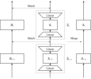
Figure 1: Illustration of WIN. Left panel: wide network $B$ with building blocks $B_{i}$ obtained by widening $S_{i}$ in the thin network $S$. Middle panel: network $\bar{S}$ obtained by inserting appropriately sized linear transformation pairs between any two adjacent building blocks $S_{i-1}$ and $S_{i}$ in $S$. Right panel: merge all adjacent linear transformations in $\bar{S}$ to reduce the network architecture to $S$.

Stage 2: Narrow learning. In this stage, we first construct a new network $\bar{S}$ by inserting a pair of appropriately sized linear transformations $M_{i}=\{M_{i,1},M_{i,2}\}$ between any two adjacent building blocks $S_{i}$ and $S_{i+1}$ in the thin network $S$ (see Figure 1 for an illustration of $\bar{S}$). The first linear transformation $M_{i,1}$ increases the output dimension of $S_{i}$ to match the dimension of $B_{i}$ in the wide network $B,$ and the second linear transformation $M_{i,2}$ reduces the dimension back. That is, after two sequential linear mappings, the output dimension stays the same.

Now, let us look at the new network $\bar{S}$ in a slightly different view. Formally, the network $\bar{S}$ can be written as $\bar{S}=\{S_{1},M_{1},S_{2},M_{2},S_{3},\dots,M_{n-1},S_{n}\}.$ We may group the modules in $\bar{S}$ as follows: $\bar{S}_{1}=\{S_{1},M_{1,1}\},$ $\bar{S}_{i}=\{M_{i-1,2},S_{i},M_{i,1}\}$ for all $i$ in $\{2,\dots,n-1\},$ and $\bar{S}_{n}=\{M_{n-1,2},S_{n}\}.$ Thus, we have $\bar{S}=\{\bar{S}_{1},\bar{S}_{2},\dots,\bar{S}_{n}\}.$

Next, for $i=1,\dots,n-1,$ we sequentially train a set of subnetworks $\bar{S}^{(i)}=\{\bar{S}_{1},\dots,\bar{S}_{i}\}$ by minimizing the output discrepancy between $\bar{S}^{(i)}$ and subnetwork $B^{(i)}=\{B_{1},\dots,B_{i}\}$ in the wide network $B.$ The instances in the training data are used as the inputs here. Note that $B^{(i)}$ is not trained here since the entire network $B$ has been trained in the first stage. In addition, during this sequential training, the trained $\bar{S}^{(i)}$ is served as initialization when proceeding to training $\bar{S}^{(i+1)}.$ There are many ways to measure the output discrepancy of two networks. Typical choices include the mean squared error and Kullback-Leibler divergence.

To achieve better performance, when training each subnetwork $\bar{S}^{(i)}$, we may restart multiple times. In each restart, the most recently added building block $S_{i}$ is reinitialized randomly. Finally, we choose the trained network which best mimics $B^{(i)}$ to proceed to training $\bar{S}^{(i+1)}.$

Algorithm 1 go WIde, then Narrow (WIN)

  Input: thin network $S=\{S_{1},\dots,S_{n}\}$; training data

  

   Stage 1: Wide learning. Construct a wide network $B=\{B_{1},\cdots,B_{n}\},$ where each $B_{i}$ is obtained by widening $S_{i}$ in network $S$, and train $B$ until convergence.

  

  Stage 2: Narrow learning. Construct another network $\bar{S}=\{\bar{S}_{1},\dots,\bar{S}_{n}\},$ where each $\bar{S}_{i}$ can be regarded as wrapping up $S_{i}$ by two appropriately sized linear transformations to match the output dimension of $B_{i}.$

  

  for $i=1$ to $n-1$ do

     Train subnetwork $\bar{S}^{(i)}=\{\bar{S}_{1},\dots,\bar{S}_{i}\}$ by minimizing the output discrepancy between $\bar{S}^{(i)}$ and subnetwork $B^{(i)}=\{B_{1},\dots,B_{i}\}$ from the wide network $B$.

  end for

  

  Stage 3: Fine-tuning and merging. Use the training labels to fine tune network $\bar{S}^{(n)}=\bar{S}$, and then merge all adjacent linear layers in $\bar{S}.$

Stage 3: Fine-tuning and merging. This is the final stage of our method. Up till now, the network $\bar{S}^{(n)}=\bar{S}$ has been well initialized. Next we further fine tune this network using the training labels. Then, we merge all adjacent linear transformations in $\bar{S}$, including the native linear layers residing in its building blocks, such that $\bar{S}$ is reduced back to the architecture of the original deep thin network $S$ (see the illustration in Figure 1). Until then our algorithm is done. Optionally, one may restart fine-tuning several times, and then choose the model which has the least training error. This greedy choice usually works since a thin model is supposed to have a strong regularization effect on its own.

3 Theoretical Analysis

In this section, we present theoretical analysis on why this layerwise imitation fashion in our algorithm improves training. The basic intuition is that the layerwise imitation breaks the learning of the deep thin network into a sequence of shallow subnetworks training, and hence avoids backpropagation through the entire deep thin network from top to bottom, making it more suitable for very deep networks.

We start with a brief informal overview of our key results before presenting the rigorous technical treatment in Section 3.1. Our results can be summarized as follows.

1. If we train the deep thin network $S$ directly using backpropagation, the output discrepancy between the trained thin network $S$ and the wide network $B$ is

   $$O(n\exp(n)/\sqrt{m}),$$

   where $n$ and $m$ denote the depth and width of the deep narrow network, respectively. The exponential term $\exp(n)$ is due to the gradient vanishing/exploding problem and reflects the fundamental difficulty of training very deep networks.

2. In contrast, if we train the deep thin network $S$ through the layerwise imitation of its deep wide version $B$ as shown in Algorithm 1, the output discrepancy between $S$ and $B$ then becomes

   $$O\left(n/\sqrt{m}\right),$$

   which depends on the depth $n$ only linearly. This is in sharp contrast with the exponential dependency of the standard backpropagation.

Therefore, by going wide and then narrow (WIN) and following our layerwise imitation strategy, we provide a provably better approach for training deep thin networks than the standard backpropagation. It resolves the well-known gradient vanishing/exploding problem in very deep and thin networks, and avoids the exponential dependency on the depth in deep backpropagation.

3.1 Assumptions and Theoretical Results

Our analysis is built on the theory of mean field analysis of neural network (e.g., song2018mean; araujo2019mean; nguyen2020rigorous). We start with the formulation of deep mean field network formulated by araujo2019mean.

For notation, assume $S^{m}=\left\{S_{1}^{m},S_{2}^{m},\cdots,S_{n}^{m}\right\}$ and $B^{M}=\left\{B_{1}^{M},B_{2}^{M},\cdots,B_{n}^{M}\right\}$ are the thin and wide networks of interest, where we add the superscribe $m$ and $M$ to denote the number of neurons in each layer of the thin and wide networks, respectively. We assume the $i$-th layer of $S^{m}$ and $B^{M}$ are

$$S_{i}^{m}(\text{{z}})=\frac{1}{m}\!\sum_{j=1}^{m}\!\sigma\!\!\left(\text{{z}},\boldsymbol{\theta}_{i,j}^{S}\right), B_{i}^{M}(\text{{z}})=\frac{1}{M}\!\sum_{j=1}^{M}\!\sigma\!\!\left(\text{{z}},\boldsymbol{\theta}_{i,j}^{B}\right),$$

where $\boldsymbol{\theta}_{i,j}^{S}$ and $\boldsymbol{\theta}_{ij}^{B}$ are the weights of the thin and wide models, respectively. Here we also define

$$\sigma(\text{{z}},\boldsymbol{\theta})=\boldsymbol{\theta}_{1}^{\top}\sigma_{+}(\text{{z}}^{\top}\boldsymbol{\theta}_{0}),\ \ \ \boldsymbol{\theta}=[\boldsymbol{\theta}_{0},\boldsymbol{\theta}_{1}],$$

where $\sigma_{+}(\cdot)$ is some commonly used nonlinear element-wise mapping such as sigmoid.

In order to match the dimensions of the thin and wide models, we assume the input and output of both $S_{i}^{m}(\text{{z}})$ and $B_{i}^{M}(\text{{z}})$ of all the layers (except the output) all have the same dimension $d$, so that $\text{{z}}\in\mathbb{R}^{d}$ and $\boldsymbol{\theta}_{i,j}^{S},\boldsymbol{\theta}_{i,j}^{B}\in\mathbb{R}^{(d+1)\times d}$ for all the neurons and layers. In practice, this can be ensured by inserting linear transform pairs as we have described in our practical algorithm (so that the $S_{i}^{m}$ corresponds to the $\bar{S}_{i}$ in Figure1). In addition, for the sake of simplicity, the dimension of the final output is assumed to be one.

Giving a dataset $\mathcal{D}=\{\textbf{x}_{i},y\}_{i}$, we consider the regression problem of minimizing the mean squared error:

$$\mathcal{L}(F)=\mathbb{E}_{(\textbf{x},y)\sim\mathcal{D}}\left[\left(F(\textbf{x})-y\right)^{2}\right],$$ (1)

via gradient descent with step size $\eta$ and a proper random initialization.

Assumption 3.1.

Denote by $B_{\mathrm{GD}}^{m}$ and $S_{\mathrm{GD}}^{M}$ the result of running stochastic gradient descent on dataset $\mathcal{D}$ with a constant step size $\eta>0$, for a fixed $T$ steps.

For both models, we initialize the parameters $\{\boldsymbol{\theta}_{i,j}^{S}\}_{j\in[m]}$ and $\{\boldsymbol{\theta}_{i,j}^{B}\}_{j\in[M]}$ in the $i$-th layer by drawing i.i.d. samples from a distribution $\rho_{i}$. We suppose $\rho_{i}$ is absolute continuous and has bounded domain for $i\in[n]$.

We need some mild regularization conditions, which are common in neural network analysis (song2018mean; araujo2019mean).

Assumption 3.2.

Suppose the data and label in $\mathcal{D}$ are bounded, i.e. $\left\|\textbf{x}\right\|\leq c$ and $\left|y\right|\leq c$ for some $c<\infty$. And suppose the activation function $\sigma_{+}$ and its first and second derivatives are bounded.

The following result controls the discrepancy between thin and wide models $S^{m}_{\mathrm{GD}}$ and $B_{\mathrm{GD}}^{M}$, which yields a rather loose bound that grows exponentially with the depth $n$ of the network. This is because the gradient descent backpropagates through the $n$-layer deep networks, causing the gradient vanishing/exploding problem.

Define the output discrepancy between two models $S$ and $B$ by

$${\mathbb{D}}[S,B]=\sqrt{\mathbb{E}_{\textbf{x}\sim\mathcal{D}}\left[\left(S(\textbf{x})-B(\textbf{x})\right)^{2}}\right].$$

Proposition 3.3.

(Output Discrepancy Between the Thin Network and the Wide Network Trained by Stochastic Gradient Descent) Under assumption 3.2 and 3.1, we have

$${\mathbb{D}}[S^{m}_{\mathrm{GD}},B^{M}_{\mathrm{GD}}]=\mathcal{O}_{p}\left(n\exp(\exp(n))\left(\frac{1}{\sqrt{m}}+\frac{1}{\sqrt{M}}+\sqrt{\eta}\right)\right),$$

where $\mathcal{O}_{p}(\cdot)$ denotes the big O notation in probability, and the randomness is w.r.t. the random initialization of gradient descent, and the random mini-batches of stochastic gradient descent.

Because the $m$ is small and $n$ is large for deep thin networks, the term $n\exp(\exp(n))m^{-1/2}$ can be the dominating term in the bound above. This result reveals a curse of depth when we train deep thin networks directly using gradient descent. In contrast, as we show in sequel, our layerwise imitation yields a loss that avoids the exponential dependency.

Breaking the Curse of Depth with Layerwise Imitation

Now we analyze how our layerwise imitation algorithm helps the learning of deep thin networks.

Assumption 3.4.

Denote by $S^{m}_{\mathrm{WIN}}$ the result of mimicking $B_{\mathrm{GD}}^{M}$ following Algorithm 1. When training $S_{\mathrm{WIN}}^{m}$, we assume the parameters of $S^{m}_{\mathrm{WIN}}$ in each layer are initialized by randomly sampling $m$ neurons from the the corresponding layer of the wide network $B_{\mathrm{GD}}^{M}$. Define $B^{M}_{\mathrm{GD},[i:n]}=B_{n}^{M}\circ\cdots B_{i}^{M}$.

Theorem 3.5.

(Main Result) Assume all the layers of $B^{M}_{\mathrm{GD}}$ are Lipschitz maps and all its parameters are bounded by some constant. Under the assumptions 3.1, 3.2, 3.4, we have

$${\mathbb{D}}[S_{\mathrm{WIN}}^{m},B^{M}_{\mathrm{GD}}]=\mathcal{O}_{p}\left(\frac{\ell_{B}n}{\sqrt{m}}\right),$$

where $\ell_{B}=\max_{i\in[n]}\left\lVert B^{M}_{\mathrm{GD},[i+1:n]}\right\rVert_{\mathrm{Lip}}$ and $\mathcal{O}_{p}(\cdot)$ denotes the big O notation in probability, and the randomness is w.r.t. the random initialization of gradient descent, and the random mini-batches of stochastic gradient descent.

Note that because is expected that the wide network $B^{M}_{\mathrm{GD}}$ is easy to train. It is expected to be close to the unknown true map between the data input and output and behave nicely, its maximum Lipschitz constant $\ell_{B}$ is small and hence does not explode with $n$. Therefore, the bound of $S_{\mathrm{WIN}}^{m}$ depends on the depth $n$ (approximately) linearly. and at most exponentially. An important future work is to develop rigours bounds for $\ell_{B}$.

4 Related Work

Our method is deeply inspired by MobileBERT (zhiqing2020mobile), which is a highly compact model BERT variant designed for mobile applications. In its architecture, the original BERT building block is replaced with a bottleneck structure. To train it, MobileBERT is first initialized by imitating the outputs of a well trained large BERT from layer to layer and then fine tuned. The main difference between MobileBERT and the proposed method here is that in MobileBERT linear transformations are introduced with the bottleneck structures so they are part of the model and cannot be cancelled out by merging as in our method.

FitNets (romero2014fitnets) also aim at training deep thin networks. In this work, a student network is first partially initialized by matching the output from its some chosen layer (guided layer) to the output from some chosen layer (hint layer) of a teacher network. The chosen guided and hint layers do not have to be at the same depth since the teacher network is chosen to be shallower than the student network. Then, the whole student network is trained via knowledge distillation. The matching is implemented by minimizing a parameterized mean squared loss in which a regressor is applied to the student’s output such that its output can match the size of the teacher’s output. The main difference between FitNets and our method is that the introduced regressor in FitNets is not part of the student network.

This kind of teacher-student methods can be traced back to knowledge distillation and its variants (ba2014deep; hinton2015distilling). The basic idea in knowledge distillation is to use both true labels and the outputs from a cumbersome model to train a small model. In the literature, the cumbersome model is usually referred to as teacher, and the small model student. The loss based on the teacher’s outputs, that is, the so-called distillation loss, is linearly combined with the true labels based training loss as the final objective to train the student model. In the variants of knowledge distillation, the intermediate outputs from the teacher model are further used to construct the distillation loss which is parameterized as in FitNets. Unlike knowledge distillation, our method uses a teacher model to initialize a student model rather than constructing a new training objective. After the initialization, the student model is trained as usual. Based on such a special initialization manner, we are able to establish theoretic guarantee for our approach.

Our theory is built upon the mean field analysis for neural networks, which is firstly proposed by song2018mean to study two-layer neural networks and then generalized to deep networks by araujo2019mean. The general idea of mean field analysis is to think of the network as an interacting particle system, and then study how the behavior of the network converges to its limiting case (as the number of neurons increases). It is shown by araujo2019mean that as the depth of a network increases, the stochasticity of the system increases at an exponential scale with respect to its depth. This characterizes the problem of gradient explosion or vanish. On the other hand, they also establish the results which suggest that increasing the width of the network helps the propagation of gradient, as it reduces the stochasticity of the system. In our method, we first train a wide network that helps the propagation of gradients, and then let the thin network mimic this wide network from layer to layer. Consequently, the negative influence of depth decreases from exponential to linear.

5 Experiments

We conduct empirical evaluations by training state of the arts neural network models for image classification and natural language modeling. Our baselines include vanilla training methods for these models as shown in the literature as well as knowledge distillation. In addition, in what follows, following the convention in the literature and for the sake of convenience, we refer to the wide model in our method as teacher, and the thin model as student.

5.1 Image Classification

We train the widely used ResNet models (he2016deep) on the ImageNet dataset (imagenet15) using our apporach and baseline methods.

5.1.1 Setup

Models.

ResNet is build on a list of bottleneck layers (he2016deep). Each bottleneck layer consists of three modules: a projection 1x1 convolution to reduce the channel size to 1/4 of the input channels, a regular 3x3 convolution, and a final expansion 1x1 convolution to recover the channel size. The wide teacher model used in our method is constructed by increasing the channel size of the 3x3 convolution as in (zagoruyko2016wide), and the remaining two 1x1 convolutions simply keep the increased channel size without projection or expansion.

The models that we evaluate include ResNet50, ResNet101 and their reduced versions: ResNet50-1/2, ResNet50-1/4, ResNet101-1/2 and ResNet101-1/4. For each model’s reduced version, we apply the same reducing factor to all layers in that model. For example, ResNet50-1/2 means that the channel size of every layer in this model is half the channel size of the corresponding layer in ResNet50. The complexity numbers including FLOPs and parameter sizes for different models are collected in Table 1 for reference.

Vanilla training setting.

We follow the training settings in (he2016deep). Each ResNet variant is trained with 90 epochs using SGD with momentum 0.9, batch norm decay 0.9, weight decay 1e-4, and batch size 256. The learning rate is linearly increased from 0 to 0.1 in the first 5 epochs, and then reduced by 10x at epoch 30, 60 and 80.

WIN setting.

We naturally split ResNet into four big chunks or building blocks with respect to the resolution change, that is, with separations at conv2_x, con3_x, conv4_x, and con5_x. In the first stage of our method, the teacher network is constructed as 4x larger (in terms of the channel size of the 3x3 convolutions) than the corresponding student network, and trained with the vanilla setting. In the second stage, for training each building block in the student network, we run 10 epochs by minimizing the mean squared error between the output of the teacher and student network. The optimizer is SGD with momentum 0.9. The learning rate decayed from 0.1 to 0 under the cosine decay rule. After that, we fine tune the student network for 50 epochs by minimizing the Kullback-Leibler divergence from the teacher logits to student logits, with the learning rate decayed from 0.01 to 0 under the cosine decay rule. Note that the total number of training epochs here is 90, which is the same as in the vanilla training. We do not apply weight decay in the last two stages since the compact architecture of a thin network has already implied a strong regularization.

Table 1: Model complexity comparison between the teacher and student models.

	Teacher		Student
	FLOPs	Params	FLOPs	Params
ResNet50	11B	68M	4.1B	26M
ResNet50-1/2	2.9B	18M	1.1B	6.9M
ResNet50-1/4	0.75B	4.7M	0.29B	2.0M
ResNet101	23B	127M	7.9B	45M
ResNet101-1/2	5.8B	32M	2.0B	12M
ResNet101-1/4	1.5B	8.3M	0.53B	3.2M

5.1.2 Results

The evaluation results are collected in Table 2. The numbers listed in the table cells are the top-1 accuracy on the ImageNet dataset from the models trained by different methods: our method, the vanilla training, and knowledge distillation. The results show that our method significantly outperforms the baseline methods. Moreover, we would like to point out that ResNet50 trained by our method achieves an accuracy of $78.4\%$ which is even higher than the accuracy of $77.5\%$ from ResNet101 trained by the vanilla approach.

We conduct an ablation study to demonstrate the effect of the teacher model size. The results are shown in Table 3. For ResNet50, the 2x teacher performs almost equally well as the 4x teacher. The same observation holds for their students. However, for the thinner models ResNet50-1/2 and ResNet50-1/4, the models trained by the 2x teacher are worse than the models trained by the 4x teacher. We do not try an even larger teacher such as the 6x one because of the computational cost.

Table 2: ImageNet top-1 accuracy $(\%)$ by the models trained by the vanilla setting, knowledge distillation (KD), and our method.

Model	Vanilla	KD	WIN
ResNet50	76.2	76.8	78.4
ResNet50-1/2	72.2	72.9	74.6
ResNet50-1/4	64.2	65.1	66.4
ResNet101	77.5	78.0	79.1
ResNet101-1/2	74.6	75.5	76.8
ResNet101-1/4	68.1	69.1	69.7

Table 3: ImageNet top-1 accuracy $(\%)$ by different size teachers and their students trained with our method.

	2x		4x
	Teacher	Student	Teacher	Student
ResNet50	78.4	78.4	78.6	78.2
ResNet50-1/2	76.0	74.6	77.6	75.0
ResNet50-1/4	70.5	66.4	74.4	67.5

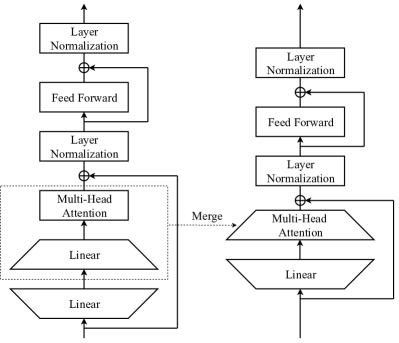
Figure 2: Adding linear transformation pairs into a thin BERT model. Left panel: a pair of linear transformation are inserted between any two adjacent transformer blocks. Right Panel: the linear transformation right next to the multi-head attention module (see the dashed box in the left panel) is merged before the training in the second stage, i.e., the stage of narrow learning, while the remaining linear transformation will be merged after fine-tuning when the whole training procedure is done. Thus, finally, the trained model has the exact same network architecture and number of parameters as the original thin model.

5.2 Language Modeling

In this task, we train BERT (devlin2018bert), the state-of-the-art pre-training language model, using our method as well as the baseline methods as in the image classification tasks. Following devlin2018bert, we firstly pre-train the BERT model using BooksCorpus (zhu2015aligning) and the Wikipedia corpus. Then we fine-tune this pre-trained model and evaluate on the Stanford Question Answering Dataset (SQuAD) 1.1 and 2.0 (rajpurkar2016squad).

5.2.1 Setup

Table 4: The results on the SQuAD dev datasets from the BERT models trained by our method, vanilla training and knowledge distillation (KD). †marks our runs with the official code.

	SQuAD 1.1		SQuAD 2.0
Model	Exact Match	F1	Exact Match	F1
BERT${}_{\text{BASE}}$ (devlin2018bert)	80.8	88.5	74.2†	77.1†
BERT${}_{\text{LARGE}}$ (devlin2018bert)	84.1	90.9	78.7	81.9
Teacher	85.5	91.9	80.3	83.2
BERT${}_{\text{BASE}}$ (Vanilla)	83.6	90.5	77.9	80.4
BERT${}_{\text{BASE}}$ (KD)	84.2	90.8	78.9	81.4
BERT${}_{\text{BASE}}$ (WIN)	85.5	91.8	79.6	82.5

Models.

The model that we are going to train here is BERT${}_{\text{BASE}}$. It takes token embeddings as its inputs and contains 12 transformer blocks (vaswani2017attention). Each transformer block consists of one multi-head self-attention module and one feed forward network module, which are followed by layer normalization and connected by skip connections respectively. On top of the transformer blocks, there is a classifier layer to make task-specific predictions.

The teacher model for our method is constructed by simply doubling the hidden size of every transformer block and also the width of every feed forward module in BERT${}_{\text{BASE}}$. We keep the size of the teacher model’s embedding the same as BERT${}_{\text{BASE}}$’s and add a linear transformation right after teacher model’s embedding to match its hidden size. Thus, the student model described below and the wider teacher model can share the same token embeddings as their inputs.

The way to construct the student model is illustrated in Figure 2. Specifically, taking the canonical BERT${}_{\text{BASE}}$ model, we insert a pair of linear transformations between any two adjacent transformer blocks. We also put one extra linear layer over the last transformer block of BERT${}_{\text{BASE}}$. The output size of the lower linear transformation is designed to be the same as the output size of teacher model’s transformer block, i.e., the teacher model’s hidden size. To more efficiently train this student model, before the training, we merge the upper linear transformation into the fully-connected layers inside the multi-head attention module. After training, we can further merge the remaining lower linear transformation into the multi-head attention module. Similarly, we can also merge the extra linear transformation over the last transformer block into the final classifier layer. Hence, the final student model has the exact same network architecture and number of parameters as BERT${}_{\text{BASE}}$.

Vanilla training setting.

There are two training phrases for the BERT models: pre-training and fine-tuning. In the pre-training phrase, we train the model on the masked language modeling (MLM) and next sentence prediction (NSP) tasks using BookCorpus and Wikipedia corpus for 1 million steps with batch size of 512 and sequence length of 512. We use the Adam optimizer with the learning rate of 1e-4, $\beta_{1}$ = 0.9, $\beta_{2}$ = 0.999, weight decay of 0.01. The learning rate is linearly warmed up in the first 10,000 steps, and then linearly decayed. After pre-training, we enter the fine-tuning phrase. In this phrase, we fine tune all the parameters using the labeled data for a specific downstream task.

WIN setting.

In the first stage of our method, we train the 2x wider teacher model using the vanilla method. In the second stage, we first copy the teacher model’s token embeddings to the student model, and then progressively warm up the student’s transformer blocks from layer to layer. In each step of this stage, we minimize the mean squared error between the output of the linear transformation after the student’s transformer block, and the output of the teacher’s corresponding transformer block. We train the first transformer block for 10k steps, the second for 20k steps until the 12th for 120K steps. Note that BERT${}_{\text{BASE}}$ has 12 transformer block layers in total. Now we enter the fine-tuning stage. We follow the same vanilla training setting to pre-train this warmed-up model on MLM and NSP tasks. Finally, we fine tune the model for downstream tasks (no knowledge distillation is employed here).

5.2.2 Results

We evaluate the models using the SQuAD 1.1 and 2.0 datasets. Results are shown in Table 4. Note that BERT${}_{\text{BASE}}$ trained using our vanilla setting here outperforms BERT${}_{\text{BASE}}$ (devlin2018bert) by a large margin. The reason for the improvement is that we pre-train the model with sequence length of 512 for all steps, while devlin2018bert pre-train the model with sequence length of 128 for 90% of the steps and sequence of 512 for the rest 10% steps. The better training result establishes a stronger baseline. BERT${}_{\text{BASE}}$ trained by our method further beats this stronger baseline by 1.9 exact match score and 1.3 F1 score on SQuAD 1.1, and 1.7 exact match score and 2.1 F1 score on SQuAD 2.0. Actually, BERT${}_{\text{BASE}}$ trained by our method is comparable with BERT${}_{\text{LARGE}}$ by vanilla training.

Table 5: The results on the SQuAD 1.1 dev dataset from the BERT${}_{\text{BASE}}$-1/2 models trained by our method and baselines.

Model	Exact Match	F1
BERT${}_{\text{BASE}}$-1/2 (Vanilla)	78.9	86.3
BERT${}_{\text{BASE}}$-1/2 (KD)	80.1	87.4
BERT${}_{\text{BASE}}$-1/2 (WIN)	81.4	88.6

We also run experiments with a thinner student model called BERT${}_{\text{BASE}}$-1/2 which halves the hidden size and width of the feed-forward network of BERT${}_{\text{BASE}}$ in every layer. As shown in Table 5, BERT${}_{\text{BASE}}$-1/2 trained by our method significantly surpasses the same model trained by the vanilla method and knowledge distillation.

Table 6: The results on the SQuAD 1.1 dev dataset, comparing whether to merge linear transformations after the fine-tuning phrase (MAF) or pre-training phrase (MAP) in our method.

Model	Exact Match	F1
BERT${}_{\text{BASE}}$ (MAF)	85.5	91.8
BERT${}_{\text{BASE}}$ (MAP)	85.1	91.5
BERT${}_{\text{BASE}}$-1/2 (MAF)	81.4	88.6
BERT${}_{\text{BASE}}$-1/2 (MAP)	81.4	88.5

In addition, we conduct an ablation study to demonstrate the effect of the timing for merging linear transformations. In our approach, we suggest to merge all adjacent linear layers after the fine-tuning stage when the whole training procedure is done. One may notice that, alternatively, we can merge the linear layers right after the narrow learning stage. So this will be before the fine-tuning stage. By using either of these two merging methods, the network structure and model size are the same. We compare these two merging methods and present results in Table 6. From the comparison, merging after fine-tuning seems to have slightly better results. The improvement are minor but consistent.

6 Conclusion

We proposed a general method for training deep thin networks. Theoretic guarantee is also established around our method by using mean field analysis. Empirical results on training image classification and language processing models demonstrate the advantage of our method over the baselines of training deep thin networks from scratch and knowledge distillation. For future work, a fascinating direction for us is to search for a new initialization or learning method which is not teacher based while still enjoying the same theoretic guarantee. If so, we will be able to reduce the cost of training a large teacher model.

Appendix A Appendix

Appendix B Proof of Proposition 3.3

This result directly follows Theorem 5.5 in araujo2019mean. Let $B^{\infty}_{\mathrm{GD}}$ denote the infinitely wide network trained by gradient descent in the limit of $M\to\infty$. By the results in Theorem 5.5 of araujo2019mean, we have

$${\mathbb{D}}[S_{\mathrm{GD}}^{m},~{}~{}B^{\infty}_{\mathrm{GD}}]=\mathcal{O}_{p}\left(n\exp(\exp(n))\left(\frac{1}{\sqrt{m}}+\sqrt{\eta}\right)\right),$$

and

$${\mathbb{D}}[S_{\mathrm{GD}}^{m},~{}~{}B^{\infty}_{\mathrm{GD}}]=\mathcal{O}_{p}\left(n\exp(\exp(n))\left(\frac{1}{\sqrt{M}}+\sqrt{\eta}\right)\right).$$

Combining this, we have

$${\mathbb{D}}[B_{\mathrm{GD}}^{M},~{}~{}B^{M}_{\mathrm{GD}}] \leq{\mathbb{D}}[S_{\mathrm{GD}}^{m},~{}~{}B^{\infty}_{\mathrm{GD}}]+{\mathbb{D}}[B_{\mathrm{GD}}^{M},~{}~{}B^{\infty}_{\mathrm{GD}}]$$

$$=\mathcal{O}_{p}\left(n\exp(\exp(n))\left(\frac{1}{\sqrt{m}}+\frac{1}{\sqrt{M}}+\sqrt{\eta}\right)\right).$$

Appendix C Proof of Theorem 3.5

Assumption 3.4

Denote by $S^{m}_{\mathrm{WIN}}$ the result of mimicking $B_{\mathrm{GD}}^{M}$ following Algorithm 1. When training $S_{\mathrm{WIN}}^{m}$, we assume the parameters of $S^{m}_{\mathrm{WIN}}$ in each layer are initialized by randomly sampling $m$ neurons from the the corresponding layer of the wide network $B_{\mathrm{GD}}^{M}$. Define $B^{M}_{\mathrm{GD},[i:n]}=B_{n}^{M}\circ\cdots B_{i}^{M}$.

Theorem 3.5

Assume all the layers of $B^{M}_{\mathrm{GD}}$ are Lipschitz maps and all its parameters are bounded by some constant. Under the assumptions 3.1, 3.2, 3.4, we have

$${\mathbb{D}}[S_{\mathrm{WIN}}^{m},B^{M}_{\mathrm{GD}}]=\mathcal{O}_{p}\left(\frac{\ell_{B^{M}}n}{\sqrt{m}}\right),$$

where $\ell_{B^{M}}=\max_{i\in[n]}\left\lVert B^{M}_{\mathrm{GD},[i+1:n]}\right\rVert_{\mathrm{Lip}}$ and $\mathcal{O}_{p}(\cdot)$ denotes the big O notation in probability, and the randomness is w.r.t. the random initialization of gradient descent, and the random mini-batches of stochastic gradient descent.

Proof.

To simply the notation, we denote $B_{\text{GD}}^{M}$ by $B^{M}$ and $S_{\text{WIN}}^{m}$ by $S^{m}$ in the proof. We have

$$B^{M}(\textbf{x}) =(B_{n}^{M}\circ B_{n-1}^{M}\circ...\circ B_{1}^{M})(\textbf{x})$$

$$S^{m}(\textbf{x}) =\left(S_{n}^{m}\circ S_{n-1}^{m}\circ...\circ S_{1}^{m}\right)(\textbf{x}).$$

We define

$$B_{[k_{1}:k_{2}]}^{M}(\text{{z}})=(B_{k_{2}}^{M}\circ B_{k_{2}-1}^{M}\circ...\circ B_{k_{1}}^{M})(\text{{z}}),$$

where z is the input of $B_{[k_{1}:k_{2}]}^{M}$. Define

$$F_{0}(\textbf{x}) =\left(B_{n}^{M}\circ...\circ B_{3}^{M}\circ B_{2}^{M}\circ B_{1}^{M}\right)(\textbf{x})$$

$$F_{1}(\textbf{x}) =\left(B_{n}^{M}\circ...\circ B_{3}^{M}\circ B_{2}^{M}\circ S_{1}^{m}\right)(\textbf{x})$$

$$F_{2}(\textbf{x}) =\left(B_{n}^{M}\circ...\circ B_{3}^{M}\circ S_{2}^{m}\circ S_{1}^{m}\right)(\textbf{x})$$

$$\cdots$$

$$F_{n}(\textbf{x}) =\left(S_{n}^{m}\circ...\circ S_{3}^{m}\circ S_{2}^{m}\circ S_{1}^{m}\right)(\textbf{x}),$$

following which we have $F_{0}=B^{M}$ and $F_{n}=S^{m}$, and hence

$${\mathbb{D}}[S^{m},B^{M}]={\mathbb{D}}[F_{n},F_{0}]\leq\sum_{k=1}^{n}{\mathbb{D}}[F_{k},F_{k-1}].$$

Define $\ell_{i-1}:=\left\lVert B_{[i:n]}^{M}\right\rVert_{\text{Lip}}$ for $i\in[n]$ and $\ell_{n}=1$. Note that

$${\mathbb{D}}[F_{1},F_{0}] =\sqrt{\mathbb{E}_{\textbf{x}\sim\mathcal{D}}\left[\left(B_{[2:n]}^{M}\circ B_{1}^{M}(\textbf{x})-B_{[2:n]}^{M}\circ S_{1}^{m}(\textbf{x})\right)^{2}\right]}$$

$$\leq\ell_{1}\sqrt{\mathbb{E}_{\textbf{x}\sim\mathcal{D}}\left[\left(B_{1}^{M}(\textbf{x})-S_{1}^{m}(\textbf{x})\right)^{2}\right]}$$

By the assumption that we initialize $S_{1}^{m}(\textbf{x})$ by randomly sampling neurons from $B_{1}^{M}(\textbf{x})$, we have, with high probability,

$$\sqrt{\mathbb{E}_{x\sim\mathcal{D}}\left[\left(B_{1}^{M}(\textbf{x})-S_{1}^{m}(\textbf{x})\right)^{2}\right]}\leq\frac{c}{\sqrt{m}},$$

where $c$ is constant depending on the bounds of the parameters of $B^{M}$. Therefore,

$${\mathbb{D}}[F_{1},F_{0}]=\mathcal{O}_{p}\left(\frac{\ell_{1}}{\sqrt{m}}\right).$$

Similarly, we have

$${\mathbb{D}}[F_{k},F_{k-1}]=\mathcal{O}\left(\frac{\ell_{k}}{\sqrt{m}}\right),~{}~{}~{}~{}~{}\forall k=2,\ldots,n.$$

Combine all the results, we have

$${\mathbb{D}}[B^{M},S^{m}]=\mathcal{O}\left(\frac{n\max_{k\in[n]}\ell_{k}}{\sqrt{m}}\right).$$

∎

Remark

Since the wide network $B_{\mathrm{GD}}^{M}$ is observed to be easy to train, it is expected that it can closely approximate the underlying true function and behaves nicely, hence yielding a small $\ell_{B}$. An important future direction is to develop rigorous theoretical bounds for controlling $\ell_{B^{M}}$.

Appendix D More Discussion on the Lipschitz Constant

We provide a further discussion on the maximum Lipschitz constant $\ell_{B^{M}}$. We show that when $M\to\infty$, $\ell_{B^{M}}$ can be controlled by a corresponding maximum Lipschitz constant of the infinitely wide limit neural network. The idea is that, in the limit of over-parameterization, if the network with an infinite number of neurons is able to give smooth mapping between the label and input image, then the large network also learns a smooth mapping.

We need to include more discussion using the mean field analysis, which studies the limit of infinitely wide neural networks. Recall that the $i$-th layer of $B^{M}$ is

$$B_{i}^{M}(\text{{z}})=\frac{1}{M}\sum_{j=1}^{M}\sigma(\text{{z}},\boldsymbol{\theta}_{i,j}^{B}):=\mathbb{E}_{\boldsymbol{\theta}\sim\rho_{i}^{M}}\left[\sigma(\text{{z}},\boldsymbol{\theta})\right],$$

where we define $\rho_{i}^{M}(\boldsymbol{\theta})=\frac{1}{M}\sum_{j=1}^{M}\delta_{\boldsymbol{\theta}_{i,j}^{B}}(\boldsymbol{\theta})$ and $\delta_{\boldsymbol{\theta}}(\cdot)$ is the Dirac measure centered at $\boldsymbol{\theta}$. Note that $\{\rho_{i}^{M}\}_{i\in[n]}$ fully characterizes the network $B^{M}$.

In the limit of infinitely wide networks $(M\to\infty)$, it is shown that $\rho_{i}^{M}$ weakly converges to a limit distribution $\rho_{i}^{\infty}$, which is absolutely continuous under proper conditions. The limit distributions $\{\rho_{i}^{\infty}\}_{i\in[n]}$ corresponds to a infinitely wide network,

$$B^{\infty}=B_{n}^{\infty}\circ B_{n-1}^{\infty}\circ...\circ B_{1}^{\infty},$$

where $B_{i}^{\infty}(\text{{z}})=\mathbb{E}_{\boldsymbol{\theta}\sim\rho_{i}^{\infty}}\left[\sigma(\text{{z}},\boldsymbol{\theta})\right]$. Similar to the case of $B^{M}$, we define

$$B_{[k_{1}:k_{2}]}^{\infty}=B_{k_{2}}^{\infty}\circ B_{k_{2}-1}^{\infty}\circ...\circ B_{k_{1}}^{\infty}.$$

Assumption D.1.

$B^{\infty}$ is obtained by running stochastic gradient descent on dataset $\mathcal{D}$ with a constant step size $\eta$ for a fixed $T$ steps. And at initialization $\rho_{i}^{\infty}(0)=\rho_{i}$, where $\rho_{i}$ is defined in assumption 3.1.

Assumption D.2.

$\ell_{B^{\infty}}:=\max_{i\in[n]}\prod_{k=i}^{n}\left\|B_{k}^{\infty}\right\|_{\text{Lip}}<\infty.$

Theorem D.3.

(Lipschitz Preservation) Under assumption 3.1, 3.2, 3.4, D.1 and D.2, we have

$$\max_{i\in[n]}\left|\left\|B_{[i:n]}^{\infty}\right\|_{\text{Lip}}-\left\|B_{[i:n]}^{M}\right\|_{\text{Lip}}\right|=\mathcal{O}_{p}\left(\frac{n\exp(n)}{\sqrt{M}}+\sqrt{\eta}\right).$$

and thus, using Theorem 3.5, we have

$${\mathbb{D}}[B^{M},S^{m}]=\mathcal{O}_{p}\left(\frac{n}{\sqrt{m}}\left(\frac{n\exp(n)}{\sqrt{M}}+\sqrt{\eta}+\ell_{B^{\infty}}\right)\right).$$

Proof

Note that at $i$-th layer, we have

$$B_{i}^{N}(\text{{z}})=\frac{1}{M}\sum_{j=1}^{M}\sigma(\text{{z}},\boldsymbol{\theta}_{i,j}^{B}):=\mathbb{E}_{\boldsymbol{\theta}\sim\rho_{i}^{N}}\left[\sigma(\text{{z}},\boldsymbol{\theta})\right],$$

where $\rho_{i}^{M}(\boldsymbol{\theta})=\frac{1}{M}\sum_{j=1}^{M}\delta_{\boldsymbol{\theta}_{i,j}^{B}}(\boldsymbol{\theta})$ and $\delta_{\boldsymbol{\theta}}(\cdot)$ is the Dirac measure centered at $\boldsymbol{\theta}$. We also define

$$\bar{\rho}_{i}^{M}=\frac{1}{M}\sum_{j=1}^{M}\delta_{\bar{\boldsymbol{\theta}}_{i,j}^{B}}(\boldsymbol{\theta}),$$

with $\bar{\boldsymbol{\theta}}_{i,j}^{B}$ are i.i.d. samples from $\rho_{i}^{\infty}$. Note that by Assumption 1, following araujo2019mean, we have the support of $\rho_{i}^{\infty}$ is bounded for every $i\in[n]$.

For any $\text{{z}}_{1}\neq\text{{z}}_{2}$, we have

$$\frac{\left\|B_{i}^{N}(\text{{z}}_{1})-B_{i}^{N}(\text{{z}}_{2})\right\|}{\left\|\text{{z}}_{1}-\text{{z}}_{2}\right\|} =\frac{\left\|\mathbb{E}_{\boldsymbol{\theta}\sim\rho_{i}^{N}}\sigma(\text{{z}}_{1},\boldsymbol{\theta})-\mathbb{E}_{\boldsymbol{\theta}\sim\rho_{i}^{N}}\sigma(\text{{z}}_{2},\boldsymbol{\theta})\right\|}{\left\|\text{{z}}_{1}-\text{{z}}_{2}\right\|}$$

$$=\left\|\mathbb{E}_{\boldsymbol{\theta}\sim\rho_{i}^{N}}q_{\textbf{x}_{1},\textbf{x}_{2}}(\boldsymbol{\theta})\right\|$$

$$=\left\|\mathbb{E}_{\boldsymbol{\theta}\sim\rho_{i}^{N}}q_{\textbf{x}_{1},\textbf{x}_{2}}(\boldsymbol{\theta})-\mathbb{E}_{\boldsymbol{\theta}\sim\rho_{i}^{\infty}}q_{\textbf{x}_{1},\textbf{x}_{2}}(\boldsymbol{\theta})\right\|+\left\|\mathbb{E}_{\boldsymbol{\theta}\sim\rho_{i}^{\infty}}q_{\textbf{x}_{1},\textbf{x}_{2}}(\boldsymbol{\theta})\right\|$$

$$\leq\left\|\mathbb{E}_{\boldsymbol{\theta}\sim\rho_{i}^{N}}q_{\textbf{x}_{1},\textbf{x}_{2}}(\boldsymbol{\theta})-\mathbb{E}_{\boldsymbol{\theta}\sim\rho_{i}^{\infty}}q_{\textbf{x}_{1},\textbf{x}_{2}}(\boldsymbol{\theta})\right\|+\sup_{\textbf{x}_{1},\textbf{x}_{2}}\left\|\mathbb{E}_{\boldsymbol{\theta}\sim\rho_{i}^{\infty}}q_{\textbf{x}_{1},\textbf{x}_{2}}(\boldsymbol{\theta})\right\|$$

$$\leq\left\|\mathbb{E}_{\boldsymbol{\theta}\sim\rho_{i}^{N}}q_{\textbf{x}_{1},\textbf{x}_{2}}(\boldsymbol{\theta})-\mathbb{E}_{\boldsymbol{\theta}\sim\bar{\rho}_{i}^{N}}q_{\textbf{x}_{1},\textbf{x}_{2}}(\boldsymbol{\theta})\right\|+\left\|\mathbb{E}_{\boldsymbol{\theta}\sim\bar{\rho}_{i}^{N}}q_{\textbf{x}_{1},\textbf{x}_{2}}(\boldsymbol{\theta})-\mathbb{E}_{\boldsymbol{\theta}\sim\rho_{i}^{\infty}}q_{\textbf{x}_{1},\textbf{x}_{2}}(\boldsymbol{\theta})\right\|+\sup_{\textbf{x}_{1},\textbf{x}_{2}}\left\|\mathbb{E}_{\boldsymbol{\theta}\sim\rho_{i}^{\infty}}q_{\textbf{x}_{1},\textbf{x}_{2}}(\boldsymbol{\theta})\right\|$$

where we define $q_{\textbf{x},\textbf{x}^{\prime}}(\boldsymbol{\theta})=\frac{\sigma\left(\textbf{x},\boldsymbol{\theta}\right)-\sigma\left(\textbf{x}^{\prime},\boldsymbol{\theta}\right)}{\left\|\textbf{x}-\textbf{x}^{\prime}\right\|}$. We have

$$\left\|\mathbb{E}_{\boldsymbol{\theta}\sim\rho_{i}^{N}}q_{\textbf{x}_{1},\textbf{x}_{2}}(\boldsymbol{\theta})-\mathbb{E}_{\boldsymbol{\theta}\sim\bar{\rho}_{i}^{N}}q_{\textbf{x}_{1},\textbf{x}_{2}}(\boldsymbol{\theta})\right\|$$

$$\leq \left\|q_{\textbf{x}_{1},\textbf{x}_{2}}(\boldsymbol{\theta})\right\|_{\text{Lip}(\boldsymbol{\theta})}\text{W}_{2}\left[\bar{\rho}_{i}^{M},\rho_{i}^{M}\right].$$

Here $\left\|\cdot\right\|_{\text{Lip}(\boldsymbol{\theta})}$ denotes the Lipschitz constant w.r.t. the parameter $\boldsymbol{\theta}$ and $\text{W}_{2}[\rho_{1},\rho_{2}]$ denotes the Wasserstein-2 distance between distribution $\rho_{1}$ and $\rho_{2}$. By araujo2019mean, we have

$$\text{W}_{2}\left[\bar{\rho}_{i}^{M},\rho_{i}^{M}\right]=\mathcal{O}_{p}\left(\frac{n\exp(n)}{\sqrt{M}}+\sqrt{\eta}\right).$$

Also notice that

$$\nabla_{\boldsymbol{\theta}}q_{\textbf{x},\textbf{x}^{\prime}}(\boldsymbol{\theta})=\left[\begin{array}[]{c}\frac{\boldsymbol{\theta}_{1}\sigma_{+}^{\prime}\left(\textbf{x},\boldsymbol{\theta}_{0}\right)\textbf{x}-\boldsymbol{\theta}_{1}\sigma_{+}^{\prime}\left(\textbf{x}^{\prime},\boldsymbol{\theta}_{0}\right)\textbf{x}^{\prime}}{\left\|\textbf{x}-\textbf{x}^{\prime}\right\|}\\ \frac{\sigma_{+}^{\prime}\left(\textbf{x}^{\top}\boldsymbol{\theta}_{0}\right)-\sigma_{+}^{\prime}\left(\textbf{x}^{\prime\top}\boldsymbol{\theta}_{0}\right)}{\left\|\textbf{x}-\textbf{x}^{\prime}\right\|}\end{array}\right].$$

And thus

$$\left\|\nabla_{\boldsymbol{\theta}}q_{\textbf{x},\textbf{x}^{\prime}}(\boldsymbol{\theta})\right\|\leq\left\|\boldsymbol{\theta}_{1}\sigma_{+}^{\prime}\left(\textbf{x},\boldsymbol{\theta}_{0}\right)\textbf{x}\right\|_{\text{Lip}(\textbf{x})}+\left\|\sigma_{+}^{\prime}\left(\textbf{x}^{\top}\boldsymbol{\theta}_{0}\right)\right\|_{\text{Lip}(\textbf{x})}\leq 2c_{1},$$

where the last inequality is due to the boundedness of $\rho_{i}^{\infty}$ and data. By the mean value theorem, $\left\|q_{\textbf{x}_{1},\textbf{x}_{2}}(\boldsymbol{\theta})\right\|_{\text{Lip}(\boldsymbol{\theta})}\leq 2c_{1}$. Thus we conclude that

$$\left\|\mathbb{E}_{\boldsymbol{\theta}\sim\rho_{i}^{N}}q_{\textbf{x}_{1},\textbf{x}_{2}}(\boldsymbol{\theta})-\mathbb{E}_{\boldsymbol{\theta}\sim\bar{\rho}_{i}^{N}}q_{\textbf{x}_{1},\textbf{x}_{2}}(\boldsymbol{\theta})\right\|=\mathcal{O}_{p}\left(\frac{n\exp(n)}{\sqrt{M}}+\sqrt{\eta}\right).$$

Using standard concentration inequality, by the boundedness of $\rho_{i}^{\infty}$ and data, we have

$$\left\|\mathbb{E}_{\boldsymbol{\theta}\sim\bar{\rho}_{i}^{N}}q_{\textbf{x}_{1},\textbf{x}_{2}}(\boldsymbol{\theta})-\mathbb{E}_{\boldsymbol{\theta}\sim\rho_{i}^{\infty}}q_{\textbf{x}_{1},\textbf{x}_{2}}(\boldsymbol{\theta})\right\|=\mathcal{O}_{p}\left(\frac{1}{\sqrt{M}}\right).$$

Combining all the estimations, we have

$$\max_{i\in[n]}\left|\left\|B_{i}^{\infty}\right\|_{\text{Lip}}-\left\|B_{i}^{\infty}\right\|_{\text{Lip}}\right|=\mathcal{O}_{p}\left(\frac{n\exp(n)}{\sqrt{M}}+\sqrt{\eta}\right).$$

B Apply the same argument to the other layer, we have

$$\left\|B_{[i]}^{N}\right\|_{\text{Lip}}=\mathcal{O}_{p}\left(\frac{n\exp(n)}{\sqrt{M}}+\sqrt{\eta}+\ell_{B^{\infty}}\right).$$

And thus, using Theorem 3.5, we have

$${\mathbb{D}}[B^{M},S^{m}]=\mathcal{O}_{p}\left(\frac{n}{\sqrt{m}}\left(\frac{n\exp(n)}{\sqrt{M}}+\sqrt{\eta}+\ell_{B^{\infty}}\right)\right).$$