Universality for the conjugate gradient and MINRES algorithms on sample covariance matrices

Abstract.

We present a probabilistic analysis of two Krylov subspace methods for solving linear systems. We prove a central limit theorem for norms of the residual vectors that are produced by the conjugate gradient and MINRES algorithms when applied to a wide class of sample covariance matrices satisfying some standard moment conditions. The proof involves establishing a four moment theorem for the so-called spectral measure, implying, in particular, universality for the matrix produced by the Lanczos iteration. The central limit theorem then implies an almost-deterministic iteration count for the iterative methods in question.

1. Introduction

Sample covariance matrices are one of the oldest class of random matrices. One can trace their theory at least back to the seminal work of Wishart [Wis28]. Specifically, Wishart considered matrices of the form

(1) $$W=\frac{1}{M}XX^{T}$$

where $X$ is an $N\times M$ matrix whose entries are independent and identically distributed (iid) standard normal random variables. Such matrices provide an estimator for the covariance matrix of the columns of $X$, and the Wishart distribution can play the role of the null distribution in covariance estimation. Wishart matrices arise in other settings too, and particularly relevant to this paper, they appear in the seminal work of Goldstine and von Neumman [GvN51] on the numerical inversion of matrices.

Recently, there has been increasing interest in understanding how algorithms from numerical linear algebra and beyond act on random matrices. Specifically, this allows one to give a precise average-case analysis of the algorithms, replacing the standard worst-case estimates/bounds. For non-iterative methods such as Gaussian elimination, one looks for average-case bounds on rounding errors (see [SST06], for example). For iterative methods, more questions can be asked, the most basic of which is the question, “In exact arithmetic, how many iterations are required, on average, to solve a problem?” The simplex method from linear programming was addressed in this context by many authors [Bor87, Sma83, ST01]. In these works, the notion of average-case is typically restricted to one ensemble, or distribution. Indeed, the natural criticism of a simple average-case analysis is that the outcome could be ensemble-dependent, and thus it only has predictive power for a small subset of real-world phenomena.

So, in the context of average-case analysis, it becomes important to show that any arbitrary modeling choices made in defining the ensemble have a limited effect. In the probability literature, this concept is called universality, and it has been studied extensively for many years. The most famous example of universality is the central limit theorem which states that for sufficiently large $M$, the sums

$$S_{M}=\frac{1}{M}\sum_{j=1}^{M}X_{j}$$

for iid $(X_{j})_{j\geq 1}$ concentrate on the mean of $X_{1}$ (and hence $X_{j}$ for every $j$) and have small fluctuations of size $M^{-1/2}$ about this mean that are asymptotically normally distributed. This is true, as soon as the random variables have a finite second moment, and more to the point, it does not depend on any further information about the distribution beyond its first two moments. It can be argued that this particular universality explains the peculiar prevalence and usefulness of the normal distribution in statistics and nature.

Universality has been featured as a particularly important central feature of random matrix theory, especially in the last 20 years. Many quantities, such as the largest eigenvalue of $W$, are universal — they have fluctuations that are independent of the distribution on entries of $W$, with some mild moment conditions. The specific statement for the largest eigenvalue $\lambda_{1}(W)$ of $W$ is

(2) $$\lim_{M\to\infty}\mathbb{P}\left(c_{d}N^{2/3}\left(\lambda_{1}(W)-(1+\sqrt{\mathfrak{d}})^{2}\right)\leq t\right)=F_{1}(t),\quad\mathfrak{d}=\frac{N}{M},$$

where $F_{1}(t)$ is the cumulative distribution function for the Tracy–Widom $(\beta=1)$ distribution (see [BS10], for example). Here we suppose that $\mathfrak{d}\xrightarrow[]{M\to\infty}d$ where $0<d<\infty$. If we chose $X$ to have complex entries ($W=\frac{1}{M}XX^{*}$) then we would arrive at the Tracy–Widom $(\beta=2)$ distribution. Specifying real versus complex through $\beta=1$ versus $\beta=2$ is common practice in the random matrix literature and we continue this practice in the current work.

Universality was first combined with the average-case analysis of algorithms in [PDM14], then expanded in [DMOT14a], with rigorous results presented in [DT17, DT18a]. See [DT18b] for a review. Here we summarize a result found in [DT17] concerning the power method. The power method itself is the simple iteration

$$\bm{y}_{k} =W\bm{x}_{k-1},\quad k=1,2,\ldots$$

$$\nu_{k} =\bm{y}_{k}^{T}\bm{x}_{k-1},$$

$$\bm{x}_{k} =\bm{y}_{k}/\|\bm{y}_{k}\|_{2},$$

where $\bm{x}_{0}$ is a starting unit vector that is often, in practice, chosen randomly. If, for example, $W$ is positive definite, then $\nu_{k}\to\lambda_{1}(W)$ as $k\to\infty$. A relevant question is to understand how many iterations are required to properly approximate $\lambda_{1}(W)$. Given the halting time

$$T(W,\bm{x}_{0},\epsilon)=\min\{k:|\nu_{k}-\nu_{k-1}|<\epsilon^{2}\},$$

a result from [DT17] gives the distributional limit

(3) $$\lim_{N\to\infty}\mathbb{P}\left(\frac{T(W,\bm{x}_{0},\epsilon)}{\tilde{c}_{d}N^{2/3}(\log\epsilon-\frac{2}{3}\log N)}\leq t\right)=F_{\beta}^{\mathrm{gap}}(t),\quad\epsilon\leq N^{-5/3-\sigma},$$

for $t\geq 0$, $\sigma>0$ and a constant $\tilde{c}_{d}$. Here $F_{\beta}^{\mathrm{gap}}(t)$ can be expressed in terms of the limiting distribution of $\frac{1}{N^{2/3}(\lambda_{1}(W)-\lambda_{2}(W))}$. But, more importantly, $F_{\beta}^{\mathrm{gap}}(t)$ only depends on $\beta$ and not on the precise distribution on the entries of $X$. One may also consider the distribution of $\nu_{k}-\nu_{k-1}$ as $M\to\infty$ and ask whether it is universal.

The purpose of this article is three-fold.

• We present a full derivation of distributional formulae for the conjugate gradient algorithm (CGA) and the MINRES algorithm applied to linear systems $W\bm{x}=\bm{b}$ where $W$ is distributed as in (1), addressing both the real and complex cases. A formula for the CGA applied to the normal equations $W\bm{x}=\frac{X}{\sqrt{M}}\bm{b}$ is also given. This elementary derivation pulls on many well-known results at the intersection of numerical linear algebra and random matrix theory. In particular, the derivation involves many algorithms that are well-known to the applied mathematics community: the QR factorization, Golub–Kahan bidiagonalization, singular value decomposition, Lanczos iteration and Cholesky factorization.

• We then show how universality theorems for the so-called anisotropic local law [KY17] can be upgraded to give universality theorems for the moments of discrete measures that arise in the Lanczos and conjugate gradient algorithms. This is the key component in showing that the behavior determined in the asymptotic analysis of the formulae in the case of Gaussian matrices indeed persists for a wide class of non-Gaussian matrices giving universality for the norms of residual and error vectors for the CGA and MINRES algorithms. In the well-conditioned case (i.e., $\mathfrak{d}\xrightarrow[]{M\to\infty}d\in(0,1)$), the number of iterations of the algorithm to achieve a tolerance $\epsilon$ (i.e., the halting time) is almost deterministic.

• Because the calculations are so explicit and the estimates are so exact, this work can be viewed as a benchmark for the average-case analysis of an algorithm. This shows that it is indeed possible to completely analyze an algorithm, in a specific regime, applied to wide class of random matrix distributions.

Currently, the small $\epsilon$ (i.e., $\epsilon=\epsilon_{M}\xrightarrow[]{M\to\infty}0$) behavior of the CGA and MINRES algorithms on Wishart matrices is open. By this, we are referring to determining the (asymptotic) distribution on the number of iterations required to achieve a tolerance of $\epsilon$. Numerical experiments indicate that a universality statement analogous to (3) holds for the CGA provided $M$ and $N$ are scaled appropriately [DMOT14b], the limiting distribution is conjectured to be Gaussian [DMT16] and the leading-order behavior is conjectured in [MT16].

So, in this paper we focus on fixed $\epsilon$ while running the algorithms $O(1)$ steps. The leading-order analysis along these lines was completed for Gaussian entries in [DT19]. This confirmed that the deterministic analysis of Beckermann and Kuijlaars [BK01] (see also [Kui06]) holds in the random setting with overwhelming probability. In this paper we improve upon and simplify the results in [DT19] in many respects. In particular, our exact distributional formulae (see Theorem 1.2) can be used to establish many, but not all, of the results in [DT19]. We then prove that the leading-order results in [DT19] are universal and provide the universal distributional limit (after rescaling) for the fluctuations. This also provides a universal, almost-deterministic halting time (see Remarks 2 and 3). Such almost-deterministic halting times for the CGA were first observed in [DMT16] and proved in [DT19] in the Gaussian case. See [PvMP20] for similar results in the case of gradient descent.

While our analysis for the CGA and MINRES algorithms is focused on sample covariance matrices of the form (1), many other distributions should be analyzable. One example would be $I+\gamma G$, $G=\frac{X+X^{T}}{\sqrt{2N}}$ where $X$ is an $N\times N$ iid Gaussian matrix. This is the shifted Gaussian orthogonal ensemble. For a definite and well-conditioned problem, one should choose $\gamma<1/2$. Another interesting case is for sample covariance matrices $T^{1/2}XX^{T}T^{1/2},$ for deterministic positive definite matrix $T,$ which correspond to sample covariance matrices with non-identity covariance. But in either of these cases, one can run the Lanczos iteration on it and ask about the distribution on the tridiagonalization that results. The leading-order behavior is implied by [VK19]. And indeed, as we discuss, this fact is qualitatively implied by the fact that the entries in the Lanczos matrix are differentiable functions of the moments of an associated spectral measure.

The paper is laid out as follows. In this section we fix notation, introduce the Gaussian distributions from which we perturb and discuss the algorithms that we will analyze. We present our main results in Theorems 1.1, 1.2, 1.3 and 1.4. The section closes with a numerical demonstration of the theorems. In Section 2 we introduce the notion of sample covariance matrices and the moment matching condition and discuss properties of basic algorithms applied to Gaussian matrices. Section 3 gives some properties of orthogonal polynomials that are critical in our calculations. Section 4 gives a deterministic description of the CGA and MINRES algorithm along with the derivation of formulae for the errors that result from the algorithms. The main probabilistic contribution of the paper is in Section 5. It comes in the form of a “four moment theorem” for the spectral measure. Lastly, Section 6 completes the proofs of our main theorems.

1.1. Notation

Throughout this article we use boldface, e.g., $\bm{y}$, to denote vectors. The norm $\|\bm{y}\|_{2}^{2}=\bm{y}^{*}\bm{y}$ gives the usual $2$-norm. The expression $W>0$ indicates that $W$ is a real-symmetric or complex-Hermitian positive definite matrix. And $W$ then induces an important norm $\|\bm{y}\|_{W}^{2}=\bm{y}^{*}W\bm{y}$. We then use $\lambda_{1}(W)\geq\lambda_{2}(W)\geq\cdots\lambda_{N}(W)$ to denote the eigenvalues of $W$.

The notation $\mathcal{N}_{\beta}(\mu,\sigma^{2})$ refers to a real ($\beta=1)$ or complex ($\beta=2$) normal random variable with mean $\mu$ and variance $\sigma^{2}$ and the symbol $\overset{\mathscr{L}}{=}$ refers to equality in law. The notation $x_{M}\xrightarrow[M\to\infty]{(d)}y$ denotes convergence in distribution, or weak convergence. Additionally, since we will be using $\bm{e}_{k}$ to denote error vectors arising in the approximate solution of linear systems, we use $\bm{f}_{1},\ldots,\bm{f}_{n}$ to denote the standard basis of $\mathbb{R}^{n}$ where $n$ is inferred from context. The notation $\chi_{\beta k}$ is used to denote the chi distribution with $\beta k$ degrees of freedom parameterized by

$$\chi_{\beta k}\overset{\mathscr{L}}{=}\left(\sum_{j=1}^{k}|X_{j}|^{2}\right)^{1/2},$$

where $(X_{j})_{j=1}^{k}$ are iid $\mathcal{N}_{\beta}(0,1)$ random variables.

We also encounter settings where the size of a random matrix or vector is increasing as a parameter $M\to\infty$. We say that, for example, $(x_{j})_{j=1}^{M}=:\bm{x}_{M}\xrightarrow[M\to\infty]{(d)}\bm{y}$, $\bm{y}=(y_{j})_{j=1}^{\infty}$ in the sense of convergence of finite-dimensional marginals if for any finite set $S$ of integers

$$(x_{j})_{j\in S}\xrightarrow[M\to\infty]{(d)}(y_{j})_{j\in S}.$$

This notion is very convenient as it allows one to bypass dimension mismatches between processes. Lastly, we will use subblock notation $X_{i:k,j:\ell}$ to denote the subblock of the matrix $X$ that contains rows $i$ through $k$ and columns $j$ through $\ell$.

1.2. The Wishart distributions

Suppose $X$ is an $N\times M$ matrix of iid $\mathcal{N}_{\beta}(0,1)$ normal random variables. Then we say that $X\overset{\mathscr{L}}{=}\mathcal{G}_{\beta}(N,M)$, and we say $W=XX^{*}/M$ has the $\beta$-Wishart distribution and write $W\overset{\mathscr{L}}{=}\mathcal{W}_{\beta}(N,M).$ The $\beta$-Wishart distributions in the cases $\beta=1,2$ has many important properties that we will use extensively. In addition, classical algorithms from numerical linear algebra act on these matrices in a way that allows for explicit (distributional) calculations.

1.3. The conjugate gradient and MINRES algorithms

The CGA [HS52] is an iterative method to solve a linear system $W\bm{x}=\bm{b}$ where $W>0$. Supposing exact arithmetic, the algorithm is simplest to characterize in its varational form. Define the Krylov subspace

(4) $$\mathcal{K}_{k}=\mathrm{span}\{\bm{b},W\bm{b},\ldots,W^{k-1}\bm{b}\}.$$

Then the $k$th iterate, $\bm{x}_{k}$, of the CGA satisfies

$$\bm{x}_{k}=\mathrm{argmin}_{\bm{y}\in\mathcal{K}_{k}}\|\bm{x}-\bm{y}\|_{W}.$$

In Section 4 the algorithm that is often used to compute $\bm{x}_{k}$ effectively is presented but since our analysis assumes exact arithmetic, this algorithm is not needed to perform the analysis.

The MINRES algorithm (see Algorithm 4.2 below) is another iterative method that works with $\mathcal{K}_{k}$ by again producing a sequence sequence of vectors

$$\bm{x}_{1}\to\cdots\to\bm{x}_{k},$$

but for the MINRES algorithm each vector $\bm{x}_{k}$ solves,

$$\bm{x}_{k} =\mathrm{argmin}_{\bm{y}\in\mathcal{K}_{k}}\|\bm{b}-W\bm{y}\|_{2}.$$

For both the CGA and the MINRES algorithm we use the notation $\bm{r}_{k}(W,\bm{b}):=\bm{b}-W\bm{x}_{k}$ and $\bm{e}_{k}(W,\bm{b}):=\bm{x}-\bm{x}_{k}$ to denote the residual and error vectors, respectively.

1.4. Main results

We first establish some deterministic formulae. The result for $\|\bm{r}_{k}\|_{2}$ in the CG algorithm is entirely classical as it encapsulates a well-known relation between $b_{k-1}$ in Algorithm 4.1 below and the entries in the matrix generated by the Lanczos procedure (see [Meu19], for example). The proof is found in Sections 6.1.1, 6.2.1 and 6.3. See Algorithm 2.3 and the surrounding text for a discussion of the Lanczos iteration.

Theorem 1.1 (Deterministic formulae).

Consider the Lanczos iteration applied to the pair $(W,\bm{b})$ with $W>0$ and $\|\bm{b}\|_{2}=1$. Suppose the iteration terminates at step $n\leq N$ producing a matrix $T=T(W,\bm{b})$. Let $T=HH^{T}$ be the Cholesky factorization (see Algorithm 5.1 below) of $T$ where

$$H=\begin{bmatrix}\alpha_{0}\\ \beta_{0}&\alpha_{1}\\ &\beta_{1}&\alpha_{2}\\ &&\ddots&\ddots\\ &&&\beta_{n-2}&\alpha_{n-1}\end{bmatrix}.$$

1. For the CGA on $W\bm{x}=\bm{b}$ with $\bm{x}_{0}=0$, for $k<n$,

   $$\|\bm{r}_{k}(W,\bm{b})\|_{2} =\prod_{j=0}^{k-1}\frac{\beta_{j}}{\alpha_{j}},$$

   $$\|\bm{e}_{k}(W,\bm{b})\|_{W} =\|\bm{r}_{k}(W,\bm{b})\|_{2}\sqrt{\bm{f}_{1}^{*}(L_{k}L_{k}^{T})^{-1}\bm{f}_{1}},\quad L_{k}=H_{k+1:n,k+1:n}.$$

2. For the MINRES algorithm on $W\bm{x}=\bm{b}$, for $k<n$,

   $$\|\bm{r}_{k}(W,\bm{b})\|_{2}=\left(\displaystyle\sum_{j=0}^{k}\prod_{\ell=0}^{j-1}\frac{\alpha_{\ell}^{2}}{\beta_{\ell}^{2}}\right)^{-1/2}.$$

And $\bm{r}_{n}=0$.

Theorem 1.2 (CG and MINRES on $\mathcal{W}_{\beta}(N,M)$).

Suppose $W\overset{\mathscr{L}}{=}\mathcal{W}_{\beta}(N,M)$ with $N\leq M$ and $\bm{b}\in\mathbb{R}^{N}$ ($\beta=1$) or $\bm{b}\in\mathbb{C}^{N}$ ($\beta=2$) non-zero. Let $\alpha_{j}\overset{\mathscr{L}}{=}\chi_{\beta(M-j)}$, $\beta_{j}\overset{\mathscr{L}}{=}\chi_{\beta(N-j-1)}$, $j=0,1,\ldots$ be independent and $k<N$.

1. For the CGA applied to $W\bm{x}=\bm{b}$ with $\bm{x}_{0}=0$,

   $$\|\bm{r}_{k}(W,\bm{b})\|_{2} \overset{\mathscr{L}}{=}\|\bm{b}\|_{2}\prod_{j=0}^{k-1}\frac{\beta_{j}}{\alpha_{j}},$$

   $$\|\bm{e}_{k}(W,\bm{b})\|_{W} \overset{\mathscr{L}}{=}\Sigma_{k}^{-1}\|\bm{r}_{k}\|_{2},\quad\Sigma_{k}^{-1}\overset{\mathscr{L}}{=}\frac{\sqrt{\beta M}}{\chi_{\beta(M-N+1)}},$$

   where $\Sigma_{k}^{-1}$ is independent of $\alpha_{j},\beta_{j}$, $j=0,1,\ldots,k-1$ but dependent on $\alpha_{j},\beta_{j}$, $j\geq k$.

2. For the MINRES algorithm applied to $W\bm{x}=\bm{b}$,

   $$\|\bm{r}_{k}(W,\bm{b})\|_{2}\overset{\mathscr{L}}{=}\left(\displaystyle\sum_{j=0}^{k}\prod_{\ell=0}^{j-1}\frac{\alpha_{\ell}^{2}}{\beta_{\ell}^{2}}\right)^{-1/2}\|\bm{b}\|_{2}.$$

3. Now suppose $\bm{b}\in\mathbb{R}^{M}$ ($\beta=1$) or $\bm{b}\in\mathbb{C}^{M}$ ($\beta=2$) is non-zero, and $X\overset{\mathscr{L}}{=}\mathcal{G}_{\beta}(N,M)$, $N\leq M$. For the CGA applied to $W\bm{x}=\frac{X}{\sqrt{M}}\bm{b}$, $W=\frac{XX^{*}}{M}$,

   $$\left\|\bm{e}_{k}\left(W,\frac{X}{\sqrt{M}}\bm{b}\right)\right\|_{W} \overset{\mathscr{L}}{=}\Delta_{N,M}\left(\displaystyle\sum_{j=0}^{k}\prod_{\ell=0}^{j-1}\frac{\alpha_{\ell}^{2}}{\beta_{\ell}^{2}}\right)^{-1/2}\|\bm{b}\|_{2},$$

   where $\Delta_{N,M}\overset{\mathscr{L}}{=}\frac{\chi_{\beta N}^{2}}{\chi_{\beta M}^{2}}$ may have non-trivial correlations with $\alpha_{j},\beta_{j}$, $j=0,1,2,\ldots$ but does not depend on $k$.

Remark 1.

From Theorem 1.2(c) we obtain a complete parameterization of the relative errors

$$\frac{\left\|\bm{e}_{k}\left(W,\frac{X}{\sqrt{M}}\bm{b}\right)\right\|_{W}}{\left\|\bm{e}_{0}\left(W,\frac{X}{\sqrt{M}}\bm{b}\right)\right\|_{W}}\overset{\mathscr{L}}{=}\left(\displaystyle\sum_{j=0}^{k}\prod_{\ell=0}^{j-1}\frac{\alpha_{\ell}^{2}}{\beta_{\ell}^{2}}\right)^{-1/2}.$$

To state the next couple results, we define the parameter $\mathfrak{d}=N/M$.

Theorem 1.3 (Universality to leading order).

Let $W=XX^{*}$ where $X$ is an $N\times M$ random matrix $N\leq M$, $\mathfrak{d}\xrightarrow[]{M\to\infty}d\in(0,1]$, with independent real ($\beta=1$) or complex ($\beta=2$) entries. Suppose, in addition, that there exists constants $\{C_{p}\}_{1}^{\infty}$ so that all entries of $X$ satisfy, for non-negative integers $\ell,p$,

(5) $$\mathbb{E}(\Re X_{ij})^{\ell}(\Im X_{ij})^{p}=\mathbb{E}(\Re Y)^{\ell}(\Im Y)^{p},$$

$$Y\overset{\mathscr{L}}{=}\mathcal{N}_{\beta}(0,1/M),\quad\ell+p\leq 2,$$

$$\mathbb{E}|\sqrt{M}X_{ij}|^{p}\leq C_{p},\quad\text{ for all }p\in\mathbb{N}.$$

For any sequence $\bm{b}=\bm{b}_{N}$ of unit vectors, in the sense of convergence of finite-dimensional marginals:

1. For the CGA

   $$\left(\|\bm{e}_{k}(W,\bm{b})\|_{W}^{2}\right)_{k\geq 0}\xrightarrow[M\to\infty]{(d)}\left(\frac{d^{k}}{1-d}\right)_{k\geq 0},~{}~{}d\neq 1,\quad\left(\|\bm{r}_{k}(W,\bm{b})\|_{2}^{2}\right)_{k\geq 1}\xrightarrow[M\to\infty]{(d)}\left({d^{k}}\right)_{k\geq 1}.$$

2. For the MINRES algorithm

   $$\left(\|\bm{r}_{k}(W,\bm{b})\|_{2}^{2}\right)_{k\geq 1}\xrightarrow[M\to\infty]{(d)}\left(d^{k}\frac{1-d}{1-d^{k+1}}\right)_{k\geq 1}.$$

3. For the CGA applied to the normal equations

   $$\left(\left\|\bm{e}_{k}\left(W,\frac{X}{\sqrt{M}}\bm{b}\right)\right\|_{W}^{2}\right)_{k\geq 0}\xrightarrow[M\to\infty]{(d)}\left(d^{k+1}\frac{1-d}{1-d^{k+1}}\right)_{k\geq 0}.$$

The case $d=1$ in Theorem 1.3 is treated by continuity, $d\uparrow 1$. To state our last limit theorem, we must define the limit processes. Let $\mathcal{G}=(Z_{k})_{k=1}^{\infty}$ be a process of independent $\mathcal{N}_{1}(0,1)$ random variables. Define three new processes $\mathcal{G}^{\bm{e}}=(Z_{k}^{\bm{e}})_{k=0}^{\infty}$, $\mathcal{G}^{\bm{r},\mathrm{CG}}=(Z_{j}^{\bm{r},\mathrm{CG}})_{j=1}^{\infty}$ and $\mathcal{G}^{\bm{r},\mathrm{MINRES}}=(Z_{j}^{\bm{r},\mathrm{MINRES}})_{j=1}^{\infty}$ via

$$Z_{k}^{\bm{e}} =\frac{d^{k}}{1-d}\left[\sum_{j=k}^{\infty}d^{j-k}(Z_{2j}/\sqrt{d}-Z_{2j+1})+\sum_{j=1}^{k-1}(Z_{2j}/\sqrt{d}-Z_{2j-1})-Z_{2k-1}\right],$$

$$Z_{k}^{\bm{r},\mathrm{CG}} ={d^{k}}\left[\sum_{j=0}^{k-1}\left(Z_{2j+2}/\sqrt{d}-Z_{2j+1}\right)\right],\quad k>0,\quad Z_{0}^{\bm{r},\mathrm{CG}}=0,$$

$$Z_{k}^{\bm{r},\mathrm{MINRES}} =\left(\frac{1-d}{1-d^{k+1}}\right)^{2}\sum_{j=0}^{k}d^{2(k-j)}Z_{j}^{\bm{r},\mathrm{CG}}.$$

Theorem 1.4 (Universality of the fluctuations).

Let $W=XX^{*}$ where $X$ is an $N\times M$ random matrix, $N\leq M$, $\mathfrak{d}\xrightarrow[]{M\to\infty}d\in(0,1]$ with independent real ($\beta=1$) or complex ($\beta=2$) entries. Suppose, in addition, that there exists constants $\{C_{p}\}_{1}^{\infty}$ so that all entries of $X$ satisfy, for non-negative integers $\ell,p$,

(6) $$\mathbb{E}(\Re X_{ij})^{\ell}(\Im X_{ij})^{p}=\mathbb{E}(\Re Y)^{\ell}(\Im Y)^{p},$$

$$Y\overset{\mathscr{L}}{=}\mathcal{N}_{\beta}(0,1/M),\quad\ell+p\leq 4,$$

$$\mathbb{E}|\sqrt{M}X_{ij}|^{p}\leq C_{p},\quad\text{ for all }p\in\mathbb{N}.$$

For any sequence $\bm{b}=\bm{b}_{N}$ of unit vectors, in the sense of convergence of finite-dimensional marginals:

1. For the CGA

   $$\sqrt{\frac{\beta M}{2}}\left(\|\bm{e}_{k}(W,\bm{b})\|_{W}^{2}-\frac{\mathfrak{d}^{k}}{1-\mathfrak{d}}\right)_{k\geq 0}\xrightarrow[M\to\infty]{(d)}\mathcal{G}^{\bm{e}},\quad d\neq 1,$$

   $$\sqrt{\frac{\beta M}{2}}\left(\|\bm{r}_{k}(W,\bm{b})\|_{2}^{2}-\mathfrak{d}^{k}\right)_{k\geq 1}\xrightarrow[M\to\infty]{(d)}\mathcal{G}^{\bm{r},\mathrm{CG}}.$$

2. For the MINRES algorithm (the case $\mathfrak{d}=1$ obtained using continuity)

   $$\sqrt{\frac{\beta M}{2}}\left(\|\bm{r}_{k}(W,\bm{b})\|_{2}^{2}-\mathfrak{d}^{k}\frac{1-\mathfrak{d}}{1-\mathfrak{d}^{k+1}}\right)_{k\geq 1}\xrightarrow[M\to\infty]{(d)}\mathcal{G}^{\bm{r},\mathrm{MINRES}}.$$

3. For the CGA applied to the normal equations (the case $\mathfrak{d}=1$ obtained using continuity)

   $$\sqrt{\frac{\beta M}{2}}\left(\frac{\left\|\bm{e}_{k}\left(W,\frac{X}{\sqrt{M}}\bm{b}\right)\right\|_{W}^{2}}{\left\|\bm{e}_{0}\left(W,\frac{X}{\sqrt{M}}\bm{b}\right)\right\|_{W}^{2}}-\mathfrak{d}^{k}\frac{1-\mathfrak{d}}{1-\mathfrak{d}^{k+1}}\right)_{k\geq 1}\xrightarrow[M\to\infty]{(d)}\mathcal{G}^{\bm{r},\mathrm{MINRES}}.$$

The proofs of the previous theorems can be roughly summarized as follows. Modulo some technical issues in dealing with correlations, Theorem 1.2 can be directly used, with the asymptotics of independent chi random variables, to prove Theorem 1.3 and 1.4 in the case $\sqrt{M}X\overset{\mathscr{L}}{=}\mathcal{G}_{\beta}(N,M)$. Asymptotic correlations are addressed in Proposition 5.8. Associated to $(W,\bm{b})$, $W>0,\|\bm{b}\|_{2}=1$ is a weighted empirical spectral measure (see (12) below). The orthogonal polynomials with respect to this measure satisfy a three-term recurrence which when assembled into a Jacobi matrix coincides with the output $T_{n}(W,\bm{b})$ of the Lanczos iteration (see Proposition 3.1 below). Then the well-known fact that the entries in the three-term recurrence Jacobi matrix can be recovered as algebraic functions of the moments of the measure is used (see (16)). This means that the entries in the Cholesky factorization of $T_{n}(W\bm{,}b)$ are (generically) differentiable functions of the moments of the weighted empirical spectral measure. Then Theorem 5.11 establishes universality for the moments and hence for the entries in the Cholesky factorization. More specifically, this implies that Proposition 5.8 holds in the non-Gaussian case, implying our theorems.

Some important remarks are in order.

Remark 2.

Let $W$, $d<1$ and $\bm{b}$ be as in Theorem 1.3. Define two CGA halting times

$$t^{\bm{e}}(W,\bm{b},\epsilon)=\min\{k:\|\bm{e}_{k}(W,\bm{b})\|_{W}<\epsilon\},\quad t^{\bm{r}}(W,\bm{b},\epsilon)=\min\{k:\|\bm{r}_{k}(W,\bm{b})\|_{2}<\epsilon\}.$$

If $\epsilon^{2}\neq d^{k}/(1-d)$ for all $k$

$$\lim_{N\to\infty}\mathbb{P}\left(t^{\bm{e}}(W,\bm{b},\epsilon)=\left\lceil\frac{\log\epsilon^{2}(1-d)}{\log d}\right\rceil\right)=1,$$

and if $\epsilon^{2}=d^{k}/(1-d)$ for some $k$ then

$$\lim_{N\to\infty}\mathbb{P}\left(t^{\bm{e}}(W,\bm{b},\epsilon)=\left\lceil\frac{\log\epsilon^{2}(1-d)}{\log d}\right\rceil\right) =\frac{1}{2},$$

$$\lim_{N\to\infty}\mathbb{P}\left(t^{\bm{e}}(W,\bm{b},\epsilon)=1+\left\lceil\frac{\log\epsilon^{2}(1-d)}{\log d}\right\rceil\right) =\frac{1}{2}.$$

Similarly, if $\epsilon^{2}\neq d^{k}$ for all $k$

$$\lim_{N\to\infty}\mathbb{P}\left(t^{\bm{r}}(W,\bm{b},\epsilon)=\left\lceil\frac{2\log\epsilon)}{\log d}\right\rceil\right)=1,$$

and if $\epsilon=d^{k}$ for some $k$ then

$$\lim_{N\to\infty}\mathbb{P}\left(t^{\bm{r}}(W,\bm{b},\epsilon)=\left\lceil\frac{2\log\epsilon}{\log d}\right\rceil\right)=\frac{1}{2}=\lim_{N\to\infty}\mathbb{P}\left(t^{\bm{r}}(W,\bm{b},\epsilon)=1+\left\lceil\frac{2\log\epsilon}{\log d}\right\rceil\right).$$

Remark 3.

Let $W$, $d<1$ and $\bm{b}$ be as in Theorem 1.3. Define the MINRES halting time

$$t^{\mathrm{MINRES}}(W,\bm{b},\epsilon)=\min\{k:\|\bm{r}_{k}(W,\bm{b})\|_{2}<\epsilon\}.$$

Then if $\epsilon^{2}\neq d^{k}\frac{1-d}{1-d^{k+1}}$ for all $k$

$$\lim_{N\to\infty}\mathbb{P}\left(t^{\mathrm{MINRES}}(W,\bm{b},\epsilon)=\left\lceil\frac{\log\frac{\epsilon^{2}}{1-d+\epsilon^{2}d}}{\log d}\right\rceil\right)=1,$$

and if $\epsilon^{2}=d^{k}\frac{1-d}{1-d^{k+1}}$ for some $k$ then

$$\lim_{N\to\infty}\mathbb{P}\left(t^{\mathrm{MINRES}}(W,\bm{b},\epsilon)=\left\lceil\frac{\log\frac{\epsilon^{2}}{1-d+\epsilon^{2}d}}{\log d}\right\rceil\right) =\frac{1}{2},$$

$$\lim_{N\to\infty}\mathbb{P}\left(t^{\mathrm{MINRES}}(W,\bm{b},\epsilon)=1+\left\lceil\frac{\log\frac{\epsilon^{2}}{1-d+\epsilon^{2}d}}{\log d}\right\rceil\right) =\frac{1}{2}.$$

And so, the MINRES algorithm, using the halting criterion $\|\bm{r}_{k}\|_{2}<\epsilon$ will run for approximately $\frac{\log(1-d+\epsilon^{2}d)}{\log d}$ fewer steps than the CGA.

Remark 4.

Let $W$, $d<1$ and $\bm{b}$ be as in Theorem 1.4. For fixed $k$

$$\sqrt{\frac{\beta M}{2}}\left(\|\bm{e}_{k}(W,\bm{b})\|_{W}^{2}-\frac{d^{k}}{1-d}\right) \xrightarrow[M\to\infty]{(d)}\mathcal{N}_{1}(0,\sigma_{k,\bm{e}}^{2}),\quad d\neq 1,$$

$$\sigma_{k,\bm{e}}^{2} =\frac{d^{2k}}{(1-d)^{2}}\left[\frac{1}{d(1-d)}+(k-1)\left(1+\frac{1}{d}\right)+1\right],$$

$$\sqrt{\frac{\beta M}{2}}\left(\|\bm{r}_{k}(W,\bm{b})\|_{2}^{2}-d^{k}\right) \xrightarrow[M\to\infty]{(d)}\mathcal{N}_{1}(0,\sigma_{k,\bm{r}}^{2}),$$

(7) $$\sigma_{k,\bm{r}}^{2} =kd^{2k}\left(1+\frac{1}{d}\right).$$

Remark 5.

The expression for $Z_{k}^{\bm{r},\mathrm{MINRES}}$ can be written as

$$Z_{k}^{\bm{r},\mathrm{MINRES}}=d^{2k}\left(\frac{1-d}{1-d^{k+1}}\right)^{2}\sum_{\ell=0}^{k}\frac{d^{-k}-d^{-\ell}}{1-d}\left(Z_{2\ell+2}/\sqrt{d}-Z_{2\ell+1}\right),\quad k>0.$$

Let $W$, $d<1$ and $\bm{b}$ be as in Theorem 1.4. For fixed $k$ it then follows that

$$\sqrt{\frac{\beta M}{2}} \left(\|\bm{r}_{k}(W,\bm{b})\|_{2}^{2}-d^{k}\right)\xrightarrow[M\to\infty]{(d)}\mathcal{N}_{1}(0,\hat{\sigma}_{k,\bm{r}}^{2}),$$

(8) $$\hat{\sigma}_{k,\bm{r}}^{2} =\frac{(1-d)d^{2k-1}\left(2d^{k+1}+2d^{k+2}-d^{2k+2}-d^{2}(k+1)-2d+k\right)}{\left(1-d^{k+1}\right)^{4}}.$$

Remark 6.

Additionally, one obtains the formulae for the CGA applied to $W\bm{x}=\bm{b}$, $\|\bm{b}\|_{2}=1$, $W\overset{\mathscr{L}}{=}\mathcal{W}_{\beta}(N,M),N\leq M$

$$\mathbb{E}\|\bm{r}_{k}(W,\bm{b})\|_{2} =\prod_{j=0}^{k-1}\frac{\Gamma\left(\frac{\beta(N-j-1)+1}{2}\right)}{\Gamma\left(\frac{\beta(N-j-1)}{2}\right)}\frac{\Gamma\left(\frac{\beta(M-j)-1}{2}\right)}{\Gamma\left(\frac{\beta(M-j)}{2}\right)},$$

$$\mathbb{E}\|\bm{e}_{k}(W,\bm{b})\|_{W} =\sqrt{\frac{\beta M}{2}}\frac{\Gamma\left(\frac{\beta(M-N+1)-1}{2}\right)}{\Gamma\left(\frac{\beta(M-N+1)}{2}\right)}\prod_{j=0}^{k-1}\frac{\Gamma\left(\frac{\beta(N-j-1)+1}{2}\right)}{\Gamma\left(\frac{\beta(N-j-1)}{2}\right)}\frac{\Gamma\left(\frac{\beta(M-j)-1}{2}\right)}{\Gamma\left(\frac{\beta(M-j)}{2}\right)},$$

where $\Gamma(z)$ is the Gamma function [OLBC10]. For even moderately large $M$, one needs to use the Beta function to compute these ratios and avoid underflow/overflow.

Remark 7.

For $\mathfrak{d}\to 1$, the CGA applied to $W\bm{x}=\bm{b}$ gives

$$\frac{\|\bm{r}_{k}(W,\bm{b})\|_{2}}{\|\bm{r}_{0}(W,\bm{b})\|_{2}}\xrightarrow[M\to\infty]{(d)}1.$$

Thus number of iterations required to hit a tolerance $\epsilon$ increase without bound as $M\to\infty$. On the other hand, for the MINRES algorithm,

$$\frac{\|\bm{r}_{k}(W,\bm{b})\|_{2}}{\|\bm{r}_{0}(W,\bm{b})\|_{2}}\xrightarrow[M\to\infty]{(d)}\frac{1}{\sqrt{k+1}}.$$

And so, one expects $k\approx\epsilon^{-2}-1$ iterations to achieve $\|\bm{r}_{k}(W,\bm{b})\|_{2}<\epsilon$. The same statement holds for the CGA applied to the normal equations when $\mathfrak{d}\to 1$, when one considers the ratio

$$\frac{\left\|\bm{e}_{k}\left(W,\frac{X}{\sqrt{M}}\bm{b}\right)\right\|_{W}}{\left\|\bm{e}_{0}\left(W,\frac{X}{\sqrt{M}}\bm{b}\right)\right\|_{W}}.$$

Remark 8.

If $\bm{b}=\bm{c}/\|\bm{c}\|_{2}$ where $\bm{c}$ has iid, mean-zero entries with a finite (non-zero) variance then one expects (5) to be sufficient for Theorem 1.4 to hold — the moment matching to order two is sufficient if the right-hand side vector is “sufficiently” random.

1.5. A numerical demonstration

We demonstrate the essential aspects of Theorem 1.4(a) for $\|\bm{r}_{k}\|_{2}$ in Figures 1 and 2. In these figures we compare the CGA applied to $W\bm{x}=\bm{f}_{1}$ with $W\overset{\mathscr{L}}{=}\mathcal{W}_{\beta}(N,M)$ and $W=XX^{*}/M$ where $X$ has iid entries with $\mathbb{P}(X_{ij}=0)=2/3,\mathbb{P}(X_{ij}=\pm\sqrt{3})=1/6$. This discrete distribution, which we refer to as the moment matching distribution, is chosen so that the first four moments of $X_{ij}$ coincide with that of $\mathcal{N}_{1}(0,1)$. The figures demonstrate that $\|\bm{r}_{k}\|_{2}$ concentrates heavily as $M$ increases.

The essential aspects of Theorem 1.4(b) are shown in Figures 1 and 2. These figures again give the behavior of the MINRES algorithm and CGA applied to the $\beta=1$ Wishart distribution and the moment matching distribution.

Lastly, in Figure 5, for the CGA, we compare the statistics of

(9) $$\sqrt{M}\left(\frac{\|\bm{r}_{k}(W,\bm{f}_{1})\|_{2}^{2}}{\langle\|\bm{r}_{k}(W,\bm{f}_{1})\|_{2}^{2}\rangle}-1\right),$$

where $\langle Z\rangle$ represents the sample average of $Z$ over 50,000 samples. Note that if (6) holds then

$$\sqrt{M}\left(\frac{\|\bm{r}_{k}(W,\bm{f}_{1})\|_{2}^{2}}{\langle\|\bm{r}_{k}(W,\bm{f}_{1})\|_{2}^{2}\rangle}-1\right)\approx\mathcal{N}_{1}(0,\sigma_{k,d}/2),$$

and we therefore compare the density for $\mathcal{N}_{1}(0,\sigma_{k,d}/2)$ with (9) in Figure 5. In this figure we also include computations with the Bernoulli ensemble: $W=XX^{*}/M$, $X_{ij}$ iid, $\mathbb{P}(X_{ij}=\pm 1)=1/2$ which fails to satisfy (6).

In Table 1 we display sample variance of (9) for the three different distributions: Wishart, moment matching and Bernoulli. In the case of the Wishart and moment matching distributions, the variance is close to the large $M$ limit. In the case of Bernoulli, the variance is quite different. This indicates that the moment matching condition is a necessary condition for the limiting the variance to be given by (7).

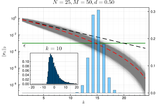
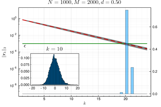
Figure 1. The CGA applied to $W\bm{x}=\bm{f}_{1}$ were $W\overset{\mathscr{L}}{=}\mathcal{W}_{\beta}(N,M)$, $N/M\xrightarrow[]{M\to\infty}d$. The dashed black curve indicates the large $M$ limit for the error $\|\bm{r}_{k}\|_{2}$ at step $k$ and the dashed red curve gives $\mathbb{E}\|\bm{r}_{k}\|_{2}$ at step $k$. The shaded gray area is an ensemble of 10000 runs of the method, displaying the norms that resulted. The overlaid histogram shows the rescaled fluctuations in the error at $k=10$. As $M\to\infty$ this approaches a Gaussian density. Lastly, the histogram in the main frame gives the halting distribution for $\epsilon=0.001$ (green line). It is highly concentrated when $N=1000,M=2000$. With these parameters, Remark 2 implies that for $M$ large, the algorithm will run for approximately $\left\lceil 2\frac{\log\epsilon}{\log d}\right\rceil=20$ iterations.

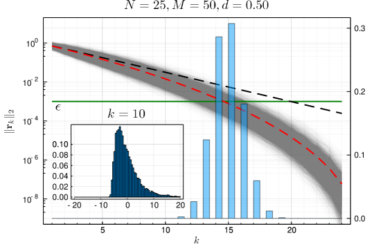
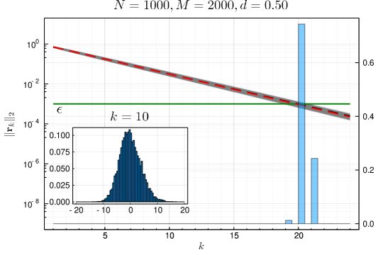
Figure 2. The CGA applied to $W\bm{x}=M^{-1}XX^{*}\bm{x}=f_{1}$ were $X$ has iid entries with $\mathbb{P}(X_{ij}=0)=2/3,\mathbb{P}(X_{ij}=\pm\sqrt{3})=1/6$. The black dashed curve indicates the large $M$ limit for the error $\|\bm{r}_{k}\|_{2}$ at step $k$ the dashed red curve gives $\mathbb{E}\|\bm{r}_{k}\|_{2}$ at step $k$ in the case of $W\overset{\mathscr{L}}{=}\mathcal{W}_{\beta}(N,M)$, for comparison. The shaded gray area is an ensemble of 10000 runs of the method, displaying the errors that resulted. The overlaid histogram shows the rescaled fluctuations in the error at $k=10$. As $M\to\infty$ this approaches a Gaussian density. Lastly, the histogram in the main frame gives the halting distribution for $\epsilon=0.001$ (green line). With these parameters, Remark 2 implies that for $M$ large, the algorithm will run for approximately $\left\lceil 2\frac{\log\epsilon}{\log d}\right\rceil=20$ iterations.

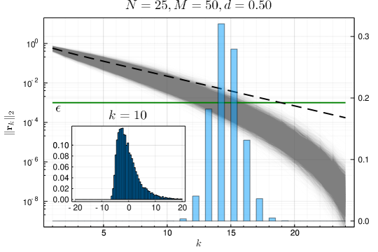
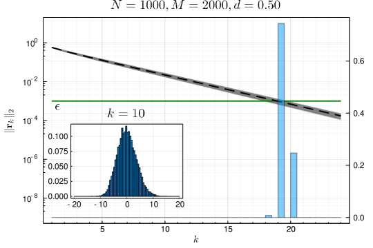
Figure 3. The MINRES algorithm applied to $W\bm{x}=\bm{f}_{1}$ were $W\overset{\mathscr{L}}{=}\mathcal{W}_{\beta}(N,M).$ The dashed curve indicates the large $M$ limit for the error $\|\bm{r}_{k}\|_{2}$ at step $k$. The shaded gray area is an ensemble of 10000 runs of the method, displaying the errors that resulted. The overlaid histogram shows the rescaled fluctuations in the error at $k=10$. As $M\to\infty$ this approaches a Gaussian density. Lastly, the histogram in the main frame gives the halting distribution for $\epsilon=0.001$ (green line). With these parameters, Remark 3 implies that for $M$ large, the algorithm will run for approximately $\left\lceil\frac{\log\frac{\epsilon^{2}}{1-d+\epsilon^{2}d}}{\log d}\right\rceil=19$ iterations.

Figure 4. The MINRES algorithm applied to $W\bm{x}=M^{-1}XX^{*}\bm{x}=f_{1}$ were $X$ has iid entries with $\mathbb{P}(X_{ij}=0)=2/3,\mathbb{P}(X_{ij}=\pm\sqrt{3})=1/6$. The shaded gray area is an ensemble of 10000 runs of the method, displaying the errors that resulted. The overlaid histogram shows the rescaled fluctuations in the error at $k=10$. As $M\to\infty$ this approaches a Gaussian density. Lastly, the histogram in the main frame gives the halting distribution for $\epsilon=0.001$ (green line). With these parameters, Remark 3 implies that for $M$ large, the algorithm will run for approximately $\left\lceil\frac{\log\frac{\epsilon^{2}}{1-d+\epsilon^{2}d}}{\log d}\right\rceil=19$ iterations.

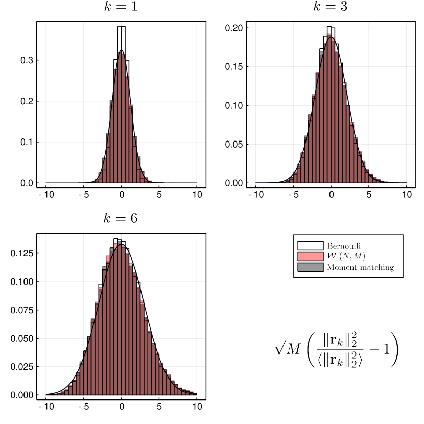
Figure 5. A comparison of the rescaled statistics (9) across three distributions. Since the Bernoulli ensemble fails to match the moments in (6), we see that it does not match the variance (7).

$k$	$k/2(1+1/d)$	Wishart	Moment matching	Bernoulli
1	1.5	1.493	1.48	1.003
2	3.0	3.002	2.997	2.511
3	4.5	4.532	4.519	4.036
4	6.0	6.040	6.039	5.527
5	7.5	7.576	7.54	7.004
6	9.0	9.135	9.054	8.547

Table 1. A numerical demonstration of the necessity of the moment matching condition (6). This table gives the sample variance of (9) across three different distributions for $N=500,d=1/2$ and 50,000 samples.

2. Sample covariance matrices and classical numerical linear algebra

A fundamental property of a matrix $X\overset{\mathscr{L}}{=}\mathcal{G}_{\beta}(N,M)$ is its orthogonal ($\beta=1$) or unitary ($\beta=2$) invariance. That is, let $Q$ be an $N\times N$ fixed orthogonal matrix then

$$QWQ^{*}\overset{\mathscr{L}}{=}W,\quad W=XX^{*}.$$

If $\beta=2$, then $Q$ can be a complex unitary matrix. Furthermore, this is true even if $Q$ is random, provided it is independent of $X$.

Let $W\overset{\mathscr{L}}{=}\mathcal{W}_{\beta}(N,M)$ and perform an eigenvalue decomposition $W=U\Lambda U^{*}$, $U^{*}U=I$. It follows directly from the invariance of the Wishart distribution that the vector

$$\bm{\omega}=\begin{bmatrix}|U_{11}|^{2}\\ \vdots\\ |U_{1n}|^{2}\end{bmatrix},\quad\text{ where }\quad\left[U_{ij}\right]_{1\leq i,j\leq n}=U$$

can be parameterized by

(10) $$\bm{\omega}\overset{\mathscr{L}}{=}\frac{\bm{\nu}}{\|\bm{\nu}\|}_{1},$$

where $\bm{\nu}$ is a vector of iid $\chi_{\beta}^{2}$ random variables. This fact is discussed in detail in [DT19, Appendix A].

2.0.1. The eigenvalues of the Wishart distributions

The global asymptotic eigenvalue distribution of the Wishart distributions is the same, regardless of the choice of $\beta=1,2$. The classical setup is the following. For $W\overset{\mathscr{L}}{=}\mathcal{W}_{\beta}(N,M)$, define the (random) empirical spectral measure

$$\mu_{\mathrm{em}}(\mathrm{d}\lambda;W)=\frac{1}{N}\sum_{j=1}^{N}\delta_{\lambda_{j}(W)}(\mathrm{d}\lambda).$$

Recall the parameter $\mathfrak{d}=N/M$.

Definition 1.

Define the Marchenko–Pastur law for all $d>0$ by

(11) $$\varrho_{d}(\mathrm{d}x)=\frac{1}{2\pi d}\sqrt{\frac{[(x-\gamma_{-})(\gamma_{+}-x)]_{+}}{x^{2}}}\mathrm{d}x+\left[1-\frac{1}{d}\right]_{+}\delta_{0}(\mathrm{d}x),\quad\text{where}\quad\gamma_{\pm}=(1\pm\sqrt{d})^{2}$$

are the spectral edges. The notation $[\cdot]_{+}$ refers to the positive part of $(\cdot).$

The following gives the global eigenvalue distribution (see [BS10], for example):

Theorem 2.1.

Suppose that $\mathfrak{d}\xrightarrow[]{M\to\infty}d\in(0,1]$. Then

$$\mu_{\mathrm{em}}(\mathrm{d}\lambda;\mathcal{W}_{\beta}(N,M))\xrightarrow[N\to\infty]{(d)}\varrho_{d}(\mathrm{d}\lambda),$$

almost surely.

Historically, the behavior of individual eigenvalues, and gaps between eigenvalues, have been studied extensively. In the analysis we present it is not necessary to use such detailed microscopic results. Instead, we need finer results about global properties of the matrix. One such example is the so-called central limit theorem for linear statistics.

The Bai-Silverstein [BS04] central limit theorem for linear statistics of sample covariance matrices shows that for sufficiently smooth functions $f,$

$$\sum_{j=1}^{N}f(\lambda_{j})-N\int f(x)\varrho_{\mathfrak{d}}(\mathrm{d}x)=N\int f(x)(\mu_{\mathrm{em}}(\mathrm{d}x)-\varrho_{\mathfrak{d}}(\mathrm{d}x))\xrightarrow[N\to\infty]{(d)}\mathcal{N}_{1}(\mu_{f},\sigma_{f}^{2}).$$

The standard deviation $\sigma_{f}$ can be understood as a weighted Sobolev-1/2 norm of $f$, restricted to the support of the Marchenko-Pastur law. Other related central limit theorems for linear spectral statistics of sample covariance matrices include [DE06, Shc11, Joh98].

But the classical central limit theorem for linear statistics involves the empirical spectral measure $\mu_{\mathrm{em}}(\mathrm{d}\lambda;W)$ which rarely arises in a numerical or computational context. What is much more likely to arise is the weighted empirical spectral measure: for $\bm{b}\in\mathbb{C}^{N}$, $\|\bm{b}\|_{2}=1$ and $W=W^{*}\in\mathbb{C}^{N\times N}$ the weighted empirical spectral measure is given by

(12) $$\mu=\mu_{\bm{b}}=\sum_{j=1}^{N}\omega_{j}\delta_{\lambda_{j}},\quad(\omega_{j})_{j=1}^{N}=|U^{*}\bm{b}|^{2},\quad W=U\Lambda U^{*},\quad U^{*}U=I,\quad\Lambda=\mathrm{diag}(\lambda_{1},\ldots,\lambda_{N}).$$

We refer to this as the spectral measure associated to the pair $(W,\bm{b})$.

We show in Section 5 that for polynomials $p$ and a sample covariance matrix $W$ with identity covariance and for which $\mathfrak{d}\to d,$

$$\sqrt{M}\int f(x)(\mu_{\bm{b}}(\mathrm{d}x)-\varrho_{\mathfrak{d}}(dx))\xrightarrow[N\to\infty]{(d)}\mathcal{N}_{1}(0,\widehat{\sigma_{f}}^{2}).$$

Note that the rate of the central limit theorem changes dramatically from the case of the central limit theorem for linear statistics. Although we will not need it, the variance $\widehat{\sigma_{f}}^{2}$ can be expressed as $c_{\beta,d}\int f^{2}(x)\varrho_{d}(dx)$. Similar theorems have been proven before, most notably by [ORS14] who prove a more general statement in the case that $\bm{b}$ is a coordinate vector. There is also [ORS13] in which the analogous statement is made for Wigner matrices. We also mention [Duy18] and [DS15] which prove related theorems for Gaussian cases.

While it is natural to assume these statements extend to other classes of test functions beyond polynomials, we will not need them (except for the specific case of $f(x)=1/x,$ which we handle by other means – note that the extension to analytic functions in a neighborhood of the Marchenko-Pastur law does not need new ideas beyond what is necessary for the polynomial case)

2.1. Sample covariance matrices with independence

In the current work, we use a restricted definition of a sample covariance matrix.

Definition 2.

A real ($\beta=1$) or complex ($\beta=2$) sample covariance matrix is given by $W\overset{\mathscr{L}}{=}XX^{*}$ where $X$ is an $N\times M$ random matrix with independent entries satisfying

$$\mathbb{E}X_{ij} =0,~{}~{}~{}\mathbb{E}(\Re X_{ij})(\Im X_{ij})=0,~{}~{}~{}\mathbb{E}(\Re X_{ij})^{2}=\frac{1}{\beta M},$$

$$\mathbb{E}|X_{ij}|^{2} =\frac{1}{M},\quad\text{and}\quad\mathbb{E}|\sqrt{M}X_{ij}|^{p}\leq C_{p},\quad\text{for all }p\in\mathbb{N}.$$

In some cases, we will need restrictions on the first four generalized moments.

Definition 3.

A sample covariance matrix satisfies the $\beta=1,2$ moment matching condition if

$$\mathbb{E}(\Re X_{ij})^{\ell}(\Im X_{ij})^{p}=\mathbb{E}(\Re Y)^{\ell}(\Im Y)^{p}$$

where $Y\overset{\mathscr{L}}{=}\mathcal{N}_{\beta}(0,1/M)$, for all choices of non-negative integers $\ell,p$ such that $\ell+p\leq 4$.

Remark 9.

To see the necessity of the moment matching condition consider a sample covariance matrix $W^{\prime}=XX/M$ where $X^{\prime}$ is $N\times M,$ with $X^{\prime}_{ij}=\pm 1$ with equal probability and $W\overset{\mathscr{L}}{=}\mathcal{W}_{1}(N,M)$. Then consider the first moments of the spectral measures $\mu$ and $\mu^{\prime}$ associated to $(W,\bm{f}_{1})$ and $(W^{\prime},\bm{f}_{1})$, respectively:

$$\int\lambda\mu(\mathrm{d}\lambda) =\frac{1}{M}\bm{f}_{1}^{T}XX^{T}\bm{f}_{1}\overset{\mathscr{L}}{=}\frac{\chi_{M}^{2}}{M},$$

$$\int\lambda\mu^{\prime}(\mathrm{d}\lambda) =\frac{1}{M}\bm{f}_{1}^{T}X^{\prime}X^{\prime T}\bm{f}_{1}=1.$$

2.2. The Golub–Kahan bidiagonalization algorithm

Definition 4.

A Jacobi matrix is given by

$$T=\begin{bmatrix}a_{0}&b_{0}\\ b_{0}&a_{1}&b_{1}\\ &b_{1}&a_{2}&\ddots\\ &&\ddots&\ddots\end{bmatrix}.$$

It may be finite or semi-infinite. The entries are real and $b_{j}>0$ for $j\geq 0$.

A reduction of $W=XX^{*}$ to a Jacobi matrix can be obtained via the Golub–Kahan bidiagonalization procedure. The distributional action of this algorithm on the Wishart ensembles $\mathcal{W}_{\beta}(N,M)$ is given in [DE02]. Specifically, if $W=M^{-1}XX^{*}\overset{\mathscr{L}}{=}\mathcal{W}_{\beta}(N,M)$, $X\overset{\mathscr{L}}{=}\mathcal{G}_{\beta}(N,M)$ then there exists unitary matrices $U_{1}$, $U_{2}$ such that

(13) $$\begin{split}U_{1}XU_{2}&\overset{\mathscr{L}}{=}\sqrt{\beta}X_{\mathrm{GK}},\\ \sqrt{\beta}X_{\mathrm{GK}}&\overset{\mathscr{L}}{=}\left[\begin{array}[]{ccccc|cccccc}\chi_{\beta M}&&&&&\\ \chi_{\beta(N-1)}&\chi_{\beta(M-1)}&&&&\\ &\chi_{\beta(N-2)}&\chi_{\beta(M-2)}&&&&0&\\ &&\ddots&\ddots&&\\ &&&\chi_{\beta}&\chi_{\beta(M-N+1)}\end{array}\right],\end{split}$$

where all entries are independent. Therefore the law of the entries of the tridiagonal matrix $U_{1}WU_{1}^{*}=M^{-1}U_{1}XU_{2}U_{2}^{*}X^{*}U_{1}^{*}=\beta X_{\mathrm{GK}}X_{\mathrm{GK}}^{T}$ is completely parameterized.

2.3. The Lanczos iteration

The Lanczos iteration is another algorithm for obtaining a tridiagonal reduction of a matrix.

Algorithm 1: Lanczos Iteration (1) $\bm{q}_{1}$ is the initial vector. Suppose $\|\bm{q}_{1}\|_{2}^{2}=\bm{q}_{1}^{*}\bm{q}_{1}=1$, $W^{*}=W$. (2) Set $b_{-1}=1$, $\bm{q}_{0}=0.$ (3) For $k=1,2,\ldots,n$ (a) Compute $\displaystyle a_{k-1}=(W\bm{q}_{k}-b_{k-2}\bm{q}_{k-1})^{*}\bm{q}_{k}$. (b) Set $\bm{v}_{k}=W\bm{q}_{k}-a_{k-1}\bm{q}_{k}-b_{k-2}\bm{q}_{k-1}$. (c) Compute $b_{k-1}=\|\bm{v}_{k}\|_{2}$ and if $b_{k-1}\neq 0$, set $\bm{q}_{k+1}=\bm{v}_{k}/b_{k-1}$, otherwise terminate.

The Lanczos algorithm at step $k\leq N$ produces a matrix $T_{k}$ and orthogonal vectors $\bm{q}_{1},\ldots,\bm{q}_{k}$

$$Q_{k}=\begin{bmatrix}\bm{q}_{1}&\bm{q}_{2}&\cdots&\bm{q}_{k}\end{bmatrix},\quad T_{k}=T_{k}(W,\bm{y}_{1})=\begin{bmatrix}a_{0}&b_{0}\\ b_{0}&a_{1}&\ddots\\ &\ddots&\ddots&b_{k-2}\\ &&b_{k-2}&a_{k-1}\end{bmatrix},$$

such that

(14) $$WQ_{k}=Q_{k}T_{k}+b_{k-1}\bm{q}_{k+1}\bm{f}_{k}^{*}$$

We use the notation $T=T(W,\bm{q}_{1})=T_{n}(W,\bm{q}_{1})$ for the matrix produced when the Lanczos iteration is run for its maximum of $n$ steps.

The following is entirely classical [TBI97].

Lemma 2.2.

Suppose $W$ is a symmetric matrix. And suppose that the Lanczos iteration does not terminate before step $n\leq N$. For $k=1,2,\ldots,n$,

$$\bm{q}_{1},\ldots,\bm{q}_{k}$$

is an orthonormal basis for the Krylov subspace $\mathcal{K}_{k}=\mathrm{span}\{\bm{q}_{1},W\bm{q}_{1},\ldots,W^{k-1}\bm{q}_{1}\}.$

The following result gives us the distribution of $T_{k}$ throughout the Lanczos iteration applied to a Wishart matrix and it is a direct consequence of the invariance of the Wishart distributions.

Theorem 2.3.

Suppose $W\overset{\mathscr{L}}{=}\mathcal{W}_{\beta}(N,M)$. For any given $\bm{q}_{1}\in\mathbb{R}^{n}$ with $\|\bm{q}_{1}\|_{2}=1$(or $\mathbb{C}^{n}$ for $\beta=2$) with probability one, the Lanczos iteration does not terminate if $k<n:=\min\{N,M\}$. And the distribution on $a_{k},b_{k}$, $k=0,2,\ldots,n-1$ does not depend on $\bm{q}_{1}$. In a distributional sense it suffices to take $\bm{q}_{1}=\bm{f}_{1}$ and therefore the distribution is determined by the Householder tridiagonalization of $W$, i.e., the Golub–Kahan bidiagonalization of $X$.

Every $N\times N$ symmetric tridiagonal matrix $T$ produces a probability measure

$$\mu_{T}=\sum_{j=1}^{N}\omega_{j}\delta_{\lambda_{j}}$$

where $\lambda_{j}$’s are the eigenvalues of $T$ and $\omega_{j}$ is the squared modulus of the first component of the normalized eigenvector associated to $\lambda_{j}$. The spectral measure $\mu_{T}$, $T=T(W,\bm{b})$ coincides with the spectral measure associated to the pair $(W,\bm{b})$ whenever $\bm{b}$ is a unit vector. There is a bijection between such measures and Jacobi matrices [Dei00].

3. Theory of orthogonal polynomials

Let $\mu$ be a Borel probability measure on $\mathbb{R}$ with finite moments. The orthonormal polynomials $(p_{n})_{n\geq 0}$, $p_{n}(\lambda)=p_{n}(\lambda;\mu)$ are constructed by applying the Gram–Schmidt process to the sequence of functions

$$\{\lambda\mapsto 1,\lambda\mapsto\lambda,\lambda\mapsto\lambda^{2},\ldots\}.$$

If the support of $\mu$ contains at least $N$ points then one is guaranteed to be able to construct $(p_{0},p_{1},\ldots,p_{N-1})$.

3.1. Hankel determinants, moments and the three-term recurrence

We now recall the classical fact that the coefficients in a three-term recurrence relation can be recovered as an algebraic function of the moments of the associated spectral measure. For a given sequence of orthonormal polynomials, $(p_{j}(\lambda))_{j\geq 0}=(p_{j}(x;\mu))_{j\geq 0}$ with respect to a measure $\mu$, we have the associated three-term recurrence

(15) $$\lambda p_{n}(\lambda)=b_{n}p_{n+1}(\lambda)+a_{n}p_{n}(\lambda)+b_{n-1}p_{n-1}(\lambda),\quad n\geq 0,\quad b_{n}>0,$$

with the convention $p_{-1}(\lambda)=0$ and $b_{-1}=0$. Here $b_{n}=b_{n}(\mu),a_{n}=a_{n}(\mu)$ are called the recurrence coefficients. We will use the following proposition in a critical way to translate any discussion of the output of the Lanczos iteration to a discussion of orthogonal polynomials.

Proposition 3.1.

The three-term recurrence coefficients generated by the spectral measure associated to the pair $(W,\bm{b})$, $W>0,\|\bm{b}\|_{2}=1$ coincide with the entries of the Lanczos matrix $T(W,\bm{b})$.

We write $p_{n}(\lambda)=\ell_{n}\lambda^{n}+s_{n}\lambda^{j-1}+\cdots$ and find by equating coefficients that

$$\ell_{n}=b_{n}\ell_{n+1},$$

$$a_{n}\ell_{n}=b_{n}s_{n+1}.$$

Define $D_{n}$ and $D_{n}(\lambda)$ by the determinants

$$D_{n} =\det M_{n},\quad(M_{n})_{ij}=m_{i+j-2},\quad 1\leq i,j\leq n+1,\quad m_{j}(\mu)=m_{j}=\int\lambda^{j}\mu(\mathrm{d}\lambda),$$

$$D_{n}(\lambda) =\det M_{n}(\lambda),$$

and $M_{n}(\lambda)$ is formed by replacing the last row of $M_{n}$ with the row vector $[1~{}\lambda~{}\lambda^{2}\cdots\lambda^{n}]$. Then, it is well-known that [Dei00]

$$p_{n}(\lambda)=\frac{D_{n}(\lambda)}{\sqrt{D_{n}D_{n-1}}},$$

and therefore

(16) $$\ell_{n}=\sqrt{\frac{D_{n-1}}{D_{n}}},\quad s_{n}=\det\tilde{M}_{n},$$

where $\tilde{M}_{n}$ is the matrix formed by removing the last row and second-to-last column of $M_{n}$. This shows that $a_{n}/\sqrt{D_{n-1}}$ and $b^{2}_{n}$ are rational functions of determinants of matrices involving only the moments of $\mu$ up to order $2n$.

Associated to the three-term recurrence (15) is the Jacobi matrix

$$T=\begin{bmatrix}a_{0}&b_{0}\\ b_{0}&a_{1}&b_{1}\\ &b_{1}&a_{2}&\ddots\\ &&\ddots&\ddots\end{bmatrix}.$$

Let $T_{n}$ denote the upper-left $n\times n$ subblock of $T$. It follows immediately that $T_{n}$ is a differentiable function of $(m_{0},m_{1},\ldots,m_{2n})$ on the open subset of $\mathbb{R}^{2n+1}$ where all $D_{k}>0$ for $1\leq k\leq n$. We also note that

(17) $$\bm{f}_{1}^{*}T^{k}\bm{f}_{1}=\int\lambda^{k}\mu(\mathrm{d}\lambda).$$

This can be seen by a direct calculation if $T$ is a finite-dimensional matrix. If $T$ is semi-infinite, then this fact follows from [Dei00, (2.25)].

3.2. Monic polynomials and Stieltjes transforms

The monic orthogonal polynomials associated to a measure $\mu$ are given by

(18) $$\pi_{n}(\lambda;\mu)=\pi_{n}(\lambda) =p_{n}(\lambda)/\ell_{n}=\lambda^{n}+\cdots.$$

We will also need the Stieltjes transform of the monic polynomials

(19) $$c_{n}(z;\mu)=c_{n}(z) =\int_{\mathbb{R}}\frac{\pi_{n}(\lambda)}{\lambda-z}\mu(\mathrm{d}\lambda).$$

With the convention that $b_{0}=1$, $\pi_{-1}\equiv 0$ and $c_{-1}\equiv-1$ it is elementary that the following recurrences are satisfied for $n=0,1,2,\ldots,$

$$\pi_{n+1}(\lambda)=(\lambda-a_{n})\pi_{n}(\lambda)-b_{n-1}^{2}\pi_{n-1}(\lambda),\quad\pi_{0}(\lambda)=1,$$

$$c_{n+1}(z)=(z-a_{n})c_{n}(z)-b_{n-1}^{2}c_{n-1}(z),\quad c_{0}(z)=\int_{\mathbb{R}}\frac{\mu(\mathrm{d}\lambda)}{\lambda-z}.$$

4. The conjugate gradient algorithm and the MINRES algorithm

In this section we discuss three algorithms: the CGA, the CGA applied to the normal equations and the MINRES algorithm.

4.1. The CGA

The actual CGA is given by the following.

Algorithm 2: Conjugate Gradient Algorithm (1) $\bm{x}_{0}$ is the initial guess. (2) Set $\bm{r}_{0}=\bm{b}-W\bm{x}_{0}$, $\bm{p}_{0}=\bm{r}_{0}$. (3) For $k=1,2,\ldots,n$ (a) Compute $\displaystyle a_{k-1}=\frac{\bm{r}_{k-1}^{*}\bm{r}_{k-1}}{\bm{r}_{k-1}^{*}W\bm{p}_{k-1}}$. (b) Set $\bm{x}_{k}=\bm{x}_{k-1}+a_{k-1}\bm{p}_{k-1}$. (c) Set $\bm{r}_{k}=\bm{r}_{k-1}-a_{k-1}W\bm{p}_{k-1}$. (d) Compute $\displaystyle b_{k-1}=-\frac{\bm{r}_{k}^{*}\bm{r}_{k}}{\bm{r}_{k-1}^{*}\bm{r}_{k-1}}$. (e) Set $\bm{p}_{k}=\bm{r}_{k}-b_{k-1}\bm{p}_{k-1}$.

As noted previously, a remarkable fact is that the iterates $\bm{x}_{k}$ of the CGA applied to the linear system $W\bm{x}=\bm{b}$ are given by the solution of the minimization problem (4) [HS52]. From this, we see that $\bm{y}\in\mathcal{K}_{k}$ can be written as

$$\bm{y}=\sum_{j=0}^{k-1}c_{j}W^{j}\bm{b}\quad\Rightarrow\quad\bm{x}-\bm{y}=W^{-1}\left(\bm{b}-\sum_{j=0}^{k-1}c_{j}W^{j+1}\bm{b}\right)=W^{-1}q_{\bm{y}}(W)\bm{b},$$

for a polynomial $q_{\bm{y}}$ of degree at most $k$ and it satisfies $q_{\bm{y}}(0)=1$. Then, computing further,

$$\|\bm{x}-\bm{y}\|_{W}^{2}=\bm{b}^{*}q_{\bm{y}}(W)^{*}W^{-1}q_{\bm{y}}(W)\bm{b}.$$

And setting $W=U\Lambda U^{*}$, we find

$$\|\bm{x}-\bm{y}\|_{W}^{2}=\sum_{j=1}^{N}\frac{|q_{\bm{y}}(\lambda_{j})|^{2}}{\lambda_{j}}|(U^{*}\bm{b})_{j}|^{2}=\int\frac{|q_{\bm{y}}(\lambda)|^{2}}{\lambda}\mu_{T}(\mathrm{d}\lambda),\quad T=T(W,\bm{b}).$$

Now, all directional derivatives of this, when $\bm{y}=\bm{x}_{k}$, with respect to coefficients of the polynomial must vanish identically. This gives a characterization of $q_{\bm{x}_{k}}$: Let $\delta q_{k}$ be a polynomial of degree at most $k$ that satisfies $\delta q_{k}(0)=0$ and we must have

$$0=\int q_{\bm{x}_{k}}(\lambda)\frac{\delta q_{k}(\lambda)}{\lambda}\mu_{T}(\mathrm{d}\lambda).$$

This implies that $q_{\bm{x}_{k}}(\lambda)$ is orthogonal to all lower-degree polynomials, with respect to $\mu_{T}$: It is given by

$$q_{\bm{x}_{k}}(\lambda)=\frac{\pi_{k}(\lambda;\mu_{T})}{\pi_{k}(0;\mu_{T})}.$$

Proposition 4.1.

Let $\bm{x}_{k}$ be the computed solution at step $k$ of the CGA applied to $W\bm{x}=\bm{b}$. For any $k\in\mathbb{N}$, with $T=T(W,\bm{b})$,

$$\|\bm{e}_{k}\|_{W}^{2}=\frac{c_{k}(0;\mu_{T})}{\pi_{k}(0;\mu_{T})}\quad\text{and}\quad\|\bm{r}_{k}\|^{2}_{2}=\frac{\prod_{j=0}^{k-1}b_{j}(\mu_{T})^{2}}{\pi_{k}(0;\mu_{T})^{2}}.$$

Proof.

By orthogonality

$$\|\bm{e}_{k}\|_{W}^{2} =\int_{\mathbb{R}}\frac{\pi_{k}(\lambda;\mu_{T})^{2}}{\lambda\pi_{k}(0;\mu_{T})^{2}}\mu_{T}(d\lambda)$$

$$=\int_{\mathbb{R}}\frac{\pi_{k}(\lambda;\mu_{T})\left(\pi_{k}(0;\mu_{T})\lambda^{-1}+\sum_{j=1}^{k}c_{j}\lambda^{k-1}\right)}{\pi_{k}(0;\mu_{T})^{2}}\mu_{T}(d\lambda)=\int_{\mathbb{R}}\frac{\pi_{k}(\lambda;\mu_{T})}{\lambda\pi_{k}(0;\mu_{T})}\mu_{T}(d\lambda)$$

$$=\frac{c_{k}(0;\mu_{T})}{\pi_{k}(0;\mu_{T})}.$$

For the $\bm{r}_{k}$ equation, by definition of the polynomials $\{p_{n}\}$, we have that

(20) $$\int_{\mathbb{R}}{\pi_{k}(\lambda;\mu_{T})^{2}}\mu_{T}(d\lambda)=\frac{1}{\ell_{k}^{2}}\int_{\mathbb{R}}{p_{k}(\lambda;\mu_{T})^{2}}\mu_{T}(d\lambda)=\frac{1}{\ell_{k}^{2}}=\prod_{j=0}^{k-1}b_{j}(\mu_{T})^{2}.$$

∎

4.2. MINRES

The MINRES algorithm, at iteration $k$ gives the solution of

$$\bm{x}_{k}=\mathrm{argmin}_{\bm{y}\in\mathcal{K}_{k}}\|\bm{b}-W\bm{y}\|_{2}.$$

More explicitly, the algorithm is given by:

Algorithm 3: MINRES Algorithm for $W\bm{x}=\bm{b}$ (1) Suppose $W=W^{*}\in\mathbb{C}^{N\times N}$, $\epsilon>0.$ (2) Set $\bm{q}_{1}=\bm{b}/\|\bm{b}\|_{2}.$ (3) For $k=1,2,\ldots,n$, $n\leq N$ (a) Compute $\displaystyle a_{k-1}=(W\bm{q}_{k}-b_{k-2}\bm{q}_{k-1})^{*}\bm{q}_{k}$. (b) Set $\bm{v}_{k}=W\bm{q}_{k}-a_{k-1}\bm{q}_{k}-b_{k-2}\bm{q}_{k-1}$. (c) Compute $b_{k-1}=\|\bm{v}_{k}\|_{2}$ and if $b_{k-1}\neq 0$, set $\bm{q}_{k+1}=\bm{v}_{k}/b_{k-1}$. (d) Form $\displaystyle\tilde{T}_{k}=\begin{bmatrix}a_{0}&b_{0}\\ b_{0}&a_{1}&\ddots\\ &\ddots&\ddots&b_{k-2}\\ &&b_{k-2}&a_{k-1}\\ &&&b_{k-1}\end{bmatrix}.$ (e) Compute $\bm{z}_{k}=\mathrm{argmin}_{\bm{z}\in\mathbb{C}^{k}}\|\tilde{T}_{k}\bm{z}-\|\bm{b}\|_{2}\bm{f}_{1}\|_{2}.$ (f) If $\|\tilde{T}_{k}\bm{z}_{k}-\|\bm{b}\|_{2}\bm{f}_{1}\|_{2}<\epsilon$, return $\bm{x}_{k}=\begin{bmatrix}\bm{q}_{1}&\cdots&\bm{q}_{k}\end{bmatrix}\bm{z}_{k}$.

Following the same prescription as in the previous section we are led to the problem of finding the polynomial $r_{\bm{x}_{k}}$ of degree less than or equal to $k$ satisfying $r_{\bm{x}_{k}}(0)=1$ that minimizes

$$\|\bm{b}-W\bm{y}\|_{2}^{2}=\sum_{j=1}^{N}|r_{\bm{y}}(\lambda_{j})|^{2}|(U^{*}\bm{b})_{j}|^{2}=\int|r_{\bm{y}}(\lambda)|^{2}\mu_{T}(\mathrm{d}\lambda),\quad T=T(W,\bm{b}),$$

among all such polynomials. We then must have

$$0=\int r_{\bm{x}_{k}}(\lambda)\delta r_{k}(\lambda)\mu_{T}(\mathrm{d}\lambda)$$

for all polynomials $\delta r_{k}$ of degree less than or equal to $k$ with $\delta r_{k}(0)=0$. So, write $r_{x_{k}}(\lambda)=\sum_{j=0}^{k}c_{j}p_{j}(\lambda;\mu_{T})$. And choosing $\delta r_{k}(\lambda)=p_{\ell}(\lambda;\mu_{T})-p_{\ell}(0;\mu_{T})$ we find

$$0=\int\left(\sum_{j=0}^{k}c_{j}p_{j}(\lambda;\mu_{T})\right)\left(p_{\ell}(\lambda;\mu_{T})-p_{\ell}(0;\mu_{T})\right)\mu_{T}(\mathrm{d}\lambda)\Leftrightarrow c_{\ell}=p_{\ell}(0;\mu_{T})c_{0}.$$

From this, we obtain

(21) $$r_{\bm{x}_{k}}(\lambda;\mu_{T})=\frac{\sum_{j=0}^{k}p_{j}(0;\mu_{T})p_{j}(\lambda;\mu_{T})}{\sum_{j=0}^{k}p_{j}^{2}(0;\mu_{T})}.$$

Proposition 4.2.

Let $\bm{x}_{k}$ be the computed solution at step $k$ of the MINRES algorithm applied to $W\bm{x}=\bm{b}$. For any $k\in\mathbb{N}$, with $T=T(W,\bm{b})$

$$\|\bm{r}_{k}\|_{2}^{2} =\frac{1}{\sum_{j=0}^{k}p_{j}^{2}(0;\mu_{T})}$$

$$=\frac{1}{b_{k}(\mu_{T})^{2}\left[p_{k+1}^{\prime}(0;\mu_{T})p_{k}(0;\mu_{T})-p_{k}^{\prime}(0;\mu_{T})p_{k+1}(0;\mu_{T})\right]},$$

$$=\frac{\prod_{j=0}^{k-1}b_{j}(\mu_{T})^{2}}{\pi_{k+1}^{\prime}(0)\pi_{k}(0;\mu_{T})-\pi_{k}^{\prime}(0;\mu_{T})\pi_{k+1}(0;\mu_{T})}$$

Proof.

Integrating (21)

$$\|\bm{b}-W\bm{x}_{k}\|_{2}^{2}=\frac{1}{\sum_{j=0}^{k}p_{j}^{2}(0;\mu_{T})}.$$

Employing the Christoffel-Darboux formula,

$$\sum_{j=0}^{k}p_{j}^{2}(0;\mu_{T}) =\frac{\ell_{k}}{\ell_{k+1}}\left[p_{k+1}^{\prime}(0;\mu_{T})p_{k}(0;\mu_{T})-p_{k}^{\prime}(0;\mu_{T})p_{k+1}(0;\mu_{T})\right]$$

$$=b_{k}(\mu_{T})^{2}\left[p_{k+1}^{\prime}(0;\mu_{T})p_{k}(0;\mu_{T})-p_{k}^{\prime}(0;\mu_{T})p_{k+1}(0;\mu_{T})\right].$$

Then using (20)

$$p_{k}(\lambda;\mu_{T})=\left(\prod_{j=0}^{k-1}b_{j}(\mu_{T})^{-1}\right)\pi_{k}(\lambda;\mu_{T})$$

we find the alternate expression

$$\sum_{j=0}^{k}p_{j}^{2}(0;\mu_{T})=\left(\prod_{j=0}^{k-1}b_{j}(\mu_{T})^{-2}\right)\left[\pi_{k+1}^{\prime}(0;\mu_{T})\pi_{k}(0;\mu_{T})-\pi_{k}^{\prime}(0;\mu_{T})\pi_{k+1}(0;\mu_{T})\right].$$

∎

4.3. The CGA on the normal equations

Next, for $X\in\mathbb{C}^{N\times M}$, $N\leq M$, consider solving the normal equations $XX^{*}\bm{x}=X\bm{b}$ with the CGA. The appearance of $X$ on the right-hand side changes the minimization problem one has to consider. With $W=XX^{*}$, the CGA will solve

$$\bm{x}_{k}=\mathrm{argmin}_{\bm{y}\in\mathcal{K}_{k}}\|\bm{x}-\bm{y}\|_{W},\quad\mathcal{K}_{k}= \{X\bm{b},WX\bm{b},\ldots,W^{k-1}X\bm{b}\}.$$

As before, we express

$$\bm{x}-\bm{y}=W^{-1}q_{\bm{y}}(W)X\bm{b}.$$

Using the singular value decomposition $X=U\Sigma V^{*}$ where $U,V$ are square matrices, we write

$$\|\bm{x}-\bm{y}\|_{W}^{2} =\bm{b}^{*}V\Sigma^{*}U^{*}q_{\bm{y}}(W)^{*}W^{-1}q_{\bm{y}}(W)U\Sigma V^{*}\bm{b},$$

$$=\bm{b}^{*}V\Sigma^{*}q_{\bm{y}}(\Lambda)^{*}\Lambda^{-1}q_{\bm{y}}(\Lambda)\Sigma V^{*}\bm{b}$$

where $\Lambda=\Sigma\Sigma^{*}$. Since $\Sigma$ has its last $M-N$ columns being identically zero, we use the notation $\Sigma=\begin{bmatrix}\Sigma_{0}&0\end{bmatrix}$ and find $\Lambda=\Sigma_{0}^{2}.$ Thus

$$\|\bm{x}-\bm{y}\|_{W}^{2}=\bm{c}^{*}\Sigma_{0}q_{\bm{y}}(\Lambda)^{*}\Lambda^{-1}q_{\bm{y}}(\Lambda)\Sigma_{0}\bm{c},\quad\bm{c}=\begin{bmatrix}I&0\end{bmatrix}V^{*}\bm{b}.$$

The techniques used in the case of MINRES directly apply.

Proposition 4.3.

Let $\bm{x}_{k}$ be the computed solution at step $k$ of applying the CGA to the normal equations $XX^{*}\bm{x}=X\bm{b}$, $X\in\mathbb{C}^{N\times M}$, $N\leq M$. For any $k\in\mathbb{N}$,

$$\|\bm{e}_{k}\|_{W}^{2} =\frac{\prod_{j=0}^{k-1}b_{j}(\nu)^{2}}{\pi_{k+1}^{\prime}(0;\nu)\pi_{k}(0;\nu)-\pi_{k}^{\prime}(0;\nu)\pi_{k+1}(0;\nu)}=\frac{1}{\sum_{j=0}^{k}p_{j}^{2}(0;\nu)},$$

where

(22) $$\nu=\sum_{j=1}^{N}\omega_{j}\delta_{\lambda_{j}},\quad\omega_{j}=|(V^{*}\bm{b})_{j}|^{2},$$

$X=U\Sigma V^{*}$ is the singular value decomposition of $X$ and $\lambda_{1},\ldots,\lambda_{N}$ are the eigenvalues of $XX^{*}$.

5. Universality

5.1. Bidiagonal central limit theorem, Gaussian case

Throughout the asymptotic analysis that follows $d$ will be a fixed positive real number and $\mathfrak{d}=N/M\xrightarrow[]{M\to\infty}d$. Taking the entrywise limit in (13), using the notation

$$\frac{1}{\sqrt{\beta M}}X_{\mathrm{GK}} =\begin{bmatrix}H&0\end{bmatrix},$$

(28) $$H \overset{\mathscr{L}}{=}\frac{1}{\beta M}\left[\begin{array}[]{ccccc}\chi_{\beta M}\\ \chi_{\beta(N-1)}&\chi_{\beta(M-1)}\\ &\chi_{\beta(N-2)}&\chi_{\beta(M-2)}\\ &&\ddots&\ddots\\ &&&\chi_{\beta}&\chi_{\beta(M-N+1)}\end{array}\right],$$

it follows that

$$H\xrightarrow[N\to\infty]{(d)}\mathbb{H}_{d}=\begin{bmatrix}1&\\ \sqrt{d}&1\\ &\sqrt{d}&1\\ &&\ddots&\ddots\end{bmatrix}.$$

This limit is in the sense of weak convergence of the finite-dimensional marginals of a random infinite bidiagonal matrix.

Furthermore, for a $\chi_{k}$ random variable

$${\chi_{k}}-\sqrt{k}\xrightarrow[k\to\infty]{(d)}\mathcal{N}_{1}(0,1/2),$$

and so by independence, for iid standard normals $\{Z_{j}\}_{1}^{\infty},$

(29) $$\sqrt{2\beta M}(H-\mathbb{H}_{\mathfrak{d}})\xrightarrow[N\to\infty]{(d)}\mathbb{G}=\begin{bmatrix}Z_{1}&\\ Z_{2}&Z_{3}\\ &Z_{4}&Z_{5}\\ &&\ddots&\ddots\end{bmatrix}.$$

From here, it follows immediately that the Jacobi matrix produced by the Lanczos algorithm applied to $\mathcal{W}_{\beta}(N,M)$ has a limit, in the same sense of finite-dimensional marginal convergence, to an infinite tridiagonal matrix.

Definition 5.

Given a positive-definite Jacobi matrix $T$ we define $\varphi$ to be the function that gives the Cholesky factorization of $T$. That is $\varphi(T)=H$ where $H$ is a lower-triangular bidiagonal matrix with all non-negative entries and $HH^{*}=T$.

The Cholesky factorization $\varphi(T)$ is unique for $T>0$ and $\varphi$ is generically differentiable (see [ER05]). The actual algorithm to compute it is given as follows:

Algorithm 4: Jacobi matrix Cholesky factorization (1) Suppose $T$ is an $N\times N$ positive-definite Jacobi matrix, set $H=T.$ (2) For $k=1,2,\ldots,N-1$ (a) Set $H_{k+1,k+1}=H_{k+1,k+1}-\displaystyle\frac{H_{k+1,k}^{2}}{H_{kk}}.$ (b) Set $H_{k:k+1,k}=H_{k:k+1,k}/\sqrt{H_{k,k}}.$ (3) Set $H_{N,N}=\sqrt{H_{N,N}}.$ (4) Return $\varphi(T)=H.$

The following is immediate.

Proposition 5.1.

Let $W\overset{\mathscr{L}}{=}\mathcal{W}_{\beta}(N,M)$, $N\leq M$. For any sequence of unit vectors $\bm{b}=\bm{b}_{N}$ of length $N,$

$$\sqrt{2\beta M}(\varphi(T(W,\bm{b}_{N}))-\mathbb{H}_{\mathfrak{d}})\xrightarrow[N\to\infty]{(d)}\mathbb{G}.$$

Now, define

$$\mathbb{H}_{d}\mathbb{H}_{d}^{*}=\mathbb{T}_{d}:=\begin{bmatrix}1&\sqrt{d}\\ \sqrt{d}&1+d&\sqrt{d}\\ &\sqrt{d}&1+d&\ddots&\\ &&\ddots&\ddots\end{bmatrix}.$$

Proposition 5.2.

Let $W\overset{\mathscr{L}}{=}\mathcal{W}_{\beta}(N,M)$ for $N\leq M$ where $\mathfrak{d}\xrightarrow[]{M\to\infty}d\in(0,1]$. Then for any sequence of unit vectors $\bm{b}=\bm{b}_{N}$ of length $N,$ with $T=T(W,\bm{b}),$ the vector

$$\left(\sqrt{\beta M}\bm{f}_{1}^{*}(T^{k}-\mathbb{T}_{\mathfrak{d}}^{k})\bm{f}_{1}\right)_{k\geq 1}=\left(\sqrt{\beta M}\int_{\mathbb{R}}x^{k}(\mu_{T}(\mathrm{d}x)-\varrho_{\mathfrak{d}}(\mathrm{d}x))\right)_{k\geq 1},$$

converges in the sense of finite-dimensional marginals to a centered Gaussian random vector $\mathcal{G}=(G_{1})_{k\geq 1}$.

Proof.

The equality follows using (17). The proposition then follows using (29) because, for each $k$, $\sqrt{M}\bm{f}_{1}^{*}(T^{k}-\mathbb{T}_{\mathfrak{d}}^{k})\bm{f}_{1}$ depends only on a finite number of elements of $T$. ∎

5.2. Contour integral reformulation of the moments

Let $\Gamma$ be a simple curve that encloses the nonzero spectrum of a symmetric tridiagonal matrix $T$. Then

$$m_{k}(\mu_{T})=\frac{1}{2\pi i}\oint_{\Gamma}z^{k}c_{0}(z;\mu_{T})\mathrm{d}z.$$

Now, let $\Gamma=\Gamma_{d}$ be a smooth simple contour that properly encloses the support of the Marchenko–Pastur law (11).

We denote the Stieltjes transform $s_{d}(z)$ of (11) by

(30) $$s_{d}(z)=\int_{\mathbb{R}}\frac{\varrho_{d}(\mathrm{d}\lambda)}{\lambda-z}.$$

There are many classical references for the following result.

Theorem 5.3 (Global eigenvalue bounds, see, e.g. [DS01, Gem80, Sil85, Ver09]).

For the eigenvalues $\lambda_{N}\leq\cdots\leq\lambda_{1}$ of $W\overset{\mathscr{L}}{=}\mathcal{W}_{\beta}(N,M)$, $N\leq M$ and $t>0$

$$\mathbb{P}\left(1-\sqrt{\frac{N}{M}}-t\leq\lambda_{N}^{1/2}\leq\lambda_{1}^{1/2}\leq 1+\sqrt{\frac{N}{M}}+t\right)\xrightarrow[]{M\to\infty}0.$$

Hence with probability tending to $1$ as $M\to\infty$, $\mathfrak{d}\xrightarrow[]{M\to\infty}d$, the support of $\mu_{T}$, $T=T(W,\bm{b})$ is contained within $\Gamma_{d}$. As a corollary, we have:

Corollary 5.4.

Let $W\overset{\mathscr{L}}{=}\mathcal{W}_{\beta}(N,M)$ for $N\leq M$ where $\mathfrak{d}\xrightarrow[]{M\to\infty}d\in(0,1]$. Then for any sequence of unit vectors $\bm{b}=\bm{b}_{N}$ of dimension $N,$ with $T=T(W,\bm{b}),$ the vector

$$\left(\frac{\sqrt{M}}{2\pi i}\oint_{\Gamma_{d}}z^{k}(c_{0}(z;\mu_{T})-s_{\mathfrak{d}}(z))\mathrm{d}z\right)_{k\geq 1}\xrightarrow[N\to\infty]{(d)}\mathcal{G},$$

in the sense of finite-dimensional marginals, where $\mathcal{G}$ is the same process as in Proposition 5.2.

We also need to treat the case of $k=-1$. Suppose $T=HH^{T}$ where $H$ is real, square, lower-triangular and given by

(31) $$H=\begin{bmatrix}\alpha_{0}\\ \beta_{0}&\alpha_{1}\\ &\beta_{1}&\alpha_{2}\\ &&\ddots&\ddots\end{bmatrix}$$

Then $T_{11}=\alpha_{0}^{2}$ and $T_{jj}=\alpha_{j-1}^{2}+\beta_{j-2}^{2}$ for $j>1$. Let $\tilde{H}$ be the matrix formed by removing the first row and column of $H$ and let $\tilde{T}=\tilde{H}\tilde{H}^{T}$. Then it follows by Cramer’s rule that

(32) $$\bm{f}_{1}^{*}T^{-1}\bm{f}_{1}=\frac{\det(\beta_{0}^{2}\bm{f}_{1}\bm{f}_{1}^{*}+\tilde{T})}{\det T}=\frac{(\det\tilde{T})(1+\beta_{0}^{2}\bm{f}_{1}^{*}\tilde{T}^{-1}\bm{f}_{1})}{\det T}=\frac{1}{\alpha_{0}^{2}}(1+\beta_{0}^{2}\bm{f}_{1}^{*}\tilde{T}^{-1}\bm{f}_{1}).$$

From this expression, one obtains

$$\bm{f}_{1}^{*}T^{-1}\bm{f}_{1}=\frac{1}{\alpha_{0}^{2}}\left(1+\sum_{j=1}^{N-1}\prod_{k=1}^{j}\left(\frac{\beta_{k-1}^{2}}{\alpha_{k}^{2}}\right)\right).$$

Following [Mui82, Theorem 3.2.12]:

Proposition 5.5.

Let $\bm{y}$ be random vector in $\mathbb{C}^{N}$ that does not vanish a.s. Let $X$ be an $N\times M$ matrix with independent $\mathcal{N}_{\beta}(0,1)$ entries independent of $\bm{y}.$ Then

$$\frac{\bm{y}^{*}\bm{y}}{\bm{y}(XX^{*})^{-1}\bm{y}}\overset{\mathscr{L}}{=}\beta^{-1}\chi_{\beta(M-N+1)}^{2}$$

and therefore

$$\bm{f}_{1}^{*}T^{-1}\bm{f}_{1}\overset{\mathscr{L}}{=}\frac{\beta M}{\chi_{\beta(M-N+1)}^{2}}.$$

Proof.

The first claim can be established using the QR factorization of $X$. The second claim for $\bm{f}_{1}^{*}T^{-1}\bm{f}_{1}$ follows from the first once we realize $T=T(M^{-1}XX^{*},\bm{b}),$ then $\bm{f}_{1}^{*}T^{-1}\bm{f}_{1}=M\bm{b}^{*}(XX^{*})^{-1}\bm{b}$. ∎

As we can also apply the same proposition to an $(N-1)\times(M-1)$ matrix of normals, and conclude

$$\bm{f}_{1}^{*}\tilde{T}^{-1}\bm{f}_{1}\overset{\mathscr{L}}{=}\frac{\beta M}{\chi_{\beta(M-N+1)}^{2}}.$$

Using (32) this provides a remarkable identity in law involving chi-square distributions:

Proposition 5.6.

For any integers $\ell\geq 0$ and $M\geq N\geq 1$

$$\frac{\beta M}{\chi^{2}_{\beta(M-N+1)}}\overset{\mathscr{L}}{=}\frac{1}{\chi_{\beta(M-\ell)}^{2}}\left(1+\chi_{\beta(N-\ell-1)}^{2}\frac{\beta M}{\chi_{\beta(M-N+1)}^{2}}\right)$$

where the chi-squared variables on the right-hand side are mutually independent.

But more importantly, iterating (32) $\ell$ times and applying and using Proposition 5.5 to describe the remainder, we have:

Proposition 5.7.

Suppose $H$ is distributed as in (28). Then for $0<\ell<N$

$$\bm{f}_{1}^{*}T^{-1}\bm{f}_{1}=\frac{1}{\alpha_{0}^{2}}\left(1+\sum_{j=1}^{\ell}\prod_{k=1}^{j}\frac{\beta_{k-1}^{2}}{\alpha_{k}^{2}}+\left(\beta_{\ell}^{2}\frac{\beta M}{\chi_{\beta(M-N+1)}^{2}}\right)\prod_{k=1}^{\ell}\frac{\beta_{k-1}^{2}}{\alpha_{k}^{2}}\right)$$

where $\chi_{\beta(M-N+1)}$ depends only on $H_{\ell+1:N,\ell+1:N}$.

The following notation is convenient.

Definition 6.

We write $X_{M}=c_{M}+Y_{M}+o(M^{-1/2})$ if

$$\sqrt{M}(X_{M}-c_{M}),\quad\text{and}\quad\sqrt{M}(Y_{M}),$$

converge, in distribution, to the same distribution as $M\to\infty$.

Let $\ell$ be fixed. We use the approximation in distribution (29), $\alpha_{j}=1+Z_{2j+1}/\sqrt{2\beta M}+o(M^{-1/2})$, $\beta_{j}=\sqrt{\mathfrak{d}}+Z_{2j+2}/\sqrt{2\beta M}+o(M^{-1/2})$ to find

(33) $$\alpha_{j}^{2} =1+\frac{\sqrt{2}}{\sqrt{\beta M}}Z_{2j+1}+o(M^{-1/2}),$$

(34) $$\beta_{j}^{2} =\mathfrak{d}+\frac{\sqrt{2\mathfrak{d}}}{\sqrt{\beta M}}Z_{2j+2}+o(M^{-1/2}),$$

$$\frac{\beta M}{\chi_{\beta(M-N+1)}^{2}} =\frac{1}{1-\mathfrak{d}}\left(1+\frac{\sqrt{2}}{\sqrt{1-\mathfrak{d}}\sqrt{\beta M}}Z_{0}\right)+o(M^{-1/2}),\quad Z_{0}\overset{\mathscr{L}}{=}\mathcal{N}_{1}(0,1),$$

and compute as $N\to\infty$

$$1+ \sum_{j=1}^{\ell}\prod_{k=1}^{j}\left(\frac{\beta_{k-1}^{2}}{\alpha_{k}^{2}}\right)=1+\sum_{j=1}^{\ell}\prod_{k=1}^{j}\mathfrak{d}\left[1+\frac{\sqrt{2}}{\sqrt{\beta M}}\left(Z_{2k}/\sqrt{d}-Z_{2k+1}\right)\right]$$

$$=\frac{1-\mathfrak{d}^{\ell+1}}{1-\mathfrak{d}}+\frac{\sqrt{2}}{\sqrt{\beta M}}\sum_{k=1}^{\ell}\mathfrak{d}^{k}\frac{1-\mathfrak{d}^{\ell-k+1}}{1-\mathfrak{d}}\left(Z_{2k}/\sqrt{\mathfrak{d}}-Z_{2k+1}\right)+o(M^{-1/2}).$$

Thus

$$\sqrt{\beta M}\left(\bm{f}_{1}^{*}T^{-1}\bm{f}_{1}-\frac{1}{1-\mathfrak{d}}\right)\xrightarrow[M\to\infty]{(d)}\sqrt{2}\frac{Z_{1}}{d-1}+\sqrt{2}\sum_{k=1}^{\infty}\frac{d^{k}}{1-d}(Z_{2k}/\sqrt{d}-Z_{2k+1}).$$

We arrive at the following proposition.

Proposition 5.8.

Suppose $H$ is distributed as in (28) where the entries are labelled according to (31) and $T=HH^{*}$. Let $\mathcal{Z}=[Z_{1},Z_{2},\ldots]^{T}$ be a vector of iid standard normal random variables. Then if $N\leq M,\mathfrak{d}\xrightarrow[]{M\to\infty}d\in(0,1)$

$$\sqrt{\beta M} \left(\bm{f}_{1}^{*}T^{-1}\bm{f}_{1}-\frac{1}{1-\mathfrak{d}}\right)\xrightarrow[M\to\infty]{(d)}Z_{-1},$$

$$Z_{-1} :=-\sqrt{2}\frac{Z_{1}}{1-d}+\sqrt{2}\sum_{k=1}^{\infty}\frac{d^{k}}{1-d}(Z_{2k}/\sqrt{d}-Z_{2k+1}).$$

Additionally,

$$\sqrt{\beta M}\left(\begin{bmatrix}\bm{f}_{1}^{*}T^{-1}\bm{f}_{1}\\ \alpha_{0}\\ \beta_{0}\\ \alpha_{1}\\ \beta_{1}\\ \vdots\end{bmatrix}-\begin{bmatrix}\frac{1}{1-\mathfrak{d}}\\ 1\\ \sqrt{\mathfrak{d}}\\ 1\\ \sqrt{\mathfrak{d}}\\ \vdots\end{bmatrix}\right)\xrightarrow[M\to\infty]{(d)}\begin{bmatrix}Z_{-1}\\ \mathcal{Z}/\sqrt{2}\end{bmatrix}$$

in the sense of convergence of finite-dimensional marginals.

5.3. Universality for the moment fluctuations of the spectral measure

We now generalize Corollary 5.4 to general distributions. Let $R(z)=R(z;X)=(XX^{*}-z\operatorname{Id})^{-1}$ denote the resolvent of $XX^{*}$ and define $G(z)=G(z;X)=\begin{bmatrix}-I&X^{*}\\ X&-zI\end{bmatrix}^{-1}$. The following is a direct consequence of [KY17, Theorems 3.6 and 3.7].

Proposition 5.9.

Suppose $X$ is a sample covariance matrix with $\mathfrak{d}=N/M\xrightarrow[]{M\to\infty}d\in(0,\infty)$. For any $\delta,\epsilon>0$ and for any $R,D>0$ there is a constant $C$ so that for all $M\in\mathbb{N},$

$$\sup_{z\in\Gamma} \sup_{\bm{v},\bm{w}\in\mathbb{C}^{N+M}}\mathbb{P}\left[\left|\bm{v}^{*}G(z)\bm{w}-\bm{v}^{*}\Pi_{\mathfrak{d}}(z)\bm{w}\right|\geq\|\bm{v}\|\|\bm{w}\|M^{\epsilon-1/2}\right]\leq CM^{-D},$$

$$\quad\Pi_{\mathfrak{d}}(z) =\begin{bmatrix}-(1+s_{\mathfrak{d}}(z))^{-1}I_{M}&0\\ 0&s_{\mathfrak{d}}(z)I_{N}\end{bmatrix},$$

and therefore

$$\sup_{z\in\Gamma}\sup_{\bm{v},\bm{w}\in\mathbb{C}^{N}}\mathbb{P}\left[\left|\bm{v}^{*}R(z)\bm{w}-s_{\mathfrak{d}}(z)\bm{v}^{*}\bm{w}\right|\geq\|\bm{v}\|\|\bm{w}\|M^{\epsilon-1/2}\right]\leq CM^{-D},$$

where $\Gamma$ is any bounded simple closed curve that does not intersect the support of $\varrho_{d}$.

Define the classical eigenvalue locations $\gamma_{i}=\gamma_{i}^{(N)}$ by $N\int_{\gamma_{i}}^{\infty}\varrho_{\mathfrak{d}}(\mathrm{d}x)=i-1/2$ and from [KY17, Theorem 3.12] we have:

Proposition 5.10 (Eigenvalue rigidity).

Let $X$ be a sample covariance matrix and denote the eigenvalues of $XX^{*}$ by $\lambda_{1}\geq\lambda_{2}\geq\cdots\geq\lambda_{N}$. For any $\epsilon>0$ and for any $D>0$ there is a constant $C$ so that

$$\mathbb{P}\left(|\lambda_{i}-\gamma_{i}|>N^{\epsilon}(\max\{i,N+1-i\})^{-1/3}N^{-2/3}~{}~{}\text{for any}~{}~{}i\right)\leq CN^{-D}.$$

Definition 7.

Let $\Phi:\mathbb{C}^{n}\to\mathbb{R}$ be bounded. Suppose, in addition, that for any multi-index $\alpha=(\alpha_{1},\ldots,\alpha_{n})$, $1\leq|\alpha|\leq 5$ and for any $\epsilon^{\prime}>0$ sufficiently small, we have

$$\max\{|\partial^{\alpha}\Phi(x_{1},\ldots,x_{n})|:\max_{j}|x_{j}| \leq M^{\epsilon^{\prime}}\}\leq M^{C_{0}\epsilon^{\prime}},$$

for $C_{0}>0$. Then $\Phi$ is called an admissible test function.

Theorem 5.11 (Comparison).

Let $W=XX^{*}$ and $\tilde{W}=YY^{*}$ be two sample covariance matrices such that

$$\mathbb{E}(\Re X_{ij})^{\ell}(\Im X_{ij})^{p}=\mathbb{E}(\Re Y_{ij})^{\ell}(\Im Y_{ij})^{p},\quad\ell+p\leq 4,\quad 1\leq i\leq N,\quad 1\leq j\leq M.$$

For each $j$, let $\Gamma_{j}=\partial\Omega_{j}$, $\Omega_{j}=\overline{\Omega}_{j}$ be a simple smooth positively-oriented curve that is uniformly bounded away from support of the Marchenko–Pastur law $\varrho_{d}$. Suppose that $f_{1},f_{2},\ldots,f_{n}$ is a finite collection of functions that are analytic in a neighborhood of $\Omega$. Then for any admissible test function $\Phi:\mathbb{C}^{n}\to\mathbb{R}$ we have for $T=T(W,\bm{b}),\tilde{T}=T(\tilde{W},\bm{b}),$

$$\left|\mathbb{E}\Phi\left(\frac{\sqrt{M}}{2\pi i}\oint_{\Gamma_{1}}f_{1}(z)(c_{0}(z;\mu_{T})-s_{\mathfrak{d}}(z))\mathrm{d}z,\ldots,\frac{\sqrt{M}}{2\pi i}\oint_{\Gamma_{n}}f_{n}(z)(c_{0}(z;\mu_{T})-s_{\mathfrak{d}}(z))\mathrm{d}z\right)\right.$$

$$-\left.\mathbb{E}\Phi\left(\frac{\sqrt{M}}{2\pi i}\oint_{\Gamma_{1}}f_{1}(z)(c_{0}(z;\mu_{\tilde{T}})-s_{\mathfrak{d}}(z))\mathrm{d}z,\ldots,\frac{\sqrt{M}}{2\pi i}\oint_{\Gamma_{n}}f_{n}(z)(c_{0}(z;\mu_{\tilde{T}})-s_{\mathfrak{d}}(z))\mathrm{d}z\right)\right|$$

$$\leq CM^{-\sigma}$$

for some $C,\sigma>0$. Here $C$ will depend on $n$, the constants $C_{p}$ in Definition 2, $\Phi$, $\Gamma_{1},\ldots,\Gamma_{n}$ and $f_{1},\ldots,f_{n}$ and $\sigma$ will depend on the constant $C_{0}$ in Definition 7.

Remark 10.

Note that in Theorem 5.11, if $\mathfrak{d}$ is bounded uniformly away from one, a contour $\Gamma_{j}$ could just encircle $z=0$. And if $\mathfrak{d}\to d\in(0,1]$ the only non-trivial case is where the contour $\Gamma_{j}$ encircles the entire support of $\varrho_{d}$.

This gives immediate corollaries.

Corollary 5.12.

Suppose $W$ is a sample covariance matrix satisfying the moment matching condition (Definition 3) with $\mathfrak{d}=N/M\xrightarrow[]{M\to\infty}d\in(0,\infty)$. Then for any sequence of unit vectors $\bm{b}=\bm{b}_{N}$ of length $N,$ with $T=T(W,\bm{b}),$ the vector

$$\left(\frac{\sqrt{M}}{2\pi i}\oint_{\Gamma}z^{k}(c_{0}(z;\mu_{T})-s_{\mathfrak{d}}(z))\mathrm{d}z\right)_{k\geq 1}\xrightarrow[N\to\infty]{(d)}\mathcal{G},$$

in the sense of finite-dimensional marginals, where $\mathcal{G}$ is the same process as in Proposition 5.2.

Corollary 5.13.

Suppose $W$ is a sample covariance matrix satisfying the moment matching condition (Definition 3) with $\mathfrak{d}=N/M\xrightarrow[]{M\to\infty}d\in(0,\infty)$. Then for any sequence of unit vectors $\bm{b}=\bm{b}_{N}$ of length $N,$ with $T=T(W,\bm{b})$, let $H$ be given by the Cholesky factorization of of $T$, $H=\varphi(T)$ and label the entries of $H$ as in (31). Then Proposition 5.8 holds for $H$.

Proof.

Fix $k$. For all $N>k,$ the Hankel matrix of moments $(m_{j+r-2}(\mu_{T}))_{j,r=1}^{k}$ is positive definite almost surely. On this set, the mapping to $(m_{j}(\mu_{T}):0\leq j\leq 2k)\mapsto T_{k}(W,\bm{b})$ is differentiable. It follows that $H_{k}$, the upper-left $k\times k$ subblock of $H$ is also a differentiable function $m_{j}(\mu_{T})$, $j=0,1,\ldots,2k$. Then the corollary follows directly from Theorem 5.11. ∎

Before we prove Theorem 5.11, we establish some intermediate results.

Lemma 5.14.

For an $N\times M$ matrix $X$ and $\Im z\neq 0$

(35) $$\begin{bmatrix}-I&X^{*}\\ X&-zI\end{bmatrix}^{-1} =\begin{bmatrix}(z^{-1}XX^{*}-I)^{-1}&(X^{*}X-zI)^{-1}X^{*}\\ X(X^{*}X-zI)^{-1}&(XX^{*}-zI)^{-1},\\ \end{bmatrix}$$

(36) $$\left\|\begin{bmatrix}-I&X^{*}\\ X&-zI\end{bmatrix}^{-1}\right\| \leq(|z|+1)|\Im z|^{-1}+2\sqrt{|\Im z|^{-1}+|z||\Im z|^{-2}}$$

Recall that $\bm{f}_{1},\bm{f}_{2},\ldots$ denotes the standard basis and we use the notation $\hat{\bm{u}}=\begin{bmatrix}0\\ \bm{u}\end{bmatrix}\in\mathbb{C}^{N+M}$ for $\bm{u}\in\mathbb{C}^{N}$.

Lemma 5.15 (Resolvent expansion with leading-order correction).

Let $X$ be an iid matrix satisfying the assumptions of Definition 2. Let $Q$ be the matrix that is equal to $X$ with the exception of one entry that is set to zero so that $X=Q+X_{ij}\bm{f}_{i}\bm{f}_{j}^{*}$ for some $1\leq i\leq N,1\leq j\leq M$. For two unit vectors $\bm{u},\bm{v}\in\mathbb{C}^{N}$

$$\hat{\bm{u}}^{*}S(z;X)\hat{\bm{v}} =\hat{\bm{u}}^{*}S(z;Q)\hat{\bm{v}}+\sum_{k=1}^{3}M^{-k/2}J_{k}+M^{-5/2}J_{4},$$

$$S(z;X) =\sqrt{M}\left[G(z;X)-\Pi_{d}(z)\right],$$

and for every $\epsilon>0$ and $D>0$ there exists $C>0$ such that $J_{4}$ satisfies

$$\mathbb{P}(|J_{4}|>M^{\epsilon})\leq CM^{-D}.$$

In addition, $J_{k}$ for $k<4$ is a finite sum of the form

$$J_{k}=\sum_{\ell}f_{k,\ell}g_{k,\ell},$$

where $g_{k,\ell}$ is a monomial in $X_{ij}\sqrt{M}$ and $\overline{X_{ij}}\sqrt{M}$ with degree at most $k+1$ and $f_{k,\ell}$ is independent of $X_{ij}$ satisfying that for every $\epsilon>0$ and $D>0$ there exists $C>0$ such that

$$\mathbb{P}(|f_{k,\ell}|>M^{\epsilon})\leq CM^{-D}.$$

Proof.

Write $V:=X_{ij}\bm{f}_{i+M}\bm{f}_{j}^{*}+\overline{X_{ij}}\bm{f}_{j}\bm{f}_{i+M}^{*}$. Consider for a diagonal matrix $D$

$$\hat{\bm{u}}^{*}DVD\hat{\bm{v}} =X_{ij}(\hat{\bm{u}}^{*}D\bm{f}_{i+M})(\bm{f}_{j}^{*}D\hat{\bm{v}})+\overline{X_{ij}}(\hat{\bm{u}}^{*}D\bm{f}_{j})(\bm{f}_{i+M}^{*}D\hat{\bm{v}})$$

(37) $$=X_{ij}(\hat{\bm{u}}^{*}D_{i+M,i+M}\bm{f}_{i+M})(\bm{f}_{j}^{*}D_{jj}\hat{\bm{v}})+\overline{X_{ij}}(\hat{\bm{u}}^{*}D_{jj}\bm{f}_{j})(\bm{f}_{i+M}^{*}D_{i+M,i+M}\hat{\bm{v}})=0.$$

This is because $1\leq j\leq M$ and $\hat{\bm{u}},\hat{\bm{v}}$ must have zeros in their first $M$ entries.

We then consider the expansion of

$$S(z;X) =S(z;Q)-\sqrt{M}G(z;Q)VG(z;Q)+\cdots$$

$$+\sqrt{M}[G(z;Q)V]^{4}G(z;Q)$$

$$-\sqrt{M}[G(z;Q)V]^{5}G(z;X).$$

We write

$$\hat{\bm{u}}^{*} \sqrt{M}G(z;Q)VG(z;Q)\hat{\bm{v}}=\sqrt{M}\hat{\bm{u}}^{*}\Pi_{d}(z)V\Pi_{d}(z)\hat{\bm{v}}+E_{ij}.$$

From (37) the first term vanishes. Explicitly,

$$E_{ij} =\hat{\bm{u}}^{*}\left[S(z;Q)VG(z;Q)+G(z;Q)VS(z;Q)+M^{-1/2}S(z;Q)VS(z;Q)\right]\hat{\bm{v}},$$

$$=X_{ij}(\hat{\bm{u}}^{*}S(z;Q)\bm{f}_{j+M})(\bm{f}_{i}^{*}G(z,Q)\hat{\bm{v}})+\overline{X_{ij}}(\hat{\bm{u}}^{*}G(z;Q)\bm{f}_{i})(\bm{f}_{j+M}^{*}S(z,Q)\hat{\bm{v}})$$

$$+X_{ij}(\hat{\bm{u}}^{*}G(z;Q)\bm{f}_{j+M})(\bm{f}_{i}^{*}S(z,Q)\hat{\bm{v}})+\overline{X_{ij}}(\hat{\bm{u}}^{*}S(z;Q)\bm{f}_{i})(\bm{f}_{j+M}^{*}G(z,Q)\hat{\bm{v}})$$

$$+M^{-1/2}X_{ij}(\hat{\bm{u}}^{*}S(z;Q)\bm{f}_{j+M})(\bm{f}_{i}^{*}S(z,Q)\hat{\bm{v}})+M^{-1/2}\overline{X_{ij}}(\hat{\bm{u}}^{*}S(z;Q)\bm{f}_{i})(\bm{f}_{j+M}^{*}S(z,Q)\hat{\bm{v}}).$$

Observe that this is a linear function of $X_{ij},\overline{X_{ij}}$ with coefficients that are independent of $X_{ij}$ and controlled by Proposition 5.9.

Then consider

$$\hat{\bm{u}}^{*}(G(z;Q)V)^{j}G(z;Q)\hat{\bm{v}}.$$

With the notation $a_{1}=X_{ij},a_{2}=\overline{X_{ij}}$, $\bm{v}_{1}=\bm{f}_{j+M},\bm{v}_{2}=\bm{f}_{i}$, and $\bm{w}_{1}=\bm{f}_{i},\bm{w}_{2}=\bm{f}_{j+M}$ one has for $\ell=2,3,4$

$$\sqrt{M}\hat{\bm{u}}^{*}(G(z;Q)V)^{\ell}G(z;Q)\hat{\bm{v}}$$

$$=\sqrt{M}\sum_{p\in\{1,2\}^{\ell}}\left[\left(\prod_{k=1}^{\ell}a_{p_{k}}\right)(\hat{\bm{u}}^{*}G(z;Q)\bm{v}_{p_{1}})(\bm{w}_{p_{\ell}}^{*}G(z;Q)\hat{\bm{v}})\prod_{k=1}^{\ell-1}(\bm{w}_{p_{k}}^{*}G(z;Q)\bm{v}_{p_{k+1}})\right]:=P^{(\ell)}_{ij}$$

and set

$$P^{(5)}_{ij}:=\sqrt{M}\sum_{p\in\{1,2\}^{5}}\left[\left(\prod_{k=1}^{5}a_{p_{k}}\right)(\hat{\bm{u}}^{*}G(z;Q)\bm{v}_{p_{1}})(\bm{w}_{p_{\ell}}^{*}G(z;X)\hat{\bm{v}})\prod_{k=1}^{4}(\bm{w}_{p_{k}}^{*}G(z;Q)\bm{v}_{p_{k+1}})\right].$$

Whenever two vectors are orthogonal because they have disjoint support, we can replace $G(z)$ with $S(z)/\sqrt{M}$. When $\ell$ is odd, suppose that for a choice of $p\in\{1,2\}^{\ell}$ no two vectors are orthogonal in such a way. Then $p_{1}=1$ so that $\hat{\bm{u}}$ is not orthogonal to $\bm{v}_{p_{1}}$. And then $\bm{w}_{i}$ and $\bm{v}_{j}$ are not orthogonal if $i\neq j$, so then $p_{2}=2$, $p_{3}=1$, and so on. This implies that $p_{\ell}=1$ because $\ell$ is odd. But then $\hat{\bm{v}}$ is orthogonal to $\bm{v}_{p_{\ell}}$. This implies that the order of the odd terms is actually one less than is immediately apparent. Write

$$\hat{\bm{u}}^{*}S(z;X)\hat{\bm{v}} =\hat{\bm{u}}^{*}S(z;Q)\hat{\bm{v}}+\sum_{k=1}^{3}M^{-k/2}J_{k}+M^{-5/2}J_{4}=\hat{\bm{u}}^{*}S(z;Q)\hat{\bm{v}}+\xi,$$

$$J_{1} =M^{1/2}(E_{ij}+P_{ij}^{(2)}),\quad J_{2}=MP_{ij}^{(3)},$$

$$J_{3} =M^{3/2}P_{ij}^{(4)},\quad J_{4}=M^{5/2}P_{ij}^{(5)}.$$

∎

Proposition 5.16 (Green’s function replacement).

Suppose $\Phi$ is an admissible test function. Suppose further that $X$ and $Y$ are two matrices satisfying assumptions in Definition 2 and that

$$\mathbb{E}X_{ij}^{\ell}\overline{X_{ij}}^{p}=\mathbb{E}Y_{ij}^{\ell}\overline{Y_{ij}}^{p},$$

for all choices of $\ell,p\in\mathbb{N}$, $\ell+p\leq 4$ and $1\leq i\leq N,1\leq j\leq M$. Then for any $\epsilon>0$, any families of unit vectors $\{\bm{q}_{j}\}_{j=1}^{n}$, $\{\bm{p}_{j}\}_{j=1}^{n}$, and any collection of points $\{z_{j}\}_{j=1}^{n}$ bounded uniformly away from the support of the Marchenko–Pastur law $\varrho_{d}$ and bounded away from the real axis by $M^{-\delta}$, $1>\delta>0$ we have

$$\left|\mathbb{E}\Phi(\hat{\bm{q}}_{1}^{*}S(z_{1},X)\hat{\bm{p}}_{1},\ldots,\hat{\bm{q}}_{n}^{*}S(z_{n},X)\hat{\bm{p}}_{n})-\mathbb{E}\Phi(\hat{\bm{q}}_{1}^{*}S(z_{1},Y)\hat{\bm{p}}_{1},\ldots,\hat{\bm{q}}_{n}^{*}S(z_{n},Y)\hat{\bm{p}}_{n})\right|\leq Cn^{5}M^{-1/2+C^{\prime}\epsilon},$$

where $C^{\prime}>0$ depends only $C_{0}$ in Definition 7.

Proof.

The following proof is adapted from [EY17, Theorem 16.1] and [KY17]. Let $\phi:\llbracket 1,MN\rrbracket\to\llbracket 1,N\rrbracket\times\llbracket 1,M\rrbracket$ be a bijection. For $\gamma\in\llbracket 1,MN\rrbracket$ define $X_{\gamma}$ by

$$(X_{\gamma})_{\phi(\ell)}=\begin{cases}Y_{\phi(\ell)}&\ell\leq\gamma,\\ X_{\phi(\ell)}&\ell>\gamma.\end{cases}$$

Note that $X_{0}=X$ and $X_{MN}=Y$ and that $X_{\gamma}$ and $X_{\gamma+1}$ differ only in the $\phi(\gamma+1)$ entry. Define $Q_{\gamma}$ by $(Q_{\gamma})_{\phi(\ell)}=(X_{\gamma+1})_{\phi(\ell)}$ if $\ell\neq\gamma+1$ and $(Q_{\gamma})_{\phi(\gamma+1)}=0$, so that $Q_{\gamma}$ has a zero in the exact entry where $X_{\gamma}$ and $X_{\gamma+1}$ differ. We then compare $X_{\gamma}$ to $Q_{\gamma}$ using Lemma 5.15 and a fifth-order Taylor expansion of $\Phi$

$$\Phi(\hat{\bm{q}}_{1}^{*}S(z_{1},X_{\gamma})\hat{\bm{p}}_{1},\ldots,\hat{\bm{q}}_{n}^{*}S(z_{n},X_{\gamma})\hat{\bm{p}}_{n})$$

$$=\Phi(\hat{\bm{q}}_{1}^{*}S(z_{1},Q_{\gamma})\hat{\bm{p}}_{1}+\xi_{1},\ldots,\hat{\bm{q}}_{n}^{*}S(z_{n},Q_{\gamma})\hat{\bm{p}}_{n}+\xi_{n})$$

$$=\Phi(\hat{\bm{q}}_{1}^{*}S(z_{1},Q_{\gamma})\hat{\bm{p}}_{1},\ldots,\hat{\bm{q}}_{n}^{*}S(z_{n},Q_{\gamma})\hat{\bm{p}}_{n})$$

$$+\sum_{k=1}^{4}\sum_{|\alpha|=k}\partial^{\alpha}\Phi(\hat{\bm{q}}_{1}^{*}S(z_{1},Q_{\gamma})\hat{\bm{p}}_{1},\ldots,\hat{\bm{q}}_{n}^{*}S(z_{n},Q_{\gamma})\hat{\bm{p}}_{n})\frac{\bm{\xi}^{\alpha}}{\alpha!}$$

$$+\sum_{|\alpha|=5}\partial^{\alpha}\Phi(\hat{\bm{q}}_{1}^{*}S(z_{1},Q_{\gamma})\hat{\bm{p}}_{1}+c\xi_{1},\ldots,\hat{\bm{q}}_{n}^{*}S(z_{n},Q_{\gamma})\hat{\bm{p}}_{n}+c\xi_{n})\hat{\bm{p}}_{n})\frac{\bm{\xi}^{\alpha}}{\alpha!},$$

for some $0\leq c\leq 1$. Here $\bm{\xi}=(\xi_{1},\ldots,\xi_{n})$ and $\xi_{j}=\sum_{k=1}^{5}M^{-k/2}J_{k,j}$, $J_{5,j}=0$ represents the $\xi$ term in Lemma 5.15 applied to $\hat{\bm{q}_{j}},\hat{\bm{p}_{j}}$, $z_{j}$ and $X_{\gamma}$. We rewrite this expansion by collecting powers of $M^{1/2}$

$$\Phi(\hat{\bm{q}}_{1}^{*}S(z_{1},X_{\gamma})\hat{\bm{p}}_{1},\ldots,\hat{\bm{q}}_{n}^{*}S(z_{n},X_{\gamma})\hat{\bm{p}}_{n})$$

$$=\Phi(\hat{\bm{q}}_{1}^{*}S(z_{1},Q_{\gamma})\hat{\bm{p}}_{1},\ldots,\hat{\bm{q}}_{n}^{*}S(z_{n},Q_{\gamma})\hat{\bm{p}}_{n})+\sum_{k=1}^{4}M^{-k/2}T_{k,\gamma}.$$

By independence $\mathbb{E}[T_{k}]$ for $k\leq 4$ decomposes into a sum of terms that are a product of a quantity depending only on moments $X_{\phi(\gamma+1)}$, $\mathbb{E}M^{(l+p)/2}X_{\phi(\gamma+1)}^{\ell}\overline{X}_{\phi(\gamma+1)}^{p}$, $p+\ell\leq 4$ and a quantity depending on other variables. Then, an estimate is needed for $\mathbb{E}T_{k}$.

For $\epsilon>0$ and $D>0$, let $\mathcal{E}_{Q_{\gamma}}$ be the event where

$$\max_{k,\ell,j}[|\bm{v}_{k}^{*}G(z_{\ell},Q_{\gamma}){\bm{w}}_{j}|+|{\bm{v}}_{k}^{*}S(z_{\ell},Q_{\gamma}){\bm{w}}_{j}|]>M^{\epsilon},$$

and the families of vectors $\{\bm{v}_{k}\}$ and $\{\bm{w}_{k}\}$ are given by the union of the families $\{\hat{\bm{q}}_{k}\}$ and $\{\hat{\bm{p}}_{k}\}$ with the standard basis vectors, respectively. Then there exists a constant $C>0$, independent of $\gamma$, such that the probability of this event is bounded above by $CM^{-D}$. Also, let $\mathcal{X}_{\gamma}$ be the event where

$$\sqrt{M}|X_{\phi(\gamma)}|>M^{\epsilon}.$$

We use the a priori bound $\|G(z_{\ell},X_{\gamma})\|\leq CM^{\delta}$ (see (36)) and that

$$\bm{v}_{k}^{*}G(z_{\ell};X_{\gamma}){\bm{w}}_{j} =\bm{v}_{k}^{*}G(z_{\ell};Q_{\gamma}){\bm{w}}_{j}$$

$$-\bm{v}_{k}^{*}G(z_{\ell};Q_{\gamma})(X_{\gamma}-Q_{\gamma})G(z;Q_{\gamma}){\bm{w}}_{j}$$

$$+\bm{v}_{k}^{*}G(z_{\ell};Q_{\gamma})(X_{\gamma}-Q_{\gamma})G(z_{\ell};Q_{\gamma})(X_{\gamma}-Q_{\gamma})G(z_{\ell};X_{\gamma}){\bm{w}}_{j}.$$

On the event $\mathcal{E}_{Q_{\gamma}}^{c}\cap\mathcal{X}_{\gamma}^{c}$

$$|\bm{v}_{k}^{*}G(z_{\ell};X_{\gamma}){\bm{w}}_{j}|\leq M^{\epsilon}+2M^{3\epsilon-1/2}+4CM^{5\epsilon-1+\delta}$$

Using an expansion to the next order, one obtains

$$|\bm{v}_{k}^{*}S(z_{\ell};X_{\gamma}){\bm{w}}_{j}|\leq 2M^{3\epsilon}+4M^{5\epsilon-1/2}+8CM^{7\epsilon-1+\delta}$$

Provided that $4\epsilon-1+\delta\leq 0$ and we have that

$$\max_{k,\ell,j}[|\bm{v}_{k}^{*}G(z_{\ell},X_{\gamma}){\bm{w}}_{j}|+|{\bm{v}}_{k}^{*}S(z_{\ell},X_{\gamma}){\bm{w}}_{j}|]\leq C^{\prime}M^{3\epsilon},$$

for a new constant $C^{\prime}$.

Now, consider

$$\mathbb{E}\Phi=\mathbb{E}\Phi(\mathbbm{1}_{\mathcal{X}_{\gamma}}+\mathbbm{1}_{\mathcal{X}_{\gamma}^{c}})(\mathbbm{1}_{\mathcal{E}_{Q_{\gamma}}}+\mathbbm{1}_{\mathcal{E}_{Q_{\gamma}}^{c}}),$$

where $|\Phi|\leq 1$, without loss of generality. Then for every $D>0$ there exists $C>0$ such that

$$|\mathbb{E}\Phi\mathbbm{1}_{\mathcal{X}_{\gamma}}\mathbbm{1}_{\mathcal{E}_{Q_{\gamma}}^{c}}+\mathbb{E}\Phi\mathbbm{1}_{\mathcal{X}_{\gamma}^{c}}\mathbbm{1}_{\mathcal{E}_{Q_{\gamma}}}+\mathbb{E}\Phi\mathbbm{1}_{\mathcal{X}_{\gamma}^{c}}\mathbbm{1}_{\mathcal{E}_{Q_{\gamma}}^{c}}|\leq CM^{-D}.$$

We need to consider

$$\mathbb{E}T_{k,\gamma}\mathbbm{1}_{\mathcal{X}_{\gamma}^{c}}\mathbbm{1}_{\mathcal{E}_{Q_{\gamma}}^{c}}.$$

First,

$$|\mathbb{E}T_{5,\gamma}\mathbbm{1}_{\mathcal{E}_{Q_{\gamma}}^{c}}\mathbbm{1}_{\mathcal{E}_{X_{\gamma},M}^{c}}|\leq 1024n^{5}M^{3(C_{0}+8)\epsilon-5/2}\max_{1\leq k\leq 25}\mathbb{E}|\sqrt{M}X_{\phi(\gamma)}|^{k}$$

where $M^{3C_{0}\epsilon}$ is the upper bound on all derivatives of $\Phi$, and $1024n^{5}$ is a bound on the number of terms in the Taylor expansion. For $T_{k,\gamma}$ we note that for any $D>0$ there exists a constant $C>0$ such that

$$|\mathbb{E}T_{k,\gamma}\mathbbm{1}_{\mathcal{E}_{Q_{\gamma}}^{c}}\mathbbm{1}_{\mathcal{E}_{X_{\gamma},M}^{c}}-\mathbb{E}T_{k,\gamma}\mathbbm{1}_{\mathcal{E}_{Q_{\gamma}}^{c}}|\leq CM^{-D}.$$

So, we can write

$$\left|\mathbb{E}\Phi(\hat{\bm{q}}_{1}^{*}S(z_{1},X_{\gamma})\hat{\bm{p}}_{1},\ldots,\hat{\bm{q}}_{n}^{*}S(z_{n},X_{\gamma})\hat{\bm{p}}_{n})-\sum_{k=1}^{4}M^{-k/2}L_{k}\right|\leq Cn^{5}M^{3(C_{0}+8)\epsilon-5/2}$$

where $L_{k}$ depends only on $Q_{\gamma}$ and the moments of $X_{\phi(\gamma)}$ up to order $4$. The proposition follows using

$$\mathbb{E} \Phi(\hat{\bm{q}}_{1}^{*}S(z_{1},X)\hat{\bm{p}}_{1},\ldots,\hat{\bm{q}}_{n}^{*}S(z_{n},X)\hat{\bm{p}}_{n})-\mathbb{E}\Phi(\hat{\bm{q}}_{1}^{*}S(z_{1},Y)\hat{\bm{p}}_{1},\ldots,\hat{\bm{q}}_{n}^{*}S(z_{n},Y)\hat{\bm{p}}_{n})$$

$$=\sum_{\gamma=1}^{NM}\mathbb{E}\Phi(\hat{\bm{q}}_{1}^{*}S(z_{1},X_{\gamma})\hat{\bm{p}}_{1},\ldots,\hat{\bm{q}}_{n}^{*}S(z_{n},X_{\gamma})\hat{\bm{p}}_{n})-\mathbb{E}\Phi(\hat{\bm{q}}_{1}^{*}S(z_{1},X_{\gamma+1})\hat{\bm{p}}_{1},\ldots,\hat{\bm{q}}_{n}^{*}S(z_{n},X_{\gamma+1})\hat{\bm{p}}_{n}).$$

∎

We recall well-known important facts about trapezoidal rule applied to approximate contour integrals on smooth closed curves. Suppose $\Gamma$ is such a curve of length one with arc length parameterization $\ell:[0,1]\to\Gamma$. We choose $\ell$ so that $\ell(0),\ell(1/2)\in\mathbb{R}$ and $\ell(0)<\ell(1/2)$. With $m$ points, the trapezoidal rule can be used at the nodes $t_{j}=j/m$ for $j=0,1,\ldots,m$. In our case, however, we wish to avoid evaluating on the real axis and we choose $s_{j}^{(m)}=s_{j}=(t_{j}+t_{j+1})/2=(2j+1)/(2m)$, $j=0,1,\ldots,m$ with the convention that $s_{m}=s_{0}$. Consider

$$\oint_{\Gamma}f(z)\mathrm{d}z =\int_{0}^{1}f(\ell(s))\ell^{\prime}(s)\mathrm{d}s\approx\sum_{j=0}^{m-1}f(\ell(s_{j}))\frac{\ell^{\prime}(s_{j})}{m}=\sum_{j=0}^{m-1}f(z_{j})w_{j},$$

$$z_{j}^{(m)} =z_{j}=\ell(s_{j}),\quad w_{j}^{(m)}=w_{j}=\frac{\ell^{\prime}(s_{j})}{m}.$$

Using the Euler–Maclaurin formula, for every $D>0$ there exists $C_{D}>0$ such that

$$\left|\oint_{\Gamma}f(z)dz-\sum_{j=0}^{m-1}f(z_{j})w_{j}\right|\leq C_{D}(\Gamma)\|f^{(D)}\|_{\infty}m^{-D}.$$

Proof of Theorem 5.11.

We prove the proposition for $\Gamma_{j}=\Gamma$ for all $j$. The arguments easily extend to the general case. Let $\Phi:\mathbb{C}^{n}\to\mathbb{R}$ be an admissible test function. We approximate

$$\frac{\sqrt{M}}{2\pi i}\oint_{\Gamma}f_{j}(z)(c_{0}(z;\mu_{T})-s_{\mathfrak{d}}(z))\mathrm{d}z$$

using the trapezoidal rule and consider

$$\Delta_{M,m}:=\Phi\left(\frac{\sqrt{M}}{2\pi i}\oint_{\Gamma}f_{1}(z)(c_{0}(z;\mu_{T})-s_{\mathfrak{d}}(z))\mathrm{d}z,\ldots,\frac{\sqrt{M}}{2\pi i}\oint_{\Gamma}f_{n}(z)(c_{0}(z;\mu_{T})-s_{\mathfrak{d}}(z))\mathrm{d}z\right)$$

$$-\Phi\left(\frac{\sqrt{M}}{2\pi i}\sum_{j=1}^{m}f_{1}(z_{j})(c_{0}(z_{j};\mu_{T})-s_{\mathfrak{d}}(z_{j}))w_{j},\ldots,\frac{\sqrt{M}}{2\pi i}\sum_{j=1}^{m}f_{n}(z_{j})(c_{0}(z_{j};\mu_{T})-s_{\mathfrak{d}}(z_{j}))w_{j}\right).$$

The choice of $m$ is critical. Examining how the conclusion of Proposition 5.16 depends on $n$, we need $m^{5}<M^{1/2}$. So, we choose $m=M^{1/20}$.

Because $\Phi$ is bounded, for $\delta>0$ we can restrict to the event $\mathcal{L}_{\delta}=\{\lambda_{N}\geq\gamma_{-}-\delta,\lambda_{1}\leq\gamma_{+}+\delta\}$, and there exists $C_{D}$ such that $\mathbb{P}(\mathcal{L}_{\delta})\geq 1-C_{D}M^{-D}$ for all $D>0$. Furthermore we choose $\delta$ so that $[\gamma_{-}-\delta,\gamma_{+}+\delta]\subset\Omega$. By fixing $\delta$, on this event the integrands and all their derivatives up to order $E$ are bounded by $\sqrt{M}c_{E}$ for some $c_{E}>0$. Then, for example, on the event $\mathcal{L}_{\delta}$

$$\left|\frac{\sqrt{M}}{2\pi i}\oint_{\Gamma}f_{1}(z)(c_{0}(z;\mu_{T})-s_{\mathfrak{d}}(z))\mathrm{d}z-\frac{\sqrt{M}}{2\pi i}\sum_{j=1}^{m}f_{1}(z_{j})(c_{0}(z_{j};\mu_{T})-s_{\mathfrak{d}}(z_{j}))w_{j}\right|\leq\frac{C_{E}(\Gamma)c_{E}\sqrt{M}}{m^{E}}.$$

Since $E$ can be chosen arbitrarily large, we then find

$$|\mathbb{E}\Delta_{M,m}\mathbbm{1}_{\mathcal{L}_{\delta}}|\leq CM^{-D}$$

for any $D>0$. Therefore, it suffices to consider

$$\tilde{\Delta}_{M,m}:=\Phi\left(\sqrt{M}\sum_{j=1}^{m}f_{1}(z_{j})(c_{0}(z_{j};\mu_{T})-s_{\mathfrak{d}}(z_{j}))w_{j},\ldots,\sqrt{M}\sum_{j=1}^{m}f_{n}(z_{j})(c_{0}(z_{j};\mu_{T})-s_{\mathfrak{d}}(z_{j}))w_{j}\right)$$

$$-\Phi\left(\sqrt{M}\sum_{j=1}^{m}f_{1}(z_{j})(c_{0}(z_{j};\mu_{\tilde{T}})-s_{\mathfrak{d}}(z_{j}))w_{j},\ldots,\sqrt{M}\sum_{j=1}^{m}f_{n}(z_{j})(c_{0}(z_{j};\mu_{\tilde{T}})-s_{\mathfrak{d}}(z_{j}))w_{j}\right).$$

And, we are led to consider the function $\Psi:\mathbb{C}^{m}\to\mathbb{R}$

(38) $$\Psi(x_{1},x_{2},\ldots,x_{m})=\Phi\left(\sum_{j=1}^{m}f_{1}(z_{j})\frac{w_{j}}{2\pi i}x_{j},\ldots,\sum_{j=1}^{m}f_{n}(z_{j})\frac{w_{j}}{2\pi i}x_{j}\right).$$

Define $W\in\mathbb{C}^{n\times m}$ by $W_{\ell j}=f_{\ell}(z_{j})\frac{w_{j}}{2\pi i}$ and it follows that

$$\partial_{x_{j_{1}}x_{j_{2}}\cdots x_{j_{q}}}\Psi(x_{1},\ldots,x_{m}) =\sum_{k_{1},k_{2},\ldots,k_{q}=1}^{n}\partial_{y_{k_{1}}y_{k_{2}}\cdots y_{k_{p}}}\Phi(y_{1},\ldots,y_{n})\left(\prod_{p=1}^{q}{W_{k_{p},j_{p}}}\right),$$

$$y_{k} =\sum_{j=1}^{m}f_{k}(z_{j})\frac{w_{j}}{2\pi i}x_{j}.$$

From this, we are able to estimate

$$\left|\partial_{x_{j_{1}}x_{j_{2}}\cdots x_{j_{q}}}\Psi(x_{1},\ldots,x_{m})\right| \leq\max_{k_{1},k_{2},\ldots,k_{1}}|\partial_{y_{k_{1}}y_{k_{2}}\cdots y_{k_{p}}}\Phi(y_{1},\ldots,y_{n})|\sum_{k_{1},k_{2},\ldots,k_{q}=1}^{n}\prod_{p=1}^{q}|{W_{k_{p},j_{p}}}|$$

$$\leq\max_{k_{1},k_{2},\ldots,k_{1}}|\partial_{y_{k_{1}}y_{k_{2}}\cdots y_{k_{p}}}\Phi(y_{1},\ldots,y_{n})|\max_{j}\|f_{j}\|_{\infty}^{q}\left(\frac{C}{2\pi}\right)^{q},$$

where $C>0$ is such that $\sum_{j}|w_{j}|\leq C$. Note that $C$ can be chosen independent of $m$. Now let $\epsilon>0$ be sufficiently small so that

$$|\partial_{x_{j_{1}}x_{j_{2}}\cdots x_{j_{q}}}\Phi(x_{1},\ldots,x_{n})|\leq M^{C_{0}\epsilon}~{}~{}\text{for}~{}~{}\max_{j}|x_{j}|\leq M^{\epsilon}$$

All arguments for $\Phi$ in (38) are uniformly bounded by $M^{\epsilon}$ for $\max_{j}|x_{j}|\leq M^{\epsilon}/\left(\frac{C}{2\pi}\max_{j}\|f_{j}\|_{\infty}\right)$. Thus

$$|\partial_{y_{k_{1}}y_{k_{2}}\cdots y_{k_{p}}}\Psi(x_{1},\ldots,x_{\alpha})|\leq M^{C_{0}\epsilon}\max_{j}\|f_{j}\|_{\infty}^{p}\left(\frac{C}{2\pi}\right)^{p}$$

By setting $L=\frac{C}{2\pi}\max_{j}\|f_{j}\|_{\infty}$ we find that

$$\tilde{\Psi}(x_{1},x_{2},\ldots,x_{m})=\Phi\left(L^{-1}\sum_{j=1}^{m}f_{1}(z_{j})\frac{w_{j}}{2\pi i}x_{j},\ldots,L^{-1}\sum_{j=1}^{m}f_{n}(z_{j})\frac{w_{j}}{2\pi i}x_{j}\right).$$

is admissible with the same constant $C_{0}$. Applying Proposition 5.16 to $\tilde{\Psi}$ establishes the proposition. ∎

We also remark that these arguments, without the use of Proposition 5.16, can be used to show the following:

Proposition 5.17.

Suppose $W$ is a sample covariance matrix, $N/M\xrightarrow[]{M\to\infty}d\in(0,1)$ and $T=T(W,\bm{b})$ for a sequence $\bm{b}=\bm{b}_{N}\in\mathbb{C}^{N}$ of non-trivial vectors. Then

$$\left(\int\lambda^{k}\mu_{T}(\mathrm{d}\lambda)\right)_{k}\xrightarrow[M\to\infty]{(d)}\left(\int\lambda^{k}\varrho_{\mathfrak{d}}(\mathrm{d}\lambda)\right)_{k},$$

in the sense of convergence of finite-dimensional marginals where $k\geq 0$ if $d=1$ and $k\in\mathbb{Z}$ if $d<1$.

6. Analysis of the algorithms

The important fact that we use to prove Theorems 1.3 and 1.4 is that the entries in the Cholesky factorization of the three-term recurrence matrix associated to a measure $\mu$ are (generically) differentiable functions of the moments of the measure. This implies that the leading-order behavior (Theorem 1.3) is the same as in the Gaussian case and that, with the moment matching condition (Definition 3), the fluctuations must be the same as in the Gaussian case (Theorem 1.4). So, it suffices to prove Theorem 1.4 in the case of $X$ having $\mathcal{N}_{\beta}(0,1/M)$ entries. The following three sections do just this.

6.1. Proofs for the conjugate gradient algorithm

The basis for our analysis is Proposition 4.1 and Theorem 2.3. In this section we suppose $W\overset{\mathscr{L}}{=}\mathcal{W}_{\beta}(N,M)$, $N\leq M$ and $\bm{b}=\bm{b}_{N}\in\mathbb{C}^{N}$ (or $\mathbb{R}^{N}$ if $\beta=1$). And we recall the notation that $\bm{x}_{k}=\bm{x}_{k}(W,\bm{b})$ is the $k$-th iterate of the CGA applied to $W\bm{x}=\bm{b}$ and $\bm{r}_{k}=\bm{b}-W\bm{x}_{k}$, $\bm{e}_{k}=\bm{x}-\bm{x}_{k}$.

6.1.1. Non-asymptotic calculations

Using the notation (31), with $T=T(W,\bm{b})=HH^{T}$ it follows that

$$\pi_{k}(0;\mu_{T})=(-1)^{k+1}\prod_{j=0}^{k-1}\alpha_{j}^{2},\quad T_{j,j+1}=\alpha_{j}\beta_{j},$$

and therefore

(39) $$\|\bm{r}_{k}\|_{2}^{2}=\prod_{j=0}^{k-1}\frac{\beta_{j}^{2}}{\alpha_{j}^{2}},$$

where the chi squared random variables are all mutually independent. This formula lends itself easily to asymptotic analysis.

Deriving a distributional expression for $\|\bm{e}_{k}\|_{W}^{2}$ is more involved. With the convention that $b_{-1}=1$

$$\begin{bmatrix}\pi_{k+1}(x;\mu_{T})\\ \pi_{k}(0;\mu_{T})\end{bmatrix}=\begin{bmatrix}x-a_{k}&-b_{k-1}^{2}\\ 1&0\end{bmatrix}\begin{bmatrix}x-a_{k-1}&-b_{k-2}^{2}\\ 1&0\end{bmatrix}\cdots\begin{bmatrix}x-a_{0}&-b_{-1}^{2}\\ 1&0\end{bmatrix}\begin{bmatrix}1\\ 0\end{bmatrix},$$

Then define the complementary polynomials

$$\begin{bmatrix}\tilde{\pi}_{k+1}(x;\mu_{T})\\ \tilde{\pi}_{k}(x;\mu_{T})\end{bmatrix} =\begin{bmatrix}x-a_{k}&-b_{k-1}^{2}\\ 1&0\end{bmatrix}\begin{bmatrix}x-a_{k-1}&-b_{k-2}^{2}\\ 1&0\end{bmatrix}\cdots\begin{bmatrix}x-a_{0}&-b_{-1}^{2}\\ 1&0\end{bmatrix}\begin{bmatrix}0\\ 1\end{bmatrix}.$$

Decompose

$$c_{k}(0;\mu_{T})=c_{0}(0;\mu_{T})\pi_{k}(0;\mu_{T})-\tilde{\pi}_{k}(0;\mu_{T}).$$

Then

$$\tilde{\pi}_{k}(0;\mu_{T})=(-1)^{k+1}\sum_{\ell=0}^{k-1}\left(\prod_{j=1}^{\ell}\beta_{j-1}^{2}\right)\left(\prod_{j=\ell+1}^{k-1}\alpha_{j}^{2}\right),$$

giving

$$\frac{\tilde{\pi}_{k}(0;\mu_{T})}{\pi_{k}(0;\mu_{T})}=\frac{1}{\alpha_{0}^{2}}\sum_{\ell=0}^{k-1}\prod_{j=1}^{\ell}\frac{\beta_{j-1}^{2}}{\alpha_{j}^{2}},$$

where the empty product returns one. From Proposition 5.7

$$c_{0}(0,\mu_{T})=\frac{1}{\alpha_{0}^{2}}\left(1+\sum_{\ell=1}^{k-1}\prod_{j=1}^{\ell}\frac{\beta_{j-1}^{2}}{\alpha_{j}^{2}}+\left(\beta_{k-1}^{2}\Sigma_{k}^{-2}\right)\prod_{j=1}^{k-1}\frac{\beta_{j-1}^{2}}{\alpha_{j}^{2}}\right),$$

where $\Sigma_{k}\overset{\mathscr{L}}{=}\frac{\chi_{\beta(M-N+1)}}{\sqrt{\beta M}}$ is independent of $(\alpha_{j},\beta_{j})_{j=0}^{k-1}$. We find

(40) $$\|\bm{e}_{k}\|_{W}^{2}=\Sigma_{k}^{-2}\prod_{j=0}^{k-1}\frac{\beta_{j}^{2}}{\alpha_{j}^{2}}.$$

where the chi squared random variables are all mutually independent. This establishes Theorem 1.2(a) and Theorem 1.1 follows as well.

6.1.2. Asymptotic calculations

Proof of Theorems 1.3(a) and 1.4(a) when $\sqrt{M}X\overset{\mathscr{L}}{=}\mathcal{G}_{\beta}(N,M)$.

Decompose

$$c_{0}(0;\mu_{T})=\frac{1}{1-\mathfrak{d}}+\frac{\sqrt{2}}{\sqrt{\beta M}}R(\mu_{T}),\quad T=T(W,\bm{b}),$$

using Proposition 5.8. In the notation of this proposition $R(\mu_{T})\xrightarrow[M\to\infty]{(d)}Z_{-1}/\sqrt{2}$. Then using the complementary polynomials

$$\frac{c_{k}(0;\mu_{T})}{\pi_{k}(0;\mu_{T})}=\frac{(1-\mathfrak{d})^{-1}\pi_{k}(0;\mu_{T})-\tilde{\pi}_{k}(0;\mu_{T})}{\pi_{k}(0;\mu_{T})}+\frac{\sqrt{2}}{\sqrt{\beta M}}R(\mu_{T}).$$

We write $T=HH^{T}$, again using the notation (31). Using the distributional limit described in Proposition 5.8 one can compute the large $N$ behavior. Specifically, we use (33) and (34) extensively. Using the same process $(Z_{j})_{j\geq 1}$ write

$$A_{k}:=\begin{bmatrix}-a_{k}&-b_{k-1}^{2}\\ 1&0\end{bmatrix} =\hat{E}+\sqrt{\frac{2}{\beta M}}\check{E}_{k}+o(M^{-1/2}),$$

$$\hat{E} =\begin{bmatrix}-1-\mathfrak{d}&-\mathfrak{d}\\ 1&0\end{bmatrix},$$

$$\check{E}_{k} =\begin{bmatrix}-Z_{2k+1}-\sqrt{\mathfrak{d}}Z_{2k}&-\mathfrak{d}Z_{2k-1}-\sqrt{\mathfrak{d}}Z_{2k}\\ 0&1\end{bmatrix}$$

We compute the asymptotics of the quantity

$$\begin{bmatrix}1&0\end{bmatrix}A_{k-1}A_{k-2}\cdots A_{1}\begin{bmatrix}-\alpha_{0}^{2}&-1\\ 1&0\end{bmatrix}\begin{bmatrix}\frac{1}{1-\mathfrak{d}}\\ -1\end{bmatrix}$$

using that

$$\hat{E} =V\Lambda V^{-1},\quad V=\begin{bmatrix}-1&-\mathfrak{d}\\ 1&1\end{bmatrix},\quad V^{-1}=\frac{1}{1-\mathfrak{d}}\begin{bmatrix}-1&-\mathfrak{d}\\ 1&1\end{bmatrix},$$

$$\Lambda =\mathrm{diag}(-1,-\mathfrak{d}).$$

We find that

$$\begin{bmatrix}1&0\end{bmatrix}\hat{E}^{k-j-1}\check{E}_{j}\hat{E}^{j-1}\begin{bmatrix}-1&-1\\ 1&0\end{bmatrix}\begin{bmatrix}\frac{1}{1-\mathfrak{d}}\\ -1\end{bmatrix}$$

$$=(-1)^{k+1}\frac{\mathfrak{d}^{j}-\mathfrak{d}^{k}}{(1-\mathfrak{d})^{2}}\left[Z_{2j+1}+\sqrt{\mathfrak{d}}\,Z_{2j}-Z_{2j-1}-Z_{2j}/\sqrt{\mathfrak{d}}\right].$$

Similarly,

$$\begin{bmatrix}1&0\end{bmatrix}\hat{E}^{k-1}\begin{bmatrix}-Z_{1}&-1\\ 1&0\end{bmatrix}\begin{bmatrix}\frac{1}{1-\mathfrak{d}}\\ -1\end{bmatrix}=(-1)^{k}\frac{1-\mathfrak{d}^{k}}{(1-\mathfrak{d})^{2}}Z_{1}.$$

Therefore it remains to analyze

$$\prod_{j=0}^{k-1}\alpha_{j}^{2} =1+\frac{\sqrt{2}}{\sqrt{\beta M}}\sum_{j=0}^{k-1}Z_{2j+1}+o(M^{-1/2}),$$

$$\prod_{j=0}^{k-1}\beta_{j}^{2} =\mathfrak{d}^{k}+\frac{\sqrt{2}}{\sqrt{\beta M}}\sum_{j=0}^{k-1}\mathfrak{d}^{k-1/2}Z_{2j+2}+o(M^{-1/2}).$$

The distributional limit of $R(\mu_{T})$ is provided by Proposition 5.8. So, our final expressions become

$$\|\bm{e}_{k}(W,\bm{b})\|^{2}_{W}= \frac{\mathfrak{d}^{k}}{1-\mathfrak{d}}\left(1+\frac{\sqrt{2}}{\sqrt{\beta M}}\left[\sum_{j=k}^{\infty}\mathfrak{d}^{j-k}(Z_{2j}/\sqrt{\mathfrak{d}}-Z_{2j+1})\right.\right.$$

$$\left.\left.+\sum_{j=1}^{k-1}(Z_{2j}/\sqrt{\mathfrak{d}}-Z_{2j-1})-Z_{2k-1}\right]\right)+o(M^{-1/2}),$$

$$\|\bm{r}_{k}(W,\bm{b})\|^{2}_{2}= {\mathfrak{d}^{k}}\left(1+\frac{\sqrt{2}}{\sqrt{\beta M}}\left[\sum_{j=0}^{k-1}\left(Z_{2j+2}/\sqrt{\mathfrak{d}}-Z_{2j+1}\right)\right]\right)+o(M^{-1/2}).$$

The theorem follows. ∎

6.2. Proofs for the MINRES algorithm

6.2.1. Non-asymptotic calculations

The proof of Theorem 1.1(b) is immediate from the simple formula

$$p_{j}(0,\mu_{T})=\frac{\det(-T_{j})}{\prod_{\ell=0}^{j-1}b_{j}^{2}}=(-1)^{j}\prod_{\ell=0}^{j-1}\frac{\beta_{\ell}}{\alpha_{\ell}},$$

using (31). Then using (28), Theorem 1.2(b) follows.

6.2.2. Asymptotic calculations

Proof of Theorems 1.3(b) and 1.4(b) when $\sqrt{M}X\overset{\mathscr{L}}{=}\mathcal{G}_{\beta}(N,M)$.

It suffices to prove Theorem 1.4(b) in this case. From Theorem 1.4(b) we have that

$$\prod_{\ell=0}^{j-1}\frac{\beta^{2}_{\ell}}{\alpha^{2}_{\ell}}=\mathfrak{d}^{j}\left(1+\frac{\sqrt{2}}{\sqrt{\beta M}}\tilde{Z}_{j}^{\bm{r},\mathrm{CG}}\right)+o(M^{-1/2}),\quad\tilde{Z}_{j}^{\bm{r},\mathrm{CG}}=d^{-j}Z_{j}^{\bm{r},\mathrm{CG}}.$$

This implies

$$\sum_{j=0}^{k}\prod_{\ell=0}^{j-1}\frac{\alpha^{2}_{\ell}}{\beta^{2}_{\ell}}=\sum_{j=0}^{k}\mathfrak{d}^{-j}-\frac{\sqrt{2}}{\sqrt{\beta M}}\sum_{j=1}^{k}\mathfrak{d}^{-j}\tilde{Z}_{j}^{\bm{r},\mathrm{CG}}+o(M^{-1/2}).$$

And this gives

$$\left(\sum_{j=0}^{k}\prod_{\ell=0}^{j-1}\frac{\alpha^{2}_{\ell}}{\beta^{2}_{\ell}}\right)^{-1}= \frac{1-\mathfrak{d}^{-1}}{1-\mathfrak{d}^{-k-1}}+\left(\frac{1-\mathfrak{d}^{-1}}{1-\mathfrak{d}^{-k-1}}\right)^{2}\frac{\sqrt{2}}{\sqrt{\beta M}}\sum_{j=1}^{k}\mathfrak{d}^{-j}\tilde{Z}_{j}^{\bm{r},\mathrm{CG}}$$

$$+o(M^{-1/2}).$$

In writing

$$\frac{1-\mathfrak{d}^{-1}}{1-\mathfrak{d}^{-k-1}}=\mathfrak{d}^{k}\frac{1-\mathfrak{d}}{1-\mathfrak{d}^{k+1}},$$

we establish the theorem. ∎

6.3. Proofs for the conjugate gradient algorithm applied to the normal equations

First, observe that for $\alpha>0$

(41) $$p_{j}(\lambda;\alpha\mu)=\frac{p_{j}(\lambda;\mu)}{\sqrt{\alpha}}.$$

Consider the distribution of the measure $\nu$ as defined in (22), and in particular, the distribution on the absolute value of the vector $V^{*}\bm{b}$ where $X=U\Sigma V^{*}$ is the singular value decomposition of $X$. We know that $V$ can be taken to be Haar distributed on either the orthogonal ($\beta=1$) or unitary ($\beta=2$) group [ER05]. By invariance, if $\|\bm{b}\|_{2}=1$ then $\bm{b}$ can be replaced with $\bm{f}_{1}$. From this it follows that for $T=T(W,\bm{a})$

$$\mu_{T}\overset{\mathscr{L}}{=}\sum_{j=1}^{N}\omega_{j}\delta_{\lambda_{j}},\quad\omega_{j}\overset{\mathscr{L}}{=}\frac{\chi_{\beta,j}^{2}}{\displaystyle\sum_{\ell=1}^{N}\chi_{\beta,\ell}^{2}},\quad j=1,2,\ldots,N,$$

and $(\lambda_{1},\ldots,\lambda_{N})$ are the eigenvalues of $W$ which are independent of $(\omega_{1},\ldots,\omega_{N})$. So, we find that, in the notation of Theorem 1.2(c)

$$\nu\overset{\mathscr{L}}{=}\underbrace{\left(\frac{\displaystyle\sum_{\ell=1}^{N}\chi_{\beta,\ell}^{2}}{\displaystyle\sum_{\ell=1}^{M}\chi_{\beta,\ell}^{2}}\right)}_{\Delta_{N,M}}\sum_{j=1}^{N}\omega_{j}\delta_{\lambda_{j}}.$$

Combined with (41), this gives the proof of Theorem 1.2(c). And then Theorem 1.4(c) and Theorem 1.3(c), in the Gaussian case, follow.

References

• [BK01] B Beckermann and A B J Kuijlaars, Superlinear Convergence of Conjugate Gradients, SIAM Journal on Numerical Analysis 39 (2001), no. 1, 300–329.
• [Bor87] K H Borgwardt, The simplex method: A probabilistic analysis, Springer–Verlag, Berlin, Heidelberg, 1987.
• [BS04] Z D Bai and J W Silverstein, CLT for linear spectral statistics of large-dimensional sample covariance matrices, Ann. Probab. 32 (2004), no. 1A, 553–605. MR 2040792
• [BS10] Z Bai and J W Silverstein, Spectral Analysis of Large Dimensional Random Matrices, Springer Series in Statistics, Springer New York, New York, NY, 2010.
• [DE02] I Dumitriu and A Edelman, Matrix models for beta ensembles, Journal of Mathematical Physics 43 (2002), no. 11, 5830.
• [DE06] by same author, Global spectrum fluctuations for the $\beta$-Hermite and $\beta$-Laguerre ensembles via matrix models, J. Math. Phys. 47 (2006), no. 6, 063302, 36. MR 2239975
• [Dei00] P Deift, Orthogonal Polynomials and Random Matrices: a Riemann-Hilbert Approach, Amer. Math. Soc., Providence, RI, 2000.
• [DMOT14a] P A Deift, G Menon, S Olver, and T Trogdon, Universality in numerical computations with random data, Proceedings of the National Academy of Sciences 111 (2014), no. 42, 14973–14978.
• [DMOT14b] by same author, Universality in numerical computations with random data, Proceedings of the National Academy of Sciences of the United States of America 111 (2014), no. 42, 14973–8.
• [DMT16] P A Deift, G Menon, and T Trogdon, On the condition number of the critically-scaled Laguerre Unitary Ensemble, Discrete and Continuous Dynamical Systems 36 (2016), no. 8, 4287–4347.
• [DS01] KR Davidson and S J Szarek, Local Operator Theory, Random Matrices and Banach Spaces, Handbook of the Geometry of Banach Spaces, Elsevier, 2001, pp. 317–366.
• [DS15] T K Duy and T Shirai, The mean spectral measures of random Jacobi matrices related to Gaussian beta ensembles, Electron. Commun. Probab. 20 (2015), no. 68, 13. MR 3407212
• [DT17] P Deift and T Trogdon, Universality for Eigenvalue Algorithms on Sample Covariance Matrices, SIAM Journal on Numerical Analysis 55 (2017), no. 6, 2835–2862.
• [DT18a] by same author, Universality for the Toda Algorithm to Compute the Largest Eigenvalue of a Random Matrix, Communications on Pure and Applied Mathematics 71 (2018), no. 3, 505–536.
• [DT18b] by same author, Universality in numerical computation with random data: Case Studies, Analytical Results and Some Speculations, Abel Symposia, vol. 13, 3 2018, pp. 221–231.
• [DT19] by same author, The conjugate gradient algorithm on well-conditioned Wishart matrices is almost deteriministic, arXiv preprint arXiv:1901.09007 (2019).
• [Duy18] T K Duy, On spectral measures of random Jacobi matrices, Osaka J. Math. 55 (2018), no. 4, 595–617. MR 3862777
• [ER05] A Edelman and N R Rao, Random matrix theory, Acta Numerica 14 (2005), 233–297.
• [EY17] L Erdős and H-T Yau, Dynamical approach to random matrix theory, Amer. Math. Soc., Providence, RI, 2017.
• [Gem80] Stuart Geman, A limit theorem for the norm of random matrices, The Annals of Probability 8 (1980), no. 2, 252–261 (EN).
• [GvN51] H H Goldstine and J von Neumann, Numerical inverting of matrices of high order. II, Proceedings of the AMS 2 (1951), no. 2, 188–202 (EN).
• [HS52] M Hestenes and E Steifel, Method of Conjugate Gradients for Solving Linear Systems, J. Research Nat. Bur. Standards 20 (1952), 409–436.
• [Joh98] Kurt Johansson, On fluctuations of eigenvalues of random Hermitian matrices, Duke Mathematical Journal 91 (1998), no. 1, 151–204.
• [Kui06] A B J Kuijlaars, Convergence Analysis of Krylov Subspace Iterations with Methods from Potential Theory, SIAM Review 48 (2006), no. 1, 3–40.
• [KY17] A Knowles and J Yin, Anisotropic local laws for random matrices, Probability Theory and Related Fields 169 (2017), no. 1-2, 257–352.
• [Meu19] G Meurant, On prescribing the convergence behavior of the conjugate gradient algorithm, Numerical Algorithms (2019).
• [MT16] G Menon and T Trogdon, Smoothed analysis for the conjugate gradient algorithm, SIGMA 12 (2016), 1–19.
• [Mui82] R J Muirhead, Aspects of Multivariate Statistical Theory, Wiley Series in Probability and Statistics, John Wiley & Sons, Inc., Hoboken, NJ, USA, 1982.
• [OLBC10] F W J Olver, D W Lozier, R F Boisvert, and C W Clark, NIST Handbook of Mathematical Functions, Cambridge University Press, 2010.
• [ORS13] S O’Rourke, D Renfrew, and A Soshnikov, On fluctuations of matrix entries of regular functions of Wigner matrices with non-identically distributed entries, J. Theoret. Probab. 26 (2013), no. 3, 750–780. MR 3090549
• [ORS14] by same author, Fluctuations of matrix entries of regular functions of sample covariance random matrices, Theory Probab. Appl. 58 (2014), no. 4, 615–639. MR 3403019
• [PDM14] C W Pfrang, P Deift, and G Menon, How long does it take to compute the eigenvalues of a random symmetric matrix?, Random matrix theory, interacting particle systems, and integrable systems, MSRI Publications 65 (2014), 411–442.
• [PvMP20] C Paquette, B van Merriënboer, and F Pedregosa, Halting Time is Predictable for Large Models: A Universality Property and Average-case Analysis.
• [Shc11] M Shcherbina, Central limit theorem for linear eigenvalue statistics of the Wigner and sample covariance random matrices, Zh. Mat. Fiz. Anal. Geom. 7 (2011), no. 2, 176–192, 197, 199. MR 2829615
• [Sil85] J W Silverstein, The Smallest Eigenvalue of a Large Dimensional Wishart Matrix, The Annals of Probability 13 (1985), no. 4, 1364–1368.
• [Sma83] S Smale, On the average number of steps of the simplex method of linear programming, Mathematical Programming 27 (1983), no. 3, 241–262.
• [SST06] A Sankar, D A Spielman, and S-H Teng, Smoothed Analysis of the Condition Numbers and Growth Factors of Matrices, SIAM Journal on Matrix Analysis and Applications 28 (2006), no. 2, 446–476 (en).
• [ST01] D Spielman and S-H Teng, Smoothed analysis of algorithms, Proceedings of the thirty-third annual ACM symposium on Theory of computing - STOC ’01 (New York, New York, USA), ACM Press, 2001, pp. 296–305.
• [TBI97] L N Trefethen and D Bau III, Numerical linear algebra, Society for Industrial and Applied Mathematics (SIAM), Philadelphia, PA, 1997.
• [Ver09] R Vershynin, Introduction to the non-asymptotic analysis of random matrices, Compressed Sensing (Yonina C. Eldar and Gitta Kutyniok, eds.), Cambridge University Press, Cambridge, 2009, pp. 210–268.
• [VK19] J G Vargas and A Kulkarni, The Lanczos Algorithm Under Few Iterations: Concentration and Location of the Ritz Values, arXiv preprint arXiv:1904.06012 (2019).
• [Wis28] J Wishart, The generalised product moment distribution in samples from a normal multivariate population, Biometrika 20A (1928), no. 1-2, 32–52.