Reasoning with Contextual Knowledge and Influence Diagrams

Abstract

Influence diagrams (IDs) are well-known formalisms extending Bayesian networks to model decision situations under uncertainty. Although they are convenient as a decision theoretic tool, their knowledge representation ability is limited in capturing other crucial notions such as logical consistency. We complement IDs with the light-weight description logic (DL) $\mathcal{E\!L}$ to overcome such limitations. We consider a setup where DL axioms hold in some contexts, yet the actual context is uncertain. The framework benefits from the convenience of using DL as a domain knowledge representation language and the modelling strength of IDs to deal with decisions over contexts in the presence of contextual uncertainty. We define related reasoning problems and study their computational complexity.

1 Introduction

A well-known limitation of classical description logics (DLs) is their inability to deal with uncertainty (?). To model different aspects of knowledge domains where uncertainty is unavoidable, such as in the bio-medical sciences, many probabilistic extensions of DLs have been proposed in the literature (?; ?; ?; ?). Among them, a prominent example are Bayesian DLs (?; ?; ?; ?), which provide a means for expressing complex probabilistic and logical dependencies between axioms. For example, in these logics it is easy to express that two axioms must always appear together, or that if one axiom holds, then the likelihood of another one holding is some probability $p$.

The expressive power of Bayesian DL arises from combining a set of (classical) DL ontologies (called contexts) with a Bayesian network (BN) (?) representing the joint probability distribution of these ontologies. This allows to reason about the likelihood of a consequence to hold, given the current knowledge and update the beliefs about the probabilities of the contexts. However, this remains a passive attitude towards knowledge, in the sense that nothing is done with it. In practice, an agent should be able to make choices depending on its knowledge and observations and maximize its expected returns. BNs cannot express them.

Influence diagrams (IDs) (?) generalise BNs to model potential decisions made by an agent and their associated costs. Consider for example the fictitious disease idelium, which may remain asymptomatic, and two potential tests for detecting whether an individual is infected or not. Test A is cheap, but not very reliable, while Test B is much more reliable, but expensive and intrusive. The cost of false positives and false negatives is high. The former due to the inconveniences it causes in the life of the subject, and the latter because it can further spread the disease. The joint probabilities of finding false positives or false negatives in the presence or absence of symptoms dependent on the test used can be modelled via a BN. However, an agent would be more interested in deciding which test to perform, in order to minimise the expected combined cost of test, intrusiveness, and false results. Thus, we extend the BN to an ID which includes the decision node for the test to perform, along information about the cost of each setting (see Figure 1). We propose an extension of the Bayesian DL $\mathcal{BE\!L}$ (?) which allows for agent decision-making combining influence diagrams with the light-weight DL $\mathcal{E\!L}$ (?). We call it $\text{ID-}\mathcal{E\!L}$. Our main goal is to allow automated decision making in the presence of uncertainty and domain knowledge.

In $\text{ID-}\mathcal{E\!L}$, the contexts consider the uncertainty in the network, together with the potential choices from the agent and, obviously, their associated costs. More importantly, the ontological knowledge can be used as evidence about the potential context, thus modifying the underlying probabilities, during the agent decision process. For example, if idelium causes a green coloration of the bones, we want to add the knowledge $\text{Bone}\sqsubseteq\exists\text{hasColor}.\text{Green}$ which holds only in case of disease, but not when the subject is healthy. We study the reasoning problems associated with the selection, by the agent, of a strategy that minimises its expected cost given such evidence, together with other relevant tasks.

2 Preliminaries

We first introduce the basic notions of influence diagrams and the DL $\mathcal{E\!L}$ needed for the rest of the paper.

2.1 Influence Diagrams

Influence diagrams (IDs) (?) are graphical models which generalise Bayesian networks (BNs) (?) by allowing three types of nodes: chance nodes that reflect the uncertainty of the environment as in BNs; decision nodes, which express the choices made by an agent in response to the environment; and a cost node (also called a utility node), which reflects the cost (or utility) of a given outcome. From a formal perspective, each of these nodes is a discrete random variable, and the main difference is how this variable is interpreted or used within the network. Importantly, the agent can only influence its own decision nodes, while chance nodes can be seen as environment attacks.

Formally, an influence diagram is a pair $\mathcal{D}=(G,\Phi)$ where $G=(V\cup\{c\},E)$ is a directed acyclic graph (DAG), whose nodes $V$ are partitioned into two disjoint sets $B$ and $D$ of chance nodes (or Bayesian nodes), and decision nodes, respectively, and $c$ is a single cost node. For simplicity, we assume w.l.o.g. that all nodes in $V$ are Boolean random variables (RVs). The cost node $c$ has no outgoing edges, and represents a cost function from the valuations of its parent nodes to a finite set $\mathsf{val}(c)\subseteq\mathbb{R}$ of values. For a node $v\in V\cup\{c\}$, $\pi(v)$ denotes the parents of $v$. Given a decision node $d\in D$, $\mathsf{d\text{-}anc}(d)$ is the set of all decision ancestors of $d$, and its influence set is

$$\mathsf{infl}(d):=\mathsf{d\text{-}anc}(d)\cup\pi(d).$$

When $\mathcal{D}$ uses the nodes $V\cup\{c\}$, we say that $\mathcal{D}$ is an ID over $V$. $\Phi$ is a class of conditional probability distribution tables (PDTs) $P(v\mid\pi(v))$, one for each chance node $v\in B$ given its parents. Note that no probability distribution is associated to decision nodes, and recall that the node $c$ represents a function from the class of all valuations of $\pi(c)$ to $\mathbb{R}$.

IDs are represented graphically using circles to denote chance nodes, squares for decision nodes, and a diamond for the cost node. Figure 1 shows an ID for our fictitious idelium disease. The probability of getting an infection (D) is 0.3, and it has highly specific symptoms (S). There are two tests: Test A (TA) which is cheaper, and Test B ($\neg\textsf{TA}$) which is more precise. The overall cost depends on whether the diagnosis (P stands for a positive diagnosis) is correct, and which test was used.

[width=]IDfigMed

Figure 1: An influence diagram; $\sf D,S,P$ are choice nodes, $\sf TA$ is a decision node, and $c$ is the cost node; $\mathsf{val}(c)=\{0,2,5,20,90\}$. The probability table for the node $\sf TA$ is not specified.

Seen in this way, an ID are incomplete BN where some of the nodes are missing their conditional probability tables, given their parents; e.g., in Figure 1, the decision node $\sf TA$ has no associated PDT.

If the missing tables were added to the ID, then one could derive the joint probability distribution of all the variables in $V$ using the standard chain rule from BNs

$$P_{\mathcal{D}}(V)=\prod_{v\in V}P(v\mid\pi(v)).$$

Instead, in an ID, the decision nodes correspond to possible choices by an agent based on the information available. The actual response of the agent is called a strategy, and each strategy has an associated value. Since it is the agent itself who is making the choices, these can depend on previous decisions made, of which the agent has full knowledge. Hence, choices depend on the whole influence set of a node.

Definition 1 (Strategy).

A (local) strategy on a decision node $d\in D$ is a conditional PDT of $d$ given its influence set $\mathsf{infl}(d)$. A (global) strategy on the ID $\mathcal{D}$ is a set of local strategies, containing one for each $d\in D$. A local or global strategy is pure if it only assigns probabilities 0 or 1.

We emphasise once again that the strategy at a decision node does not depend on its parents only, but on its whole influence set; that is, it depends on its decision ancestors. Intuitively, we can see the direction of the DAG edges as a precedence in the choices made. Hence, every decision depends also on the choices made earlier. This can be understood as having implicit connections between the node $d$ and its influence set. This assumption, known as no-forgetting, is commonly used in IDs, thus we include it in our formalism. However, removing it would have no effect over the results in this work, modulo a smaller size of the tables representing local strategies. In the ID from Figure 1, a possible pure strategy $S$ is to assign $P(\textsf{TA}\mid\neg\textsf{S})=P(\neg\textsf{TA}\mid\textsf{S})=1$. To distinguish pure and general strategies, the former are also called actions. $P_{\mathcal{D}(S)}$ denotes the probability distribution obtained by adopting the strategy $S$ in the ID $\mathcal{D}$.

Clearly, an agent has a very large (in fact, infinite) class of strategies from which to choose. Which one is better depends on the probability of paying different costs given the chosen strategy. One usual approach for choosing a strategy is to try to minimise the expected cost.

Definition 2 (Expected cost).

Given a global strategy $S$ on the ID $\mathcal{D}$, the expected cost of $S$ w.r.t. $\mathcal{D}$ is

$$E[\mathcal{D}\mid S]:=\sum_{r\in\mathsf{val}(c)}r\cdot P_{\mathcal{D}(S)}(c=r).$$

The example strategy $S$ on the ID $\mathcal{D}$ of Figure 1 yields $P_{\mathcal{D}(S)}(c=2)=P_{\mathcal{D}(S)}(\neg\textsf{D},\textsf{P},\textsf{TA})=P_{\mathcal{D}(S)}(\neg\textsf{D},\textsf{P},\textsf{TA},\textsf{S})=0.7\cdot 0.9\cdot 0.4=0.252$ and in general

$$P_{\mathcal{D}(S)}(c=r)=\begin{cases}0.504&r=0\\ 0.252&r=2\\ 0.108&r=5\\ 0.124&r=20\\ 0.012&r=90.\end{cases}$$

Hence, expected cost of this strategy is

$$E[\mathcal{D}\mid S]={} 0\cdot 0.504+2\cdot 0.252+5\cdot 0.108+{}$$

$$20\cdot 0.124+90\cdot 0.12$$

$$={} 4.604.$$

Strategies in IDs are often targeted to minimising the expected cost on the resulting network. However, other kinds of problems can also be considered over these networks; e.g., finding the most likely cost, or maximising the probability of the minimum cost. If we limit ourselves to pure strategies only, then one can verify that the strategy $S^{\prime}$ which assigns $P(\textsf{TA}\mid\textsf{S})=P(\textsf{TA}\mid\neg\textsf{S})=1$ maximises the probability of observing the least possible cost 0: $P_{\mathcal{D}(S^{\prime})}(c=0)=0.63$. This strategy also minimises the expected cost. In general, strategies reflect the response of the agent to the situations imposed by the environment.

2.2 $\mathcal{E\!L}$

$\mathcal{E\!L}$ (?) is a light-weight description logic, which allows for polynomial reasoning in standard reasoning tasks. As with all DLs, its main components are concepts and roles, corresponding to unary and binary predicates of first-order logic, respectively.

Let $N_{C}$ and $N_{R}$ be two disjoint sets of concept names and role names, respectively. $\mathcal{E\!L}$ concepts are built through the grammar rule $C::=A\mid\top\mid C\sqcap C\mid\exists r.C$, where $A\in N_{C}$ and $r\in N_{R}$. A general concept inclusion (GCI) is an expression of the form $C\sqsubseteq D$, where $C,D$ are $\mathcal{E\!L}$ concepts, and a TBox is a finite set of GCIs. We often call a TBox also an ontology. The semantics of $\mathcal{E\!L}$ is based on interpretations. These are tuples of the form $\mathcal{I}=(\Delta^{\mathcal{I}},\cdot^{\mathcal{I}})$, where $\Delta^{\mathcal{I}}$ is a set called the domain (of the interpretation) and $\cdot^{\mathcal{I}}$ is the interpretation function which maps every concept name $A\in N_{C}$ to a set $A^{\mathcal{I}}\subseteq\Delta^{\mathcal{I}}$ and every role name $r\in N_{R}$ to a binary relation $r^{\mathcal{I}}\subseteq\Delta^{\mathcal{I}}\times\Delta^{\mathcal{I}}$. The interpretation function is extended to arbitrary $\mathcal{E\!L}$ concepts by setting $\top^{\mathcal{I}}:=\Delta^{\mathcal{I}}$, $(C\sqcap D)^{\mathcal{I}}:=C^{\mathcal{I}}\cap D^{\mathcal{I}}$; and $(\exists r.C)^{\mathcal{I}}:=\{\delta\in\Delta^{\mathcal{I}}\mid\exists\gamma\in C^{\mathcal{I}}.(\delta,\gamma)\in r^{\mathcal{I}}\}$.

The interpretation $\mathcal{I}$ satisfies the GCI $C\sqsubseteq D$ (denoted by $\mathcal{I}\models C\sqsubseteq D$) iff $C^{\mathcal{I}}\subseteq D^{\mathcal{I}}$. It is a model of the TBox $\mathcal{T}$ (denoted by $\mathcal{I}\models\mathcal{T}$) iff it satisfies all GCIs in $\mathcal{T}$. Intuitively, a TBox expresses constraints on the interpretation of concepts and roles in the knowledge domain that is being represented. Hence, we are only interested in models of the TBox.

Since $\mathcal{E\!L}$ cannot express negations, every TBox from this logic is consistent; i.e., it has a model. The main reasoning problem in $\mathcal{E\!L}$ is thus subsumption: given a TBox $\mathcal{T}$, and two $\mathcal{E\!L}$ concepts $C$ and $D$, $C$ is subsumed by $D$ w.r.t. $\mathcal{T}$ ($\mathcal{T}\models C\sqsubseteq D$) iff every model $\mathcal{I}$ of $\mathcal{T}$ satisfies the GCI $C\sqsubseteq D$. Subsumption in $\mathcal{E\!L}$ is in PTime.

In the next section, we combine IDs with $\mathcal{E\!L}$, where the knowledge is divided in different contexts, and later study some of its reasoning problems.

3 IDs and Contextual Ontologies

We now introduce a new logic that combines $\mathcal{E\!L}$ with an ID to allow reasoning and deriving strategies according to observed knowledge. The connection between the two formalisms is based on adding a contextual annotation to every axiom, expressing in which circumstances it is required to hold. This notion of a knowledge base is formalised next.

Definition 3 (KB).

Consider three mutually disjoint sets $V$, $N_{C}$, and $N_{R}$ of contextual variables (or variables for short), concept names, and role names, respectively. A (contextual) general concept inclusion ($V$-GCI) is an expression of the form $\left<C\sqsubseteq D:\varphi\right>$ where $C,D$ are two $\mathcal{E\!L}$ concepts and $\varphi$ is a propositional formula over $V$. A $V$-TBox is a finite set of $V$-GCIs. An $\text{ID-}\mathcal{E\!L}$ knowledge base (KB) is a pair $\mathcal{K}=(\mathcal{D},\mathcal{T})$, where $\mathcal{D}$ is an ID over $V$ and $\mathcal{T}$ is a $V$-TBox.

As with other existing context-based DLs (?; ?), the idea is that a $V$-GCI is only required to hold when its context $\varphi$ is satisfied. This intuition is formalised via a possible world semantics using so-called $V$-interpretations. These combine classical DL interpretations with propositional valuations to link the GCIs with their contexts.

Definition 4 (Semantics).

A $V$-interpretation is a triple of the form $\mathcal{I}=(\Delta^{\mathcal{I}},\cdot^{\mathcal{I}},\mathcal{V}^{\mathcal{I}})$, where $(\Delta^{\mathcal{I}},\cdot^{\mathcal{I}})$ is an $\mathcal{E\!L}$ interpretation, and $\mathcal{V}^{\mathcal{I}}:V\to\{0,1\}$ is a valuation of $V$. The interpretation function $\cdot^{\mathcal{I}}$ is extended to complex concepts as usual in $\mathcal{E\!L}$.

The $V$-interpretation $\mathcal{I}$ satisfies the $V$-GCI $\left<C\sqsubseteq D:\varphi\right>$ ($\mathcal{I}\models\left<C\sqsubseteq D:\varphi\right>$) iff $\mathcal{V}^{\mathcal{I}}\not\models\varphi$ or $C^{\mathcal{I}}\subseteq D^{\mathcal{I}}$. It is a model of the $V$-TBox $\mathcal{T}$ iff it satisfies all $V$-GCIs in $\mathcal{T}$.

When there is no ambiguity, we omit the prefix $V$ and speak of e.g., interpretations or TBoxes. Clearly, the probabilistic DL $\mathcal{BE\!L}$ (?)—which combines a contextual ontology with a BN—is a special case of $\text{ID-}\mathcal{E\!L}$, in which there are no decision nodes, and the cost node is ignored (e.g., it may be disconnected from the rest of the DAG). As in that special case, it is often useful to consider the classical $\mathcal{E\!L}$ TBoxes induced by the valuations of the variables in $V$​. These correspond to the GCIs that would need to be satisfied by any model which uses this valuation.

Definition 5 (Restricted KB).

Let $\mathcal{K}=(\mathcal{D},\mathcal{T})$ be a KB, and $\mathcal{W}$ a valuation of the variables in $V$. The restriction of $\mathcal{T}$ to $\mathcal{W}$ is the $\mathcal{E\!L}$ TBox

$$\mathcal{T}_{\mathcal{W}}:=\{C\sqsubseteq D\mid\left<C\sqsubseteq D:\varphi\right>\in\mathcal{T},\mathcal{W}\models\varphi\}.$$

To consider the uncertainty associated with the contexts, $\mathcal{BE\!L}$ defines a possible world semantics where each world is associated with a probability that needs to be compatible with the probability distribution of the nodes. In $\text{ID-}\mathcal{E\!L}$ this definition cannot be applied directly, because the actual probability distribution is underspecified. In fact, recall that the full distribution depends on the strategy chosen by the agent. Thus, the notion of probabilistic models must be parameterised w.r.t. a strategy.

Definition 6 (Probabilistic model).

A probabilistic interpretation is a pair $\mathcal{P}=(\mathfrak{I},P_{\mathfrak{I}})$, where $\mathfrak{I}$ is a finite set of $V$-interpretations and $P_{\mathfrak{I}}$ is a probability distribution over $\mathfrak{I}$. This probabilistic interpretation is a model of the TBox $\mathcal{T}$ if every $\mathcal{I}\in\mathfrak{I}$ is a model of $\mathcal{T}$.

Given an ID $\mathcal{D}$ and a strategy $S$ on $\mathcal{D}$, the probabilistic interpretation $\mathcal{P}$ is consistent with $\mathcal{D}$ w.r.t. $S$ if for every possible valuation $\mathcal{W}$ of the variables in $V$ it holds that

$$P_{\mathcal{D}(S)}(\mathcal{W})=\sum_{\mathcal{I}\in\mathfrak{I},\mathcal{V}^{\mathcal{I}}=\mathcal{W}}P_{\mathfrak{I}}(\mathcal{I}).$$

$\mathcal{P}$ is a model of the KB $\mathcal{K}=(\mathcal{D},\mathcal{T})$ w.r.t. the strategy $S$ (denoted as $\mathcal{P}\models_{S}\mathcal{K}$) iff it is a model of $\mathcal{T}$ and consistent with $\mathcal{D}$ w.r.t. $S$.

We explain these notions with a brief example.

Example 7.

Let $\mathcal{K}_{\mathsf{ex}}=(\mathcal{D},\mathcal{T}_{\mathsf{ex}})$ be the $\text{ID-}\mathcal{E\!L}$ KB where $\mathcal{D}$ is the ID in Figure 1, and

$$\mathcal{T}_{\mathsf{ex}}:=\{ \langle\text{Subject}\sqsubseteq\text{Infectious}:\textsf{D}\rangle,$$

$$\langle\text{Subject}\sqsubseteq\text{Control}:\textsf{S}\lor\textsf{P}\rangle,$$

$$\langle\text{Control}\sqsubseteq\text{Distance}:\textsf{S}\rangle,$$

$$\langle\text{Control}\sqsubseteq\text{Benefits}:\neg\textsf{P}\rangle$$

$$\langle\text{Subject}\sqsubseteq\text{Safe}:\neg\textsf{P}\land\neg\textsf{S}\rangle \}.$$

$\mathcal{W}_{\mathsf{ex}}=\{\textsf{D},\neg\textsf{S},\textsf{TA},\neg\textsf{P}\}$ is a valuation of $V$. The interpretation ${\mathcal{I}_{\mathsf{ex}}}=(\{\delta\},\cdot^{\mathcal{I}_{\mathsf{ex}}},\mathcal{W}_{\mathsf{ex}})$ with $\text{Sub}^{\mathcal{I}_{\mathsf{ex}}}=\text{Inf}^{\mathcal{I}_{\mathsf{ex}}}=\text{Con}^{\mathcal{I}_{\mathsf{ex}}}=\{\delta\}$ and $\text{Dis}^{\mathcal{I}_{\mathsf{ex}}}=\text{Ben}^{\mathcal{I}_{\mathsf{ex}}}=\text{Saf}^{\mathcal{I}_{\mathsf{ex}}}=\emptyset$ satisfies the first three GCIs, but not the last two. Indeed, $\mathcal{W}_{\mathsf{ex}}\models\neg\textsf{P}$ but $\text{Con}^{\mathcal{I}_{\mathsf{ex}}}\not\subseteq\text{Ben}^{\mathcal{I}_{\mathsf{ex}}}$, and $\mathcal{W}_{\mathsf{ex}}\models\neg\textsf{P}\land\neg\textsf{S}$ but $\text{Con}^{\mathcal{I}_{\mathsf{ex}}}\not\subseteq\text{Saf}^{\mathcal{I}_{\mathsf{ex}}}$

Let now $\mathcal{I}_{i}:=(\{\delta\},\cdot^{\mathcal{I}_{i}},\mathcal{W}_{i}),1\leq i\leq 8$ be the $V$-interpretations defined by the interpretation functions and valuations from Table 1.

Table 1: Interpretation functions and valuations for Example 7.

$i$	$\mathcal{W}_{i}$	$\text{Sub}^{\mathcal{I}_{i}}$	$\text{Inf}^{\mathcal{I}_{i}}$	$\text{Con}^{\mathcal{I}_{i}}$	$\text{Dis}^{\mathcal{I}_{i}}$	$\text{Ben}^{\mathcal{I}_{i}}$	$\text{Saf}^{\mathcal{I}_{i}}$
1	$\{\textsf{D},\textsf{S},\textsf{P},\neg\textsf{TA}\}$	$\{\delta\}$	$\{\delta\}$	$\{\delta\}$	$\{\delta\}$	$\emptyset$	$\emptyset$
2	$\{\textsf{D},\textsf{S},\neg\textsf{P},\neg\textsf{TA}\}$	$\emptyset$	$\emptyset$	$\emptyset$	$\emptyset$	$\emptyset$	$\emptyset$
3	$\{\textsf{D},\neg\textsf{S},\textsf{P},\textsf{TA}\}$	$\{\delta\}$	$\{\delta\}$	$\emptyset$	$\emptyset$	$\emptyset$	$\emptyset$
4	$\{\textsf{D},\neg\textsf{S},\neg\textsf{P},\textsf{TA}\}$	$\{\delta\}$	$\{\delta\}$	$\emptyset$	$\emptyset$	$\{\delta\}$	$\{\delta\}$
5	$\{\neg\textsf{D},\textsf{S},\textsf{P},\neg\textsf{TA}\}$	$\{\delta\}$	$\emptyset$	$\{\delta\}$	$\{\delta\}$	$\emptyset$	$\emptyset$
6	$\{\neg\textsf{D},\textsf{S},\neg\textsf{P},\neg\textsf{TA}\}$	$\emptyset$	$\emptyset$	$\{\delta\}$	$\{\delta\}$	$\{\delta\}$	$\emptyset$
7	$\{\neg\textsf{D},\neg\textsf{S},\textsf{P},\textsf{TA}\}$	$\{\delta\}$	$\emptyset$	$\{\delta\}$	$\emptyset$	$\emptyset$	$\emptyset$
8	$\{\neg\textsf{D},\neg\textsf{S},\neg\textsf{P},\textsf{TA}\}$	$\emptyset$	$\emptyset$	$\emptyset$	$\{\delta\}$	$\emptyset$	$\{\delta\}$

These simple interpretations are depicted in Figure 2.

[width=]interMed

Figure 2: $V$-interpretations satisfying $\mathcal{T}_{\mathsf{ex}}$ from Example 7.

It is easy to verify that the probabilistic interpretation $\mathcal{P}_{\mathsf{ex}}=(\mathfrak{I},P_{\mathfrak{I}})$ given by $\mathfrak{I}=\{\mathcal{I}_{1},\ldots,\mathcal{I}_{8}\}$ and the distribution $P_{\mathfrak{I}}$ from Table 2

Table 2: Probability distribution for Example 7.

$i$	1	2	3	4	5	6	7	8
$P_{\mathfrak{I}}(I_{i})$	0.108	0.012	0.126	0.054	0.252	0.028	0.294	0.126

is a model of $\mathcal{T}_{\mathsf{ex}}$ which is also consistent with the strategy $S$ that assigns $P(\textsf{TA}\mid\neg\textsf{S})=P(\neg\textsf{TA}\mid\textsf{S})=1$. Hence $\mathcal{P}_{\mathsf{ex}}$ is a model of $\mathcal{K}_{\mathsf{ex}}$ w.r.t. $S$.

In this example, we see how domain knowledge is separated from the ID. For example, we model that subjects are put under medical control if they present symptoms or have been tested positive. Implicitly, in the context of symptoms, every subject should keep a safe distance. Note that these are not part of the ID itself, but give us knowledge that holds in case some of its nodes are made true.

The notion of a model is always dependent on a given strategy chosen by the agent. This is in line with our general understanding of IDs. For instance, the strategy of an agent could be such that some contexts become impossible; e.g., the strategy $S$ from Example 7, requires valuations containing S and TA to have probability 0 (i.e., symptomatic people are always presented with test B in this strategy). Then, a model of the knowledge of this agent should disallow any positive probability in those contexts. As a consequence, the basic reasoning tasks in $\text{ID-}\mathcal{E\!L}$ must also be parameterised on the chosen strategy. We also note that the requirement for $\mathfrak{I}$ to be finite can be relaxed by imposing some additional constraints in the probability distribution $P_{\mathfrak{I}}$. To avoid unnecessary technicalities, we simply focus on the finite case.

Recall that the choice of a strategy is only a means, and the actual value of interest is the cost associated to this strategy. We extend this idea and define the cost associated with $V$-interpretations and probabilistic models.

Definition 8 (Expected cost).

Given an ID $\mathcal{D}$ over $V$​, the cost of the $V$-interpretation $\mathcal{I}=(\Delta^{\mathcal{I}},\cdot^{\mathcal{I}},\mathcal{V}^{\mathcal{I}})$ is defined by $\mathsf{c}(\mathcal{I}):=c(\mathcal{V}^{\mathcal{I}}|_{\pi(c)})$, where $\mathcal{V}^{\mathcal{I}}|_{\pi(c)}$ denotes the restriction of the valuation $\mathcal{V}^{\mathcal{I}}$ to the parents of $c$.

Given a strategy $S$ on $\mathcal{D}$ and a probabilistic interpretation $\mathcal{P}=(\mathfrak{I},P_{\mathfrak{I}})$ which is consistent with $\mathcal{D}$ w.r.t. $S$, the expected cost of $\mathcal{P}$ (w.r.t. $S$) is

$$E[\mathcal{P}\mid S]:=\sum_{\mathcal{I}\in\mathfrak{I}}P_{\mathfrak{I}}(\mathcal{I})\cdot\mathsf{c}(\mathcal{I}).$$

Since the probability distribution in a probabilistic model must be consistent with the distribution induced by the strategy $S$, the expected cost of any model of a KB $\mathcal{K}=(\mathcal{D},\mathcal{T})$ w.r.t. $S$ corresponds exactly to the expected cost of $\mathcal{D}$ w.r.t. $S$. That is, once that the strategy has been chosen, the expected cost does not depend on the specific model of $\mathcal{K}$, but only on the probabilities associated to this strategy. Thus, we can define the expected cost of the KB $\mathcal{K}$ w.r.t. $S$ as $E[\mathcal{K}\mid S]:=E[\mathcal{P}\mid S]$, where $\mathcal{P}$ is any model of $\mathcal{K}$.

Before moving to the next section, we present the following remark. Rather than defining a cost function directly on the nodes of the network, it sometimes makes sense to consider this function to be implicitly defined by the properties of the contexts that the node $c$ can observe. In the extreme case, all nodes in $V$ are parents of $c$ and defining the cost function in terms of the contexts obtained by each valuation avoids having to represent the exponentially large mapping. A natural choice for such a cost function is the size of the context. Intuitively, this function would allow us to express that a smaller context is preferred over a larger one. Using this function makes sense, for instance, when the context needs to be transferred or manipulated over an unreliable channel. A smaller ontology is preferred to reduce the risk of errors. However, many other functions can be considered depending on the application. As an additional example, if the contexts refer to different levels of granularity of access, then considering the size of the vocabulary as cost is more relevant, as a larger vocabulary corresponds to a wider access to the knowledge. We emphasise, however, that $\text{ID-}\mathcal{E\!L}$ does not require the use of any of these cost functions, or even that the node $c$ is influenced by all nodes in $V$​. These are just given as concrete examples with an application-oriented motivation.

4 Reasoning in $\text{ID-}\mathcal{E\!L}$

Before delving into the reasoning tasks for $\text{ID-}\mathcal{E\!L}$, note that as in the special cases $\mathcal{E\!L}$ and $\mathcal{BE\!L}$, every $\text{ID-}\mathcal{E\!L}$ ontology is consistent: for every $\text{ID-}\mathcal{E\!L}$ KB and every strategy $S$, there is a model of $\mathcal{K}$ w.r.t. $S$, which can be built as follows. Let $\mathcal{K}=(\mathcal{D},\mathcal{T})$ be a KB and $S$ a strategy, and let $V$ be the set of variables in $\mathcal{D}$. For every valuation $\mathcal{W}$ of $V$, consider the interpretation $\mathcal{I}_{\mathcal{W}}=(\{\delta\},\cdot^{\mathcal{I}_{\mathcal{W}}},\mathcal{W})$ where $A^{\mathcal{I}_{\mathcal{W}}}=\emptyset$ and $r^{\mathcal{I}_{\mathcal{W}}}=\emptyset$ for all $A\in N_{C},r\in N_{R}$. The probabilistic interpretation $\mathcal{P}=(\mathfrak{I},P_{\mathfrak{I}})$ with $\mathfrak{I}=\{\mathcal{I}_{\mathcal{W}}\mid\mathcal{W}$ is a valuation of $V\}$ and $P_{\mathfrak{I}}(\mathcal{I}_{\mathcal{W}})=P_{\mathcal{D}(S)}(\mathcal{W})$ is a model of $\mathcal{K}$ w.r.t. $S$. Hence, we are more interested in reasoning problems related to subsumptions (as in $\mathcal{E\!L}$), their probabilities (as in $\mathcal{BE\!L}$), but most importantly, their costs.

The first reasoning task that we consider in this setting corresponds to computing bounds on the expected costs associated with the models of a given KB $\mathcal{K}$. To this end, we would like to find an optimal strategy, which minimises the expected cost w.r.t. $\mathcal{D}$, and a pessimal strategy, which maximises this cost. From the previous discussion, it follows that these bounds correspond exactly to the bounds on the expected cost of the ID $\mathcal{D}$ from $\mathcal{K}$. In order to study the computational complexity of finding these bounds, we consider their associated decision problem versions.

Problem 9 (Optimal/Pessimal strategy).

Consider an ID $\mathcal{D}$ and a value $b\in\mathbb{R}$. The optimal strategy problem (D-Opt) consists in deciding whether there exists a strategy $S$ such that $E[\mathcal{D}\mid S]<b$. Dually, the pessimal strategy problem (D-Pes) is to decide whether there exists a strategy $S$ such that $E[\mathcal{D}\mid S]>b$.

As both problems are PSpace-complete (?), their extension to the setting of $\text{ID-}\mathcal{E\!L}$ KBs, must also be PSpace-complete.

Theorem 10.

Given an $\text{ID-}\mathcal{E\!L}$ KB $\mathcal{K}=(\mathcal{D},\mathcal{T})$ and $b\in\mathbb{R}$, deciding if there exists a strategy $S$ such that $E[\mathcal{K}\mid S]<b$ (or, dually, such that $E[\mathcal{K}\mid S]>b$) is PSpace-complete.

However, in general we cannot expect a polynomial-space algorithm to enumerate an optimal strategy. Indeed, even if we limit the search to pure strategies (which means that the probability tables for decision nodes is Boolean), every pure local strategy corresponds to a Boolean function over the parent variables. It is well known that for every $n\geq 2$ there are Boolean functions (and hence, local strategies) that cannot be expressed with circuits of size smaller or equal to $2^{n}/2n$ (?). It is not hard to construct, for a Boolean function $f$, an ID whose optimal pure strategy is in fact $f$, which translates the hardness result to our setting.

One can also consider the problem of entailment of a contextual subsumption, or computing the probability of a subsumption relation to hold. For the latter, as already explained, one must first instantiate the chosen strategy, as otherwise the probability is not well-defined.

Definition 11 (Probabilistic subsumption).

Let $\mathcal{K}=(\mathcal{D},\mathcal{T})$ be a KB, $\alpha$ a context, and $C,D$ two $\text{ID-}\mathcal{E\!L}$ concepts. Given the probabilistic interpretation $\mathcal{P}=(\mathfrak{I},P_{\mathfrak{I}})$, the probability of $\langle C\sqsubseteq D:\alpha\rangle$ w.r.t. $\mathcal{P}$ and w.r.t. the strategy $S$ over $\mathcal{D}$ are defined, respectively, as

$$P(\langle C\sqsubseteq_{\mathcal{P}}D:\alpha\rangle):={} \sum_{\mathcal{I}\in\mathfrak{I},\mathfrak{I}\models\langle C\sqsubseteq D:\alpha\rangle}P_{\mathfrak{I}}(\mathcal{I}),$$ and

$$P(\langle C\sqsubseteq_{\mathcal{K},S}D:\alpha\rangle):={} \inf_{\mathcal{P}\models_{S}\mathcal{K}}P(\langle C\sqsubseteq_{\mathcal{P}}D:\alpha\rangle).$$

In particular, we denote as $P(C\sqsubseteq_{\mathcal{P}}D)$ the case where $\alpha={\sf true}$ is the universal context satisfied by all propositional valuations. Iin this case, satisfaction of an axiom by an interpretation corresponds exactly to the classical definition in $\mathcal{E\!L}$, as the condition of violating the context can never hold.

Recall that an ID together with a strategy forms a BN, and hence after choosing the strategy, the probability of each instantiation of all the variables in $V$ is fully specified. Still, one can choose different models for the KB w.r.t. this strategy. Indeed, note that the universal $\mathcal{E\!L}$ model which contains only one element belonging to all concepts and connected to itself via all roles, or the empty model defined at the beginning of this section, can always be used to build a probabilistic model $\mathcal{P}$ such that $P(\langle C\sqsubseteq_{\mathcal{P}}D:\alpha\rangle)=1$ for all concepts $C,D$ and contexts $\alpha$. Choosing the infimum in the definition of the probability of a subsumption is the natural cautious bound that is guaranteed to hold in all models.

In a decision situation, an agent might observe a fact, and try to act upon it with the best available strategy. In IDs, the observations made are modelled through the introduction of evidence, which formally is just the instantiation of one (or more) of the chance nodes. In our setting, we are more interested in observing facts that arise from the ontological perspective. That is, our knowledge about the context is not directly accessible through the variables of the ID, but rather through the consequences that are known to hold.

Hence, rather than observing the behaviour of the ID, we observe a fact that provides information about the possible contexts that can still hold. This information obviously also influences the probability distribution over the underlying ID, even if the truth value of all nodes in the graph may still remain uncertain. In practice, when we observe a consequence, we can immediately exclude some cases (i.e., contexts) which contradict our observation. The probabilities of the remaining cases need to be updated accordingly, after the impossible cases are removed.

Definition 12 (Conditional expected cost).

Let $\mathcal{K}=(\mathcal{D},\mathcal{T})$ be an $\text{ID-}\mathcal{E\!L}$ KB, $S$ a strategy on $\mathcal{D}$, $\mathcal{P}=(\mathfrak{I},P_{\mathfrak{I}})$ a probabilistic model of $\mathcal{D}$ w.r.t. $S$, and $C,D$ two concepts such that $P(C\sqsubseteq_{\mathcal{P}}D)>0$. The conditional probability of the interpretation $\mathcal{I}\in\mathfrak{I}$ given the subsumption $C\sqsubseteq D$ is

$$P_{\mathfrak{I}}(\mathcal{I}\mid C\sqsubseteq D):=\begin{cases}0&\text{if $\mathcal{I}\not\models C\sqsubseteq D$}\\ \frac{P_{\mathfrak{I}}(\mathcal{I})}{P(C\sqsubseteq_{\mathcal{P}}D)}&\text{otherwise.}\end{cases}$$

The conditional expected cost of $\mathcal{P}$ given $C\sqsubseteq D$ w.r.t. $S$ is

$$E[\mathcal{P}\mid S,C\sqsubseteq D]:={} \sum_{\mathcal{I}\in\mathfrak{I}}P_{\mathfrak{I}}(\mathcal{I}\mid C\sqsubseteq D)\cdot c(\mathcal{I}).$$

Like when dealing with probabilities alone, if one is trying to understand the expected cost given an observation it becomes important to consider all the possible models of the KB. Accordingly, we can consider an optimistic or a pessimistic approach depending on whether we try to maximise or minimise this expected cost.

Definition 13.

Let $\mathcal{K}$ be an $\text{ID-}\mathcal{E\!L}$ KB, $S$ a strategy, and $C,D$ two concepts. The optimistic expected cost $\underline{E}$ and the pessimistic expected cost $\overline{E}$ of $\mathcal{K}$ w.r.t. $S$ given $C\sqsubseteq D$ are defined, respectively, by

$$\underline{E}[\mathcal{K}\mid S,C\sqsubseteq D]:={} \inf_{\mathcal{P}\models_{S}\mathcal{K}}E[\mathcal{P}\mid S,C\sqsubseteq D],$$

$$\overline{E}[\mathcal{K}\mid S,C\sqsubseteq D]:={} \sup_{\mathcal{P}\models_{S}\mathcal{K}}E[\mathcal{P}\mid S,C\sqsubseteq D].$$

Note that, as mentioned already, for every context it is always possible to construct an $\mathcal{E\!L}$ model of the context that satisfies also the GCI $C\sqsubseteq D$. In the models $\mathcal{P}=(\mathfrak{I},P_{\mathfrak{I}})$ constructed as explained earlier in this paper, it always holds that $P_{\mathfrak{I}}(\mathcal{I}\mid C\sqsubseteq D)=P_{\mathfrak{I}}(\mathcal{I})$ for all $\mathcal{I}\in\mathfrak{I}$. In particular, this also means that $E[\mathcal{P}\mid S,C\sqsubseteq D]=E[\mathcal{P}\mid S]$ for all strategies $S$. This yields the following result.

Proposition 14.

For every $\text{ID-}\mathcal{E\!L}$ KB $\mathcal{K}$, strategy $S$, and concepts $C,D$, it holds that

$$\underline{E}[\mathcal{K}\mid S,C\sqsubseteq D]\leq E[\mathcal{K}\mid S]\leq\overline{E}[\mathcal{K}\mid S,C\sqsubseteq D].$$

This proposition means that the expected cost of a KB w.r.t. a given strategy—which, as seen earlier, corresponds to the expected cost of its underlying ID—provides bounds for the expected costs given an observed consequence. This can immediately help prune the search space for the optimistic and pessimistic bounds. In addition, it hints at the idea that these bounds can be found by manipulating the distribution of the ID. As the following example shows, the inequalities from Proposition 14 may be strict.

Example 15.

Consider again the KB $\mathcal{K}_{\mathsf{ex}}$ from Example 7. We have already seen that under the pure strategy $S$ defined by $P(\textsf{TA}\mid\neg\textsf{S})=P(\neg\textsf{TA}\mid\textsf{S})=1$, it holds that

$$E[\mathcal{K}_{\mathsf{ex}}\mid S]=E[\mathcal{D}\mid S]=4.604.$$

Consider the evidence $\text{Subject}\sqsubseteq\text{Benefits}$. Figure 3 depicts $V$-interpretations, which form a probabilistic model $\mathcal{P}$ of $\mathcal{K}_{\mathsf{ex}}$ with the same probability distribution as in Example 7.

[width=]expectedMed

Figure 3: Interpretations forming a model $\mathcal{P}$ of $\mathcal{K}_{\mathsf{ex}}$ such that $\overline{E}[\mathcal{K}_{\mathsf{ex}}\mid S,A\sqsubseteq C]=E[\mathcal{P}\mid S,A\sqsubseteq C]$ and $\underline{E}[\mathcal{K}_{\mathsf{ex}}\mid S,A\sqsubseteq D]=E[\mathcal{P}\mid S,A\sqsubseteq D]$.

We check that $E[\mathcal{P}\mid S,\text{Sub}\sqsubseteq\text{Ben}]=60.149$. Note that $\mathcal{I}_{2},\mathcal{I}_{4}$, and $\mathcal{I}_{6}$ entail $\text{Sub}\sqsubseteq\text{Ben}$, but all other interpretations do not entail it. Hence, $P(\text{Sub}\sqsubseteq_{\mathcal{P}}\text{Ben})=P_{\mathfrak{I}}(\mathcal{I}_{2})+P_{\mathfrak{I}}(\mathcal{I}_{4})+P(\mathcal{I}_{6})=0.094$, and the conditional probabilities are

$$P_{\mathfrak{I}}(\mathcal{I}_{i}\mid\text{Sub}\sqsubseteq\text{Ben})=\begin{cases}\frac{0.012}{0.094}&i=2\\ \frac{0.054}{0.094}&i=4\\ \frac{0.028}{0.094}&i=6\\ 0&\text{otherwise.}\end{cases}$$

Thus $E[\mathcal{P}\mid S,\text{Sub}\sqsubseteq\text{Ben}]=90\frac{12}{94}+90\frac{54}{94}+20\frac{28}{94}=69.149$. It is easy to verify that $\overline{E}[\mathcal{K}_{\mathsf{ex}}\mid S,A\sqsubseteq C]=69.149$. The worst-case scenario is that we get a cost of 90 (the highest possible in our model) with probability 1, thus giving a expected cost of 90; however, our evidence is such that every model satisfying the valuation $\neg\textsf{D},\neg\textsf{P}$ must also satisfy $\text{Sub}\sqsubseteq\text{Ben}$. Since the cost associated to this valuation is 20, the overall expected cost must decrease, as in our model.

Similarly, $E[\mathcal{P}\mid S,\text{Sub}\sqsubseteq\text{Saf}]=1.5$. The only $V$-interpretations that satisfy $\text{Sub}\sqsubseteq\text{Saf}$ are $\mathcal{I}_{4}$ and $\mathcal{I}_{8}$, which are associated to cost 5 and 0, respectively, which yields $E[\mathcal{P}\mid S,\text{Sub}\sqsubseteq\text{Saf}]=5\frac{54}{180}=1.5$. It follows that $\underline{E}[\mathcal{K}_{\mathsf{ex}}\mid S,\text{Sub}\sqsubseteq\text{Saf}]\leq 1.5$.

Hence, in general the pessimistic and optimistic expected costs given an evidence do not coincide with the expected cost of the KB. This example also shows that different models may reduce or increase the expected cost, in manners that may not be obvious at first sight.

This example suggests a method for computing the optimistic and pessimistic expected costs. For the former, we want to maximize the probability of observing the smallest possible costs, while minimizing the probability of getting high costs. The dual approach helps us find the pessimistic expected cost.

Theorem 16.

Optimistic and pessimistic expected costs given $C\sqsubseteq D$ can be computed in polynomial space on the number of nodes of the underlying ID.

Proof.

There are exponentially many valuations of the variables in $V$, but each of them is linearly represented in the size of $V$. For each valuation $\mathcal{W}$, we construct the TBox $\mathcal{T}_{\mathcal{W}}$. Let $n$ be the smallest value in $\mathsf{val}(c)$. We construct a probabilistic model $\mathcal{P}=(\mathfrak{I},P_{\mathfrak{I}})$ as follows. For each valuation $\mathcal{W}$, $\mathfrak{I}$ contains a $V$-interpretation $\mathcal{I}_{\mathcal{W}}=(\Delta^{\mathcal{I}_{\mathcal{W}}},\cdot^{\mathcal{I}_{\mathcal{W}}},\mathcal{W})$ such that (i) $(\Delta^{\mathcal{I}_{\mathcal{W}}},\cdot^{\mathcal{I}_{\mathcal{W}}})\models\mathcal{T}_{\mathcal{W}}$, (ii) if $\mathsf{c}(\mathcal{I})=n$ then $(\Delta^{\mathcal{I}_{\mathcal{W}}},\cdot^{\mathcal{I}_{\mathcal{W}}})\models C\sqsubseteq D$, and (iii) if $\mathsf{c}(\mathcal{I})\not=n$ and $\mathcal{T}_{\mathcal{W}}\not\models C\sqsubseteq D$, then $(\Delta^{\mathcal{I}_{\mathcal{W}}},\cdot^{\mathcal{I}_{\mathcal{W}}})\not\models C\sqsubseteq D$. Moreover, $P_{\mathfrak{I}}(\mathcal{I}_{\mathcal{W}})=P_{\mathcal{D}(S)}(\mathcal{W})$. It is easy to verify that this is a model, constructed in exponential time, which minimises the expected cost. To compute this cost in polynomial space, we store only one interpretation at a time, and accumulate the relative cost of each interpretation iteratively. For the pessimistic expected cost, the proof is analogous, but using the largest value of $\mathsf{val}(c)$ instead. ∎

We are not interested in the expected costs per se, but rather as a means to identify the best strategy for the agent to follow under the evidence. We thus have the choices to minimise or maximise the optimistic or pessimistic expected costs, yielding four different notions. To reduce the overhead of the definition, we focus only on minimising these costs; maximisation can be treated analogously, with just the obvious modifications in the definitions and techniques.

Definition 17 (Dominant strategies).

Let $\mathcal{K}$ be an $\text{ID-}\mathcal{E\!L}$ KB and $C,D$ two concepts. The strategy $S$ is called dominant optimistic if for every strategy $S^{\prime}$ it holds that

$$\underline{E}[\mathcal{K}\mid S,C\sqsubseteq D]\leq\underline{E}[\mathcal{K}\mid S^{\prime},C\sqsubseteq D].$$

It is dominant pessimistic if for all strategies $S^{\prime}$,

$$\overline{E}[\mathcal{K}\mid S,C\sqsubseteq D]\leq\overline{E}[\mathcal{K}\mid S^{\prime},C\sqsubseteq D].$$

To avoid confusions, we emphasise that a dominant pessimistic strategy minimizes the pessimistic expected cost. In terms of decision making, such a strategy ensures that in the worst case, the overall cost remains manageable.

A naïve approach for finding pure dominant strategies is to enumerate all possible options, bulding the Boolean functions for each local strategy, and preserving those that yield the lowest expected costs. In the worst case, there are doubly-exponentially many such strategies on the size of $V$, which makes this naïve approach infeasible, despite its effectiveness. On the other hand, it is easy to see that the optimal strategy for the whole network is a special case of Definition 17, where the subsumption $C\sqsubseteq D$ of interest corresponds to any $\mathcal{E\!L}$ tautology (e.g., $A\sqsubseteq A$).

Consider the decision problems (D-Dom-Opt and D-Dom-Pes, respectively) associated with Definition 17: given a KB $\mathcal{K}$, two concepts $C,D$ and $b\in\mathbb{R}$, decide whether there are strategies $S,S^{\prime}$ such that $\underline{E}[\mathcal{K}\mid S,C\sqsubseteq D]<b$, and $\overline{E}[\mathcal{K}\mid S^{\prime},C\sqsubseteq D]<b$, respectively. Using an approach similar to Theorem 16, we can build a polynomial-space algorithm for deciding D-Dom-Opt under pure strategies by enumerating all valuations of the chance nodes, guessing for each of them a valuation of the decision variables and computing the minimal cost that arises from each of them. The only issue is that this needs to be done in a specific order to guarantee that for equal parent nodes, the same guess is made always in a decision variable.

Theorem 18.

The problems D-Dom-Opt and D-Dom-Pes are PSpace-complete for pure strategies.

Proof sketch.

PSpace-hardness follows from Theorem 10 since D-Opt is a special case of D-Dom-Opt. For the upper bound, we use the result from Theorem 16: to verify D-Opt, for every valuation of the chance variables ($B$), we can guess (in polynomial time) a valuation of the decision variables ($D$) and compute in polynomial space its expected cost. This gives a non-deterministic polynomial space algorithm, which by Savitch’s theorem (?) yields a PSpace upper bound. ∎

Obviously, the PSpace complexity lower bound holds also for arbitrary strategies, as it is a more general problem. The upper bound can be extended to non-pure strategies, as long as they are representable in exponential space; otherwise, we would not be able to guess them in exponential time. The biggest problem when dealing with arbitrary strategies is that there are uncountably many of them, and a different choice in one decision node may greatly affect the probability in a node that it influences.

Computing Optimal Arbitrary Strategies

We have previously restricted ourselves to pure strategies. We now remove this restriction, and investigate the case where the strategies can be arbitrary; namely, mixed strategies which generalizes the notion of pure strategy. To carry out our analysis, we incorporate techniques from game theory; these will be sequential forms in extended-form games (?; ?). In what follows, we assume basic knowledge of game theory (see (?) for further details).

As mentioned already, an influence diagram can be understood as an agent making decisions against nature. In game-theoretic terms, this can be thought of as a two-player game where the nodes of the influence diagram are partitioned in two sets which belonging to the different players. In particular, one player (which we call the first player or Player 1), is the agent endowed with the decision nodes and the cost function (implemented by our cost node) and the other player (the second player) is nature endowed with chance nodes. Player 1 has a preference between different outcomes determined by the (expected) cost while Player 2 is indifferent between any outcome. This interpretation will help us make use of any formal tool which is used to find (Nash) equilibria (i.e., a state where both players minimize their cost function concurrently. The reason is that, in such a setting, the equilibrium notion boils down to the case where it is dependent only on a single player, namely the case in which Player 1 minimizes their cost function.

To incorporate the techniques from extended-form games for a given influence diagram $\mathcal{D}$, we construct a game tree $\mathcal{G}_{\mathcal{D}}=(V_{g},E_{g})$ from $\mathcal{D}$. As this process is quite intuitive, to avoid cumbersome technicalities, we give a rather brief and informal description:

1. for every chance and decision node in the ID, add a node and label it by the player that controls it i.e., 1 if it is a decision node and 2 if it is a chance node;

2. add a directed edge for every value of that node where the source is the player which controls the value of that node and the target is the node (player) which controls the child node in the ID; and

3. add a leaf node for every value of the cost node respecting the path in the ID.

For simplicity, we assume w.l.o.g. that players are alternating. Dropping this assumption does not affect our analysis, since it can easily be converted to such a form: if several nodes of the same type are consecutive, they can be replaced by a single non-binary random variable.

Consider for example the game tree obtained by transforming the influence diagram in Figure 1, which is depicted in Figure 4.

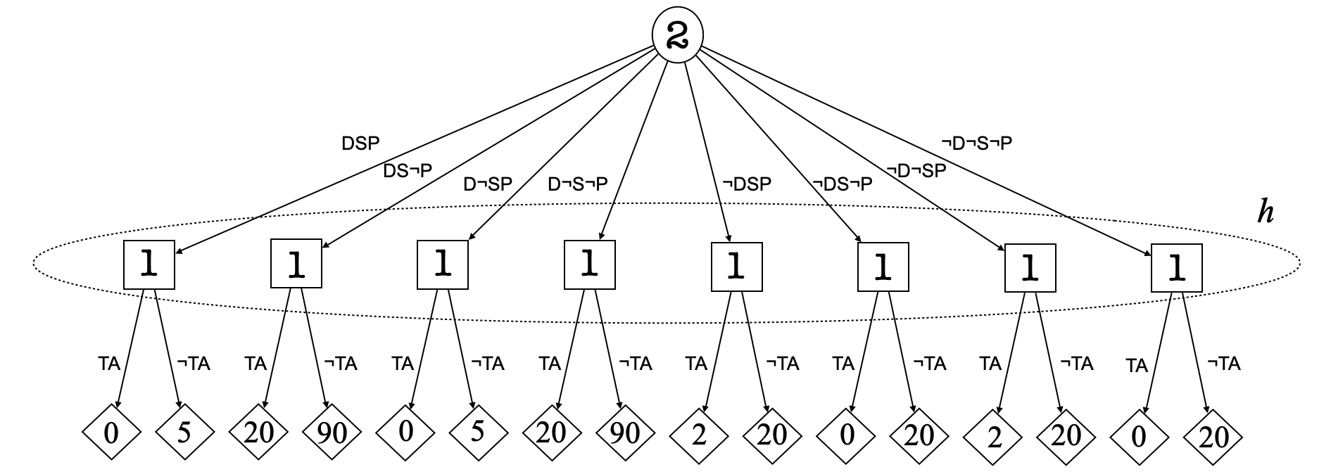
Figure 4: The game tree obtained from Figure 1.

Observe that every non-terminal node is labeled by the player which controls it in the influence diagram. Moreover, shapes of the node for players correspond to the shape of the nodes (i.e., 1 and 2) that they control in the ID. In parallel, leaf nodes $\ell\in\mathcal{L}$ which represent outcomes are diamond-shaped. Since the root node in the ID (in Figure 1), player 2 (nature) is the root node in the game tree.

We introduce some necessary notions for computing the cost minimization problem with arbitrary strategies. A move $\mathsf{\omega}$ is an edge in the game tree, and corresponds to a value of a particular decision node in an ID i.e., $\mathsf{\omega}\in val(d)$. A sequence $\sigma$ is a path (a sequence of moves) in the game tree. For example, the empty sequence $\emptyset$ and $\textsf{DS}\neg\textsf{PTA}$ are sequences in Figure 4. A sequence of player $i$ is the sequence $\sigma_{i}$ of its moves along the game tree e.g., $\textsf{DS}\neg\textsf{P}$ for $\sigma_{2}$ and TA for $\sigma_{1}$. We denote all possible sequences of Player 1 and Player 2, by $\mathcal{S}_{1}$ and $\mathcal{S}_{2}$, respectively. Given a leaf node $\ell\in\mathcal{L}$, we denote the sequence which reaches $\ell$ by $\sigma(\ell)$, and $\sigma_{i}(\ell)$ denotes the sequential moves of Player $i$. We refer to the content of such a leaf, as $c(\ell)\in val(c)$, after the cost function $c$.

An information set is a set of nodes in which a player has the same moves e.g., oval $h$ in Figure 4. In our case, we collapse information sets to singletons since Player 1 (the agent in ID) has access to the conditional probability distribution of each chance node. In game-theoretic terms, this correspond to perfect information game where Player 1 can observe what Player 2 has chosen. We denote available moves for a player $i$ in an information set $h$ as $\mathsf{\Omega}_{h}$ which corresponds to values of a particular node $d$ in the ID, and the set of its information sets as $H_{i}$. If both players can remember all of their moves along the path of the game tree, the game has perfect recall. Intuitively, it means that no player can get additional information about their position in the game three by remembering earlier actions. Observe that this is indeed inline with our initial assumption of no forgetting.

We translate the conditional distributions in the ID to the game tree in a way that it simulates the overall behaviour faithfully. We use the well-known notion of behaviour strategy in extended-form games. A behaviour strategy is a probability distribution $\beta$ on the next available moves in a state in the game tree. For instance, in Figure 4, the probability that the move $\textsf{DS}\neg\textsf{P}$ is taken can be chosen w.r.t. the ID in Figure 1 and the strategy $S$, which would be, then, 0.012. Hence $\beta_{2}(\textsf{DS}\neg\textsf{P})=0.012$ where $\beta_{2}$ is the behavior strategy for Player 2. Obviously, a behaviour strategy $\beta_{i}$ for player $i$ satisfies the following: $\sum_{\mathsf{\omega}\in\mathsf{\Omega}_{h}}\beta_{i}(\mathsf{\omega})=1$ and $\beta_{i}(\mathsf{\omega})\geq 0$ for all $h\in H_{i}$, $\mathsf{\omega}\in\mathsf{\Omega}_{h}$. Then by extending behaviour strategies to sequences, we obtain realization probability of a sequence $\sigma$ of Player $i$ under $\beta_{i}$: $\beta_{i}(\sigma):=\Pi_{\mathsf{\omega}\in\sigma}\beta_{i}(\mathsf{\omega})$ which is in line with the standard chain rule. Note that $\beta_{i}(\emptyset)=1$ for any $\beta_{i}$. In terms of the game tree, the expected cost (in Definition 2) can be rewritten as

$$\sum_{\ell\in\mathcal{L}}c(\ell)\cdot\beta_{1}(\ell)\cdot\beta_{2}(\ell).$$ (1)

Moreover, given a $h\in H$ and a sequence $\sigma\mathsf{\omega}$ being an extension of sequence $\sigma\in h$ with a move $\mathsf{\omega}$, then we define

$$\beta_{i}(\sigma):=\Sigma_{\mathsf{\omega}\in h}\beta_{i}(\sigma\mathsf{\omega}).$$ (2)

We define $\beta_{i}(\sigma^{\prime})=0$ for any non-realizable sequence $\sigma^{\prime}$. Then any $\mu_{1}$ being a vector value of such a $\beta_{1}$ (hence for Player 1) is called a realization plan. This is analogous for Player 2, but since it is indifferent for any outcome, and observing that its realization plan is fixed, considering only the expected cost minimization of Player 1 fulfills our goals. We can represent the cost of player 1 in terms of a cost matrix $C$, as follows. For every leaf node $\ell\in\mathcal{L}$ in $\mathcal{G}_{\mathcal{D}}$, the entries $c_{\sigma_{1}(\ell)\sigma_{2}(\ell)}:=c(\ell)$ construct a $|\mathcal{S}_{1}|\times|\mathcal{S}_{2}|$ matrix. The expected cost of Player 1 is $\mu_{1}^{\top}(C\mu_{2})$ where $\mu_{1}$ is the realization plan of Player 1 (a global strategy), $C$ is the cost matrix, and $\mu_{2}$ is the realization plan of nature (chance nodes).

We now have all we need to formulate the expected cost minimization problem of Player 1 in terms of linear constraints. Given a fixed realization plan $\mu_{2}$,

$$\min\mu_{1}(C\mu_{2})\text{ subject to }R\cdot\mu_{1}=r,\text{ }\mu_{1}\geq 0$$ (3)

where $R$ is the matrix for realization constraints i.e., columns correspond to elements of $S_{1}$, and rows are of size $|H_{1}|+1$. Intuitively, the first row of $R$ and $r$ implements $\beta_{i}(\emptyset)=1$, and the remaining rows implement Equation 2 in the form of for $-\beta_{1}(\sigma)+\sum_{\mathsf{\omega}\in\mathsf{\Omega}_{h}}\beta_{1}(\sigma\mathsf{\omega})$ = 0 for every $h\in H_{1}$ and 0 is the zero vector. And optimal mixed-strategy is a strategy that is a solution for the LP given in Equation 3. Realize that the size of LP is linear in the size of the game tree. However, game tree grows exponentially for a given ID, realising every valuation of its conditional dependency tables. Hence, hardness remains. In parallel, recall that mixed-strategies also include pure strategies. Hence, PSpace-completeness remains. Yet one can easily modify the LP given above to fully-mixed strategies by setting $\mu_{1}>0$ i.e., requiring every component of the strategy to be greater than zero. To apply these results to $\text{ID-}\mathcal{E\!L}$, we simply modify the linear program to consider the evidence of the context that is given by the observations of the results. Hence, all problems are still solvable in polynomial space.

5 Related Work

In addition to the probabilistic logics mentioned in the introduction, some earlier works (?; ?) employed (probabilistic) DLs in a decision-theoretic setting. However, neither addressed observations, nor contextual reasoning. Hence, they stay completely orthogonal to our work.

Earlier work (?; ?) has used IDs in a game-theoretic setting, yet in a different direction: to represent sequential games with more than $n\geq 2$ players compactly and to solve them. We borrow (in Section 4) the notion of game-tree from game theory to compute arbitrary strategies in IDs. There we simulate the ID as a 2-player game (against nature) in a game-tree, which allows us to employ linear programming based solution. These works also do not consider contextual reasoning (since this is not their motivation). To our knowledge, the closest work is (?) which is of no surprise, since we propose its decision-theoretic extension.

6 Conclusions

We introduced $\text{ID-}\mathcal{E\!L}$, a new extension of the light-weight DL $\mathcal{E\!L}$ capable of modeling and dealing with decision situations under uncertainty. This is achieved by integrating an influence diagram to represent the uncertainty, potential decisions, and the overall costs of a choice into the knowledge base. The ontological ($\mathcal{E\!L}$) portion and the influence representation are combined through the use of contexts, which express the situations in which knowledge is required to hold. From an abstract point of view, we build a collection of ontologies, which are necessarily true only in specific contexts; but, in line with the open-world assumption, could still be verified in other situations. These ontologies contain only certain knowledge (i.e., there is no mention of uncertainty within the ontological knowledge), but the specific context under consideration is uncertain.

Extending the basic idea of the probabilistic DL $\mathcal{BE\!L}$, our framework allows for an agent to influence its context through choices in specific nodes of the network, trying to minimise the overall expected cost over the network. Intuitively, this means minimising the probability of large costs, and maximising the probability of low costs. Obviously, the framework remains uncertain, and there is no absolute guarantee that the observation of the environment do yield the lowest possible cost. But the agent can only influence its own choices, not those of the environment.

For this paper, we studied the basic reasoning problems in this logic, and gave tight complexity bounds for all of them. Interestingly, the decision problem associated with finding a dominating optimal strategy, in which the agent should find the best strategy conditioned on an ontological observation, remains PSpace-complete, just as in making inferences over an ID. A practical algorithm for solving this problem—and its effective implementation—is left for future work. As future work we will also consider other decision-based reasoning tasks, and complexity classes. Notably, we will study whether optimal strategies or costs can be approximated efficiently, and whether reasoning becomes tractable over some given parameters. We note that this is still an open problem even for the special case of $\mathcal{BE\!L}$. For example, inferences on a Bayesian network are tractable over a bounded tree-width, but this property is lost in the currently known algorithms for reasoning in $\mathcal{BE\!L}$ (?).

Another task to consider is that of building strategies iteratively, as a response to the environment; this is justified by the no-forgetting assumption of IDs, and allows an agent to react to newer observations, rather than designing an overall strategy from the beginning. Some of the complexity issues highlighted in this paper can be alleviated in this way. Another interesting issue to resolve is how to dislodge the strategies from the underlying ID, and allow the agent to select consequences (rather than direct contexts) instead.

To conclude, we note that the choice of $\mathcal{E\!L}$ as a logical formalism is motivated by its polynomial-time reasoning problems, which allow us to understand complexity issues better. Likewise, considering TBoxes exclusively, without the addition of ABoxes was a design choice to simplify the introduction of the formalism. However, our framework can be combined with other (potentially more expressive) logics, akin to what was done for Bayesian DLs (?; ?). Building those extensions introduces further problems (e.g., consistency) that would need to be studied in detail as well.

References

- Acar et al. 2017 Acar, E.; Fink, M.; Meilicke, C.; Thorne, C.; and Stuckenschmidt, H. 2017. Multi-attribute decision making with weighted description logics. IfCoLog Journal of Logics and its Applications 4(7):1973–1996.
- Acar, Thorne, and Stuckenschmidt 2015 Acar, E.; Thorne, C.; and Stuckenschmidt, H. 2015. Towards decision making via expressive probabilistic ontologies. In International Conference on Algorithmic Decision Theory, 52–68. Springer.
- Baader et al. 2007 Baader, F.; Calvanese, D.; McGuinness, D.; Nardi, D.; and Patel-Schneider, P., eds. 2007. The Description Logic Handbook: Theory, Implementation, and Applications. Cambridge University Press, second edition.
- Baader, Brandt, and Lutz 2005 Baader, F.; Brandt, S.; and Lutz, C. 2005. Pushing the envelope. In Kaelbling, L., and Saffiotti, A., eds., Proc. 19th Int. Joint Conf. on Artificial Intelligence (IJCAI’05), 364–369. Professional Book Center.
- Baader, Knechtel, and Peñaloza 2012 Baader, F.; Knechtel, M.; and Peñaloza, R. 2012. Context-dependent views to axioms and consequences of semantic web ontologies. Journal of Web Semantics 12:22–40.
- Botha, Meyer, and Peñaloza 2019 Botha, L.; Meyer, T.; and Peñaloza, R. 2019. A Bayesian extension of the description logic ALC. In Proceedings of the 16th European Conference on Logics in Artificial Intelligence (JELIA’19), volume 11468 of Lecture Notes in Computer Science, 339–354. Springer.
- Ceylan and Peñaloza 2014a Ceylan, İ. İ., and Peñaloza, R. 2014a. The Bayesian description logic BEL. In Demri, S.; Kapur, D.; and Weidenbach, C., eds., Proceedings of the 7th International Joint Conference on Automated Reasoning (IJCAR’14), volume 8562 of Lecture Notes in Computer Science, 480–494. Springer.
- Ceylan and Peñaloza 2014b Ceylan, İ. İ., and Peñaloza, R. 2014b. Bayesian description logics. In Proceedings of the 27th International Workshop on Description Logics (DL’ 14), volume 1193 of CEUR Workshop Proceedings, 447–458. CEUR-WS.org.
- Ceylan and Peñaloza 2014c Ceylan, İ. İ., and Peñaloza, R. 2014c. Reasoning in the description logic BEL using Bayesian networks. In Proceedings of the 2014 AAAI Workshop on Statistical Relational Artificial Intelligence, volume WS-14-13 of AAAI Workshops. AAAI.
- Ceylan and Peñaloza 2017 Ceylan, İ. İ., and Peñaloza, R. 2017. The Bayesian ontology language BEL. Journal of Automated Reasoning 58(1):67–95.
- d’Amato, Fanizzi, and Lukasiewicz 2008 d’Amato, C.; Fanizzi, N.; and Lukasiewicz, T. 2008. Tractable reasoning with bayesian description logics. In Greco, S., and Lukasiewicz, T., eds., Proceedings of the Second International Conference on Scalable Uncertainty Management (SUM 2008), volume 5291 of Lecture Notes in Computer Science, 146–159. Springer.
- Fudenberg and Tirole 1991 Fudenberg, D., and Tirole, J. 1991. Game Theory. MIT Press.
- Gutiérrez-Basulto et al. 2017 Gutiérrez-Basulto, V.; Jung, J. C.; Lutz, C.; and Schröder, L. 2017. Probabilistic description logics for subjective uncertainty. Journal of Artificial Intelligence Research 58:1–66.
- Koller and Milch 2003 Koller, D., and Milch, B. 2003. Multi-agent influence diagrams for representing and solving games. Games and economic behavior 45(1):181–221.
- Littman, Majercik, and Pitassi 2001 Littman, M. L.; Majercik, S. M.; and Pitassi, T. 2001. Stochastic Boolean satisfiability. Journal of Automated Reasoning 27(3):251–296.
- Lukasiewicz and Straccia 2008 Lukasiewicz, T., and Straccia, U. 2008. Managing uncertainty and vagueness in description logics for the semantic web. Journal of Web Semantics 6(4):291–308.
- Maschler, Solan, and Zamir 2013 Maschler, M.; Solan, E.; and Zamir, S. 2013. Game theory (translated from the hebrew by ziv hellman and edited by mike borns). Cambridge University Press, Cambridge, pp. xxvi 979:4.
- Niepert, Noessner, and Stuckenschmidt 2011 Niepert, M.; Noessner, J.; and Stuckenschmidt, H. 2011. Log-linear description logics. In Twenty-Second International Joint Conference on Artificial Intelligence.
- Nisan et al. 2007 Nisan, N.; Roughgarden, T.; Tardos, E.; and Vazirani, V. V. 2007. Algorithmic Game Theory. New York, NY, USA: Cambridge University Press.
- Pearl 1988 Pearl, J. 1988. Probabilistic Reasoning in Intelligent Systems: Networks of Plausible Inference. San Francisco, CA, USA: Morgan Kaufmann Publishers Inc.
- Riguzzi et al. 2015 Riguzzi, F.; Bellodi, E.; Lamma, E.; and Zese, R. 2015. Probabilistic description logics under the distribution semantics. Semantic Web 6(5):477–501.
- Savitch 1970 Savitch, W. J. 1970. Relationships between nondeterministic and deterministic tape complexities. Journal of Computer and System Sciences 4(2):177 – 192.
- Shachter 1986 Shachter, R. D. 1986. Evaluating influence diagrams. Operations Research 34(6):871–882.
- Shannon 1949 Shannon, C. E. 1949. The synthesis of two-terminal switching circuits. Bell System Technical Journal 28(1):59–98.
- Zhou, Lü, and Liu 2013 Zhou, L.; Lü, K.; and Liu, W. 2013. Game theory-based influence diagrams. Expert Systems 30(4):341–351.