Infrared Telescope Facility (IRTF) spectral library II:

Abstract

Context. Stellar population studies in the infrared (IR) wavelength range have two main advantages with respect to the optical regime: they probe different populations, because most of the light in the IR comes from redder and generally older stars, and they allow us to see through dust because IR light is less affected by extinction. Unfortunately, IR modeling work was halted by the lack of adequate stellar libraries, but this has changed in the recent years.

Aims. Our project investigates the sensitivity of various spectral features in the 1–5 $\mu$m wavelength range to the physical properties of stars ($T_{\rm eff}\,$, [Fe/H], $\log{g}\,$) and aims to objectively define spectral indices that can characterize the age and metallicity of unresolved stellar populations.

Methods. We implemented a method that uses derivatives of the indices as functions of $T_{\rm eff}\,$, [Fe/H] or $\log{g}\,$across the entire available wavelength range to reveal the most sensitive indices to these parameters and the ranges in which these indices work.

Results. Here, we complement the previous work in the I and K bands, reporting a new system of 14, 12, 22, and 12 indices for Y, J, H, and L atmospheric windows, respectively, and describe their behavior. We list the equivalent widths of these indices for the Infrared Telescope Facility (IRTF) spectral library stars.

Conclusions. Our analysis indicates that features sensitive to the effective temperature are present and measurable in all the investigated atmospheric windows at the spectral resolution and in the metallicity range of the IRTF library for a signal-to-noise ratio greater than 20-30. The surface gravity is more challenging and only indices in the H and J windows are best suited for this. The metallicity range of the stars with available spectra is too narrow to search for suitable diagnostics. For the spectra of unresolved galaxies, the defined indices are valuable tools in tracing the properties of the stars in the IR-dominant stellar populations.

1 Introduction

The extension of stellar evolutionary models towards the observationally challenging infrared (IR) regime is driven by the fact that optical and IR light originate from different types of stars, allowing us to obtain independent constraints on young and old stellar populations. Another reason to venture into the IR region is to penetrate the dust in galaxies with heavy extinction (e.g., Engelbracht et al., 1998; Ivanov et al., 2000). Furthermore, new sets of galaxy spectra with better quality than before become available in the IR, posing further challenges to modeling (e.g., François et al., 2019).

The interpretation of these data requires both understanding of the complex physical processes in galaxies and a significant observational effort to build libraries of IR stellar spectra. In recent times, technological improvements have allowed significant advances in both these areas. The Infrared Telescope Facility (IRTF) stellar library (Cushing et al., 2005; Rayner et al., 2009) offered 226 stellar and brown dwarf spectra with a resolving power of $R\sim 2000$ over $\lambda$=1-5 $\mu$m. Conroy & van Dokkum (2012), Röck et al. (2015, 2016), and Vazdekis et al. (2016) incorporated the IRTF library into their models. To improve the short metallicity range of the IRTF library, Villaume et al. (2017) presented a new IRTF library with an extended metallicity range ($-1.7\leq[Fe/H]\leq 0.6$ dex). This library allows us to expand the stellar population models to wide metallicity and wavelength ranges (Conroy et al., 2018).

The X-SHOOTER Spectral Library (XSL, Chen et al., 2011; Arentsen et al., 2019) and its later releases (Chen et al., 2014; Gonneau et al., 2020) also extends into the IR ($\lambda$=0.3-2.5 $\mu$m), although with a somewhat higher resolving power of $R\sim 10,000$. In Cesetti et al. (2013, hereafter Paper I), we investigated the sensitivity of the features in the I and K atmospheric windows to the stellar physical parameters using the method of “sensitivity functions” – derivatives of the changes in the spectra with respect to the effective temperature $T_{\rm eff}\,$, surface gravity $\log{g}\,$, and to some extent (because of the limited metallicity spread in the IRTF library) to the metallicity [Fe/H]. Indeed, the hydrogen, Na, Ca, and CO features turned out to be the best $T_{\rm eff}\,$indicators, and we highlighted that some Mg and Fe features can serve the same purpose. We confirmed that the well-known Ca lines and CO bands were the best $\log{g}\,$indicators and we demonstrated the surface gravity sensitivity of the FeClTi feature at 0.908–0.910 $\mu$m. The most promising abundance indicators were of course the Ca, Fe, and Mg lines, but the limited [Fe/H] range (from $-$0.6 to 0.4 dex) prevented us from deriving firm conclusions.

In this paper, we complete the exploration of the IRTF libraries, defining indices optimized for stellar population analysis in the Y, J, H, and L atmospheric windows. Our work constitutes a preparation for the wealth of data expected from the new generation of instruments like the Multi-Object Optical and Near-IR Spectrograph (MOONS; Cirasuolo et al., 2011) at the Very Large Telescope, the Infrared Multi-Object Spectrograph (IRMS; Mobasher et al., 2010) at the Thirty Meter Telescope, and the ELT Adaptive optics for GaLaxy Evolution (EAGLE; Cuby et al., 2010) at the Extreme Large Telescope (ELT) that will make it possible to measure spectral features of $\alpha$- and iron-group elements of a large number of galaxies, and even of individual red super giants to tens of megaparsecs (Evans et al., 2011). Here, we provide the basis for these near-future facilities. Furthermore, we also investigate the mid-IR L window features that will be accessible with the James Webb Space Telescope.

Section 2 briefly describes the properties of the IRTF spectral library. The main spectral features of the Y, J, K, and L atmospheric windows, sensitivity map analysis, and their use as spectral diagnostics are discussed in Sects. 3, 4, and 7, respectively. Index definition and measurements and their sensitivity to the galaxy broadening velocity are described in Sects. 5 and 6 respectively. Section 8 describes and discusses our results. Due to the large number of results we included in the text only those for the Y band, and we moved all the figures for the J, H, and L bands to Sect. Infrared Telescope Facility (IRTF) spectral library II:. The plots of the model spectra and of the sensitivity maps are shown in Appendices A and B respectively. The plots of the broadening effects are shown in Appendix C and the behavior of the spectral indices in Appendix D. Finally the values of the measured indices in the different bands are reported in Appendix E.

2 IRTF spectral library and analysis method

The IRTF spectral library (Cushing et al., 2005; Rayner et al., 2009) contains flux calibrated spectra of about 200 objects, with a typical uncertainty of about 5 %. The analysis of the spectra and methodology adopted in this work are the same as in Paper I. In this section, we give a short summary, while we refer to Paper I for a detailed description of the performed steps.

The spectra were re-binned and normalized to unity at regions free of absorption features, in order to reduces the scatter in our final analysis. We then assembled the available spectral types (Spt), $T_{\rm eff}\,$, $\log{g}\,$, [Fe/H], $M_{V}$ , and parallaxes for the sample stars from the literature (Paper I, Table 3), typically derived from high-resolution optical spectroscopy.

Following the convention adopted in Paper I, we quantified the spectral types with two parametrizations. One is based on the corresponding effective temperature and the other on a quantitative analog SpT of the spectral classes, as follows: SpT=0 for F0 stars, 1 for G0, 2 for K0, and so on, with decimals for the sub-types (e.g., SpT=0.5 for F5; 1.8 for G8; 3.05 for M0.5).

Our method is a generalization of the sensitivity indices applied first by Worthey et al. (1994a, see their Tables 2 and 3), which are simple derivatives of the index strength with respect to the physical parameter of interest (e.g., $T_{\rm eff}\,$, [Fe/H], $\log{g}\,$): a positive/negative sensitivity index implies that the feature becomes stronger/weaker with an increasing parameter value, while zero means no dependence.

We improved this method, applying it directly to the spectra in the wavelength space. To provide continuity across the entire parametric space we first generated semi-continuous sets of interpolated spectra (called model spectra in Paper I), which were constructed by least-square fitting of the normalized intensity with a second-order polynomial as a function of spectral type (SpT), surface gravity, or temperature for each wavelength bin independently, and then combining in the wavelength space the polynomial fits for all wavelength bins. Finally, the sensitivity map was obtained by calculating the derivatives of the interpolated spectra with respect to spectral type, surface gravity, or temperature.

Following the sensitivity map, we identify spectral regions sensitive to a given physical parameter (they appear as sharp features on the respective sensitivity map) and we defined the indices accordingly to encompass these regions. Adopting the same approach as Paper I, we decided to define narrow width indices instead of intermediate width indices. Broader indices do boost the signal-to-noise ratio (S/N), but they were mostly investigated with lower resolution spectrographs (e.g., Wing & Spinrad, 1970; Lançon et al., 2007) of the past generation, so we decided to concentrate on the narrow width indices taking advantage of the higher resolution of our spectra.

It should be noticed that in Paper I we were forced to limit the analysis of the metallicity effects, because of the narrow [Fe/H] range spanned by the IRTF stars. We decided to adopt the same library in this second paper to perform an homogeneous analysis in all the atmospheric windows. In a forthcoming paper, we will extend the investigation of the metallicity effects to the wider [Fe/H] range spanned by the new extended IRTF stellar library (Villaume et al., 2017).

3 Main spectral features in Y, J, H, and L atmospheric windows

In this section we give a brief review of the charachteristics of the atmospheric windows considered in the paper and we describe their main spectral features.

3.1 Y atmospheric window

The spectral region around 1 $\mu$m has long been neglected, because it falls in between the optical and IR regimens where for a long time detector technology did not work well. The photometric $Y$ filter centered at 1.035 $\mu$m (with a full whidth half maximum (FWHM) of $\sim 0.13\,\mu$m) was introduced by Hillenbrand et al. (2002) to take advantage of the better atmospheric transmission in that region. They also investigated which features dominate the spectra of cool stars and brown dwarfs at $\lambda$$\sim$0.97-1.07 $\mu$m. A few low- and medium-resolution spectral libraries of late-type stars covered this spectral region (Leggett et al., 1996; Joyce et al., 1998; Lançon & Wood, 2000; McLean et al., 2003; Cushing et al., 2005; Lodieu et al., 2005). More recently, Sharon et al. (2010) published a high-resolution (R$\sim$25,000) atlas for the full range of luminosity classes of F, G, K, and M stars. The XSL also covers the Y window (Chen et al., 2014; Arentsen et al., 2019). We note that here and in the following we only mention works that include a few tens or more stars and that span many SpT and/or luminosity classes, because only these libraries are actually of interest for stellar population studies.

The strongest absorption features in the Y atmospheric window ($\sim$0.94–1.10 $\mu$m) are the H lines Pa$\gamma$, Pa$\delta$, and Pa$\epsilon$. There are also many low and moderate excitation lines of neutral metals, such as Cai, Cri, Fei, Ki, Mgi, Nai, Nii, Sii, and Tii along with singly ionized Srii (Leggett et al., 1996; Lyubchik et al., 2004). The spectra show molecular bands, including the first-overtone band heads of CN extending redward at 1.097$\,\mu$m (McKellar, 1988). For the later SpTs, the Y window contains TiO bands that appear at 0.982$\,\mu$m and 1.014$\,\mu$m, FeH band-head appearing at 0.989$\,\mu$m (Leggett et al., 1996), and VO bands at 1.06$\,\mu$m (Leggett et al., 1996; Cushing et al., 2005; Rayner et al., 2009). Finally, broad H₂O absorption bands appear on both sides of the Y window. Generally, the H lines are stronger in F- and G-type stars, while the metal and molecular features are more relevant in K- and M-type stars.

The Y atmospheric window interpolated spectra for the different SpTs (i.e., for different $T_{\rm eff}$) for supergiant, giant, and dwarf stars are shown in Figs. 1, 10, and 11, respectively.

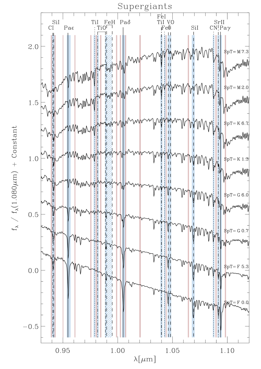
Figure 1: Y atmospheric window model spectra of supergiants obtained by fitting at each wavelength the flux-normalized (at 1.08$\,\mu$m) sample spectra along SpTs. The model spectra for different SpTs are offset for displaying purposes and the SpTs are given on the right. The green regions mark the bandpasses of the newly defined indices, the gray regions mark their adjacent continuum as defined in this paper (see Table 1). Some relevant absorption features are marked. Here and for the other bands we did not consider features at the edges of the windows, because they can be affected by variable atmospheric transmission. The plots for stars of other luminosity classes and atmospheric windows are shown in Appendix A.

Table 1: Definition of the spectral indices. We have marked with the symbol ^‡ the index definitions similar to Riffel et al. (2019), with the symbol ^△ those similar to Origlia et al. (1993b), with the symbol ^□ those similar to Ivanov et al. (2004), with the symbol ^† those similar to Conroy & van Dokkum (2012) and Villaume et al. (2017), and with the symbol ^♢ those similar to McLean et al. (2003) and Cushing et al. (2005).

Index	Species	Bandpass   Definitions   ($\mu$m)		Index	Species	Bandpass   Definitions   ($\mu$m)
Name		Central	Blue and Red Continua	Name		Central	Blue and Red Continua
Y atmospheric window				H atmospheric window (cont):
CSi	Ci+Sii	0.9400-0.9424	0.9390-0.9399  0.9425-0.9434	Br16	Hi(n=4)	1.552-1.557	1.548-1.550  1.593-1.594
Pa$\epsilon$	Hi(n=3)	0.9535-0.9570	0.9498-0.9504  0.9606-0.9614	CO1‡	12CO(2,0)	1.557-1.5635	1.548-1.550  1.593-1.594
Ti	Tii	0.9780-0.9795	0.9750-0.9760  0.9800-0.9810	Br15	Hi	1.567-1.572	1.548-1.550  1.593-1.594
TiO A	TiO	0.9812-0.9826	0.9800-0.9810  0.9840-0.9850	Mg3‡	Mgi	1.573-1.580	1.548-1.550  1.593-1.594
TiO B	TiO	0.9885-0.9900	0.9840-0.9850  0.9985-0.9995	FeH1‡△□	FeH	1.582-1.586	1.548-1.550  1.593-1.594
FeH†♢	FeH	0.9900-0.9950	0.9840-0.9850  0.9985-0.9995	Si‡△□	Sii	1.587-1.591	1.548-1.550  1.593-1.594
Pa$\delta$	Hi(n=3)	1.0040-1.0067	1.0020-1.0030  1.0067-1.0077	CO2‡	12CO(2,0)	1.595-1.600	1.593-1.594  1.616-1.618
FeTi	Fei+Tii	1.0390-1.0408	1.0198-1.0210  1.0438-1.0446	Fe2	Fei	1.605-1.609	1.593-1.594  1.616-1.618
Fe	Fei	1.0422-1.0436	1.0198-1.0210  1.0438-1.0446	Br13	Hi(n=4)	1.610-1.614	1.593-1.594  1.616-1.618
VO	VO	1.0456-1.0488	1.0438-1.0446  1.0640-1.0650	CO3△	12CO(2,0)	1.618-1.622	1.616-1.618  1.634-1.637
Si‡	Sii	1.0676-1.0702	1.0640-1.0650  1.0892-1.0902	FeH2	FeH	1.624-1.628	1.616-1.618  1.634-1.637
CN	CN	1.0868-1.0882	1.0640-1.0650  1.0892-1.0902	CO4	12CO(2,0)	1.639-1.647	1.634-1.637  1.6585-1.6605
Sr	Srii	1.0913-1.0923	1.0892-1.0902  1.0978-1.0988	Fe3	Fei	1.651-1.658	1.634-1.637  1.6585-1.6605
Pa$\gamma$	Hi(n=3)	1.0930-1.0950	1.0892-1.0902  1.0978-1.0988	CO5	12CO(2,0)	1.6605-1.6640	1.6585-1.6605  1.6775-1.679
				Al1	Ali	1.6705-1.6775	1.6585-1.6605  1.6775-1.679
J atmospheric window				Br11	Hi(n=4)	1.6790-1.6825	1.6775-1.679  1.6825-1.6835
Na‡†	Nai	1.1358-1.1428	1.1320-1.1340  1.1430-1.1460	COMg□	12CO(2,0)	1.705-1.713	1.692-1.696  1.714-1.716
FeCr‡	Fei+Cri	1.1600-1.1624	1.1560-1.1585  1.1716-1.1746		+Mgi
K1 A†♢	Ki	1.1670-1.1714	1.1560-1.1585  1.1716-1.1746	Br10	Hi(n=4)	1.735-1.739	1.725–1.728  1.744–1.748
C	Ci	1.1746-1.1765	1,1716-1.1746  1.1805-1.1815
K1 B†♢	Ki	1.1765-1.1800	1.1716-1.1746  1.1805-1.1815	L atmospheric window
Mg‡	Mgi	1.1820-1.1840	1.1805-1.1815  1.1855-1.1875	Mg1‡	Mgi	3.388-3.406	3.360-3.376  3.425-3.440
Si‡	Sii	1.1977-1.2004	1.1910-1.1935  1.2050-1.2070	Mg2‡	Mgi	3.454-3.464	3.425-3.440  3.476-3.496
SiMg	Sii+Mgi	1.2070-1.2095	1.2050-1.2070  1.2150-1.2180	P16	OH(1-0) P16	3.514-3.532	3.476-3.496  3.540-3.560
K2 A‡♢	Ki	1.2415-1.2455	1.2350-1.2380  1.2460-1.2490	P14	OH(2-1) P14	3.564-3.582	3.540-3.560  3.604-3.612
K2 B♢	Ki	1.2495-1.2540	1.2460-1.2490  1.2560-1.2580	P17	OH(1-0) P17	3.582-3.597	3.540-3.560  3.604-3.612
Pa$\beta$‡	Hi(n=3)	1.2795-1.2840	1.2755-1.2780  1.2855-1.2873	P15	OH(2-1) P15	3.628-3.648	3.604-3.612  3.665-3.673
Al‡†	Ali	1.3115-1.3168	1.3050-1.3075  1.3230-1.3250	Pf$\gamma$	Hi(n=5)	3.736-3.745	3.718-3.728  3.793-3.803
				Mg3‡	Mgi	3.862-3.870	3.840-3.850  3.870-3.880
H atmospheric window				Hu15	Hi(n=6)	3.900-3.914	3.870-3.880  3.914-3.922
Mg1‡	Mgi	1.485-1.491	1.483-1.485  1.491-1.500	SiO1	SiO(2,0)	3.998-4.012	3.990-3.998  4.025-4.035
Mg2‡□	Mgi	1.500-1.508	1.491-1.508  1.510-1.512	SiO2	SiO(3,1)	4.035-4.050	4.025-4.035  4.060-4.070
K1	Ki	1.515-1.520	1.510-1.512  1.523-1.525	SiO3	SiO(4,2)	4.080-4.090	4.060-4.070  4.095-4.105
Fe1	Fei	1.528-1.533	1.523-1.525  1.548-1.550

3.2 J atmospheric window

Photometrically, the first practical exploration of the J window ($\lambda\sim 1.11-1.33\,\mu$m) dates back to Fellgett (1951). Johnson (1966) defined the precursors of the $JHK$ filters used today. The J window is relatively free of telluric features compared with the other parts of the IR, and this makes it more valuable for quantitative spectroscopy. The first spectroscopic atlas of stars observed in the IR was published by Johnson & Méndez (1970). A number of other spectral libraries covered it before the IRTF library (Leggett et al., 1996; Joyce et al., 1998; Lançon & Wood, 2000; McLean et al., 2003; Lodieu et al., 2005; Lançon et al., 2007; Ranade et al., 2007; Lebzelter et al., 2012). The work of Wallace et al. (2000) stands out because their spectra have higher resolving power ($R\sim 3000$) and better S/N. The XSL also covers the J window (Chen et al., 2014).

A prominent feature of F and G stars in the J window is the Pa$\beta$ at 1.282 $\mu$m, whose strength decrease toward late sub-types. It becomes very weak in K stars and is absent for M stars whose spectra are dominated by lines of neutral metal species of lower ionization potential. Notable atomic features in the spectra of K and M stars are the Nai doublet at 1.14 $\mu$m, the Ki doublet at 1.18 $\mu$m and 1.25 $\mu$m, and the Ali doublet at 1.313 $\mu$m and 1.318 $\mu$m. They are strongest in late-M dwarfs and weaker in corresponding giants and supergiants. Therefore, they are excellent luminosity class (or surface gravity) indicators. The Sii features appear in early F stars and fade in early M stars. We also see some Fei, Mgi, Tii, and Mni lines, but they are too weak to be suitable for extragalactic work.

At the resolution of our data, a number of spectral features are blends of absorption lines from different chemical elements. For example, the feature at $\sim$1.169 $\mu$m is due primarily to Ci in F and G stars. However, for later spectral types, Ki absorption plays the dominant role in determining the feature strength. The Al, Mn, Fe, and Mg lines behave similarly to Si, but persist through the latest observed types. The continuum shape in the J window is redder toward later spectral type. The J atmospheric window interpolated spectra for the different SpTs (i.e., for different $T_{\rm eff}$) for supergiant, giant, and dwarf stars are shown in Figs. 12, 13, and 14, respectively.

3.3 H atmospheric window

The photometric use of the H window ($\lambda\sim$1.48-1.78 $\mu$m) also goes back to Fellgett (1951) and Johnson (1966), but the spectroscopic treatment is more difficult than the J window because it contains more telluric absorptions. Furthermore, the background emission is due to numerous O₂H and OH lines that vary on a timescale of a few minutes, making the data processing more challenging.

Although the K window ($\lambda\sim 1.92-2.40\,\mu$m) is the most studied, the presence of circumstellar dust or active galactic nuclei (AGN) often results in a significant excess of continuum emission at $\lambda$$\geq$2 $\mu$m (Schinnerer et al., 1997; Ivanov et al., 2000). This excess weakens or even renders invisible the photospheric absorption features, making the K window unsuitable for stellar population studies. Yet, the radiation from the stellar photospheres still dominates shorter wavelengths in the H window. This motivated the first studies of star spectra in the H window (e.g., Johnson & Méndez, 1970; Lancon & Rocca-Volmerange, 1992; Origlia et al., 1993a; Dallier et al., 1996; Morris et al., 1996; Blum et al., 1997; Meyer et al., 1998; Blum et al., 1997; Meyer et al., 1998). More recently, a number of spectral libraries have been reported for wide varieties of stars (e.g., Ivanov et al., 2004; Ranade et al., 2004; Lodieu et al., 2005; Hanson et al., 2005; Venkata Raman & Anandarao, 2008; Huynh et al., 2011; Cooper et al., 2013; Ghosh et al., 2019). The spectral libraries of Lebzelter et al. (2012) and Park et al. (2018) stand out because of their significantly higher resolving power of $R\sim 100,000$ and $45,000$, respectively. However, they contain less stars and are not really suitable for galaxy population modeling.

A large effort was devoted to abundance studies of red giants and supergiants because of the rich concentration of both molecular and metal lines in the H window (Origlia et al., 1993a, 2002, 2003; Origlia & Rich, 2004; Cunha et al., 2007; Davies et al., 2009a, b). High-resolution spectra in the H-band domain enabled the Apache Point Observatory Galactic Evolution Experiment survey to determine the chemical abundances of 16 elements for all their stars (Smith et al., 2013; García Pérez et al., 2016; Fernández-Trincado et al., 2019).

The identification of features in the H window is challenging because there are many relatively weak metal absorption features and high-order H lines from the Br series and the second CO overtone vibrational-rotational band is present in cooler objects. Fortuitously, a few metal absorptions of MgI (at $\sim$1.49–1.51 $\mu$m and 1.71 $\mu$m), Si ($\sim$1.59 $\mu$m), and Al ($\sim$1.67 $\mu$m) are clearly separated especially for hot stars. The Mg and Al features are the deepest in K and early M dwarfs and they are significantly weaker in giants and supergiants for a given SpT. For this reason, these lines appear to be luminosity class indicators.

H₂O bands are present on both sides of the H atmospheric window for spectral types later than M4 (see also Rayner et al., 2009). Some FeH absorption features are also evident, as pointed out by Cushing et al. (2003). The second overtone vibrational-rotational band of CO is another good surface gravity indicator in K and M stars. Many OH band features are present in this spectral range. They are often in a region crowded with spectral features as shown by Lebzelter et al. (2012) and Smith et al. (2013), and could contaminate close spectral features. Therefore, we consider here only the most isolated ones to try to avoid confusion as much as possible. The H atmospheric window interpolated spectra for the different SpTs (i.e., for different $T_{\rm eff}$) for supergiant, giant, and dwarf stars are shown in Figs. 15, 16, and 17 respectively.

3.4 L atmospheric window

The L atmospheric window ($\lambda\sim 3.35-4.15\,\mu$m) was first explored by Fellgett (1951) and Johnson (1966) too and a review of other early works can be found in Merrill & Ridgway (1979). Other spectral libraries in this range were presented by Ridgway et al. (1984), Wallace & Hinkle (2002), Mennickent et al. (2009), and Nicholls et al. (2017). Some space-based libraries of $\sim$300 stars are also available from the Infrared Space Observatory (Vandenbussche et al., 2002; Heras et al., 2002; Sloan et al., 2003) and from the Akari mission (Shimonishi et al., 2013, albeit with resolving power of $R\sim$20 only).

The most prominent metal features belong to Mg at $\lambda\sim$3.39 $\mu$m and $\lambda\sim$3.46 $\mu$m, while the strongest molecular bands belong to the SiO ($\lambda\sim$4.00 $\mu$m, $\lambda\sim$4.06 $\mu$m, and $\lambda\sim$4.08 $\mu$m). Some weaker OH bands are also present. All these features are stronger in cooler stars. The molecular lines are stronger in supergiants and giants, than in dwarf stars. The blue edge of the L window can be affected by broad H₂O absorption for M6-M9 giant stars. We exclude from our analysis the spectral region with $\lambda$$\lesssim$3.4 $\mu$m because it is affected by poor atmospheric transmission.

Importantly, the L window can be significantly affected by dust emission that is circumstellar, when individual stars are considered, or in the galactic environment when galaxies are considered. The L atmospheric window interpolated spectra for different SpTs (i.e., for different $T_{\rm eff}$) for supergiant, giant, and dwarf stars are shown in Figs. 18, 19, and 20, respectively.

4 Sensitivity maps

The sensitivity maps for the different SpTs and surface gravity according to their class and spectral type are shown in Fig. 2 and in Appendix B. The different plots are shown with a constant vertical offset for display purposes and the position of the promisingly sensitive elements is marked. L stars were excluded from the surface gravity sensitivity maps because of their limited gravity coverage. At the edge of the atmospheric window, the derivative was very noisy and we exclude the lines in this range from the analysis.

4.1 Y atmospheric window

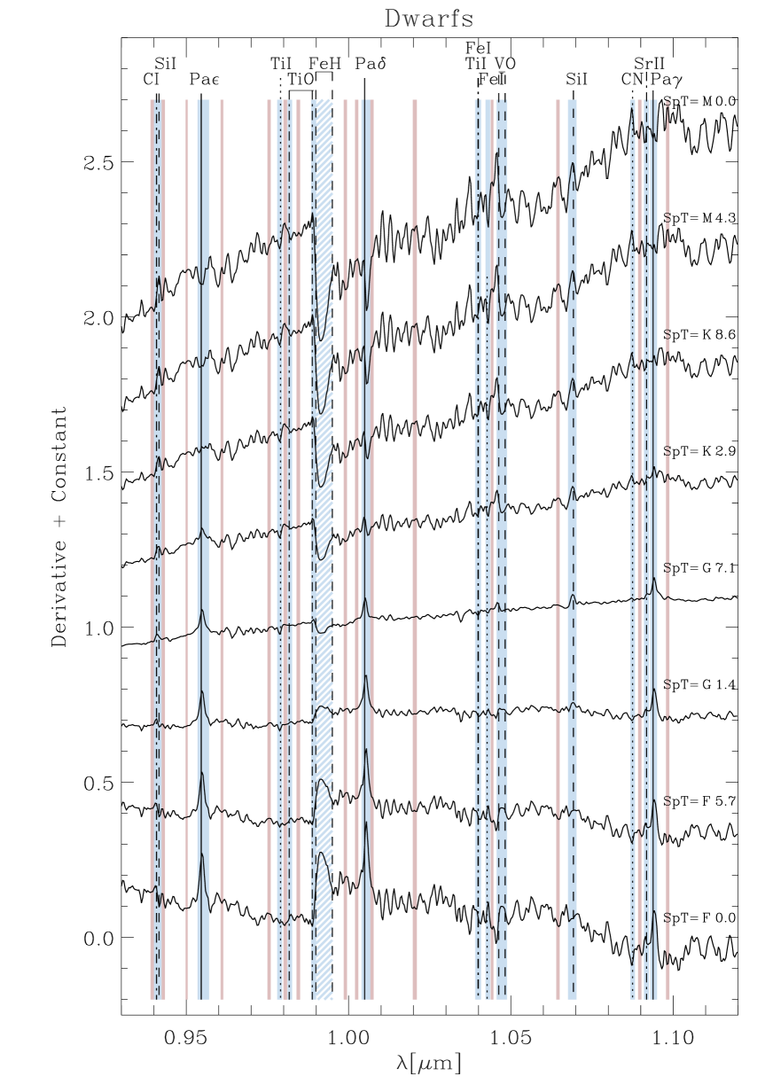
Figure 22: Y atmospheric window sensitivity map for SpT of dwarfs. Fig. 2 gives details.

The Y atmospheric sensitivity maps with respect to the SpTs are shown in Figs. 2, 21, and 22 for supergiant, giant, and dwarf stars, respectively.

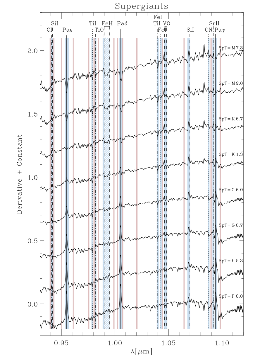
Figure 2: Y atmospheric window sensitivity map for SpT of supergiants. Details are given in Fig. 1. The plots for other luminosity classes and atmospheric windows are shown in Appendix A.

The regions corresponding to the Pa series of the H are sensitive to the spectral type, showing a positive peak for the F stars that gradually transforms into a negative peak for the M stars. A similar trend is also shown in the FeH region and, even if with less intensity, in the VO band. This behavior is more evident for dwarf than for supergiant and giant stars. The other elements show much weaker features in the sensitivity map (i.e., much weaker change in the spectrum). Si and Sr seem to be sensitive only for K and M stars, while the CN is very close to a Fe line and they are probably contaminating each other, introducing some instability into the trend.

The Y atmospheric sensitivity maps with respect to the surface gravity are shown in Figs. 3 and 4 for the F and G stars and K and M stars, respectively.

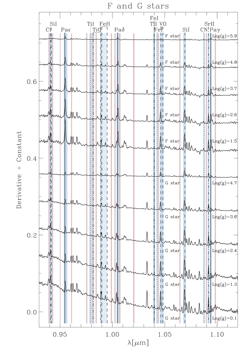
Figure 3: Y atmospheric window sensitivity map for surface gravity of F (top) and G-type stars (bottom). The sensitivities for different gravity values are offset for display purposes and the central values of the corresponding $\log{g}\,$bins are given. Figure 2 gives more details.

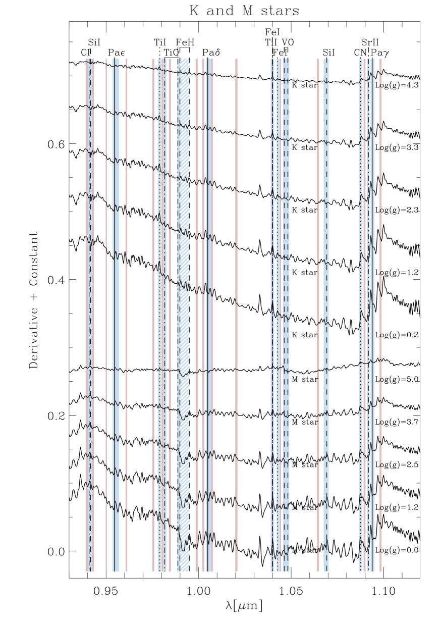
Figure 4: Y atmospheric window sensitivity map for surface gravity of K (top) and M-type stars (bottom). Figure 3 gives more details.

The lines of the Pa series of the H show a positive peak increasing from the low-gravity to high-gravity stars and being evident only for the G and F type stars. Some minor but significant changes have been found in the derivative plot of the Si and the Sr lines.

4.2 J atmospheric window

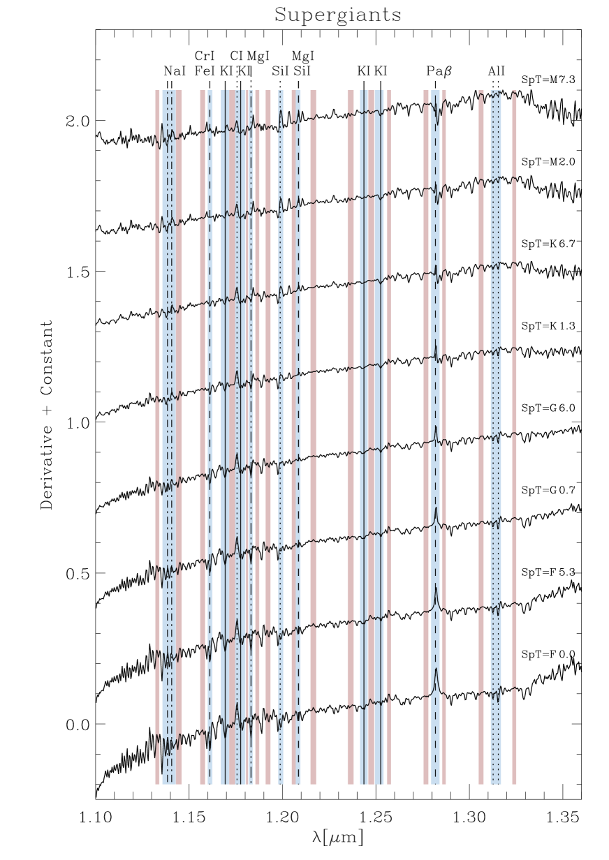
Figure 23: J atmospheric window sensitivity map for SpT of supergiants. Fig. 2 gives details.

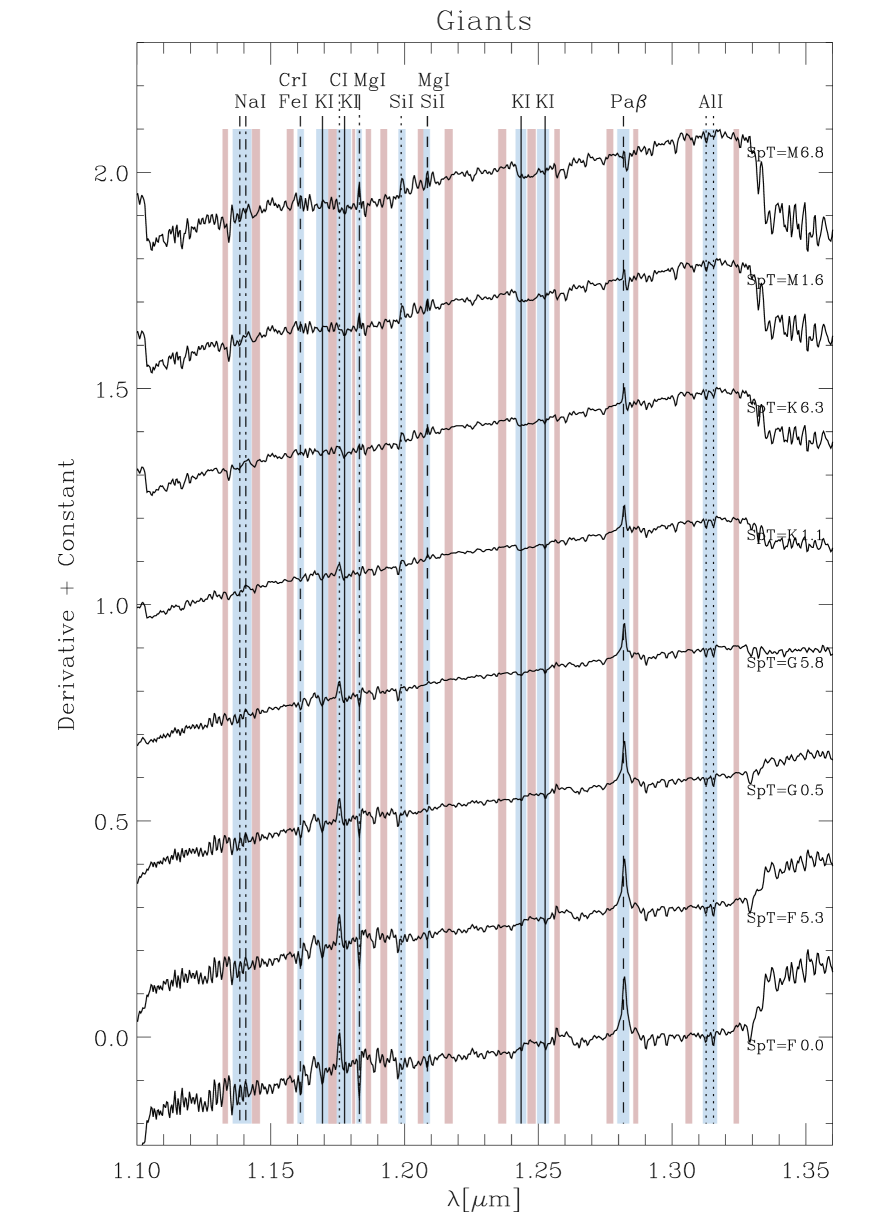
Figure 24: J atmospheric window sensitivity map for SpT of giants. Fig. 23 gives details.

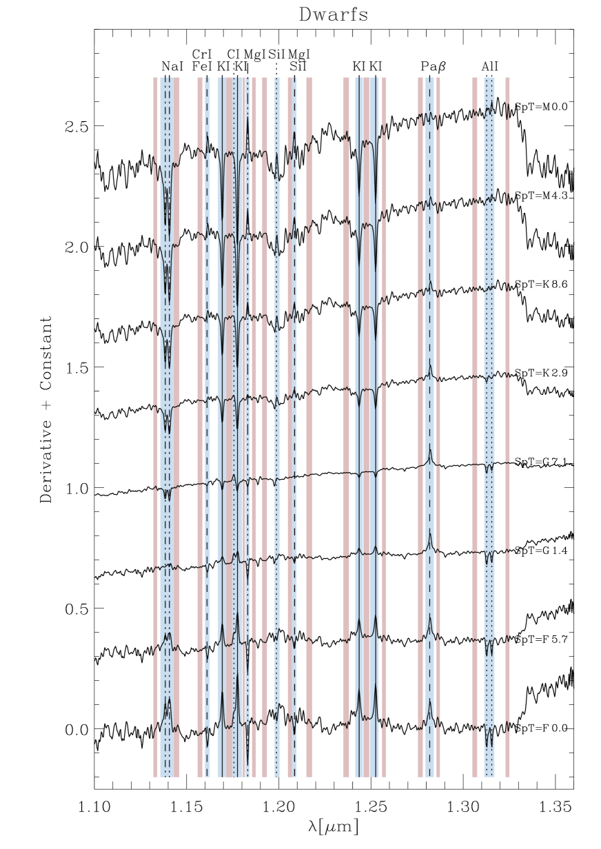
Figure 25: J atmospheric window sensitivity map for SpT of dwarfs. See Fig. 23 for details.

The J atmospheric sensitivity maps with respect to the SpTs are shown in Figs. 23, 24, and 25 for supergiant, giant, and dwarf stars, respectively. In this atmospheric window the behavior of supergiant and giant stars is different from that of the dwarf stars. The Na doublet, K, Mg, Si, and to a small extent Fe and Al show a very strong positive peak that decreases to very negative values moving from the early- to late-type dwarf stars. This trend is not visible for the supergiants and giant stars. In contrast, for supergiant and giant stars the most prominent features are Pa$\leavevmode\nobreak\ \beta$ and C with values that are positive for the F stars and decrease moving to the M stars. These changes are, instead, almost negligible for dwarf stars.

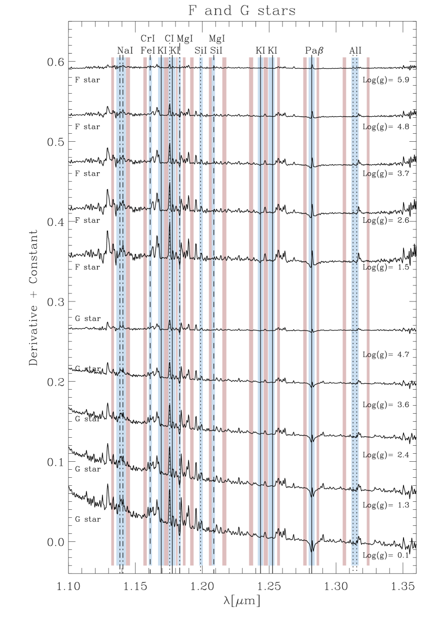
Figure 32: J atmospheric window sensitivity map for surface gravity of F- (top) and G-type stars (bottom). Fig. 3 gives details.

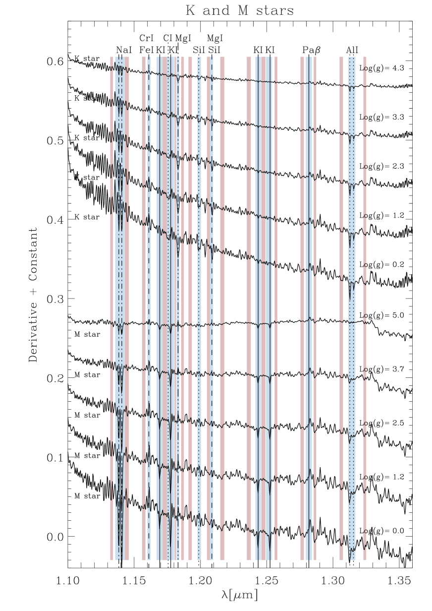
Figure 33: J atmospheric window sensitivity map for surface gravity of K- (top) and M-type stars (bottom). Fig. 4 gives details.

The J atmospheric sensitivity maps with respect to the surface gravity are shown in Figs. 32 and 33 for the F and G stars and K and M stars, respectively. Decreasing positive values from low-gravity to high-gravity stars for the C and Si elements were found in F and G stars, while Na and K elements show a dependence with gravity only in K and M stars.

4.3 H atmospheric window

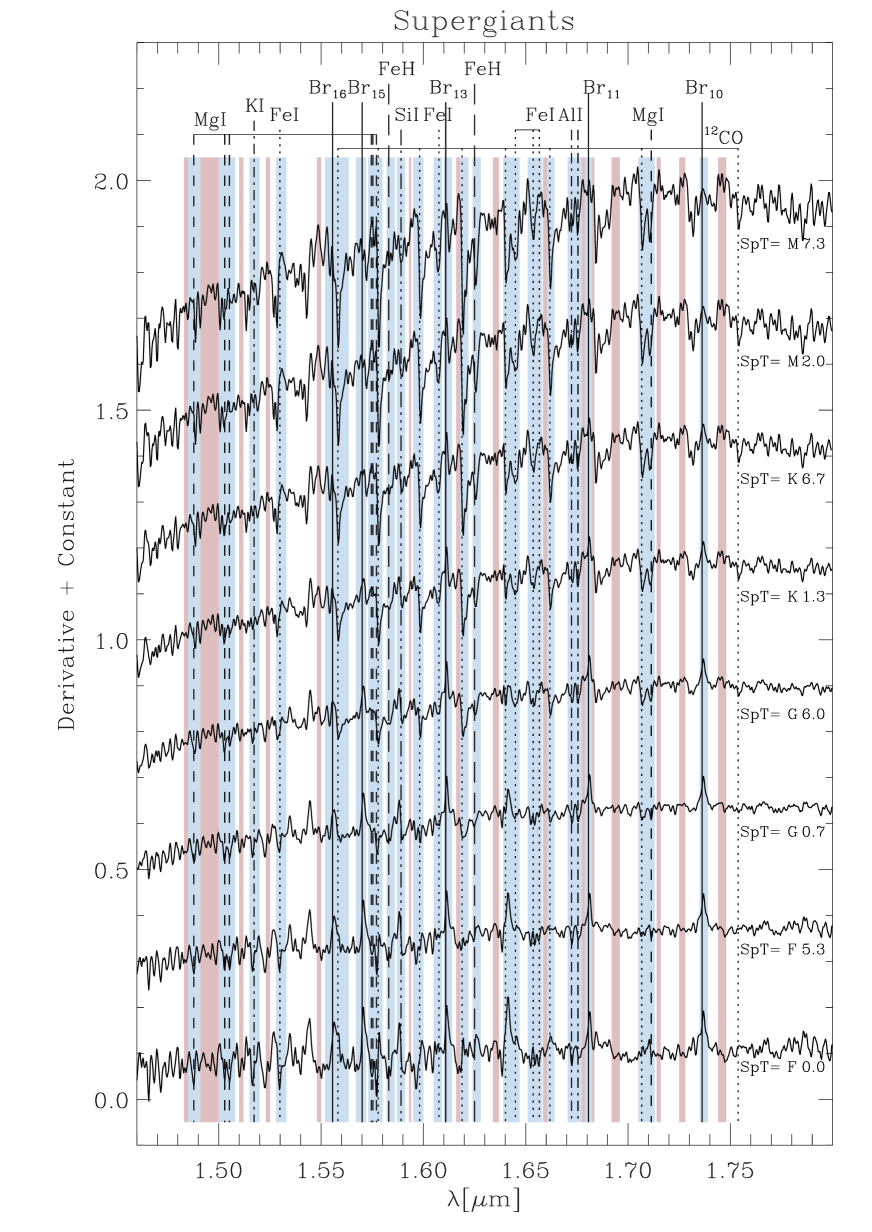
Figure 26: H atmospheric window sensitivity map for SpT of supergiants. ig. 2 gives details.

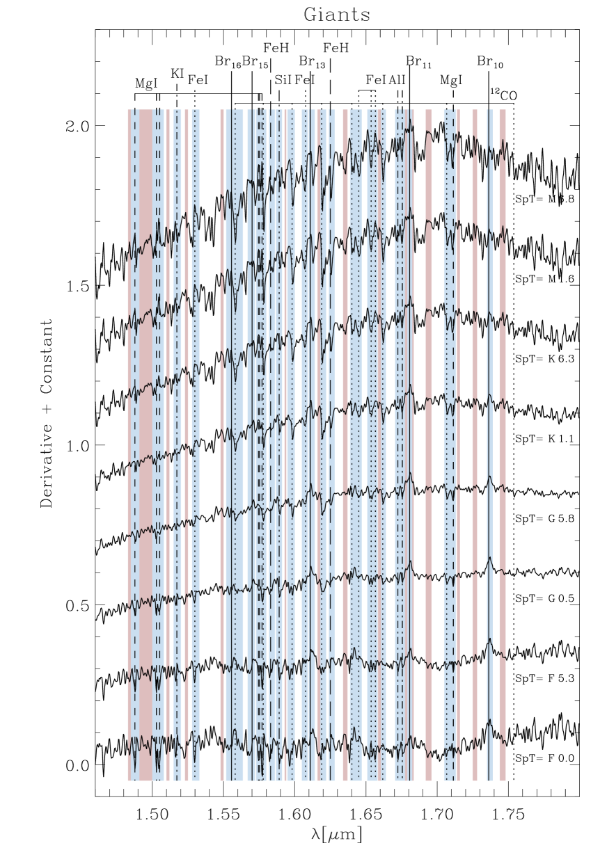
Figure 27: H atmospheric window sensitivity map for SpT of giants. Fig. 26 gives details.

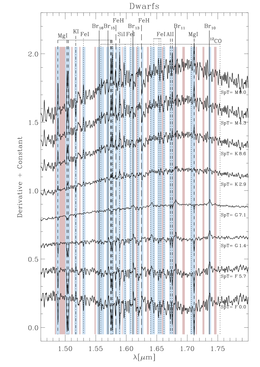
Figure 28: H atmospheric window sensitivity map for SpT of dwarfs. Fig. 26 gives details.

The H atmospheric sensitivity maps with respect to the SpTs are shown in Figs. 26, 27, and 28 for supergiant, giant, and dwarf stars, respectively. This is the atmospheric window with the strongest sensitivity, no matter which class of stars we consider. However, the elements showing sensitivity in giant and supergiant stars are different from the elements showing sensitivity for dwarf stars. For the latter the most evident changes are in the Mg, Si, Fe, and Al lines, while the Br lines do not display any significant peak. On the other hand, in sensitivity maps of the giant and supergiant stars the Br lines have a large range of variations, going from positive values in F stars to negative values in M stars. Even if less evident than in dwarf stars, the Mg, Si, Fe, and Al lines still maintain a weak sensitivity trend with the spectral type also in these classes.

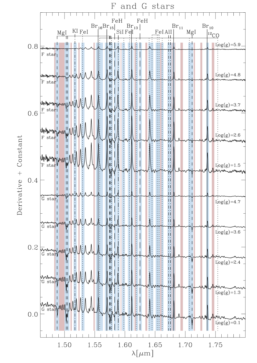
Figure 34: H atmospheric window sensitivity map for surface gravity of F- (top) and G-type stars (bottom). Fig. 3 gives details.

The H atmospheric sensitivity maps with respect to the surface gravity are shown in Figs. 34 and 35 for F and G stars and K and M stars, respectively. In the F and G stars the sensitivity maps show strong variations for the Br lines. Their peaks are always very positive indicating strong changes in the line width. The other elements have smaller variations not comparable with those of H lines but still detectable. Regarding the F and G stars, the dominant variations are detected in the Mg and CO lines, while the Br lines show minor variations.

4.4 L atmospheric window

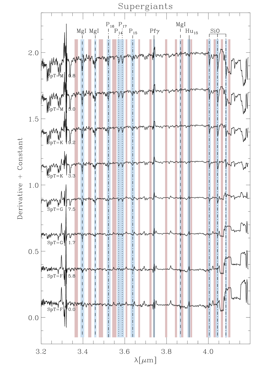
Figure 29: L atmospheric window sensitivity map for SpT of supergiants. See Fig. 2 for details.

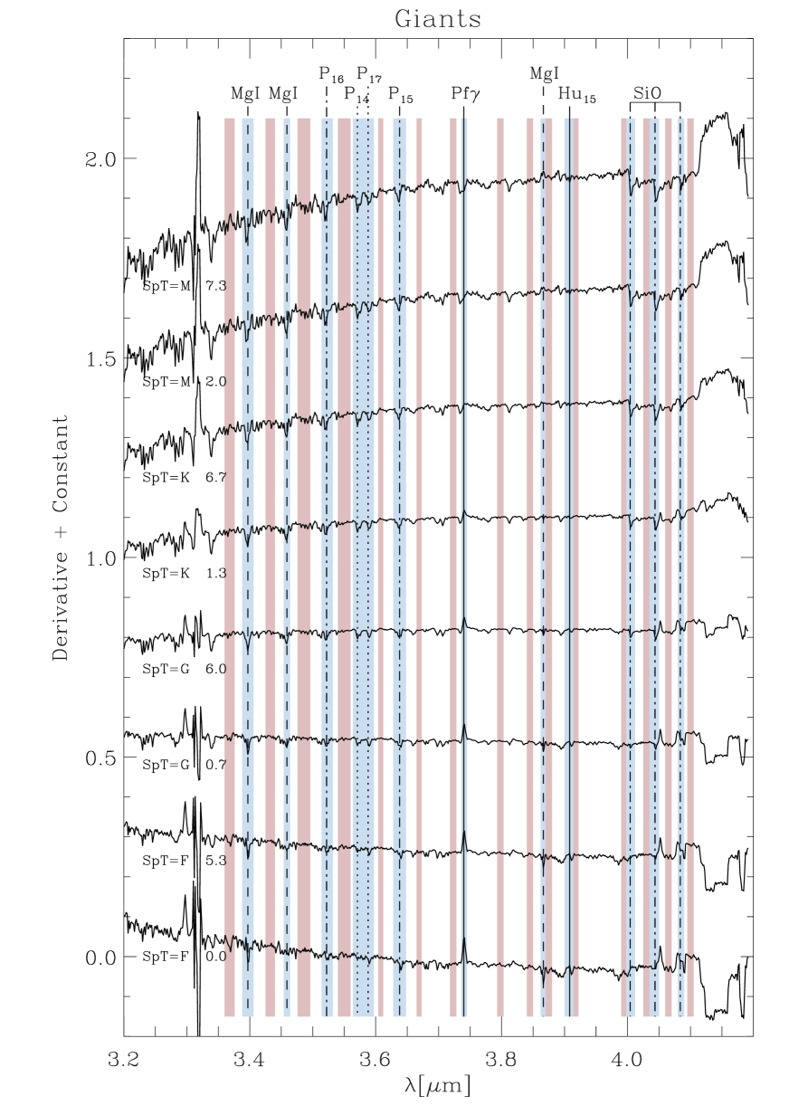
Figure 30: L atmospheric window sensitivity map for SpT of giants. Fig. 29 gives details.

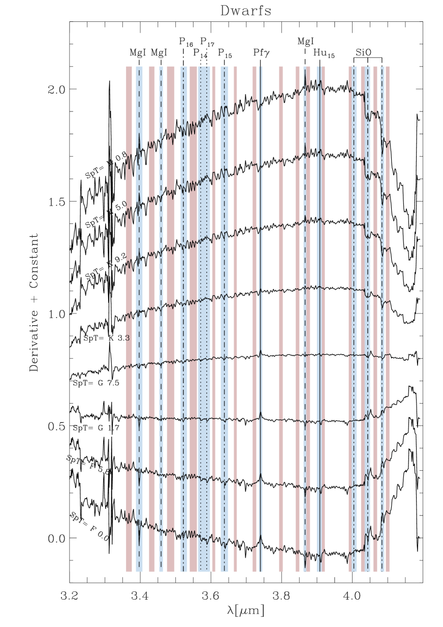
Figure 31: L atmospheric window sensitivity map for SpT of dwarfs. Fig. 29 gives details.

The L atmospheric sensitivity maps with respect to the SpTs are shown in Figs. 29, 30, and 31 for supergiant, giant, and dwarf stars, respectively. The most prominent feature is Mg, which decreases from the F to the M stars. For the Mg at $\lambda\simeq 3.4\,\mu$m we found a possible contamination that needs to be considered. The SiO also shows a clear peak in the sensitivity map decreasing from F stars to M stars. The P lines show medium to weak sensitivity to the changes along SpT.

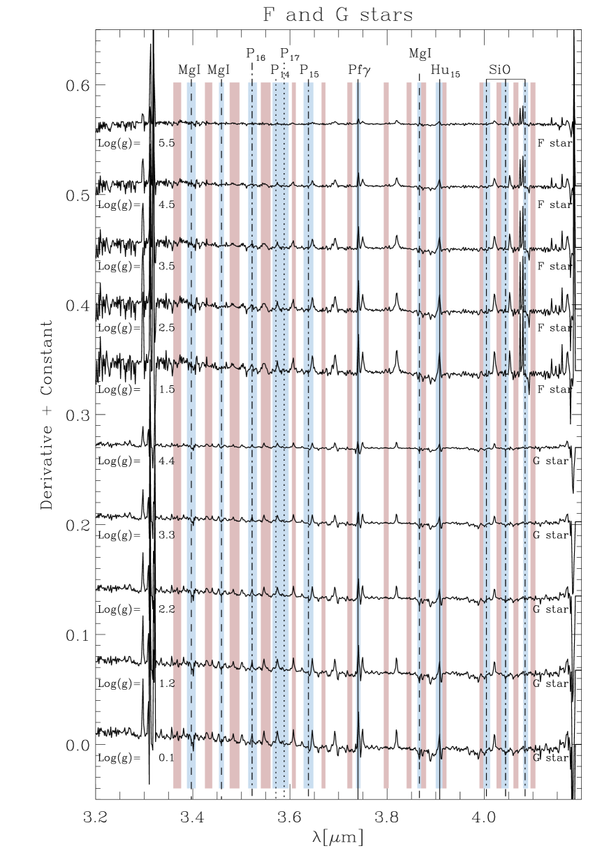
Figure 36: L atmospheric window sensitivity map for surface gravity of F- (top) and G-type stars (bottom). See Fig. 3 for details.

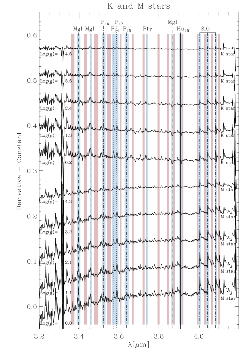
Figure 37: L atmospheric window sensitivity map for surface gravity of K- (top) and M-type stars (bottom). Fig. 4 gives details.

The L atmospheric sensitivity maps with respect to the surface gravity are shown in Figs. 36 and 37 for F and G stars and K and M stars, respectively. F and G stars show a weak dependency of the SiO lines with the surface gravity and almost no sensitivity has been detected in the sensitivity map of F and K stars.

5 Indices definition and equivalent width measurements

We defined an index for all the features that display a significant variation in the sensitivity maps (at least over some range of parameters), and that are therefore promising tools to measure $T_{\rm eff}\,$(or Spt) and $\log{g}\,$. For each index, we have a central bandpass covering the feature of interest and two adjacent bandpasses tracing the local “continuum” at the red and blue sides of the feature, as done in Paper I. The equivalent width for each spectral feature has been derived following Eq. 1 in Paper I. The central bandpass was designed to include the peak of the particular feature at the sensitivity map and the continuum bandpasses were placed on spectral regions where the sensitivity map is, as much as possible, constant.

We defined 14 indices in Y, 12 in J, 22 in H, and 12 in the L atmospheric windows. The index definitions are listed in Table 1 and their bandpasses are plotted in Figs. 1, 4, and 10–20. We measured the equivalent widths of all the indices. Their values are listed in Tables LABEL:tab:index_mis_Y_1 and LABEL:tab:index_mis_L_1 and plotted versus the star effective temperature and surface gravity in Figs. 8, 9, and 41–47, respectively.

The precision of the measured indices depends on the S/N ratio of the spectra, which varies widely because of the sky emission and telluric absorption features. To obtain a robust evaluation of the uncertainties of the indices, we simulated some indices of the Y band, choosing as example CSi, Pa$\epsilon$, and Pa$\delta$ for a FII star, Ti, CN, and Pa$\delta$ for a KIII star, and FeH, VO, and Pa$\delta$ for a MI star. We generated spectra with eight different S/N levels, ranging from 20 to 120, by adding artificial noise to the three test stars from the IRTF library.

Figure 5 shows the effect of the S/N on the precision of the measured indices. Generally, it is negligible except for very low S/N (¡10). For some features (e.g., Pa$\epsilon$ in FII star or FeH in MI star), we can obtain a precision of 10% for S/N$\sim$10-20, while for others (e.g., Pa$\delta$ in MI star or CN in KIII star) we can reach a precision of 30% for S/N$\sim$20-40. Only for a few weaker features, the precision remains at a 50% level even for higher S/N.

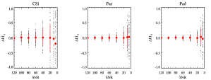
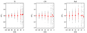
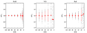
Figure 5: Deviation of the index (measured on the noisy artificial spectrum) from the index value in the “noiseless” spectrum, normalized by the latter, plotted versus the S/N of the noisy spectrum for Y band spectral features in MI (lower panels), KIII (central panels), and FII (upper panels) stars. The S/N is given per Å.

6 Sensitivity of indices to galaxy velocity dispersion broadening

The application of spectroscopic index systems to study stellar populations of unresolved galaxies (e.g., Dressler et al., 1987; Worthey et al., 1994b; Morelli et al., 2017) is affected by the intrinsic velocity dispersion that broadens the lines in the integrated spectra of the galaxies. This could render useless some weaker or close to each other indices that we defined in this work. It is therefore important to investigate how our measurements are affected by the internal kinematics of galaxies.

As done in Paper I and in order to take this into account, we broadened all the spectra by convolving them with a Gaussian of $\sigma$ varying from 115 to 400$\rm\,km\,s^{-1}$ in steps of 25$\rm\,km\,s^{-1}$. The indices were measured for all broadened spectra and a third-order polynomial fit was performed to the relative changes of each index $\Delta(Index)/Index(\sigma_{0})$ as a function of the velocity dispersion. As expected for our indices, we found a strong correlation between the line strength and broadening. The indices with a low equivalent width value show a large variation even for small values of $\sigma$ whereas the strongest indices are less affected.

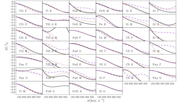
Figure 6: Sensitivity of the indices in the Y atmospheric window to the velocity dispersion broadening. The relative variations of indices $\Delta(Index)/Index(\sigma_{0})$ for different luminosity classes and spectral types are shown: supergiants with a black solid line, giants with a red dotted line, and dwarf stars with a violet dashed line.

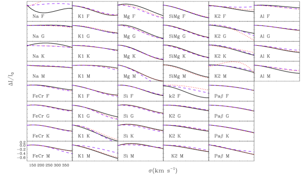
Figure 38: Sensitivity of the indices in the J atmospheric window to the velocity dispersion broadening. Fig. 6 gives details.

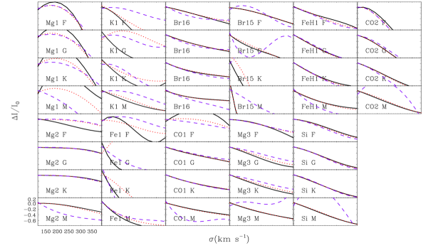
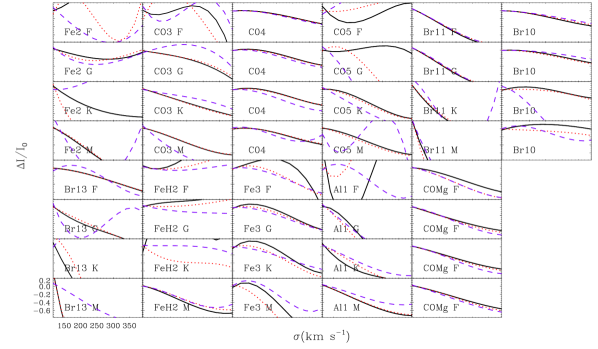
Figure 39: Sensitivity of the indices in the H atmospheric window to the velocity dispersion broadening. Fig. 6 gives details.

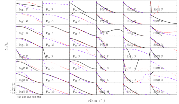
Figure 40: Sensitivity of the indices in the L atmospheric window to the velocity dispersion broadening. Fig. 6 gives details.

Figure 6 shows $\Delta(Index)/Index(\sigma_{0})$ versus the broadened velocity dispersion for the indices in the Y atmospheric window. The faintest indices are omitted here and in the subsequent figures. The results for indices in the J, H, and L windows are shown in Figs. 38,39, and 40, respectively.

To demonstrate the effect of broadening on the relations derived in Figs. 8, 41, 43, and 46, in Fig. 7 we show, as an example, the result of a different broadening in for Ti and Si versus the effective temperature (see Sect. 7 for details). We choose Ti and Si since they have a small and large scatter, respectively, in their correlation with the effective temperature. As expected, as the velocity dispersion increases, the broadening tends to reduce the trends and the equivalent widths flatten for a large velocity dispersion ($\sigma\geq 350$ $\rm km\;s^{-1}$), especially for Ti.

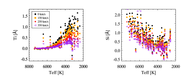
Figure 7: Effect of the velocity dispersion broadening on the $Ti-T_{eff}$ (left panel) and $Si-T_{eff}$ (right panel). With a black circle we show the original relation, and with a yellow square, red diamonds, and violet triangle the relation after a broadening of 150, 250, and 350 $\rm km\;s^{-1}$, respectively.

All indices and their correlation with the stellar properties are of course affected by the broadening effect at a different level depending on the spectral type, because lines may suffer from cross-contamination by different species in stars with different effective temperature. Without exhaustive discussion, we point out that the most reliable and stable indices over velocity dispersion ranging up to $\sim 200-250$ $\rm km\;s^{-1}$are CSi, Ti, and Pa$\delta$ in the Y atmospheric window, Na, FeCr, K1, Si, K2 and Pa$\beta$ in the J atmospheric window, Mg2, Mg3, Si, COMg, and Br₁₀ in the H atmospheric window, and Mg2 in the L atmospheric window.

7 Spectral diagnostics

The indices defined in Sect. 5 have dependencies on the stellar properties. In this section, we describe for each atmospheric window the behavior of the most relevant features presents.

7.1 Y atmospheric window

Almost all indices in the Y atmospheric window show some dependence on $T_{\rm eff}\,$, although with a different level of significance and over different temperature ranges (Fig. 8). For example, Pa$\epsilon$, Pa$\delta$, and Pa$\gamma$ indices are excellent temperature indicators for stars of types earlier than about G3. Other indices such as Ti, TiO A, TiO B, FeH, FeTi, Fe, and VO lines are complementary and work for the cooler stars. The Si, CN, and Sr indices are non-monotonic, which is also true to some extent for the Paschen indices. Finally, CSi has monotonic dependence over the almost entire range of interest, but this feature is relatively weak and shows some scatter.

The surface gravity is harder to infer from the Y window indices (Fig. 9, upper panels). Some molecular features related to TiO, FeH, VO, and CN do follow monotonic trends that are not strong in comparison with the measurement errors. The trends become more evident if the samples are constrained to a given spectral type, for example, to G type stars for the VO index or to M stars for the FeH index. A similar effect is seen with the metallicity. Indices such as CSi and TiO B show trends only when a certain luminosity class (like supergiant stars) is considered (Fig. 9, bottom panels).

7.2 J atmospheric window

Almost all the indices in the J window can serve as good $T_{\rm eff}$ indicators (Fig. 41). However, in most cases the trends in comparison with the scatter are relatively stronger than for the indices in the Y window. Notably in some cases, such as the K1A, K1B, K2A, and K2B indices, the trends for stars of different luminosity classes are identical. This allows us to estimate the stellar temperature without information about the luminosity class. The dwarf stars cooler than mid-M type show an extremely strong $T_{\rm eff}$ dependence for many indices, including Na, K1A, C, K1B, Si, K2A, and K2B. However, this is due to contamination by molecules such as methane. These indices reach values in the dwarf stars that are not measured in the stars of other luminosity classes, making it obvious that the stars are dwarf. There are no indices that show degeneracy, with the exception of Mg and Al only for dwarf stars.

Some J window indices can serve as luminosity indicators. They are FeCr, K1A, K1B, and Si. Na, K2A, and Al are useful if only certain spectral types are considered (Fig. 42, upper panels). The K1A index appears to be by far the best one, and more notably it shows the same behavior over the entire range of spectral types. Disappointingly, none of the J window indices seem to correlate with [Fe/H], and Mg- and Fe-dominated indices need further investigation (Fig. 42, bottom panels).

7.3 H atmospheric window

The indices in the H atmospheric window in general show a more complex behavior than those in the Y and J windows (Figs. 43 and 43). The dwarf stars show non-monotonic behavior more often than not and there are no indices with identical trends for supergiant, giant, and dwarf stars, except for some spectral classes, for example, CO1, CO2, CO3, FeH1, and FeH2 for stars earlier than K0, and COMg for stars earlier than K7. However, the different behavior of some indices in stars of different luminosity classes can be used to our advantage to separate the luminosity classes. For example, various CO-based indices have very different values for dwarf stars, as long as they are cooler than mid-K or early-M types. This diagnostic can be brought to stars as hot as early-K for FeH2 and CO5 indices, and as early as G with the help of the Mg1 and Mg2 indices provided there are no metallicity effects. This behavior is clearly visible in Fig. 44.

Br₁₀, Si, and CO4 indices are shown to be very promising $\log{g}\,$indicators in the H window (Fig. 44). None of the investigated indices here show significant metallicity trend (Fig. 45). Unfortunately, the Mg feature at $\lambda\simeq 1.58\,\mu$m is severely contaminated with other lines and it seems to be rather temperature sensitive at $\lambda\simeq 1.71\,\mu$m, (Le et al., 2011). The passband of Si at $\lambda\simeq 1.596\,\mu$m includes the strong line of Fe $\lambda\simeq 1.599\,\mu$m, which is also increasing with decreasing effective temperature. These effect requires further investigation but this will be possible only after widening the metallicity range of the library stars.

7.4 L atmospheric window

The L window is relatively devoid of spectral features in comparison with the other windows. We see the same variety of behavior with respect to the temperature as in the other windows (Fig. 46). The Pf$\gamma$ index appears to be the best temperature indicator for stars earlier than G2 and various indices encompassing the OH band for the cooler stars. The same OH-based indices together with the SiO-based indices can help to separate dwarfs from giants and supergiant stars for spectral types later than K3. However, the intrinsic scatter of the relations for L window indices is larger than for the indices in the other atmospheric windows – not surprising given the stronger thermal background at $\lambda>$2.5 $\mu$m.

The index with the most consistent behaviour with respect to the surface gravity across all the spectral types is Hu₁₅ (Fig. 47, upper panels), although to be reliable diagnostics the S/N of the data is critical. Like the previous cases, we found no significant correlations with [Fe/H] (Fig. 47, bottom panels).

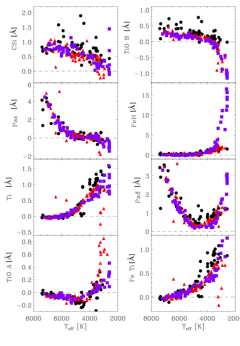
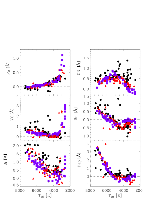
Figure 8: Index measurements in the Y atmospheric window as functions of effective temperature. The different symbols correspond to the supergiants (circles), giants (triangles), and dwarf stars (squares), respectively.

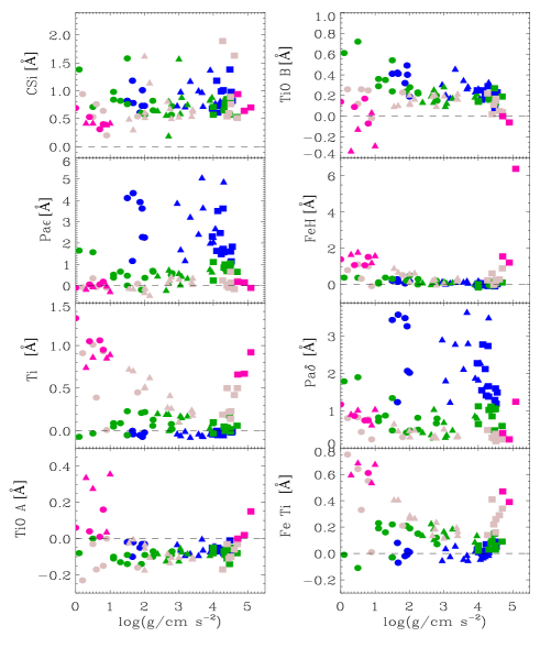
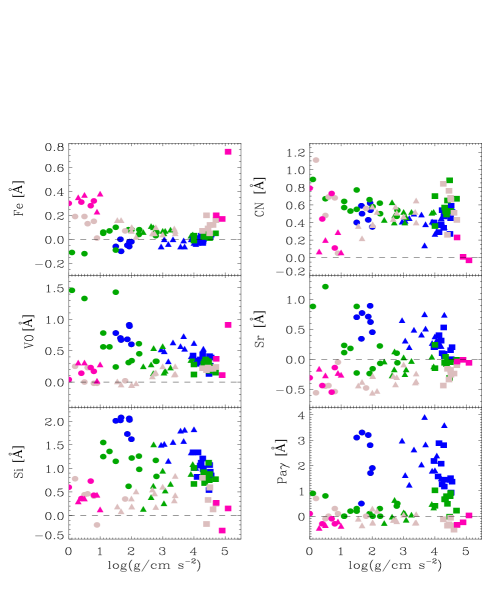
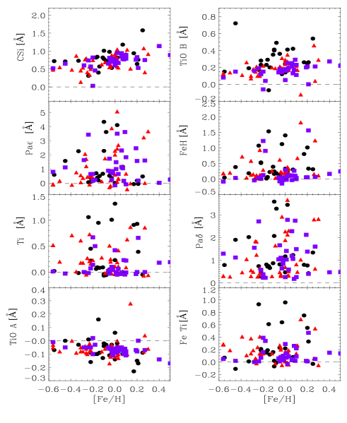
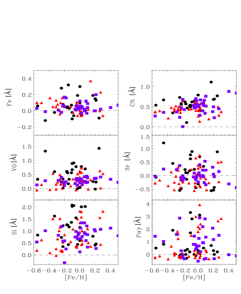
Figure 9: Index measurements in the Y atmospheric window as functions of surface gravity (top panels) and metallicity (bottom panels). Symbols for supergiants, giants, and dwarf stars are as in Fig. 8. Different colors in the top panels correspond to F (blue), G (green), K (gray), and M type stars (pink), respectively.

8 Discussion and summary

The analysis presented here is based on stellar spectra. We relate the strengths of various spectral features with the physical properties of the stars – effective temperature $T_{\rm eff}\,$, surface gravity $\log{g}\,$, and metallicity [Fe/H]. However, our main goal is to relate the strengths of these spectral features to the physical parameters of stellar populations in unresolved galaxies, and we adopt a simple and straightforward mapping of one to the other. The temperature $T_{\rm eff}\,$is related to the population age, because the luminosity-weighted temperature decreases as the population passively evolves from being dominated by younger main-sequence stars towards older red giant stars. The surface gravity $\log{g}\,$tells us what is the dominant luminosity class of a population. Finally, the metallicity [Fe/H] translates into the cumulative abundance of the dominant population in a galaxy. We will investigate these diagnostics in a forthcoming paper (Gasparri et al. 2020, submitted) by measuring them in the sample of galaxies observed with X-Shooter (François et al., 2019). Furthermore, we will also compare the observational behavior of our defined indices with the predictions from the theoretical models (e.g., Röck et al., 2016; Conroy et al., 2018).

We point out that the diagnostics described here can also be used for spectral typing of individual stars. Last but not least, we stress that the behavior of the indices is not necessarily the same as the behavior of the particular species that dominate these indices, because of the possible contamination by other species as noted also by Conroy & van Dokkum (2012) in their models analyzing the initial mass function indicators. For example, some hydrogen and metal lines are contaminated by molecular bands in the late-type giant and supergiant stars.

To summarize, we present here an analysis of stellar spectra in the Y, J, H, and L atmospheric windows, based on high-quality medium resolution ($R\sim 2000-2500$) spectra of more than 200 stars with almost solar metallicity ($-0.5\leq$ [Fe/H]$\leq 0.5$ dex) and a spectral S/N of about 100 (Rayner et al., 2009). We identify the best indicators for the different stellar physical parameters, and as discussed above, of some integrated parameters of the stellar populations in unresolved galaxies. The results discussed in Sect. 7 have been summarized in Table 2.

Table 2: Summary of the best indicators for the different stellar physical parameters. For the details, please refer to Sect. 7. The columns show the following: (1) stellar physical parameters (2) spectral feature (3) quality of the index: strong (S) or weak (W) (4): notes on the index.

Stellar parameters	Index	Quality	Notes
(1)	(2)	(3)	(4)
Y atmospheric windows
$T_{\rm eff}$	Pa$\epsilon$,Pa$\delta$,Pa$\gamma$	S	F, G stars
	Ti,TiO A,TiO B,FeH,FeTi,Fe, VO	S	G, K, M stars
	CSi	W	Stars of all spectral type
$\log{g}\,$	TiO,FeH,VO,CN	S/W	Very dependent on star spectral type
[Fe/H]	TiO B	S	Only in supergiant stars
J atmospheric windows
$T_{\rm eff}$	K1 B,K2 A,K2 B	S	Similar trend in stars of all spectral types
	K1 A,Na,Si	S	M stars, methane contamination
$\log{g}\,$	FeCr,K1 B,Na,Si,Al	S	Dependent on star spectral type
	K1 A	S	All spectral type stars
H atmospheric windows
$T_{\rm eff}$	CO1,CO2,CO3,FeH1,FeH2,COMg	S	Mostly in F,G stars
$\log{g}\,$	Br10,Si,CO4	S	Stars of all spectral types
L atmospheric windows
$T_{\rm eff}$	Pf$\gamma$	W	In stars earlier than G2
$\log{g}\,$	Mg3,Hu15	W	Stars of all spectral type

Features sensitive to the effective temperature are present and measurable in all the investigated atmospheric windows. The surface gravity is more challenging: the H window offers better tools for a separation between dwarf and giant stars, followed by the J window. This is almost impossible in the Y and L windows. The diagnostics in the L window are the most challenging because the spectra are typically noisier than in other windows due to the higher thermal background emission. However, the next generation of both extremely large ground-based telescopes and space-based facilities will work in this regime, making even these L window diagnostic tools quite valuable.

Appendix A Main spectral features plots

The model spectra in Y, J, H and L atmospheric windows for stars of different luminosity classes are shown in Figs. 1 and 10–20.

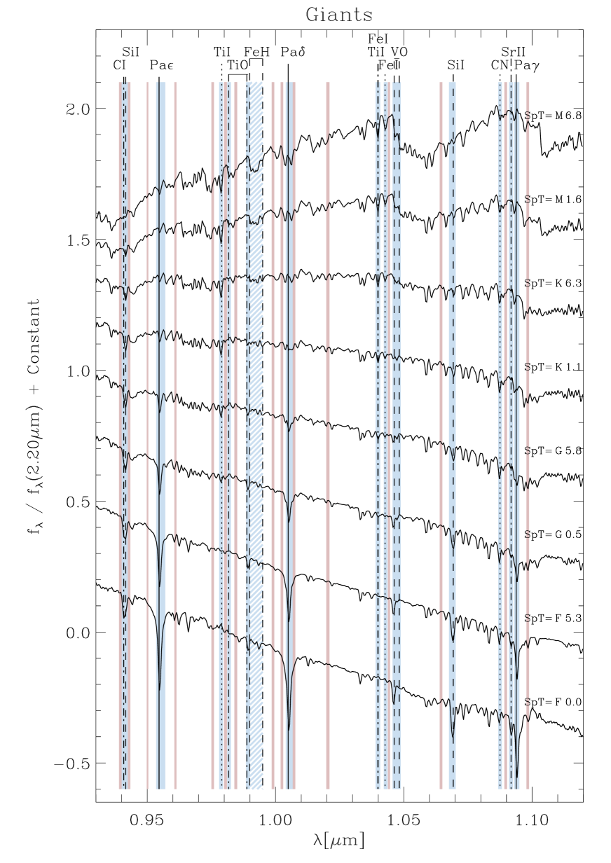
Figure 10: Y atmospheric window model spectrum of giants. Figure 1 gives details.

Figure 11: Y atmospheric window model spectrum of dwarfs. Figure 1 gives details.

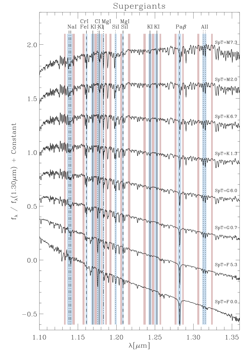
Figure 12: $J$ atmospheric window model spectrum of supergiants. The flux-normalization here is performed at 1.30$\,\mu$m. Figure 1 gives details.

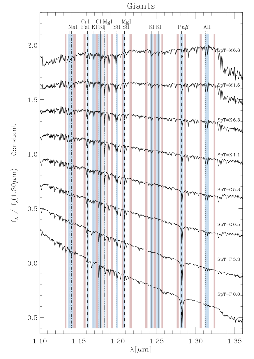
Figure 13: $J$ atmospheric window model spectrum of giants. Figure 12 gives details.

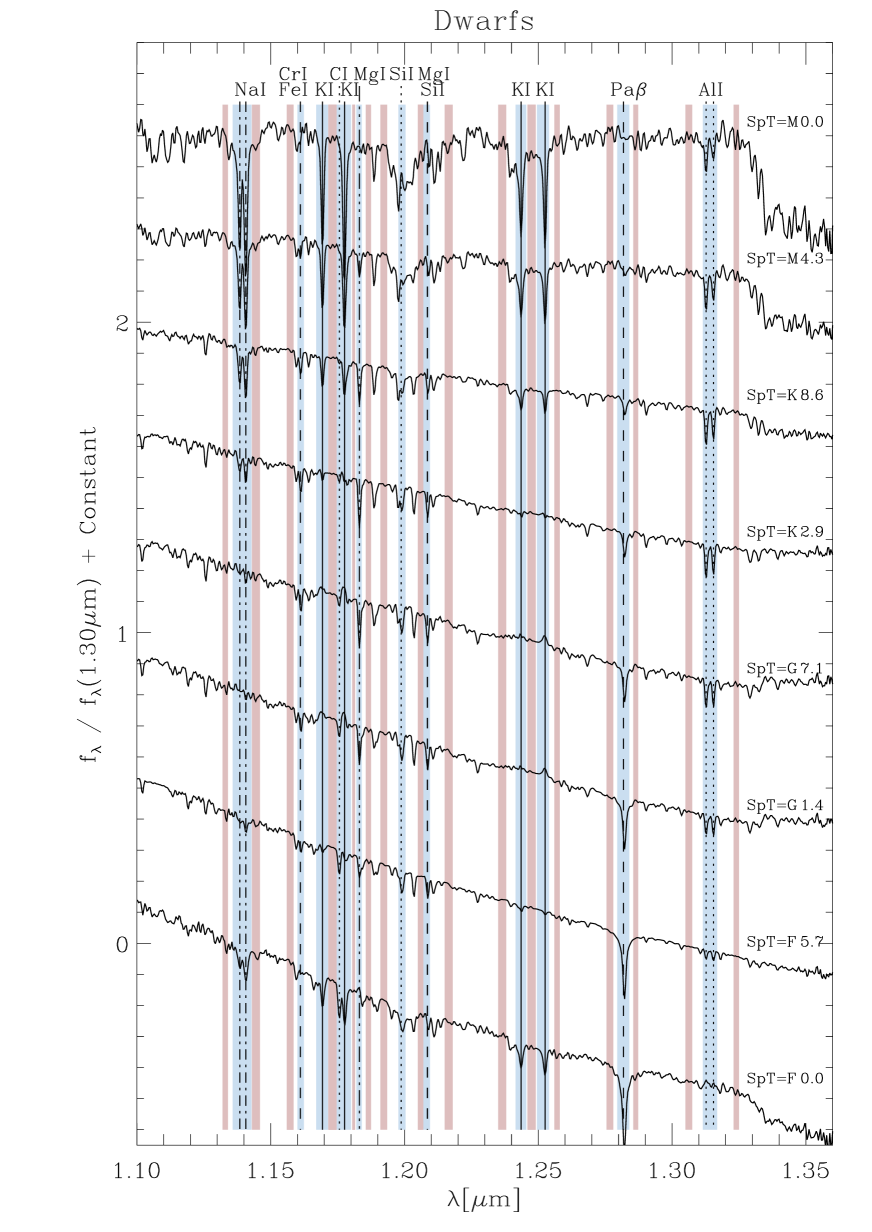
Figure 14: $J$ atmospheric window model spectrum of dwarfs. Figure 12 gives details.

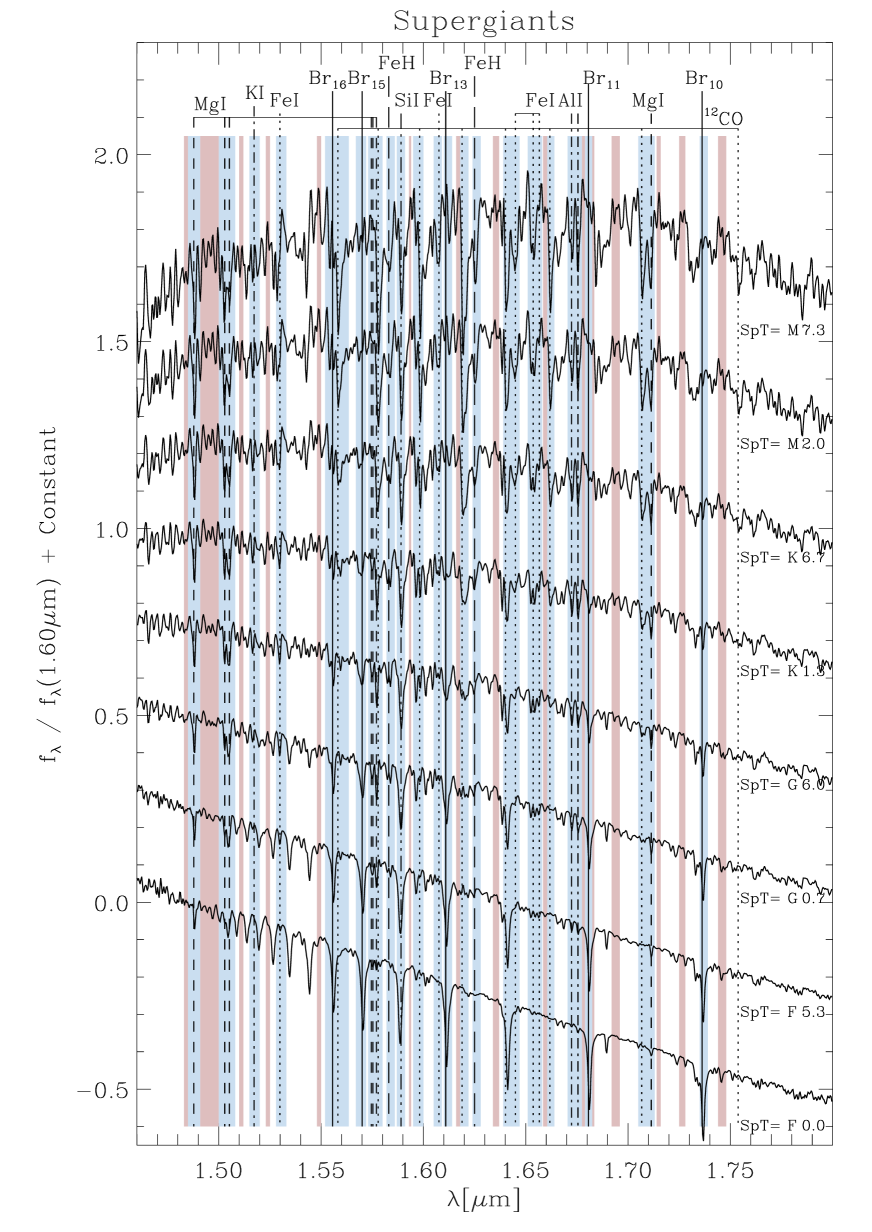
Figure 15: H window model spectrum of supergiants. The flux-normalization here is performed at 1.60$\,\mu$m. Figure 1 gives details.

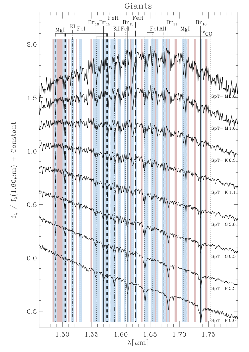
Figure 16: H window model spectrum of giants. Figure 15 gives details.

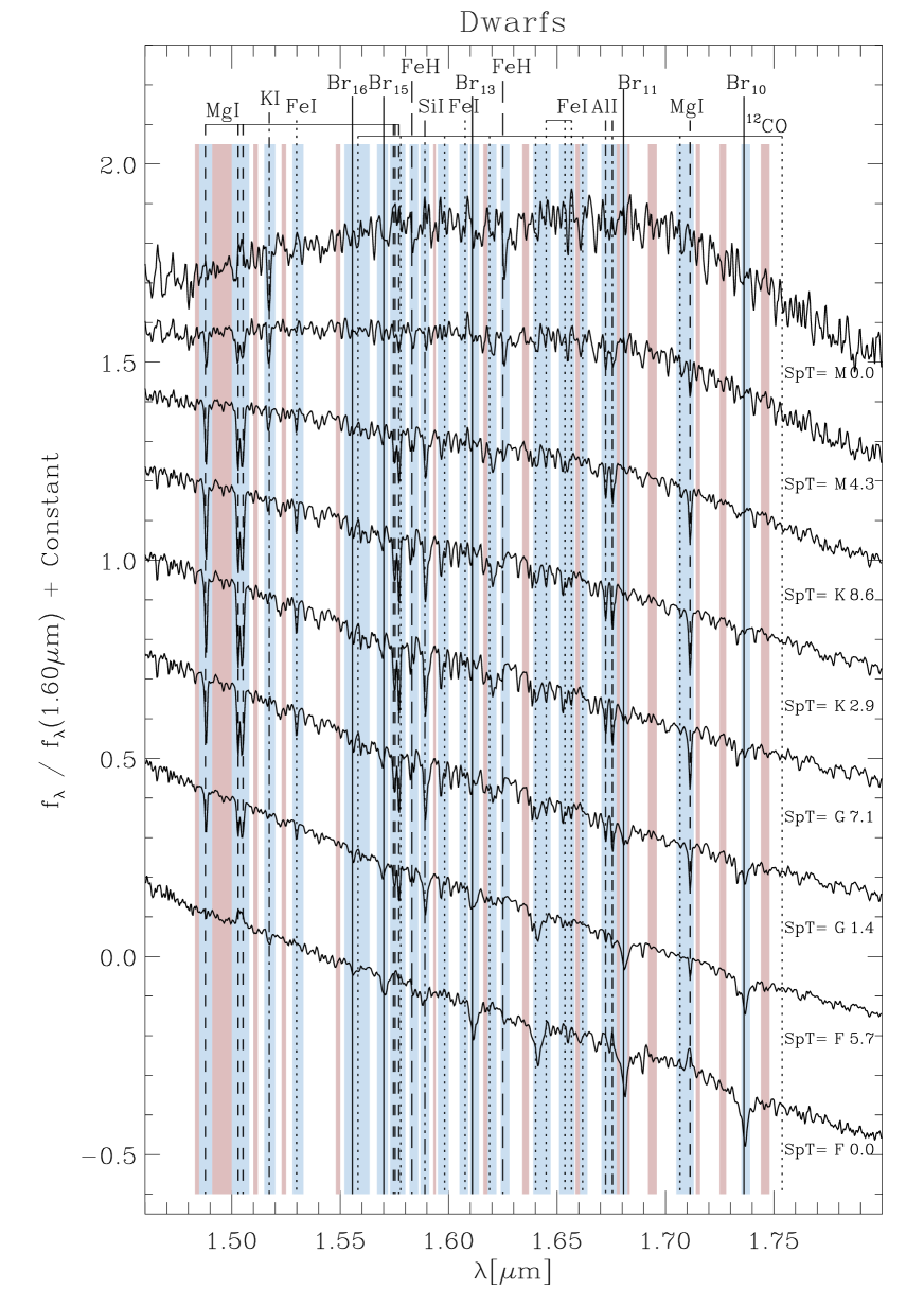
Figure 17: H window model spectrum of dwarfs. Figure 15 gives details.

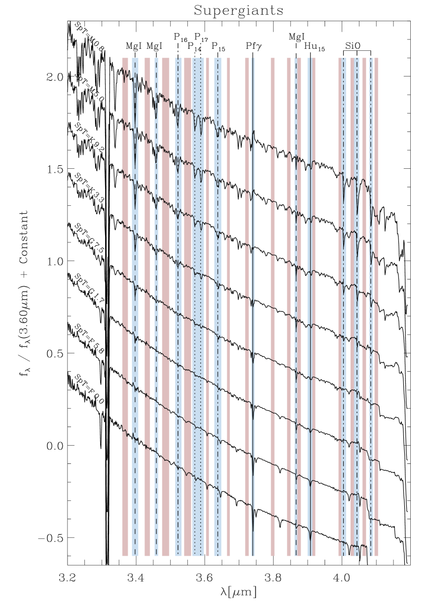
Figure 18: L atmospheric window model spectrum of supergiants. The flux-normalization here is performed at 3.60$\,\mu$m. Figure 1 gives details.

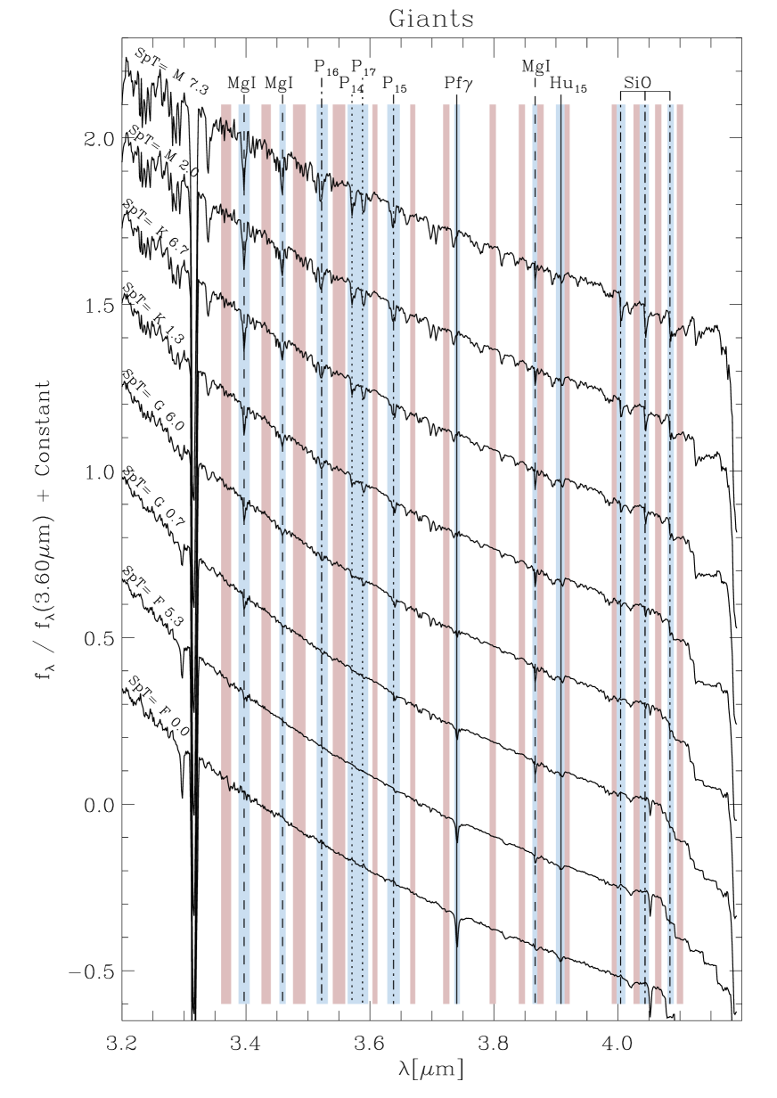
Figure 19: L atmospheric window model spectrum of giants. Figure 18 gives details.

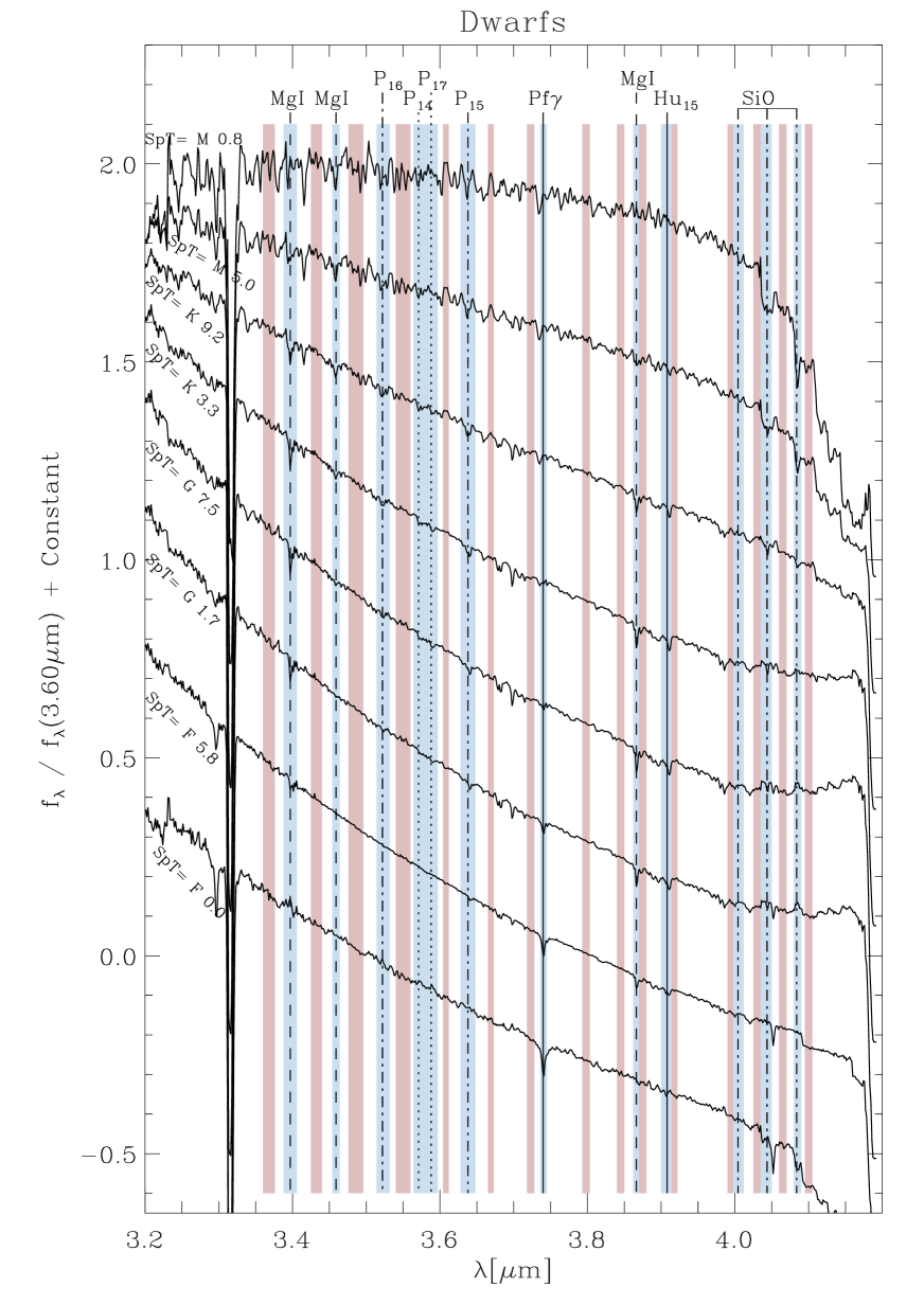
Figure 20: L atmospheric window model spectrum of dwarfs. Figure 18 gives details.

Appendix B Sensitivity map plots

The sensitivity maps for SpT in J, H, and L atmospheric windows for stars of different luminosity classes are shown in Figs. 2 and 21–20. The corresponding sensitivity maps for surface gravity in Y, J, H, and L atmospheric windows for stars of different luminosity classes are shown in Figs. 2 and 21–20.

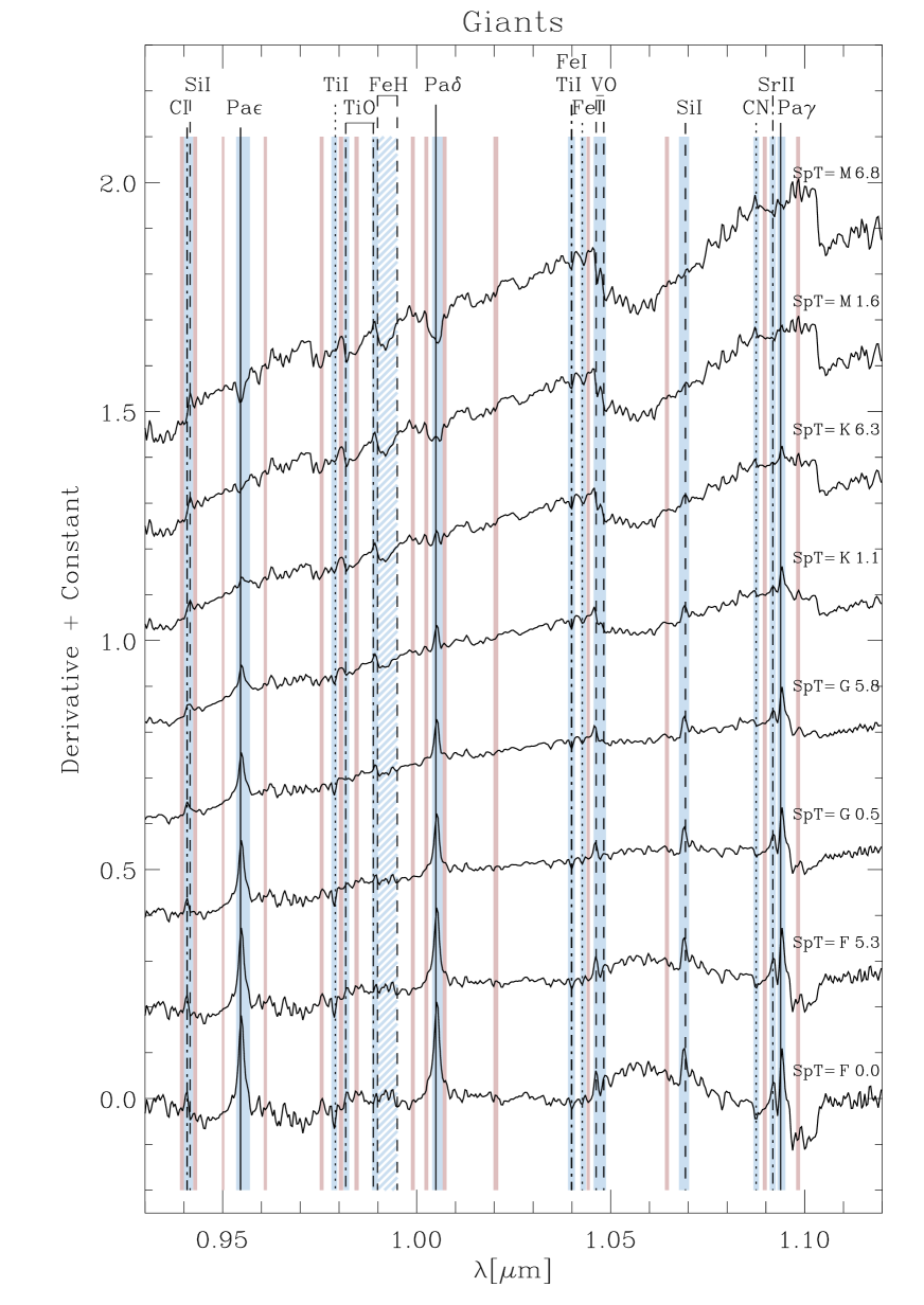
Figure 21: Y atmospheric window sensitivity map for SpT of giants. Fig. 2 gives details.

Figure 35: H atmospheric window sensitivity map for surface gravity of K- (top) and M-type stars (bottom). Fig. 4 gives details.

Appendix C Broadening effects

Appendix D Behavior of the spectral indices

The behavior of index measurements in the Y, J, H, and L atmospheric window as functions of effective temperature, surface gravity and metallicity for stars of different luminosity classes are shown in Figs. 8, 9, and 41–47.

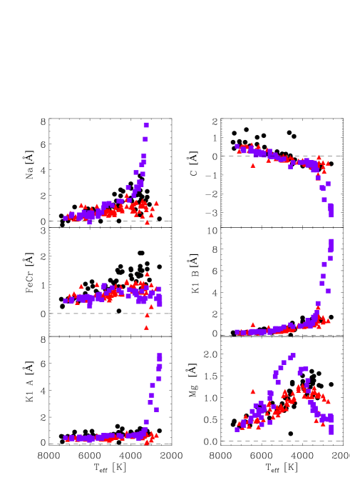
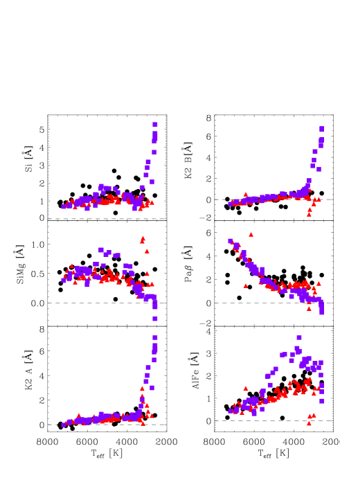
Figure 41: Index measurements in the J atmospheric window as functions of effective temperature. For details see Fig. 8.

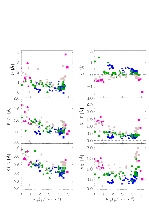
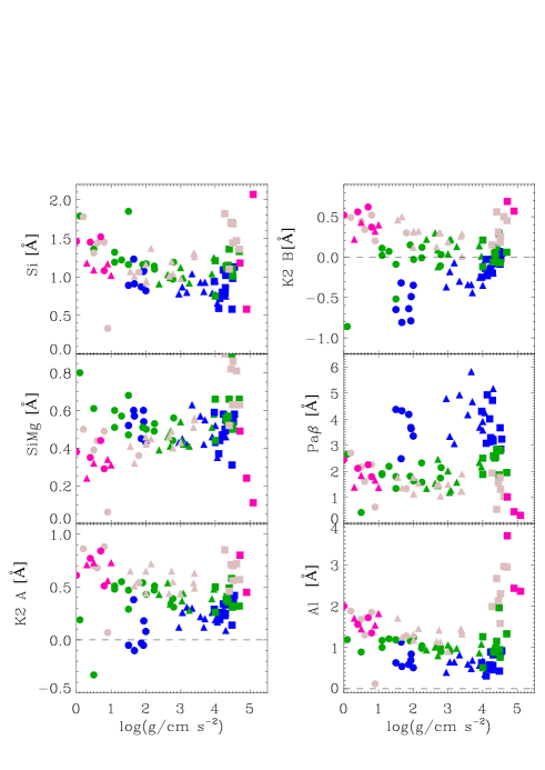
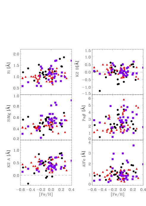
Figure 42: Index measurements in the J atmospheric window as functions of surface gravity (top panels) and metallicity (bottom panels). For details see Fig. 9.

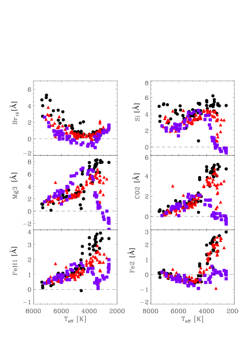
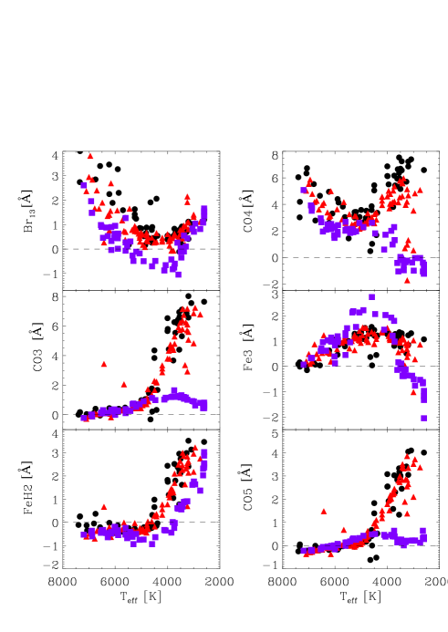
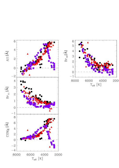
Figure 43: Index measurements in the H atmospheric window as functions of effective temperature. For details see Fig. 8.

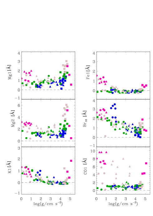
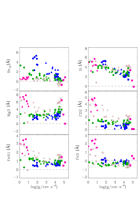
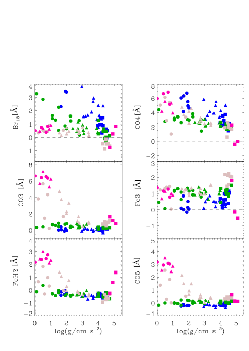
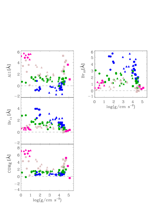
Figure 44: Index measurements in the H atmospheric window as functions of surface gravity. For details see Fig. 9.

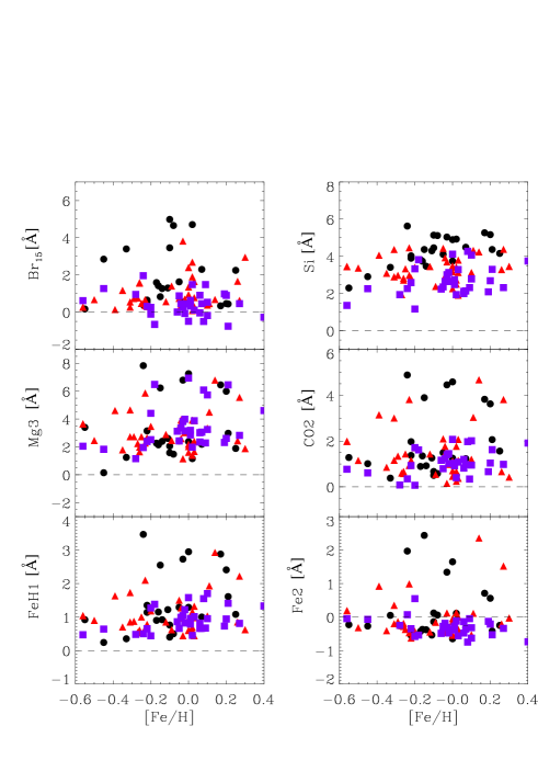
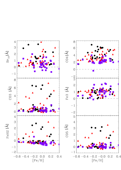
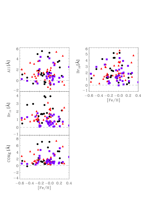
Figure 45: Index measurements in the H atmospheric window as functions of metallicity. For details see Fig. 9.

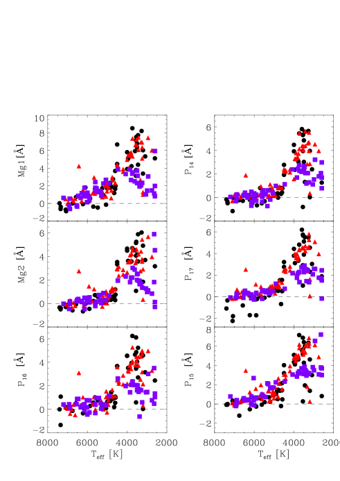
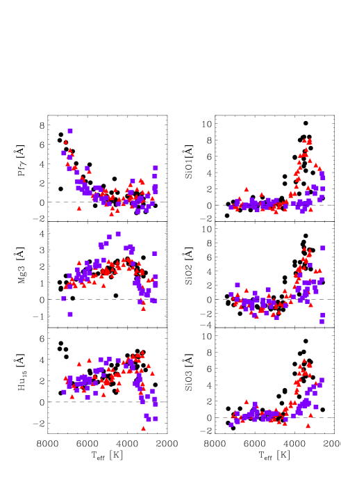
Figure 46: Index measurements in the L atmospheric window as functions of effective temperature. For details see Fig. 8.

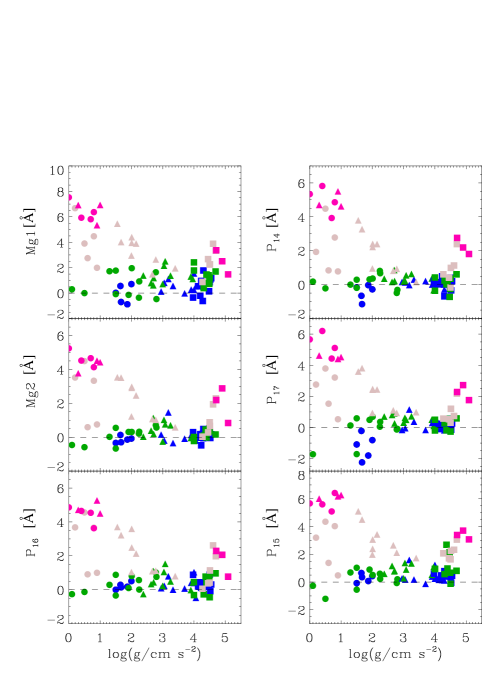
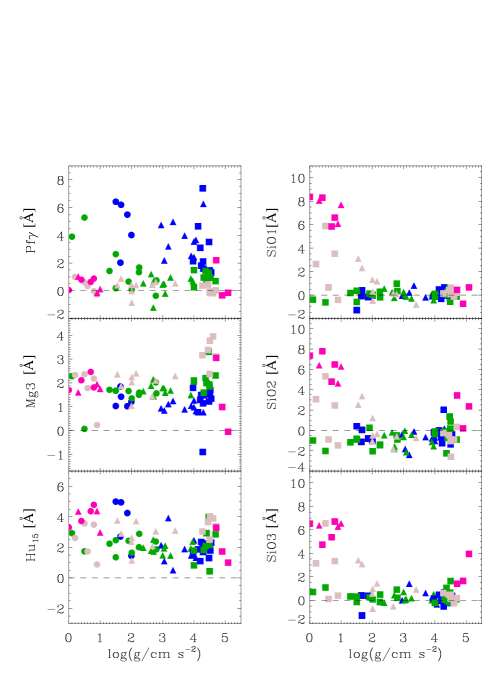
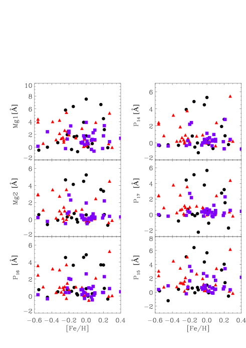
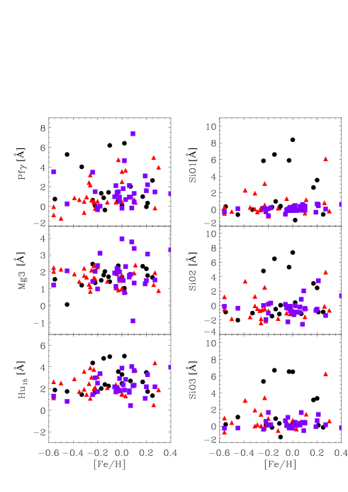
Figure 47: Index measurements in the L atmospheric window as functions of surface gravity (top panels) and metallicity (bottom panels). For details see Fig. 8.

Appendix E Equivalent width tables

In this section we report values measured for all the indices in the different bands. The tables are just an example and their integral version will be published in the online material.

Table 3: Equivalent widths of the $Y$-band indices. Part A.

Star IDs	CSi	Pa$\epsilon$	Ti	TiO A	TiO B	FeH	Pa$\delta$	FeTi	Fe
Supergiants
HD007927	0.74 $\pm$ 0.06	3.07 $\pm$0.65	0.03 $\pm$0.01	0.03 $\pm$ 0.01	0.56 $\pm$0.01	0.49 $\pm$0.02	2.92 $\pm$0.03	-0.05 $\pm$0.03	-0.05 $\pm$0.03
HD006130	0.82 $\pm$ 0.05	4.11 $\pm$0.46	-0.05 $\pm$0.03	-0.02 $\pm$ 0.02	0.41 $\pm$0.01	0.22 $\pm$0.03	3.44 $\pm$0.08	-0.03 $\pm$0.07	-0.06 $\pm$0.07
HD135153	0.61 $\pm$ 0.13	3.92 $\pm$0.46	-0.05 $\pm$0.03	-0.05 $\pm$ 0.03	0.32 $\pm$0.02	0.07 $\pm$0.05	3.49 $\pm$0.07	-0.02 $\pm$0.05	-0.05 $\pm$0.05
HD173638	0.78 $\pm$ 0.07	4.34 $\pm$0.42	-0.04 $\pm$0.01	-0.02 $\pm$ 0.02	0.41 $\pm$0.01	0.16 $\pm$0.04	3.58 $\pm$0.10	-0.07 $\pm$0.05	-0.10 $\pm$0.05
…	…	…	…	…	…	…	…	…	…
Giants
HD089025	0.89 $\pm$ 0.01	3.89 $\pm$ 0.25	-0.03 $\pm$ 0.02	-0.03 $\pm$ 0.02	0.31 $\pm$ 0.01	0.19 $\pm$ 0.03	2.92 $\pm$ 0.08	-0.05 $\pm$ 0.06	-0.06 $\pm$ 0.06
HD027397	0.68 $\pm$ 0.02	4.89 $\pm$ 0.21	-0.05 $\pm$ 0.02	-0.06 $\pm$ 0.02	0.33 $\pm$ 0.01	0.09 $\pm$ 0.03	3.51 $\pm$ 0.10	-0.01 $\pm$ 0.03	-0.01 $\pm$ 0.03
HD013174	0.92 $\pm$ 0.01	3.67 $\pm$ 0.23	-0.06 $\pm$ 0.01	-0.06 $\pm$ 0.02	0.29 $\pm$ 0.01	0.11 $\pm$ 0.04	2.82 $\pm$ 0.09	-0.05 $\pm$ 0.04	-0.06 $\pm$ 0.04
HD40535	0.89 $\pm$ 0.02	3.49 $\pm$ 0.22	-0.05 $\pm$ 0.02	-0.04 $\pm$ 0.02	0.30 $\pm$ 0.01	0.05 $\pm$ 0.02	2.68 $\pm$ 0.08	-0.02 $\pm$ 0.03	-0.02 $\pm$ 0.03
…	…	…	…	…	…	…	…	…	…
Dwarfs
HD108519	0.73 $\pm$ 0.04	4.45 $\pm$ 0.21	-0.03 $\pm$ 0.01	-0.02 $\pm$ 0.01	0.24 $\pm$ 0.02	0.11 $\pm$ 0.05	3.30 $\pm$ 0.09	-0.03 $\pm$ 0.03	-0.02 $\pm$ 0.03
HD213135	0.74 $\pm$ 0.04	3.43 $\pm$ 0.20	-0.02 $\pm$ 0.01	-0.05 $\pm$ 0.01	0.19 $\pm$ 0.00	0.04 $\pm$ 0.01	2.71 $\pm$ 0.08	0.01 $\pm$ 0.03	-0.02 $\pm$ 0.03
HD113139	0.95 $\pm$ 0.02	3.50 $\pm$ 0.22	-0.05 $\pm$ 0.02	-0.05 $\pm$ 0.01	0.25 $\pm$ 0.01	0.09 $\pm$ 0.03	2.78 $\pm$ 0.09	-0.03 $\pm$ 0.02	-0.03 $\pm$ 0.02
HD026015	0.89 $\pm$ 0.03	3.62 $\pm$ 0.18	-0.05 $\pm$ 0.02	-0.06 $\pm$ 0.02	0.29 $\pm$ 0.01	0.10 $\pm$ 0.04	2.74 $\pm$ 0.09	0.02 $\pm$ 0.03	-0.03 $\pm$ 0.03
…	…	…	…	…	…	…	…	…	…

Table 4: Equivalent widths of the $Y$-band indices. Part B.

Star IDs	VO	Si	CN	Sr	Pa$\gamma$
Supergiants
HD007927	0.87 $\pm$0.04	3.26 $\pm$0.02	0.51 $\pm$ 0.02	1.00 $\pm$0.01	2.56 $\pm$0.02
HD006130	0.78 $\pm$0.09	2.01 $\pm$0.02	0.40 $\pm$ 0.01	0.70 $\pm$0.03	3.11 $\pm$0.06
HD135153	0.68 $\pm$0.06	1.73 $\pm$0.02	0.43 $\pm$ 0.01	0.71 $\pm$0.03	3.18 $\pm$0.07
HD173638	0.67 $\pm$0.08	2.08 $\pm$0.03	0.50 $\pm$ 0.03	0.77 $\pm$0.03	3.29 $\pm$0.06
…	…	…	…	…	…
Giants
HD089025	0.52 $\pm$ 0.11	1.50 $\pm$ 0.03	0.41 $\pm$ 0.03	0.65 $\pm$ 0.03	2.98 $\pm$ 0.08
HD027397	0.53 $\pm$ 0.06	1.04 $\pm$ 0.03	0.35 $\pm$ 0.02	0.74 $\pm$ 0.01	3.59 $\pm$ 0.03
HD013174	0.53 $\pm$ 0.06	1.82 $\pm$ 0.04	0.38 $\pm$ 0.03	0.51 $\pm$ 0.02	2.83 $\pm$ 0.05
HD40535	0.65 $\pm$ 0.05	1.49 $\pm$ 0.02	0.37 $\pm$ 0.02	0.51 $\pm$ 0.01	2.70 $\pm$ 0.03
…	…	…	…	…	…
Dwarfs
HD108519	0.43 $\pm$ 0.04	1.61 $\pm$ 0.01	0.06 $\pm$ 0.01	0.51 $\pm$ 0.01	3.40 $\pm$ 0.03
HD213135	0.40 $\pm$ 0.05	1.19 $\pm$ 0.02	0.24 $\pm$ 0.02	0.37 $\pm$ 0.01	2.86 $\pm$ 0.02
HD113139	0.34 $\pm$ 0.03	1.34 $\pm$ 0.02	0.29 $\pm$ 0.02	0.40 $\pm$ 0.02	2.88 $\pm$ 0.05
HD026015	0.44 $\pm$ 0.03	1.21 $\pm$ 0.02	0.34 $\pm$ 0.02	0.53 $\pm$ 0.03	2.80 $\pm$ 0.08
…	…	…	…	…	…

Table 5: Equivalent widths of the $J$-band indices.

Star IDs	Na	FeCr	FeK	C	K	Mg	Si	SiMg	KMg	CrK	Pab	Al
Supergiants
HD007927	-0.01 $\pm$ 0.30	0.26 $\pm$ 0.03	0.55 $\pm$ 0.07	1.22 $\pm$ 1.44	0.17 $\pm$ 0.04	0.46 $\pm$ 0.06	0.73 $\pm$ 0.01	0.33 $\pm$ 0.02	-0.22 $\pm$ 0.09	-0.79 $\pm$ 0.19	2.36 $\pm$ 0.03	0.52 $\pm$ 0.02
HD006130	0.40 $\pm$ 0.24	0.50 $\pm$ 0.02	0.58 $\pm$ 0.05	0.74 $\pm$ 1.46	0.25 $\pm$ 0.04	0.38 $\pm$ 0.06	0.89 $\pm$ 0.01	0.52 $\pm$ 0.04	-0.05 $\pm$ 0.06	-0.65 $\pm$ 0.17	4.37 $\pm$ 0.07	0.63 $\pm$ 0.02
HD135153	0.02 $\pm$ 0.36	0.52 $\pm$ 0.04	0.53 $\pm$ 0.09	0.61 $\pm$ 1.60	0.21 $\pm$ 0.05	0.34 $\pm$ 0.06	0.87 $\pm$ 0.02	0.45 $\pm$ 0.04	-0.03 $\pm$ 0.07	-0.64 $\pm$ 0.17	4.18 $\pm$ 0.07	0.59 $\pm$ 0.07
HD173638	0.27 $\pm$ 0.30	0.43 $\pm$ 0.03	0.58 $\pm$ 0.05	0.78 $\pm$ 1.50	0.19 $\pm$ 0.03	0.34 $\pm$ 0.05	0.91 $\pm$ 0.02	0.57 $\pm$ 0.04	-0.10 $\pm$ 0.09	-0.81 $\pm$ 0.22	4.32 $\pm$ 0.06	0.54 $\pm$ 0.03
…	…	…	…	…	…	…	…	…	…	…	…	…
Giants
HD089025	0.62 $\pm$ 0.18	0.50 $\pm$ 0.01	0.52 $\pm$ 0.02	0.51 $\pm$ 1.52	0.17 $\pm$ 0.03	0.31 $\pm$ 0.05	0.78 $\pm$ 0.02	0.43 $\pm$ 0.04	0.12 $\pm$ 0.03	-0.37 $\pm$0.11	4.79 $\pm$ 0.07	0.40 $\pm$ 0.02
HD027397	0.41 $\pm$ 0.19	0.48 $\pm$ 0.02	0.34 $\pm$ 0.05	0.26 $\pm$ 1.68	0.20 $\pm$ 0.02	0.40 $\pm$ 0.02	0.75 $\pm$ 0.01	0.46 $\pm$ 0.02	0.09 $\pm$ 0.03	-0.19 $\pm$0.06	5.17 $\pm$ 0.11	0.46 $\pm$ 0.03
HD013174	0.25 $\pm$ 0.22	0.61 $\pm$ 0.02	0.54 $\pm$ 0.05	0.51 $\pm$ 1.55	0.37 $\pm$ 0.03	0.41 $\pm$ 0.02	0.93 $\pm$ 0.02	0.55 $\pm$ 0.04	0.20 $\pm$ 0.03	-0.44 $\pm$0.09	4.67 $\pm$ 0.05	0.69 $\pm$ 0.02
HD40535	0.36 $\pm$ 0.20	0.47 $\pm$ 0.01	0.51 $\pm$ 0.03	0.51 $\pm$ 1.51	0.21 $\pm$ 0.02	0.36 $\pm$ 0.03	0.82 $\pm$ 0.01	0.43 $\pm$ 0.02	0.20 $\pm$ 0.02	-0.30 $\pm$0.07	4.48 $\pm$ 0.08	0.47 $\pm$ 0.01
…	…	…	…	…	…	…	…	…	…	…	…	…
Dwarf
HD108519	0.22 $\pm$ 0.20	0.44 $\pm$ 0.02	0.47 $\pm$ 0.04	0.52 $\pm$ 1.65	0.30 $\pm$0.02	0.26 $\pm$ 0.02	0.69 $\pm$ 0.01	0.38 $\pm$ 0.04	-0.04 $\pm$ 0.04	-0.45 $\pm$ 0.09	5.26 $\pm$ 0.12	0.43 $\pm$ 0.02
HD213135	0.39 $\pm$ 0.19	0.43 $\pm$ 0.01	0.43 $\pm$ 0.03	0.38 $\pm$ 1.55	0.24 $\pm$0.03	0.38 $\pm$ 0.03	0.71 $\pm$ 0.01	0.41 $\pm$ 0.03	0.15 $\pm$ 0.03	-0.19 $\pm$ 0.07	4.87 $\pm$ 0.08	0.44 $\pm$ 0.02
HD113139	0.54 $\pm$ 0.14	0.49 $\pm$ 0.02	0.51 $\pm$ 0.04	0.37 $\pm$ 1.49	0.25 $\pm$0.02	0.36 $\pm$ 0.02	0.72 $\pm$ 0.01	0.44 $\pm$ 0.03	0.19 $\pm$ 0.03	-0.23 $\pm$ 0.07	4.93 $\pm$ 0.09	0.49 $\pm$ 0.03
HD026015	0.50 $\pm$ 0.17	0.50 $\pm$ 0.01	0.39 $\pm$ 0.03	0.29 $\pm$ 1.59	0.26 $\pm$0.01	0.44 $\pm$ 0.03	0.79 $\pm$ 0.01	0.50 $\pm$ 0.04	0.23 $\pm$ 0.03	-0.20 $\pm$ 0.06	4.72 $\pm$ 0.10	0.53 $\pm$ 0.01
…	…	…	…	…	…	…	…	…	…	…	…	…

Table 6: Equivalent widths of the $H$-band indices. Part A.

Star IDs	Mg1	Mg2	K1	Fe1	Br16	CO1	Br15	Mg3	FeH1	HMg	CO2S ts
Supergiants
HD007927	0.34 $\pm$ 0.55	1.20 $\pm$0.60	1.40 $\pm$0.07	0.08 $\pm$ 0.09	3.07 $\pm$ 0.11	0.69 $\pm$ 0.12	4.01 $\pm$ 0.02	0.56 $\pm$ 0.22	0.10 $\pm$ 0.12	3.74 $\pm$ 0.17	0.66 $\pm$ 0.09
HD006130	0.38 $\pm$ 0.13	0.90 $\pm$0.32	0.60 $\pm$0.06	0.06 $\pm$ 0.15	3.07 $\pm$ 0.25	0.95 $\pm$ 0.26	4.71 $\pm$ 0.03	1.16 $\pm$ 0.49	0.48 $\pm$ 0.26	4.93 $\pm$ 0.37	0.50 $\pm$ 0.11
HD135153	0.31 $\pm$ 0.17	0.84 $\pm$0.32	0.65 $\pm$0.06	0.13 $\pm$ 0.15	3.47 $\pm$ 0.23	1.27 $\pm$ 0.24	5.28 $\pm$ 0.04	1.70 $\pm$ 0.46	0.45 $\pm$ 0.25	5.23 $\pm$ 0.35	0.22 $\pm$ 0.14
HD173638	0.30 $\pm$ 0.18	1.04 $\pm$0.37	0.84 $\pm$0.07	0.07 $\pm$ 0.18	3.31 $\pm$ 0.31	1.01 $\pm$ 0.32	4.99 $\pm$ 0.03	1.58 $\pm$ 0.61	0.40 $\pm$ 0.32	5.14 $\pm$ 0.46	0.50 $\pm$ 0.11
…	…	…	…	…	…	…	…	…	…	…	…
Giants
HD089025	0.34 $\pm$ 0.08	0.65 $\pm$0.23	0.09 $\pm$ 0.03	0.01 $\pm$0.12	1.49 $\pm$ 0.22	0.54 $\pm$ 0.22	3.82 $\pm$ 0.04	1.15 $\pm$ 0.42	0.44 $\pm$ 0.23	3.70 $\pm$0.33	0.15 $\pm$ 0.17
HD027397	0.49 $\pm$ 0.08	0.71 $\pm$0.26	0.04 $\pm$ 0.04	0.05 $\pm$0.09	1.02 $\pm$ 0.16	0.63 $\pm$ 0.16	2.37 $\pm$ 0.04	1.62 $\pm$ 0.30	0.49 $\pm$ 0.16	2.46 $\pm$0.24	0.23 $\pm$ 0.15
HD013174	0.53 $\pm$ 0.10	0.89 $\pm$0.31	0.09 $\pm$ 0.04	-0.01 $\pm$0.09	1.39 $\pm$ 0.15	0.80 $\pm$ 0.16	2.95 $\pm$ 0.03	1.88 $\pm$ 0.30	0.62 $\pm$ 0.16	3.46 $\pm$0.23	0.42 $\pm$ 0.12
HD40535	0.42 $\pm$ 0.08	0.83 $\pm$0.29	0.02 $\pm$ 0.04	0.01 $\pm$0.14	1.08 $\pm$ 0.24	0.55 $\pm$ 0.25	2.84 $\pm$ 0.05	1.58 $\pm$ 0.47	0.49 $\pm$ 0.25	2.99 $\pm$0.37	0.28 $\pm$ 0.21
…	…	…	…	…	…	…	…	…	…	…	…
Dwarfs
HD108519	0.40 $\pm$0.06	0.65 $\pm$ 0.22	-0.00 $\pm$0.02	0.03 $\pm$ 0.06	1.08 $\pm$ 0.09	0.69 $\pm$ 0.09	2.61 $\pm$ 0.02	1.52 $\pm$ 0.18	0.41 $\pm$ 0.10	2.56 $\pm$ 0.14	0.09 $\pm$ 0.09
HD213135	0.61 $\pm$0.08	0.95 $\pm$ 0.34	0.02 $\pm$0.03	0.09 $\pm$ 0.06	0.75 $\pm$ 0.11	0.63 $\pm$ 0.11	1.96 $\pm$ 0.05	1.96 $\pm$ 0.20	0.50 $\pm$ 0.11	2.27 $\pm$ 0.17	0.35 $\pm$ 0.21
HD113139	0.55 $\pm$0.11	0.89 $\pm$ 0.30	-0.04 $\pm$0.04	-0.02 $\pm$ 0.07	0.80 $\pm$ 0.11	0.71 $\pm$ 0.11	1.48 $\pm$ 0.04	1.98 $\pm$ 0.21	0.45 $\pm$ 0.11	1.94 $\pm$ 0.17	0.40 $\pm$ 0.14
HD026015	0.74 $\pm$0.10	0.99 $\pm$ 0.36	-0.05 $\pm$0.05	-0.04 $\pm$ 0.09	0.96 $\pm$ 0.15	0.80 $\pm$ 0.15	1.48 $\pm$ 0.05	2.29 $\pm$ 0.28	0.67 $\pm$ 0.15	2.32 $\pm$ 0.23	0.34 $\pm$ 0.21
…	…	…	…	…	…	…	…	…	…	…	…

Table 7: Equivalent widths of the $H$-band indices. Part B.

Star IDs	Fe2	Br13	CO3	FeH2	CO4	Fe3	CO5	Al1	Br11	COMg	Br10
Supergiants
HD007927	-0.20 $\pm$0.04	4.01 $\pm$0.02	0.18 $\pm$0.02	0.26 $\pm$ 0.03	4.19 $\pm$ 0.04	-0.01 $\pm$ 0.04	0.05 $\pm$ 0.02	0.14 $\pm$ 0.05	3.41 $\pm$ 0.06	0.13 $\pm$ 0.02	3.93 $\pm$ 0.14
HD006130	0.11 $\pm$0.05	4.71 $\pm$0.03	0.01 $\pm$0.03	-0.11 $\pm$ 0.05	6.05 $\pm$ 0.06	0.09 $\pm$ 0.06	-0.25 $\pm$ 0.05	-0.77 $\pm$ 0.15	3.90 $\pm$ 0.11	0.39 $\pm$ 0.04	5.17 $\pm$ 0.14
HD135153	0.29 $\pm$0.06	5.28 $\pm$0.04	-0.12 $\pm$0.05	-0.35 $\pm$ 0.07	6.73 $\pm$ 0.09	-0.15 $\pm$ 0.10	-0.22 $\pm$ 0.04	-0.82 $\pm$ 0.10	3.78 $\pm$ 0.10	0.58 $\pm$ 0.04	5.59 $\pm$ 0.12
HD173638	0.12 $\pm$0.05	4.99 $\pm$0.03	0.05 $\pm$0.04	-0.13 $\pm$ 0.06	6.34 $\pm$ 0.07	-0.00 $\pm$ 0.07	-0.22 $\pm$ 0.03	-0.65 $\pm$ 0.09	3.91 $\pm$ 0.10	0.48 $\pm$ 0.03	5.14 $\pm$ 0.17
…	…	…	…	…	…	…	…	…	…	…	…
Giants
HD089025	0.12 $\pm$ 0.08	3.82 $\pm$ 0.04	-0.11 $\pm$0.06	-0.49 $\pm$0.10	5.87 $\pm$ 0.13	0.10 $\pm$ 0.14	-0.29 $\pm$ 0.06	-1.17 $\pm$ 0.17	3.11 $\pm$ 0.11	0.47 $\pm$ 0.03	5.07 $\pm$ 0.12
HD027397	0.14 $\pm$ 0.07	2.37 $\pm$ 0.04	-0.27 $\pm$0.07	-0.61 $\pm$0.11	5.03 $\pm$ 0.14	0.20 $\pm$ 0.15	-0.37 $\pm$ 0.05	-1.41 $\pm$ 0.13	2.35 $\pm$ 0.10	0.38 $\pm$ 0.01	4.76 $\pm$ 0.06
HD013174	-0.03 $\pm$ 0.06	2.95 $\pm$ 0.03	-0.03 $\pm$0.06	-0.48 $\pm$0.09	5.54 $\pm$ 0.11	0.49 $\pm$ 0.12	-0.21 $\pm$ 0.04	-0.77 $\pm$ 0.11	2.49 $\pm$ 0.10	0.67 $\pm$ 0.03	4.78 $\pm$ 0.08
HD40535	0.03 $\pm$ 0.10	2.84 $\pm$ 0.05	-0.11 $\pm$0.06	-0.43 $\pm$0.10	4.79 $\pm$ 0.11	0.19 $\pm$ 0.11	-0.27 $\pm$ 0.05	-0.67 $\pm$ 0.14	2.47 $\pm$ 0.09	0.51 $\pm$ 0.02	5.11 $\pm$ 0.10
…	…	…	…	…	…	…	…	…	…	…	…
Dwarfs
HD108519	0.16 $\pm$0.04	2.61 $\pm$0.02	-0.21 $\pm$0.04	-0.53 $\pm$0.06	5.08 $\pm$0.08	0.07 $\pm$ 0.09	-0.22 $\pm$0.05	-1.22 $\pm$ 0.14	2.32 $\pm$ 0.11	0.44 $\pm$ 0.02	5.34 $\pm$ 0.08
HD213135	0.07 $\pm$0.09	1.96 $\pm$0.05	0.01 $\pm$0.07	-0.41 $\pm$0.11	3.92 $\pm$0.13	0.33 $\pm$ 0.14	-0.19 $\pm$0.04	-0.54 $\pm$ 0.10	1.76 $\pm$ 0.08	0.67 $\pm$ 0.03	4.13 $\pm$ 0.08
HD113139	-0.12 $\pm$0.06	1.48 $\pm$0.04	0.02 $\pm$0.04	-0.36 $\pm$0.07	3.52 $\pm$0.08	0.34 $\pm$ 0.08	-0.20 $\pm$0.04	-0.54 $\pm$ 0.10	1.59 $\pm$ 0.08	0.61 $\pm$ 0.03	4.34 $\pm$ 0.09
HD026015	-0.05 $\pm$0.09	1.48 $\pm$0.05	-0.11 $\pm$0.08	-0.60 $\pm$0.13	3.74 $\pm$0.17	0.32 $\pm$ 0.17	-0.23 $\pm$0.04	-0.68 $\pm$ 0.11	1.60 $\pm$ 0.08	0.63 $\pm$ 0.04	3.88 $\pm$ 0.09
…	…	…	…	…	…	…	…	…	…	…	…

Table 8: Equivalent widths of the $L$-band indices.

Star IDs	Mg1	Mg2	P16	P14	P17	P15	Pf$\gamma$	Mg3	Hu15	SiO1	SiO2	SiO3
Supergiants
HD007927	-0.39 $\pm$0.77	-0.40 $\pm$0.28	1.08 $\pm$ 0.96	-0.48 $\pm$ 1.02	-3.30 $\pm$ 0.82	-0.00 $\pm$ 0.62	7.01 $\pm$ 0.29	0.69 $\pm$ 0.24	5.52 $\pm$ 0.32	0.13 $\pm$ 0.40	-0.40 $\pm$ 0.42	1.07 $\pm$ 0.45
HD006130	0.02 $\pm$0.94	-0.34 $\pm$0.19	0.00 $\pm$ 0.59	-0.16 $\pm$ 0.57	-1.09 $\pm$ 0.45	-0.08 $\pm$ 0.27	6.42 $\pm$ 0.21	1.03 $\pm$ 0.17	5.00 $\pm$ 0.26	-1.28 $\pm$ 0.41	0.41 $\pm$ 0.68	-
HD135153	-0.88 $\pm$1.03	-0.14 $\pm$0.25	0.18 $\pm$ 0.31	-0.03 $\pm$ 0.39	-1.80 $\pm$ 0.32	0.07 $\pm$ 0.33	5.49 $\pm$ 0.19	1.02 $\pm$ 0.09	4.25 $\pm$ 0.12	-0.17 $\pm$ 0.22	-0.80 $\pm$ 0.18	0.37 $\pm$ 0.12
HD173638	-0.70 $\pm$0.97	-0.30 $\pm$0.23	0.14 $\pm$ 0.61	-1.15 $\pm$ 0.64	-2.24 $\pm$ 0.51	0.35 $\pm$ 0.40	6.20 $\pm$ 0.27	1.42 $\pm$ 0.26	4.95 $\pm$ 0.44	0.40 $\pm$ 0.32	0.05 $\pm$ 0.44	-1.31 $\pm$ 0.69
…	…	…	…	…	…	…	…	…	…	…	…	…
Giants
HD089025	0.12 $\pm$ 0.58	0.15 $\pm$ 0.12	0.09 $\pm$ 0.16	0.16 $\pm$ 0.13	-0.16 $\pm$ 0.11	0.26 $\pm$ 0.09	4.75 $\pm$ 0.18	0.93 $\pm$ 0.09	2.14 $\pm$ 0.19	-0.06 $\pm$ 0.15	-0.39 $\pm$ 0.24	-0.01 $\pm$ 0.29
HD027397	0.51 $\pm$ 0.31	-0.06 $\pm$ 0.06	0.19 $\pm$ 0.13	-0.29 $\pm$ 0.09	-0.18 $\pm$ 0.07	0.11 $\pm$ 0.07	6.27 $\pm$ 0.11	0.77 $\pm$ 0.08	2.25 $\pm$ 0.12	-0.01 $\pm$ 0.18	0.17 $\pm$ 0.17	0.19 $\pm$ 0.15
HD013174	-0.02 $\pm$ 0.63	-0.09 $\pm$ 0.11	0.07 $\pm$ 0.20	0.21 $\pm$ 0.16	-0.16 $\pm$ 0.13	-0.13 $\pm$ 0.09	3.98 $\pm$ 0.17	0.89 $\pm$ 0.15	1.89 $\pm$ 0.17	-0.19 $\pm$ 0.15	-0.66 $\pm$ 0.22	0.61 $\pm$ 0.23
HD40535	0.54 $\pm$ 0.51	0.26 $\pm$ 0.16	-0.37 $\pm$ 0.42	0.31 $\pm$ 0.28	0.66 $\pm$ 0.23	0.01 $\pm$ 0.21	5.41 $\pm$ 0.18	0.96 $\pm$ 0.23	1.97 $\pm$ 0.33	-0.47 $\pm$ 0.35	0.66 $\pm$ 0.27	-2.05 $\pm$ 0.37
…	…	…	…	…	…	…	…	…	…	…	…	…
Dwarfs
HD108519	0.63 $\pm$0.77	-0.03 $\pm$ 0.16	0.41 $\pm$0.37	0.05 $\pm$ 0.30	-0.07 $\pm$ 0.24	0.78 $\pm$ 0.30	5.11 $\pm$ 0.37	0.06 $\pm$0.18	0.91 $\pm$ 0.37	-0.25 $\pm$ 0.31	0.69 $\pm$ 0.51	-0.91 $\pm$ 0.80
HD213135	-0.22 $\pm$0.62	-0.47 $\pm$ 0.23	0.43 $\pm$0.41	-0.31 $\pm$ 0.30	-0.09 $\pm$ 0.24	-0.21 $\pm$ 0.18	3.48 $\pm$ 0.23	1.43 $\pm$0.16	1.45 $\pm$ 0.31	0.14 $\pm$ 0.35	0.01 $\pm$ 0.49	-0.38 $\pm$ 0.66
HD113139	0.54 $\pm$0.61	-0.03 $\pm$ 0.16	0.19 $\pm$0.22	0.02 $\pm$ 0.18	0.24 $\pm$ 0.14	0.16 $\pm$ 0.15	4.65 $\pm$ 0.18	0.77 $\pm$0.07	1.87 $\pm$ 0.17	0.47 $\pm$ 0.23	0.00 $\pm$ 0.22	0.46 $\pm$ 0.24
HD026015	-0.62 $\pm$0.67	0.18 $\pm$ 0.13	0.11 $\pm$0.16	0.26 $\pm$ 0.10	0.01 $\pm$ 0.08	0.40 $\pm$ 0.06	7.39 $\pm$ 0.20	-0.90 $\pm$0.07	2.26 $\pm$ 0.11	0.42 $\pm$ 0.40	2.03 $\pm$ 0.32	-0.54 $\pm$ 0.15
…	…	…	…	…	…	…	…	…	…	…	…	…