Implications of $A_{4}$ modular symmetry on neutrino mass, mixing and leptogenesis with linear seesaw

Abstract

The present work is inspired by the application of $A_{4}$ modular symmetry in the linear seesaw framework, which restricts the use of multiple flavon fields. Linear seesaw is realized with six heavy $SU(2)_{L}$ singlet fermion superfields and a weighton in a supersymmetric framework. The non-trivial transformation of Yukawa couplings under the $A_{4}$ modular symmetry helps to explore the neutrino phenomenology with a specific flavor structure of the mass matrix. We discuss the phenomena of neutrino mixing and show that the obtained mixing angles and CP violating phase in this framework are compatible with the observed $3\sigma$ range of the current oscillation data. In addition, we also investigate the non-zero CP asymmetry from the decay of lightest heavy fermion superfield to explain the preferred phenomena of baryogenesis through leptogenesis including flavor effects.

I INTRODUCTION

Standard Model (SM) is not triumphant concering the observed properties of neutrinos, i.e. they are not exactly massless as predicted in the SM, but posses tiny but non-zero masses Faessler:2020sgs ; Aker:2019uuj ; Pontecorvo:1967fh ; Feruglio:2017ieh , as inferred from neutrino oscillation data. The phenomenon of neutrino oscillation is now well-established, which provides strong evidence for the mixing of neutrinos and atleast two of them have non-zero masses Tanabashi:2018oca . It is well evident from theory and experiments that neutrinos don’t have right-handed (RH) counterparts in the SM, which makes them unfavorable to have Dirac mass, like other charged fermions, nonetheless, dimension-five Weinberg operator Weinberg:1980bf ; Weinberg:1979sa ; Wilczek:1979hc can be useful for providing them masses. However, the origin and flavour structure of this operator is under arguable terms. As a result, exploring scenarios beyond the standard model (BSM) becomes crucial in generating non-zero masses for neutrinos. There exists numerous models in the literature to explain the observed data from various neutrino oscillation experiments, for example, the most popular seesaw mechanism Minkowski:1977sc ; Mohapatra:1979ia ; GellMann:1980vs , radiative mass generation Zee:1980ai ; Babu:1988ki , extra-dimensions ArkaniHamed:1998vp , etc. A prevalent feature of many BSM scenarios, which elucidate the generation of non-zero neutrino masses, is the existence of sterile neutrinos, which are SM gauge singlets, generally considered as right-handed neutrinos, coupled to the standard active neutrinos through Yukawa interactions. A priori, their masses and interaction strengths can span over many orders of magnitude, which thus lead to a wide variety of observable phenomena. For example, in the canonical seesaw framework, to explain the eV-scale light neutrinos, the RH neutrino mass is supposed to be of the order of $10^{15}$ GeV, which is obviously beyond the reach of current as well as future experiments. However, its low scale variants like inverse seesaw Mohapatra:1986bd ; GonzalezGarcia:1988rw ; CarcamoHernandez:2019pmy linear seesaw Malinsky:2005bi , extended seesaw Mohapatra:2005wg , etc., where the heavy neutrino mass can be in the TeV range, which makes them experimentally verifiable.

On the other hand, the non-abelian discrete flavor symmetry group $A_{4}$ provides a possible underlying symmetry for the neutrino mass matrix Ma:2001dn , which however yields a vanishing reactor mixing angle $\theta_{13}$. Nonetheless, it has still been widely used to describe the neutrino mixing phenomenology with inclusion of simple perturbation by introducing extra flavon fields, which are SM singlets but transform non-trivially under the flavor symmetry group, leading to nonzero reactor mixing angle. Thus, the flavons become integral part in realizing the observed pattern in neutrino mixing due to their particular vacuum alignment, which play a crucial role in spontaneous breaking of the discrete flavor symmetry Pakvasa:1977in . Typically, flavons, in quite a number are necessary to realize certain phenomenological aspects under the framework of such flavor symmetry. However, there are additional drawbacks to this approach, where higher dimensional operators can ruin the predictability of the discrete flavor symmetry. Furthermore, the customary use of flavor symmetry is to constrain the mixing angles while neutrino masses remain undetermined except in few scenarios. These drawbacks are eliminated by making a modular invariance approach Feruglio:2017spp .

Present, proposition of modular flavor symmetries has been carried out in the literature Feruglio:2017ieh ; Feruglio:2017spp ; King:2020qaj to bring predictable flavor structures into limelight. Some of the effective models of modular symmetry that have recently been investigated King:2017guk ; Altarelli:2010gt ; Ishimori:2010au ; King:2015aea , do not make use of the flavon fields apart from the modulus $\tau$, and hence, the flavor symmetry is broken when this complex modulus $\tau$ acquires vacuum expectation value (VEV). The usage of perplexed vacuum alignment is avoided, the only need is a mechanism which can fix the modulus $\tau$. As a result, this framework transforms Yukawa couplings, where these couplings are function of modular forms, which indeed are holomorphic function of $\tau$. To put it differently, these couplings transpire under a non-trivial representation of a non-Abelian discrete flavor symmetry approach, such that they can compensate the use of flavon fields, which indeed are not required or minimized in realising the flavor structure. In the above context, after going through myriad texts, it was comprehended that there are many groups available e.g., the modular group of $A_{4}$ Abbas:2020qzc ; King:2020qaj ; Wang:2019xbo ; Lu:2019vgm ; Kobayashi:2019gtp ; Nomura:2019xsb ; Asaka:2019vev , $S_{4}$ Penedo:2018nmg ; Liu:2020akv ; Gui-JunDing:2019wap ; Kobayashi:2019xvz ; Novichkov:2018ovf ; Novichkov:2020eep , $A_{5}$ (Ding:2019zxk, ; Novichkov:2018nkm, ), larger groups Kobayashi:2018wkl , various other modular symmetries and double covering of $A_{4}$ Nomura:2019lnr ; Ma:2015fpa ; Mishra:2019oqq , where prediction of masses, mixing, and CP phases related to quarks and/or leptons are investigated.

It is worth realizing that neutrino mass models which are based on modular invariance could involve only few coupling strengths so that neutrino masses and mixing parameters are correlated. However, there is an extension of above formalism to combine it with the generalized CP symmetry Acharya:1995ag ; Lu:2019vgm ; Novichkov:2019sqv ; Baur:2019kwi ; Dent:2001cc ; Giedt:2002ns . As we know that, $S$ and $T$ representation are symmetric, so the modular form multiplets, if normalized aptly, acquire complex conjugation under CP transformation. As a result, all the couplings get constrained due to generalized CP symmetry in a modular invariant model to be real Novichkov:2019sqv , hence, the model prediction power gets meliorated. To implement the aforesaid, it is very intriguing to see the application of modular symmetry in establishing a model for neutrino mass generation as it would envisage for the signals of new physics through the observables in neutrino sector Chen:2019ewa .

In this paper, we intend to examine the advantages of $A_{4}$ modular symmetry by applying it to linear seesaw mechanism in supersymmetric (SUSY) context. The linear seesaw formalism requires three left-handed neutral fermions $S_{L_{i}}$ in addition to three-right handed ones $N_{R_{i}}$ $(i=1,2,3)$ and generates the neutrino mass matrix which is intricate enough, and has been studied in the context of $A_{4}$ symmetry in Sruthilaya:2017mzt ; Borah:2018nvu ; Borah:2017dmk . Furthermore, $S_{L_{i}}$ & $N_{R_{i}}$ are assigned as triplets under $A_{4}$ symmetry and Yukawa couplings are expressed in modular forms by which the neutrino mass matrix attains a constrained structure. Consequently, numerical analysis is performed to scan for free parameters of the model and to look for the region which can fit neutrino oscillation data. After obtaining the constraints on the model parameters, neutrino sector observables are predicted. It should be noted that the imposition of modular symmetry rather simplifies the inclusion of multiple flavons (i.e., weighton in SUSY), which complicates the problem of vacuum alignments in usual $A_{4}$ scenario. However, apart from model building perspective, essentially there are no distinct phenomenological differences between the two scenarios which could distinguish them, as in both the approaches, the singlet fermions $N_{Ri}$ and $S_{Li}$ are required.

Structure of this paper is as follows. In Sec. II we outline the well known linear seesaw mechanism with discrete $A_{4}$-modular flavor symmetry and its appealing features resulting in simple mass structure for the charged leptons and neutral leptons including light active neutrinos and other two types of sterile neutrinos. We then provide a discussion for the light neutrino masses and mixing in this framework. In Sec. III numerical correlational study between observables of neutrino sector and model input parameters is established. We also present a brief discussion of the non-unitarity effect and lepton flavor violation. Leptogenesis in the context of the present model is discussed in Sec. IV and a brief discussion on collider signature is presented in Sec. V. Finally in Sec. VI, we conclude our results.

II MODEL FRAMEWORK

This model represents the simplistic scenario of linear seesaw, where the particle content and group charges are provided in Table 1. We prefer to extend with discrete $A_{4}$ modular symmetry to explore the neutrino phenomenology and a global $U(1)_{X}$ symmetry is imposed to forbid certain unwanted terms in the superpotential. The particle spectrum is enriched with six extra singlet heavy fermion superfields ($N_{Ri}$ and $S_{Li}$) and one weighton field ($\rho$). The extra supermultiplets of the model transform as triplet under the $A_{4}$ modular group. The $A_{4}$ and $U(1)_{X}$ symmetries are considered to be broken at a scale much higher than the electroweak symmetry breaking Dawson:2017ksx . The extra superfields acquire masses by assigning non-zero vacuum expectation value to the singlet weighton. The modular weight is assigned to all the particles and denoted as $k_{I}$. Further, it is evident that the breaking of $U(1)_{X}$ symmetry takes places by singlet $\rho$ acquiring VEV. Therefore, a massless Goldstone boson comes into picture which does not have dangerous interaction among the SM particles but interact only with Higgs and contributes to the dark radiation Lindner:2011it ; Garcia-Cely:2013nin . The importance of $A_{4}$ modular symmetry is the requirement of less number of flavon or weighton fields unlike the usual $A_{4}$ group, since the Yukawa couplings have the non-trivial group transformation. Assignment of group charge and modular weight to the Yukawa coupling is provided in Table 2.

Fields	$e^{c}_{R}$	$\mu^{c}_{R}$	$\tau^{c}_{R}$	${L}_{L}$	$N_{R}$	$S_{L}^{c}$	$H_{u,d}$	$\rho$
$SU(2)_{L}$	$1$	$1$	$1$	$2$	$1$	$1$	$2$	$1$
$U(1)_{Y}$	$1$	$1$	$1$	$-\frac{1}{2}$	$0$	$0$	$\frac{1}{2},-\frac{1}{2}$	$0$
$U(1)_{X}$	$1$	$1$	$1$	$-1$	$1$	$-2$	$0$	$1$
$A_{4}$	$1$	$1^{\prime}$	$1^{\prime\prime}$	$1,1^{\prime\prime},1^{\prime}$	$3$	$3$	$1$	$1$
$k_{I}$	$1$	$1$	$1$	$-1$	$-1$	$-1$	$0$	$0$

Table 1: Particle content of the model and their charges under $SU(2)_{L}\times U(1)_{Y}\times A_{4}$ where $k_{I}$ is the modular weight.

Yukawa coupling	$A_{4}$	$k_{I}$
$\rm Y$	${\bf 3}$	${\bf 2}$

Table 2: Modular weight of the Yukawa coupling $\bm{Y}$ and its transformation under $A_{4}$ symmetry.

II.1 Dirac mass term for charged leptons ($M_{\ell}$)

In order to have a simplified structure for charged leptons mass matrix, we consider the three generations of left-handed doublets ($L_{e_{L}},L_{\mu_{L}},L_{\tau_{L}}$) transform as $\bm{1},\bm{1}^{\prime\prime},\bm{1}^{\prime}$ respectively under the $A_{4}$ symmetry. They are assigned the $U(1)_{X}$ charge of $-1$ for each generation. The right-handed charged leptons follow a transformation of $\bm{1},\bm{1}^{\prime},\bm{1}^{\prime\prime}$ under $A_{4}$ and singlets in $U(1)_{X}$ symmetries respectively. All of them are assigned with a modular weight of 1. The VEVs of Higgs superfields i.e. $\langle H_{u}\rangle=v_{u}/\sqrt{2},\langle H_{d}\rangle=v_{d}/\sqrt{2}$ are related to SM Higgs VEV as $v_{H}=\sqrt{v^{2}_{u}+v^{2}_{d}}$ and the ratio of their VEVs is expressed as $\tan\beta=({v_{u}}/{v_{d}})=5$ Antusch:2013jca ; Kashav:2021zir . The relevant superpotential term for charged leptons is given by

$$\mathcal{W}_{M_{\ell}} =y_{\ell}^{ee}{L}_{e_{L}}H_{d}~{}e_{R}^{c}+y_{\ell}^{\mu\mu}{L}_{\mu_{L}}H_{d}~{}\mu_{R}^{c}+y_{\ell}^{\tau\tau}{L}_{\tau_{L}}H_{d}~{}\tau_{R}^{c}\;.$$ (1)

The charged lepton mass matrix is found to be diagonal and the couplings can be adjusted to achieve the observed charged lepton masses. The mass matrix takes the form

$$M_{\ell}=\begin{pmatrix}y_{\ell}^{ee}v_{d}/\sqrt{2}&0&0\\ 0&y_{\ell}^{\mu\mu}v_{d}/\sqrt{2}&0\\ 0&0&y_{\ell}^{\tau\tau}v_{d}/\sqrt{2}\end{pmatrix}=\begin{pmatrix}m_{e}&0&0\\ 0&m_{\mu}&0\\ 0&0&m_{\tau}\end{pmatrix}.$$ (2)

Here, $m_{e}$, $m_{\mu}$ and $m_{\tau}$ are the observed charged lepton masses.

II.2 Dirac and pseudo-Dirac mass terms for the light neutrinos

Along with the transformation of lepton doublets mentioned previously, the right-handed fermion superfields transform as triplets under $A_{4}$ modular group with $U(1)_{X}$ charge of 1 and modular weight $-1$. Since, with these charge assignments we can not write the standard interaction term, we introduce the Yukawa couplings to transform non-trivially under the $A_{4}$ modular group (triplets) and assign with modular weight of 2, as represented in Table 2. We use the modular forms of the coupling as $\bm{Y}(\tau)=\left(y_{1}(\tau),y_{2}(\tau),y_{3}(\tau)\right)$, which can be written in terms of Dedekind eta-function $\eta(\tau)$ and its derivative Feruglio:2017spp , expressed in Eq. (Appendix) (Appendix). Therefore, the invariant Dirac superpotential involving the active and right-handed fermion superfields can be written as

$$\mathcal{W}_{D} =\alpha_{D}{L}_{e_{L}}H_{u}~{}(\bm{Y}N_{R})_{1}+\beta_{D}{L}_{\mu_{L}}H_{u}~{}(\bm{Y}N_{R})_{1^{\prime}}+\gamma_{D}{L}_{\tau_{L}}H_{u}~{}(\bm{Y}N_{R})_{1^{\prime\prime}}.$$ (3)

Here, the subscript for the operator $\bm{Y}N_{R}$ indicates $A_{4}$ representation constructed by the product and $\{\alpha_{D},\beta_{D},\gamma_{D}\}$ are free parameters. The resulting Dirac neutrino mass matrix is found to be

$$M_{D} =\frac{v_{u}}{\sqrt{2}}\left[\begin{array}[]{ccc}\alpha_{D}&0&0\\ 0&\beta_{D}&0\\ 0&0&\gamma_{D}\\ \end{array}\right]\left[\begin{array}[]{ccc}y_{1}&y_{3}&y_{2}\\ y_{2}&y_{1}&y_{3}\\ y_{3}&y_{2}&y_{1}\\ \end{array}\right]_{LR}.$$ (10)

As we also have the extra sterile fermion superfields $S_{Li}$, which transform analogous to $N_{Ri}$ under $A_{4}$ modular symmetry, the pseudo-Dirac term for the light neutrinos is allowed, and the corresponding superpotential is given as

$$\mathcal{W}_{LS} =\Big{[}\alpha^{\prime}_{D}{L}_{e_{L}}H_{u}~{}(\bm{Y}S^{c}_{L})_{1}+\beta^{\prime}_{D}{L}_{\mu_{L}}H_{u}~{}(\bm{Y}S^{c}_{L})_{1^{\prime}}+\gamma^{\prime}_{D}{L}_{\tau_{L}}H_{u}~{}(\bm{Y}S^{c}_{L})_{1^{\prime\prime}}\Big{]}\frac{\rho^{3}}{\Lambda^{3}}\;,$$ (11)

where, the subscript for the operator $(\bm{Y}S^{c}_{L})$ indicates $A_{4}$ representation constructed by the product and $\{\alpha^{\prime}_{D},\beta^{\prime}_{D},\gamma^{\prime}_{D}\}$ are free parameters. The flavor structure for the pseudo-Dirac neutrino mass matrix takes the form,

$$M_{LS} =\frac{v_{u}}{\sqrt{2}}\left(\frac{v_{\rho}}{\sqrt{2}\Lambda}\right)^{3}\left[\begin{array}[]{ccc}\alpha^{\prime}_{D}&0&0\\ 0&\beta^{\prime}_{D}&0\\ 0&0&\gamma^{\prime}_{D}\\ \end{array}\right]\left[\begin{array}[]{ccc}y_{1}&y_{3}&y_{2}\\ y_{2}&y_{1}&y_{3}\\ y_{3}&y_{2}&y_{1}\\ \end{array}\right]_{LR}.$$ (18)

II.3 Mixing between the heavy superfields $N_{R}$ and $S_{L}^{c}$

Following the transformation of the heavy fermion superfields under the imposed symmetries, it can be noted that the usual Majorana mass terms are not allowed. But one can have the interactions leading to the mixing between these additional superfields as follows

$$\mathcal{W}_{M_{RS}} = [\alpha_{NS}\bm{Y}({S^{c}_{L}}N_{R})_{\rm sym}+\beta_{NS}\bm{Y}({S^{c}_{L}}N_{R})_{\rm Anti-sym}]\rho$$

$$= \alpha_{NS}[y_{1}(2S^{c}_{L_{1}}N_{R_{1}}-S^{c}_{L_{2}}N_{R_{3}}-S^{c}_{L_{3}}N_{R_{2}})+y_{2}(2S^{c}_{L_{2}}N_{R_{2}}-S^{c}_{L_{1}}N_{R_{3}}-S^{c}_{L_{3}}N_{R_{1}})$$

$$+ y_{3}(2S^{c}_{L_{3}}N_{R_{3}}-S^{c}_{L_{1}}N_{R_{2}}-S^{c}_{L_{2}}N_{R_{1}})]\rho$$

$$+ \beta_{NS}[y_{1}(S^{c}_{L_{2}}N_{R_{3}}-S^{c}_{L_{3}}N_{R_{2}})+y_{2}(S^{c}_{L_{3}}N_{R_{1}}-S^{c}_{L_{1}}N_{R_{3}})+y_{3}(S^{c}_{L_{1}}N_{R_{2}}-S^{c}_{L_{2}}N_{R_{1}})]\rho\;,$$

where the first and second terms in the first line correspond to symmetric and anti-symmetric product for $S^{c}_{L}N_{R}$ making triplet representation of $A_{4}$ with $\alpha_{NS}$, $\beta_{NS}$ being the free parameters. Using $\langle\rho\rangle=v_{\rho}/\sqrt{2}$, the resulting mass matrix is found to be,

$$M_{RS} =\frac{v_{\rho}}{\sqrt{2}}\left(\frac{\alpha_{NS}}{3}\left[\begin{array}[]{ccc}2y_{1}&-y_{3}&-y_{2}\\ -y_{3}&2y_{2}&-y_{1}\\ -y_{2}&-y_{1}&2y_{3}\\ \end{array}\right]+\beta_{NS}\left[\begin{array}[]{ccc}0&y_{3}&-y_{2}\\ -y_{3}&0&y_{1}\\ y_{2}&-y_{1}&0\\ \end{array}\right]\right).$$ (26)

It should be noted that $\alpha_{NS}/3\neq\beta_{NS}$, otherwise the matrix $M_{RS}$ becomes singular, which eventually spoils the intent of linear seesaw. The masses for the heavy fermions can be found in the basis $(N_{R},S_{L}^{c})^{T}$, which can be written as

$$M_{Hf}=\begin{pmatrix}0&M_{RS}\\ M^{T}_{RS}&0\end{pmatrix}.$$ (27)

Therefore, one can have six doubly degenerate mass eigenstates for the heavy superfields upon diagonalization.

II.4 Linear Seesaw mechanism for light neutrino Masses

Within the present model invoked with $A_{4}$ modular symmetry, the complete $9\times 9$ mass matrix in the flavor basis of $\left(\nu_{L},N_{R},S^{c}_{L}\right)^{T}$ is given by

$$\mathbb{M}=\left(\begin{array}[]{c|ccc}&\nu_{L}&N_{R}&S^{c}_{L}\\ \hline\cr\nu_{L}&0&M_{D}&M_{LS}\\ N_{R}&M^{T}_{D}&0&M_{RS}\\ S^{c}_{L}&M_{LS}^{T}&M_{RS}^{T}&0\end{array}\right).$$ (32)

The linear seesaw mass formula for light neutrinos is given with the assumption $M_{RS}\gg M_{D},M_{LS}$ as,

$$m_{\nu} = M_{D}M_{RS}^{-1}M_{LS}^{T}+{\rm transpose}.$$ (33)

Apart from the small neutrino masses, other relevant parameters in the neutrino sector are Jarlskog invariant and the effective neutrino mass which play a key role in neutrinoless double beta decay and can be computed from the mixing angles and phases of PMNS matrix elements as following:

$$J_{CP}=\text{Im}[U_{e1}U_{\mu 2}U_{e2}^{*}U_{\mu 1}^{*}]=s_{23}c_{23}s_{12}c_{12}s_{13}c^{2}_{13}\sin\delta_{CP},$$ (34)

$$\left|m_{ee}\right|=|m_{1}\cos^{2}\theta_{12}\cos^{2}\theta_{13}+m_{2}\sin^{2}\theta_{12}\cos^{2}\theta_{13}e^{i\alpha_{21}}+m_{3}\sin^{2}\theta_{13}e^{i(\alpha_{31}-2\delta_{CP})}|\;.$$ (35)

Many dedicated experiments are looking for neutrinoless double beta signals, for details please refer to Giuliani:2019uno . The sensitivity limits on $\left|m_{ee}\right|$ by the current experiments such as GERDA is $(102-213)$ meV Agostini:2019hzm and CUORE is $(90-420)$ meV Alduino:2017ehq . The future generation experiments, like LEGEND-200 can probe 35-73 meV Giuliani:2019uno and KamLAND-Zen $(61-165)$ meV KamLAND-Zen:2016pfg .

III NUMERICAL ANALYSIS

For numerical analysis we consider the global fit neutrino oscillation data at 3$\sigma$ interval from Esteban:2018azc as follows:

$${\rm NO}:\Delta m^{2}_{\rm atm}=[2.431,2.622]\times 10^{-3}\ {\rm eV}^{2},\ \Delta m^{2}_{\rm sol}=[6.79,8.01]\times 10^{-5}\ {\rm eV}^{2},$$

$$\sin^{2}\theta_{13}=[0.02044,0.02437],\ \sin^{2}\theta_{23}=[0.428,0.624],\ \sin^{2}\theta_{12}=[0.275,0.350].$$ (36)

Here, we numerically diagonalize the neutrino mass matrix eqn.(33) through the relation $U^{\dagger}{\cal M}U={\rm diag}(m_{1}^{2},m_{2}^{2},m_{3}^{2})$, where ${\cal M}=m_{\nu}m_{\nu}^{\dagger}$ and $U$ is an unitary matrix, from which the neutrino mixing angles can be extracted using the standard relations:

$$\sin^{2}\theta_{13}=|U_{13}|^{2},~{}~{}~{}~{}\sin^{2}\theta_{12}=\frac{|U_{12}|^{2}}{1-|U_{13}|^{2}}\;,~{}~{}~{}~{}~{}\sin^{2}\theta_{23}=\frac{|U_{23}|^{2}}{1-|U_{13}|^{2}}\;.$$ (37)

To fit to the current neutrino oscillation data, we chose the following ranges for the model parameters:

$${\rm Re}[\tau]\in[-0.5,0.5],~{}~{}{\rm Im}[\tau]\in[1,2],~{}~{}\{\alpha_{D},\beta_{D},\gamma_{D}\}\in 10^{-5}~{}[0.1,1],~{}~{}\{\alpha^{\prime}_{D},\beta^{\prime}_{D},\gamma^{\prime}_{D}\}\in 10^{-2}~{}[0.1,1],$$

$$\quad\alpha_{NS}\in[0,0.5],\quad\beta_{NS}\in[0,0.0001],\quad v_{\rho}\in[10,100]\ {\rm TeV},\quad\Lambda\in[100,1000]\ {\rm TeV}.$$

The input parameters are randomly scanned over the above mentioned ranges and the allowed regions for those are initially filtered by the observed $3\sigma$ limit of solar and atmospheric mass squared differences and mixing angles which are further constrained by the observed sum of active neutrino masses $\sum m_{i}<0.12$ eV Aghanim:2018eyx . The typical range of modulus $\tau$ is found to be $-0.5\ \lesssim\$Re$[\tau]\lesssim$ 0.5 and 1 $\lesssim\$Im$[\tau]\lesssim$ 2 for normally ordered neutrino masses. Thus, the modular Yukawa couplings as function of $\tau$ (Eq. (Appendix) in Appendix) are found to vary in the region 0.99 $\lesssim\$$y_{1}$$(\tau)\lesssim$ 1, 0.1 $\lesssim\$$y_{2}$$(\tau)\lesssim$ 0.8 and 0.01 $\lesssim\$$y_{3}$$(\tau)\lesssim$ 0.3. The variation of those Yukawa couplings with the real and imaginary parts of $\tau$ are represented in the top left and top right panels of Fig. 1 respectively, whereas, bottom panel shows the allowed region of Re($\tau$) and Im($\tau$) which abides all the constraints used to deduce the neutrino oscillation parameters.

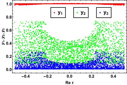
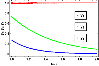
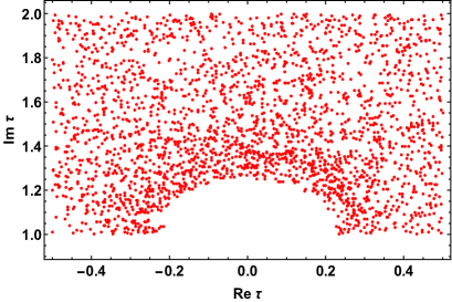
Figure 1: Top left and top right panel signify the correlation of the modular Yukawa couplings ($y_{1},y_{2},y_{3}$) with the real and imaginary parts of modulus $\tau$ respectively. The bottom panel represents the allowed region of the Re($\tau$) and Im($\tau$) abiding all the constraints and within the range of its fundamental domain.

Variation of the mixing angles with the sum of active neutrino masses, consistent with the allowed $3\sigma$ range are obtained, as shown in Fig. 2. In the left panel of Fig. 3, we show the correlation of Jarsklog CP invariant with the reactor mixing angle allowed by the neutrino oscillation data, which is found to be of the order of ${\cal O}(10^{-3})$. The right panel of Fig. 3, signifies the full parameter space for Yukawa couplings as per the observed sum of active neutrino masses. In Fig. 4, we have displayed a correlation of the Yukawa couplings $y_{1}$ with $y_{2}$ and $y_{2}$ with $y_{3}$ in the left and right panels respectively. The effective neutrinoless double beta decay mass parameter $|m_{ee}|$ for both normal and inverted orderings is found to have a maximum value of $55$ meV from the variation of observed sum of active neutrino masses, which is presented in the left panel of Fig. 5. The results for normal and inverted hierarchies are shown by the blue and red points. The horizontal pink and cyan bands represent the $3\sigma$ sensitivity limits of current GERDA and the future LEGEND-200 experiments respectively. It should be noted from the figure that the model predictions for $|m_{ee}|$ are within the reach of the future generation experiments and the inverted hierarchical region is more favoured. The right panel represents the correlation between heavy fermion masses $M_{2}$ and $M_{3}$.

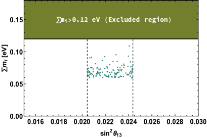
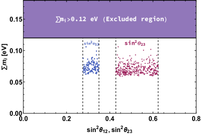
Figure 2: Left (Right) panel represents the correlation between $\sin^{2}\theta_{13}$ ($\sin^{2}\theta_{12}$ and $\sin^{2}\theta_{23}$) with the sum of active neutrino masses.

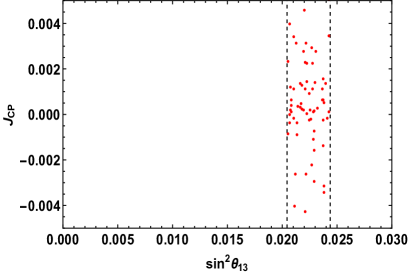
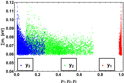
Figure 3: Left panel displays the correlation of Jarsklog invariant with the reactor mixing angle and right panel reflects the variation of modular Yukawa couplings with the sum of active neutrino masses.

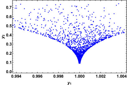
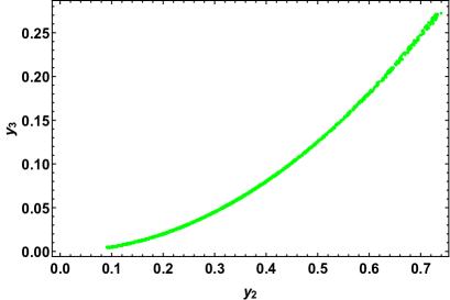
Figure 4: Left (Right) panel displays the correlation between $y_{1}$ and $y_{2}$ ($y_{2}$ and $y_{3}$).

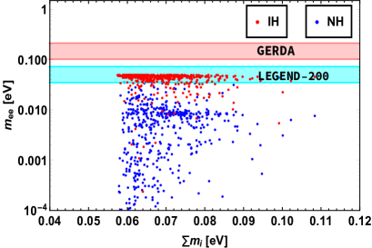
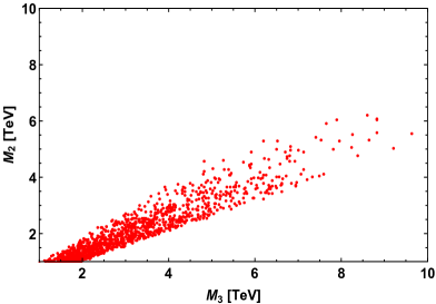
Figure 5: Left panel shows the correlation of effective neutrino mass of neutrinoless double beta decay with the sum of active neutrino masses, where the blue and red points correspond to normal and inverted hierarchies. The horizontal pink band corresponds to the $3\sigma$ sensitivity limit of currently running GERDA experiment and the cyan band represents the $3\sigma$ limit of the future LEGEND-200 experiment. Right panel depicts correlation between the heavy fermion masses $M_{2}$ and $M_{3}$.

Comment on non-unitarity

Here, we briefly comment on non-unitarity of neutrino mixing matrix $U^{\prime}_{\rm PMNS}$ in the presence of heavy fermionic superfields. The standard parametrization for the deviation from unitarity can be expressed as Forero:2011pc

$$U^{\prime}_{\rm PMNS}\equiv\left(1-\frac{1}{2}FF^{\dagger}\right)U_{\rm PMNS}.$$ (38)

Here, $U_{\rm PMNS}$ is the PMNS mixing matrix which diagonalises the mass matrix of the three light neutrinos and $F$ is the mixing of active neutrinos with the heavy fermions and approximated as $F\equiv(M^{T}_{RS})^{-1}M_{D}\approx\frac{\alpha_{D}v}{\alpha_{NS}v_{\rho}}$, which is a hermitian matrix. The global constraints on the non-unitarity parameters Antusch:2014woa ; Blennow:2016jkn ; Fernandez-Martinez:2016lgt , are found via several experimental results such as the $W$ boson mass $M_{W}$, the Weinberg angle $\theta_{W}$, several ratios of $Z$ boson fermionic decays as well as its invisible decay, electroweak universality, CKM unitarity bounds, and lepton flavor violations. In our model framework, we consider the following approximated normalized order for the Dirac, pseudo-Dirac and heavy fermion masses to correctly generate the observed mass-squared differences as well as the sum of active neutrino masses of desired order

$$\left(\frac{m_{\nu}}{0.1~{}{\rm eV}}\right)\approx\left(\frac{M_{D}}{10^{-3}~{}~{}{\rm GeV}}\right)\left(\frac{M_{RS}}{10^{3}~{}~{}{\rm GeV}}\right)^{-1}\left(\frac{M_{LS}}{10^{-4}~{}~{}{\rm GeV}}\right).$$ (39)

Therefore, with the chosen order of masses, we obtain an approximated non-unitary mixing for the present model as

$$|FF^{\dagger}|\leq\left[\begin{array}[]{ccc}6.06\times 10^{-13}&4.25\times 10^{-14}&6.9\times 10^{-14}\\ 4.25\times 10^{-14}&2.77\times 10^{-13}&1.14\times 10^{-12}\\ 6.9\times 10^{-14}&1.14\times 10^{-12}&7.25\times 10^{-13}\\ \end{array}\right].$$ (43)

Since, the mixing between the active and heavy fermions in our model is found to be very small, it leads to a negligible contribution to the non-unitarity.

Comment on lepton flavor violation

Here, we will briefly discuss about the prospect of lepton flavor violation (LFV) effect, in particular $\ell_{i}\to\ell_{j}\gamma$ decays, in the context of present model. Lepton flavor violating decays are strictly forbidden in the SM and are known to be induced in models with extended lepton sectors. The current limit on these branching ratios are: ${\rm Br}(\mu\to e\gamma)<4.2\times 10^{-13}$ from MEG Collaboration TheMEG:2016wtm , ${\rm Br}(\tau\to e\gamma)<3.3\times 10^{-8}$ and ${\rm Br}(\tau\to\mu\gamma)<4.4\times 10^{-8}$ from BABAR collaboration Aubert:2009ag .

In this model, the lepton flavor violating decays ($\ell_{i}\to\ell_{j}\gamma$) can occur via exchange of heavy fermions at one loop level Bernabeu:1987gr ; Deppisch:2004fa , as there is mixing between the light and heavy fermions and the corresponding dominant one-loop contribution to the branching ratios for these decays is given as Ilakovac:1994kj ; Forero:2011pc

$$\text{Br}(\ell_{i}\to\ell_{j}\gamma)=\frac{\alpha_{W}^{3}s_{W}^{2}}{256\pi^{2}}\frac{m_{\ell_{i}}^{5}}{M_{W}^{4}}\frac{1}{\Gamma_{\ell_{i}}}|G_{ij}^{W}|^{2},$$ (44)

where $G_{ij}^{W}$ is loop functions whose analytic form is

$$G_{ij}^{W} = \sum_{k=1}^{3}F_{ik}F_{jk}^{\dagger}G_{\gamma}^{W}\left(\frac{\ M_{N_{k}}^{2}}{M_{W}^{2}}\right)~{}~{}~{}~{}~{}\text{with}$$

$$G_{\gamma}^{W}(x) = \frac{1}{12(1-x)^{4}}(10-43x+78x^{2}-49x^{3}+4x^{4})\;.$$ (45)

Here, $M_{N_{k}}$ represents heavy neutrino superfields and $F$ characterises the mixing of active neutrinos with the heavy fermions leading to non-unitarity effect. Since in the present model, the non-unitarity parameters are found to be extremely small (43), the branching ratios of the LFV decays are highly suppressed. Thus, for TeV scale heavy fermions $M_{N_{k}}$, the branching ratios for different LFV decays are found to be

$${\rm Br}(\mu\to e\gamma)\leq 8.9\times 10^{-33}\left(\frac{|(FF^{\dagger})_{\mu e}|}{4.25\times 10^{-14}}\right)^{2},$$

$${\rm Br}(\tau\to e\gamma)\leq 4.2\times 10^{-33}\left(\frac{|(FF^{\dagger})_{\tau e}|}{6.9\times 10^{-14}}\right)^{2},$$

$${\rm Br}(\tau\to\mu\gamma)\leq 1.2\times 10^{-30}\left(\frac{|(FF^{\dagger})_{\tau\mu}|}{1.14\times 10^{-12}}\right)^{2},$$ (46)

which are beyond the reach of any of the future experiments.

IV Leptogenesis

Leptogenesis has proven to be one of the most preferred way to generate the observed baryon asymmetry of the Universe. The standard scenario of resonant enhancement in CP asymmetry has brought down the scale as low as TeV Pilaftsis:1997jf ; Bambhaniya:2016rbb ; Pilaftsis:2003gt ; Abada:2018oly . The present model includes six heavy states with doubly degenerate masses for each pair Eqn. (27). But one can introduce a higher dimensional mass term for the heavy neutrino superfield ($S_{L}^{c}$) as

$$L_{M}=-\alpha_{R}Y{S^{c}_{L}}S^{c}_{L}\frac{\rho^{4}}{\Lambda^{3}}.$$ (47)

This leads to a small mass splitting between the heavy superfields, there by enhancing the CP asymmetry to generate required lepton asymmetry Pilaftsis:2005rv ; Asaka:2018hyk . Thus, one can construct the right-handed Majorana mass matrix as follows

$$M_{R}=\frac{\alpha_{R}v^{4}_{\rho}}{6\Lambda^{3}}\begin{pmatrix}2y_{1}&-y_{3}&-y_{2}\\ -y_{3}&2y_{2}&-y_{1}\\ -y_{2}&-y_{1}&2y_{3}\end{pmatrix}.$$ (48)

The coupling $\alpha_{R}$ is chosen to be extremely small to retain the linear seesaw structure of the mass matrix Eqn. (32), i.e., $M_{D},M_{LS}\gg M_{R}$ and such inclusion does not affect the previous results. However, this term introduces a small mass splitting and the $2\times 2$ submatrix of Eqn. (32) in the $(N_{R},S^{c}_{L})$ basis, now can be written as

$$M=\begin{pmatrix}0&M_{RS}\\ M_{RS}^{T}&M_{R}\end{pmatrix}.$$ (49)

This matrix can have a block diagonal structure in the limit $\beta_{NS}\ll\alpha_{NS}$ by the unitary matrix $\frac{1}{\sqrt{2}}\begin{pmatrix}I&-I\\ I&I\end{pmatrix}$ as

$$M^{\prime}=\begin{pmatrix}M_{RS}+\frac{M_{R}}{2}&-\frac{M_{R}}{2}\\ -\frac{M_{R}}{2}&-M_{RS}+\frac{M_{R}}{2}\end{pmatrix}\approx\begin{pmatrix}M_{RS}+\frac{M_{R}}{2}&0\\ 0&-M_{RS}+\frac{M_{R}}{2}\end{pmatrix}.$$ (50)

Therefore, the mass eigenstates ($N^{\pm}$) are related to $N_{R}$ and $S^{c}_{L}$ through

$$\begin{pmatrix}S^{c}_{Li}\\ N_{Ri}\end{pmatrix}=\begin{pmatrix}\cos{\theta}&-\sin{\theta}\\ \sin{\theta}&\cos{\theta}\end{pmatrix}\begin{pmatrix}N_{i}^{+}\\ N_{i}^{-}\end{pmatrix}.$$ (51)

Assuming a maximal mixing, we can have

$$N_{Ri}=\frac{(N_{i}^{+}+N_{i}^{-})}{\sqrt{2}},~{}~{}S^{c}_{Li}=\frac{(N_{i}^{+}-N_{i}^{-})}{\sqrt{2}},$$ (52)

Thus, the interaction Lagrangian in Eqn.(3) can be written in the new basis $N_{i}^{\pm}$ as

$${\cal W}_{D} =\alpha_{D}{L}_{e_{L}}{H_{u}}\left[\bm{Y}\left(\frac{(N_{i}^{+}+N_{i}^{-})}{\sqrt{2}}\right)\right]_{1}+\beta_{D}{L}_{\mu_{L}}{H_{u}}\left[\bm{Y}\left(\frac{(N_{i}^{+}+N_{i}^{-})}{\sqrt{2}}\right)\right]_{1^{\prime}}$$ (53)

$$+\gamma_{D}{L}_{\tau_{L}}{H_{u}}\left[\bm{Y}\left(\frac{(N_{i}^{+}+N_{i}^{-})}{\sqrt{2}}\right)\right]_{1^{\prime\prime}}.$$

Analogously, the pseudo-Dirac interaction term Eqn. (11) becomes

$${\cal W}_{LS} =\alpha^{\prime}_{D}{L}_{e_{L}}{H_{u}}\left[\bm{Y}\left(\frac{(N_{i}^{+}-N_{i}^{-})}{\sqrt{2}}\right)\right]_{1}\frac{\rho^{3}}{\Lambda^{3}}+\beta^{\prime}_{D}{L}_{\mu_{L}}{H_{u}}\left[\bm{Y}\left(\frac{(N_{i}^{+}-N_{i}^{-})}{\sqrt{2}}\right)\right]_{1^{\prime}}\frac{\rho^{3}}{\Lambda^{3}}$$ (54)

$$+\gamma^{\prime}_{D}{L}_{\tau_{L}}{H_{u}}\left[\bm{Y}\left(\frac{(N_{i}^{+}-N_{i}^{-})}{\sqrt{2}}\right)\right]_{1^{\prime\prime}}\frac{\rho^{3}}{\Lambda^{3}}.$$

The mass eigenvalues for the new states $N^{+}$ and $N^{-}$ can be obtained by diagonalizing the block diagonal form of heavy superfield masses, expressed as

$$M_{RS}\pm\frac{M_{R}}{2}=\left(\frac{\alpha_{NS}v_{\rho}}{\sqrt{2}}\pm\frac{\alpha_{R}v^{4}_{\rho}}{4\Lambda^{3}}\right)\begin{pmatrix}2y_{1}&-y_{3}&-y_{2}\\ -y_{3}&2y_{2}&-y_{1}\\ -y_{2}&-y_{1}&2y_{3}\\ \end{pmatrix}.$$ (55)

In the above, the anti-symmetric part in $M_{RS}$ is neglected because $\beta_{NS}$ is small compared with $\alpha_{NS}$. The above matrix can be diagonalised through $(M^{\pm})_{\rm diag}=U_{\rm TBM}U_{R}\left(M_{RS}\pm\frac{M_{R}}{2}\right)U^{T}_{R}U^{T}_{\rm TBM}$, with mass eigenvalues

$$M^{\pm}_{1}\approx\frac{1}{6}\left(\frac{\alpha_{NS}v_{\rho}}{\sqrt{2}}\pm\frac{\alpha_{R}v^{4}_{\rho}}{4\Lambda^{3}}\right)\left(y_{1}+2y_{2}-\sqrt{9y^{2}_{1}+12y_{1}y_{2}+12y^{2}_{2}}\right),$$

$$M^{\pm}_{2}\approx\frac{1}{6}\left(\frac{\alpha_{NS}v_{\rho}}{\sqrt{2}}\pm\frac{\alpha_{R}v^{4}_{\rho}}{4\Lambda^{3}}\right)\left(y_{1}+2y_{2}+\sqrt{9y^{2}_{1}+12y_{1}y_{2}+12y^{2}_{2}}\right),$$

$$M^{\pm}_{3}\approx\frac{1}{3}\left(\frac{\alpha_{NS}v_{\rho}}{\sqrt{2}}\pm\frac{\alpha_{R}v^{4}_{\rho}}{4\Lambda^{3}}\right)\left(y_{1}+2y_{2}\right).$$ (56)

Here, $U_{\rm TBM}$ is the tribimaximal mixing matrix Harrison:2002er ; Harrison:2002kp and

$$U_{R}\approx\begin{pmatrix}B_{-}&\frac{1}{\sqrt{X_{-}}}&0\\ 0&0&1\\ B_{+}&\frac{1}{\sqrt{X_{+}}}&0\end{pmatrix},$$ (57)

with

$$B_{\pm}=-\frac{y_{1}+2y_{2}\pm\sqrt{9y^{2}_{1}-12y_{1}y_{2}+12y^{2}_{2}}}{2\sqrt{2}(y_{1}-y_{2})},~{}~{}{\rm and}~{}~{}X_{\pm}=\sqrt{1+B^{2}_{\pm}}\;.$$ (58)

As noticed from Eqn. (56), we get three sets of nearly degenerate mass states after diagonalization. We further assume that the lightest pair with TeV scale masses dominantly contribute to the CP asymmetry. The small mass splitting between the lightest states implies the contribution from one loop self energy of heavy particle decay dominates over the vertex diagram. The expression for CP asymmetry is given by Pilaftsis:1997jf ; Gu:2010xc

$$\epsilon_{N^{-}_{i}}\approx\frac{1}{32\pi^{2}A_{N^{-}_{i}}}{\rm Im}\left[\left(\frac{\tilde{M_{D}}}{v_{u}}-\frac{\tilde{M}_{LS}}{v_{u}}\right)^{\dagger}\left(\frac{\tilde{M}_{D}}{v_{u}}+\frac{\tilde{M}_{LS}}{v_{u}}\right)^{2}\left(\frac{\tilde{M}_{D}}{v_{u}}-\frac{\tilde{M}_{LS}}{v_{u}}\right)^{\dagger}\right]_{ii}\frac{r_{N}}{r^{2}_{N}+4A^{2}_{N^{-}_{i}}}.$$

Here, $\tilde{M}_{D}=M_{D}U_{\rm TBM}U_{R}$, $\tilde{M}_{LS}=M_{LS}U_{\rm TBM}U_{R}$ and $\Delta M=M^{+}_{i}-M^{-}_{i}\approx M_{R}$. The parameters $r_{N}$ and $A_{N^{-}}$ are expressed as

$$r_{N}=\frac{{(M^{+}_{i})}^{2}-{(M^{-}_{i})}^{2}}{M^{+}_{i}M^{-}_{i}}=\frac{\Delta M(M^{+}_{i}+M^{-}_{i})}{M^{+}_{i}M^{-}_{i}}\;,$$

$$A_{N^{-}}\approx\frac{1}{16\pi}\left[\left(\frac{\tilde{M}_{D}}{v_{u}}-\frac{\tilde{M}_{LS}}{v_{u}}\right)\left(\frac{\tilde{M}_{D}}{v_{u}}+\frac{\tilde{M}_{LS}}{v_{u}}\right)\right]_{ii}.$$ (60)

It should be noted that because of the imposition of modular symmetry, which plays the role of eliminating the usage of extra flavon fields, the CP asymmetry parameter crucially depends on the Yukawa couplings $\bf Y$ = $(y_{1},y_{2},y_{3})$, apart from other free parameters of the model and the flavon VEV $v_{\rho}$. However, essentially there is no freedom in the choice of how much can be the numerical values of the Yukawa couplings as they depend on the real and imaginary part of the modulus $\tau$, which are constrained by the neutrino oscillation data. In the left (middle) panel of Fig. 6, we show the variation of CP asymmetry with the magnitude (argument) of the Yukawa coupling $y_{1}$ and right panel projects its behavior with $r_{N}$. It should be noted that, the CP symmetry in the context of the present model is broken by the vacuum expectation value of the modulus $\tau$. As this vacuum expectation value is related to the CP phases in the PMNS matrix and the CP asymmetry of leptogenesis, it is generally anticipated that there should be a non-trivial correlation between these observables. In the bottom panel of Fig. 6, we show the correlation plot between the Dirac CP violating phase $\delta_{CP}$ and the CP asymmetry of leptogenesis, which depicts no appreciable correlation between these observables.

In Table. 3, we provide benchmark values that satisfy both neutrino mass and required CP asymmetry for leptogenesis Davidson:2008bu ; Buchmuller:2004nz (to be discussed in the next subsection).

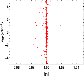
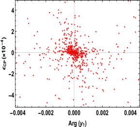
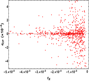
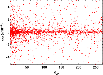
Figure 6: Left and middle panels represent the variation of CP asymmetry with the magnitude and argument of Yukawa coupling respectively. Right panel shows its dependence with parameter $r_{N}$. Whereas, the bottom plot represents the correlation between CP asymmetry and the CP violating phase $\delta_{CP}$.

$\epsilon^{e}_{N^{-}}$	$\epsilon^{\mu}_{N^{-}}$	$\epsilon^{\tau}_{N^{-}}$	$\epsilon_{N^{-}}$	$\Delta M$ (GeV)
$-9\times 10^{-5}$	$-2.13\times 10^{-4}$	$-2.42\times 10^{-4}$	$-5.45\times 10^{-4}$	$2.94\times 10^{-5}$

Table 3: CP asymmetries and mass splitting obtained from the allowed range of model parameters which satisfy neutrino oscillation data.

IV.1 One flavor approximation

The evolution of lepton asymmetry can be deduced from the dynamics of relevant Boltzmann equations. Sakharov criteria Sakharov:1967dj demand the decay of parent fermion to be out of equilibrium to generate the lepton asymmetry. To impose this condition, one has to compare the Hubble rate with the decay rate as follows.

$$K=\frac{\Gamma_{N^{-}_{1}}}{H(T=M^{-}_{1})}\;.$$ (61)

Here, $H=\frac{1.67\sqrt{g_{\star}}~{}T^{2}}{M_{\rm Pl}}$, with $g_{\star}=106.75$, $M_{\rm Pl}=1.22\times 10^{19}$ GeV. We consider the coupling strength $\left(\approx\left(\frac{\sqrt{2}M_{D}}{v}U_{\rm TBM}U_{R}\right)_{ij}\right)$ roughly around $10^{-6}$, where the minimum order of coupling parameters are taken from the numerical analysis section, consistent with neutrino oscillation data. The Boltzmann equations for the evolution of the number densities of right-handed superfield and lepton, written in terms of yield parameter (ratio of number density to entropy density) are given by Plumacher:1996kc ; Giudice:2003jh ; Buchmuller:2004nz ; Strumia:2006qk ; Iso:2010mv

$$\frac{dY_{N^{-}}}{dz}=-\frac{z}{sH(M_{1}^{-})}\left[\left(\frac{Y_{N^{-}}}{{Y^{\rm eq}_{N^{-}}}}-1\right)\gamma_{D}+\left(\left(\frac{{Y_{N^{-}}}}{{Y^{\rm eq}_{N^{-}}}}\right)^{2}-1\right)\gamma_{S}\right],$$

$$\frac{dY_{B-L}}{dz}=-\frac{z}{sH(M_{1}^{-})}\left[\epsilon_{N^{-}}\left(\frac{Y_{N^{-}}}{{Y^{\rm eq}_{N^{-}}}}-1\right)\gamma_{D}-\frac{Y_{B-L}}{{Y^{\rm eq}_{\ell}}}\frac{\gamma_{D}}{2}\right],$$ (62)

where $s$ denotes the entropy density, $z=M^{-}_{1}/T$ and the equilibrium number densities are given by Davidson:2008bu

$$Y^{\rm eq}_{N^{-}}=\frac{45g_{N^{-}}}{4{\pi}^{4}g_{\star}}z^{2}K_{2}(z),\hskip 8.53581pt{Y^{\rm eq}_{\ell}}=\frac{3}{4}\frac{45\zeta(3)g_{\ell}}{2{\pi}^{4}g_{\star}}\,.$$ (63)

Here, $K_{1,2}$ denote modified Bessel functions, $g_{\ell}=2$ and $g_{N^{-}}=2$ denote the degrees of freedom of lepton and right-handed superfields respectively. The decay rate $\gamma_{D}$ is given by

$$\gamma_{D}=sY^{\rm eq}_{N^{-}}\Gamma_{D},$$ (64)

where, $\Gamma_{D}=\Gamma_{N^{-}}\frac{K_{1}(z)}{K_{2}(z)}$. $\gamma_{S}$ denotes the scattering rate of the decaying particle i.e.,$N_{1}^{-}N_{1}^{-}\to\rho\rho$ Iso:2010mv . The Boltzmann equation for $Y_{B-L}$ is free from the subtlety of asymmetry getting produced even when $N_{1}^{-}$ is in thermal equilibrium i.e., by subtracting the on-shell $N_{1}^{-}$ exchange contribution ($\frac{\gamma_{D}}{4}$) from the $\Delta L=2$ process Giudice:2003jh .

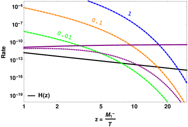
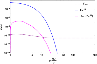
Figure 7: Left panel projects the comparison of interaction rates with Hubble expansion, where purple lines correspond to decay (solid), inverse decay (dotted) and scattering rates plotted for various values of Majorana coupling (green, orange, blue). Right panel projects the evolution of $Y_{B-L}$ (dashed) as a function of $z=M_{1}^{-}/{T}$.

The interaction rates are compared with Hubble expansion in the left panel of Fig. 7. The decay ($\Gamma_{D}$) and inverse decay $\left(\Gamma_{D}\frac{Y^{\rm eq}_{N^{-}}}{Y^{\rm eq}_{\ell}}\right)$ rates are plotted in purple with the coupling strength $\sim 10^{-6}$. The scattering rate $\left(\frac{\gamma_{S}}{sY^{\rm eq}_{N^{-}}}\right)$ for $N_{1}^{-}N_{1}^{-}\to\rho\rho$ is projected for various set of values for coupling (of Eq. LABEL:Eq:yuk-M), consistent with neutrino oscillation study. For larger Majorana coupling, the scattering process makes $N_{1}^{-}$ to stay longer in thermal soup and hence, number density of $N_{1}^{-}$ depletes in annihilation rather than decay, generating lesser lepton asymmetry. In one-flavor approximation, the solution of Boltzmann eqns (62) using the benchmark given in Table. 3 is projected in the right panel of Fig. 7 with the inclusion of decay and scattering rates. Once the out-of-equilibrium criteria is satisfied, the decay proceeds slow (over abundance), $Y_{N^{-}}$ does not trace $Y^{\rm eq}_{N^{-}}$ (magenta curve) and the lepton asymmetry (dashed curve) is generated. The obtained lepton asymmetry gets converted to the observed baryon asymmetry through sphaleron transition, given by Harvey:1990qw

$$Y_{B}=\left(\frac{8N_{f}+4N_{H}}{22N_{f}+13N_{H}}\right)Y_{B-L}.$$ (65)

Here, $N_{f}$ denotes the number of superfields generations and $N_{H}$ is the number of Higgs doublets. The observed baryon asymmetry is quantified in terms of baryon to photon ratio Aghanim:2018eyx

$$\eta=\frac{\eta_{b}-\eta_{\bar{b}}}{\eta_{\gamma}}=6.08\times 10^{-10}.$$ (66)

Based on the relation $Y_{B}=(7.04)^{-1}\eta$, the current bound on baryon asymmetry is $Y_{B}\sim 0.86\times 10^{-10}$.

We observe the same Yukawas i.e. Y=($y_{1},y_{2},y_{3}$) are involved in both Dirac as well as Majorana masses and hence, appear not only in the neutrino phenomenology but also in computation related to leptogenesis. But the values of these couplings are strongly constrained from the real and imaginary part of the complex modulus $\tau$. Thus, the free parameters play an important role in adjusting the parameter space to generate a successful leptogenesis.

IV.2 Flavor consideration

One flavor approximation is probable at high scale ($T>10^{12}$ GeV), where all the Yukawa interactions are out of equilibrium. But for temperatures below $10^{12}$ GeV, various charged lepton Yukawa couplings come into equilibrium and hence flavor effects play a crucial role in generating the final lepton asymmetry. For temperatures below $10^{5}$ GeV, all the Yukawa interactions are in equilibrium and the asymmetry is stored in the individual lepton sector. The detailed investigation of flavor effects in type-I leptogenesis can be found in the literature Pascoli:2006ci ; Antusch:2006cw ; Nardi:2006fx ; Abada:2006ea ; Granelli:2020ysj ; Dev:2017trv .

The Boltzmann equation for generating the lepton asymmetry in each flavor is Antusch:2006cw

$$\frac{dY^{\alpha}_{B-L_{\alpha}}}{dz}=-\frac{z}{sH(M_{1}^{-})}\left[\epsilon^{\alpha}_{N^{-}}\left(\frac{Y_{N^{-}}}{{Y^{eq}_{N^{-}}}}-1\right)\gamma_{D}-\left(\frac{\gamma^{\alpha}_{D}}{2}\right)\frac{A_{\alpha\alpha}Y^{\alpha}_{\rm B-L_{\alpha}}}{{Y^{eq}_{\ell}}}\right],$$ (67)

where, $\epsilon^{\alpha}_{N^{-}}$ represents the CP asymmetry in each lepton flavor and

$$\gamma_{D}^{\alpha}=sY_{N^{-}}^{eq}\Gamma_{N^{-}}^{\alpha}\frac{K_{1}(z)}{K_{2}(z)},\quad\gamma_{D}=\sum_{\alpha}\gamma^{\alpha}_{D},\\$$

The matrix $A$ is given by Nardi:2006fx ,

$$A=\begin{pmatrix}-\frac{221}{711}&&\frac{16}{711}&&\frac{16}{711}\\ \frac{16}{711}&&-\frac{221}{711}&&\frac{16}{711}\\ \frac{16}{711}&&\frac{16}{711}&&-\frac{221}{711}\\ \end{pmatrix}.\\$$

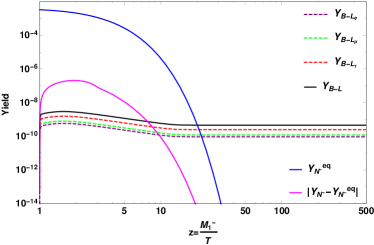
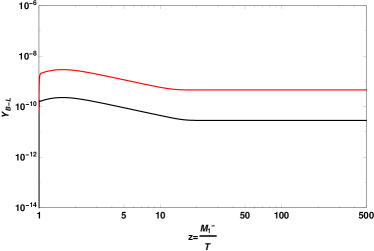
Figure 8: The left panel displays yield with inclusion of flavor effects. The right panel shows the enhancement in the yield due to three-flavor calculation (red curve) over one-flavor approximation (black curve).

From the benchmark shown in Table. 3, we project the $B-L$ yield with flavor consideration in the left panel of Fig. 8. It is clear that a notable enhancement in $B-L$ asymmetry is obtained in case of flavor consideration (red curve) over one flavor approximation (black curve), as displayed in the right panel. This is because, in one flavor approximation the decay of heavy fermion to a specific lepton flavor final state can get washed out by the inverse decays of any flavor unlike the flavored case Abada:2006ea .

V Comment on collider studies

Here, we briefly comment on the most promising collider signature of heavy pseudo-Dirac neutrinos without going into any detailed estimation, in the context of the present model. In the linear seesaw scenario the $M_{LS}$ is the lepton number violating term han2021full therefore its mass scale is naturally small. Also the effective Majorana neutrino mass matrix as shown in eqn.(33) for active neutrino where the smallness of $m_{\nu}$ is attributed due to $M_{LS}$ being the pseudo-Dirac neutrino mass term and further suppressed by the ratio of $M_{D}$ and $M_{RS}$. Hence, the seesaw scale can be lowered to TeV range which is experimentally accessible at LHC. The trilepton plus missing energy process as mentioned in eqn.(68), which can be studied at colliders, is an interesting mechanism involving heavy pseudo-Dirac neutrinos Das:2014jxa :

$$\sigma(pp\to\ell^{\pm}\ell^{\pm}\ell^{\mp}+\not{E}_{T})\ =\sigma(pp\to W^{*\pm}\to N\ell^{\pm})\times\mathrm{Br}(N\to\ell^{\mp}W^{\pm})\times\mathrm{Br}(W^{\pm}\to\ell^{\pm}+\nu(\bar{\nu})),$$ (68)

where it is assumed that the heavy neutrinos are heavier than the $W$ boson, so that the two-body decay process $N\to\ell W$ is kinematically allowed, followed by the on-shell $W$ decaying into SM leptons. Its viability is essentially determined by firstly, large mixing between active-sterile neutrinos i.e. $\mathsf{\Theta}_{\nu RS}\simeq\sqrt{\nicefrac{{m_{\nu}}}{{M_{RS}}}}\leq 10^{-6}$ Aguilar-Saavedra:2009fxa , secondly, masses of heavy pseudo-Dirac neutrinos ranging from few [GeV-TeV], and finally its production mechanism.

VI Conclusion

We have investigated a modular form of $A_{4}$ flavor symmetry that reduces the complications of accommodating multiple flavons. The present model includes three right-handed and three left-handed heavy superfields to explore the neutrino phenomenology within the framework of linear seesaw in SUSY context. We have considered the Yukawa couplings to transform non-trivially under modular $A_{4}$ group, which replaces the role of conventional flavon fields. This leads to a specific flavor structure of the neutrino mass matrix and helps in studying the neutrino mixing. We numerically diagonalized the neutrino mass matrix to obtain an allowed region for the model parameters compatible with the current $3\sigma$ limit of oscillation data. The flavor structure of heavy superfields gives rise to six doubly degenerate mass eigenstates and hence, to explain leptogenesis, we introduced a higher dimensional mass term for the right-handed superfields to generate a small mass splitting. We obtained a non-zero CP asymmetry from the decay of lightest heavy fermion eigen state and the self energy contribution is partially enhanced due to the small mass difference between the two lighter heavy fermion superfields. Using a specific benchmark of model parameters consistent with oscillation data, we solved coupled Boltzmann equations to obtain the evolution of lepton asymmetry at TeV scale which comes out to be of the order $\approx 10^{-10}$, which is sufficient to explain the present baryon asymmetry of the Universe. Furthermore, we have also discussed the enhancement in asymmetry with flavor consideration. The promising collider signature of the heavy pseudo-Dirac neutrinos is the trilepton plus missing energy, which depend crucially on the mixing between the light active and pseudo-Dirac neutrinos, mass of these heavy neutrinos and their production mechanism.

Appendix

$\bar{\Gamma}$ is the modular group which attains a linear fractional transformation $\gamma$ which acts on modulus $\tau$ linked to the upper-half complex plane whose transformation is given by

$$\tau\longrightarrow\gamma\tau=\frac{a\tau+b}{c\tau+d}\ ,~{}~{}{\rm where}~{}~{}a,b,c,d\in\mathbb{Z}~{}~{}{\rm and}~{}~{}ad-bc=1,~{}~{}{\rm Im}[\tau]>0~{},$$ (69)

where it is isomorphic to the transformation$PSL(2,\mathbb{Z})=SL(2,\mathbb{Z})/\{I,-I\}$. The $S$ and $T$ transformation helps in generating the modular transformation defined by

$$S:\tau\longrightarrow-\frac{1}{\tau}\ ,\qquad\qquad T:\tau\longrightarrow\tau+1\ ,$$ (70)

and hence the algebric relations so satisfied are as follows,

$$S^{2}=\mathbb{I}\ ,\qquad(ST)^{3}=\mathbb{I}\ .$$ (71)

Here, series of groups are introduced, $\Gamma(N)~{}(N=1,2,3,\dots)$ and defined as

$$\begin{aligned} \Gamma(N)=\left\{\begin{pmatrix}a&b\\ c&d\end{pmatrix}\in SL(2,\mathbb{Z})~{},~{}~{}\begin{pmatrix}a&b\\ c&d\end{pmatrix}=\begin{pmatrix}1&0\\ 0&1\end{pmatrix}~{}~{}({\rm mod}N)\right\}\end{aligned}.$$ (72)

Definition of $\bar{\Gamma}(2)\equiv\Gamma(2)/\{I,-I\}$ for $N=2$. Since $-I$ is not associated with $\Gamma(N)$ for $N>2$ case, one can have $\bar{\Gamma}(N)=\Gamma(N)$, which are infinite normal subgroup of $\bar{\Gamma}$ known as principal congruence subgroups. Quotient groups come from the finite modular group defined as $\Gamma_{N}\equiv\bar{\Gamma}/\bar{\Gamma}(N)$. Imposition of $T^{N}=\mathbb{I}$, is done for these finite groups $\Gamma_{N}$. Thus, the groups $\Gamma_{N}$ ($N=2,3,4,5$) are isomorphic to $S_{3}$, $A_{4}$, $S_{4}$ and $A_{5}$, respectively deAdelhartToorop:2011re . $N$ level modular forms are holomorphic functions $f(\tau)$ which are transformed under the influence of $\Gamma(N)$ as follows:

$$f(\gamma\tau)=(c\tau+d)^{k}f(\tau)~{},~{}~{}\gamma\in\Gamma(N)~{},$$ (73)

where $k$ is the modular weight.

Here the discussion is all about the modular symmetric theory. This paper comprises of $A_{4}$ ($N=3$) modular group. A field $\phi^{(I)}$ transforms under the modular transformation of Eq.(69), as

$$\phi^{(I)}\to(c\tau+d)^{-k_{I}}\rho^{(I)}(\gamma)\phi^{(I)},$$ (74)

where $-k_{I}$ represents the modular weight and $\rho^{(I)}(\gamma)$ signifies an unitary representation matrix of $\gamma\in\Gamma(2)$.

The scalar fields^′ kinetic term is as follows

$$\sum_{I}\frac{|\partial_{\mu}\phi^{(I)}|^{2}}{(-i\tau+i\bar{\tau})^{k_{I}}}~{},$$ (75)

which doesn’t change under the modular transformation and eventually the overall factor is absorbed by the field redefinition. Thus, the Lagrangian should be invariant under the modular symmetry.

The modular forms of the Yukawa coupling Y = $(y_{1},y_{2},y_{3})$ with weight 2, which transforms as a triplet of $A_{4}$ can be expressed in terms of Dedekind eta-function $\eta(\tau)$ and its derivative Feruglio:2017spp :

$$y_{1}(\tau) = \frac{i}{2\pi}\left(\frac{\eta^{\prime}(\tau/3)}{\eta(\tau/3)}+\frac{\eta^{\prime}((\tau+1)/3)}{\eta((\tau+1)/3)}+\frac{\eta^{\prime}((\tau+2)/3)}{\eta((\tau+2)/3)}-\frac{27\eta^{\prime}(3\tau)}{\eta(3\tau)}\right),$$

$$y_{2}(\tau) = \frac{-i}{\pi}\left(\frac{\eta^{\prime}(\tau/3)}{\eta(\tau/3)}+\omega^{2}\frac{\eta^{\prime}((\tau+1)/3)}{\eta((\tau+1)/3)}+\omega\frac{\eta^{\prime}((\tau+2)/3)}{\eta((\tau+2)/3)}\right),$$ (76)

$$y_{3}(\tau) = \frac{-i}{\pi}\left(\frac{\eta^{\prime}(\tau/3)}{\eta(\tau/3)}+\omega\frac{\eta^{\prime}((\tau+1)/3)}{\eta((\tau+1)/3)}+\omega^{2}\frac{\eta^{\prime}((\tau+2)/3)}{\eta((\tau+2)/3)}\right)\,.$$

It is interesting to note that the couplings those are defined as singlet under $A_{4}$ start from $-k=4$ while they are zero if $-k=2$.

References

- (1) A. Faessler, Status of the determination of the electron–neutrino mass, Prog. Part. Nucl. Phys. 113 (2020) 103789.
- (2) KATRIN collaboration, M. Aker et al., Improved Upper Limit on the Neutrino Mass from a Direct Kinematic Method by KATRIN, Phys. Rev. Lett. 123 (2019) 221802 [arXiv:1909.06048].
- (3) B. Pontecorvo, Neutrino Experiments and the Problem of Conservation of Leptonic Charge, Sov. Phys. JETP 26 (1968) 984.
- (4) F. Feruglio, Neutrino masses and mixing angles: A tribute to Guido Altarelli, Frascati Phys. Ser. 64 (2017) 174.
- (5) Particle Data Group collaboration, M. Tanabashi et al., Review of Particle Physics, Phys. Rev. D98 (2018) 030001.
- (6) S. Weinberg, Varieties of Baryon and Lepton Nonconservation, Phys. Rev. D22 (1980) 1694.
- (7) S. Weinberg, Baryon and Lepton Nonconserving Processes, Phys. Rev. Lett. 43 (1979) 1566.
- (8) F. Wilczek and A. Zee, Operator Analysis of Nucleon Decay, Phys. Rev. Lett. 43 (1979) 1571.
- (9) P. Minkowski, at a Rate of One Out of Muon Decays?, Phys. Lett. 67B (1977) 421.
- (10) R.N. Mohapatra and G. Senjanovic, Neutrino Mass and Spontaneous Parity Nonconservation, Phys. Rev. Lett. 44 (1980) 912.
- (11) M. Gell-Mann, P. Ramond and R. Slansky, Complex Spinors and Unified Theories, Conf. Proc. C790927 (1979) 315 [arXiv:1306.4669].
- (12) A. Zee, A Theory of Lepton Number Violation, Neutrino Majorana Mass, and Oscillation, Phys. Lett. 93B (1980) 389.
- (13) K.S. Babu, Model of ’Calculable’ Majorana Neutrino Masses, Phys. Lett. B203 (1988) 132.
- (14) N. Arkani-Hamed, S. Dimopoulos, G.R. Dvali and J. March-Russell, Neutrino masses from large extra dimensions, Phys. Rev. D65 (2001) 024032 [hep-ph/9811448].
- (15) R.N. Mohapatra and J.W.F. Valle, Neutrino Mass and Baryon Number Nonconservation in Superstring Models, Phys. Rev. D34 (1986) 1642.
- (16) M.C. Gonzalez-Garcia and J.W.F. Valle, Fast Decaying Neutrinos and Observable Flavor Violation in a New Class of Majoron Models, Phys. Lett. B216 (1989) 360.
- (17) A. Cárcamo Hernández, J. Marchant González and U. Saldaña-Salazar, Viable low-scale model with universal and inverse seesaw mechanisms, Phys. Rev. D 100 (2019) 035024 [arXiv:1904.09993].
- (18) M. Malinsky, J.C. Romao and J.W.F. Valle, Novel supersymmetric SO(10) seesaw mechanism, Phys. Rev. Lett. 95 (2005) 161801 [hep-ph/0506296].
- (19) R.N. Mohapatra et al., Theory of neutrinos: A White paper, Rept. Prog. Phys. 70 (2007) 1757 [hep-ph/0510213].
- (20) E. Ma and G. Rajasekaran, Softly broken A(4) symmetry for nearly degenerate neutrino masses, Phys. Rev. D 64 (2001) 113012 [hep-ph/0106291].
- (21) S. Pakvasa and H. Sugawara, Discrete Symmetry and Cabibbo Angle, Phys. Lett. B 73 (1978) 61.
- (22) F. Feruglio, Are neutrino masses modular forms?, p. 227. 2019. arXiv:1706.08749. 10.1142/9789813238053_0012.
- (23) S.J. King and S.F. King, Fermion Mass Hierarchies from Modular Symmetry, arXiv:2002.00969.
- (24) S. King, Unified Models of Neutrinos, Flavour and CP Violation, Prog. Part. Nucl. Phys. 94 (2017) 217 [arXiv:1701.04413].
- (25) G. Altarelli and F. Feruglio, Discrete Flavor Symmetries and Models of Neutrino Mixing, Rev. Mod. Phys. 82 (2010) 2701 [arXiv:1002.0211].
- (26) H. Ishimori, T. Kobayashi, H. Ohki, Y. Shimizu, H. Okada and M. Tanimoto, Non-Abelian Discrete Symmetries in Particle Physics, Prog. Theor. Phys. Suppl. 183 (2010) 1 [arXiv:1003.3552].
- (27) S.F. King, Models of Neutrino Mass, Mixing and CP Violation, J. Phys. G 42 (2015) 123001 [arXiv:1510.02091].
- (28) M. Abbas, Flavor masses and mixing in modular 4 Symmetry, arXiv:2002.01929.
- (29) X. Wang, Lepton Flavor Mixing and CP Violation in the Minimal Type-(I+II) Seesaw Model with a Modular Symmetry, arXiv:1912.13284.
- (30) J.N. Lu, X.G. Liu and G.J. Ding, Modular symmetry origin of texture zeros and quark lepton unification, Phys. Rev. D 101 (2020) 115020 [arXiv:1912.07573].
- (31) T. Kobayashi, T. Nomura and T. Shimomura, Type II seesaw models with modular symmetry, arXiv:1912.00637.
- (32) T. Nomura, H. Okada and S. Patra, An Inverse Seesaw model with -modular symmetry, arXiv:1912.00379.
- (33) T. Asaka, Y. Heo, T.H. Tatsuishi and T. Yoshida, Modular invariance and leptogenesis, JHEP 01 (2020) 144 [arXiv:1909.06520].
- (34) J. Penedo and S. Petcov, Lepton Masses and Mixing from Modular Symmetry, Nucl. Phys. B 939 (2019) 292 [arXiv:1806.11040].
- (35) X.G. Liu, C.Y. Yao and G.J. Ding, Modular Invariant Quark and Lepton Models in Double Covering of Modular Group, arXiv:2006.10722.
- (36) G.J. Ding, S.F. King, X.G. Liu and J.N. Lu, Modular S4 and A4 symmetries and their fixed points: new predictive examples of lepton mixing, JHEP 12 (2019) 030 [arXiv:1910.03460].
- (37) T. Kobayashi, Y. Shimizu, K. Takagi, M. Tanimoto and T.H. Tatsuishi, lepton flavor model and modulus stabilization from modular symmetry, Phys. Rev. D 100 (2019) 115045 [arXiv:1909.05139].
- (38) P. Novichkov, J. Penedo, S. Petcov and A. Titov, Modular S4 models of lepton masses and mixing, JHEP 04 (2019) 005 [arXiv:1811.04933].
- (39) P.P. Novichkov, J.T. Penedo and S.T. Petcov, Double cover of modular for flavour model building, Nucl. Phys. B 963 (2021) 115301 [arXiv:2006.03058].
- (40) G.J. Ding, S.F. King and X.G. Liu, Modular A4 symmetry models of neutrinos and charged leptons, JHEP 09 (2019) 074 [arXiv:1907.11714].
- (41) P. Novichkov, J. Penedo, S. Petcov and A. Titov, Modular A5 symmetry for flavour model building, JHEP 04 (2019) 174 [arXiv:1812.02158].
- (42) T. Kobayashi, Y. Shimizu, K. Takagi, M. Tanimoto, T.H. Tatsuishi and H. Uchida, Finite modular subgroups for fermion mass matrices and baryon/lepton number violation, Phys. Lett. B 794 (2019) 114 [arXiv:1812.11072].
- (43) T. Nomura, H. Okada and O. Popov, A modular symmetric scotogenic model, Phys. Lett. B 803 (2020) 135294 [arXiv:1908.07457].
- (44) E. Ma, Neutrino mixing: variations, Phys. Lett. B 752 (2016) 198 [arXiv:1510.02501].
- (45) S. Mishra, M. Kumar Behera, R. Mohanta, S. Patra and S. Singirala, Neutrino Phenomenology and Dark matter in an flavour extended B-L model, Eur. Phys. J. C 80 (2020) 420 [arXiv:1907.06429].
- (46) B.S. Acharya, D. Bailin, A. Love, W. Sabra and S. Thomas, Spontaneous breaking of CP symmetry by orbifold moduli, Phys. Lett. B 357 (1995) 387 [hep-th/9506143].
- (47) P. Novichkov, J. Penedo, S. Petcov and A. Titov, Generalised CP Symmetry in Modular-Invariant Models of Flavour, JHEP 07 (2019) 165 [arXiv:1905.11970].
- (48) A. Baur, H.P. Nilles, A. Trautner and P.K. Vaudrevange, Unification of Flavor, CP, and Modular Symmetries, Phys. Lett. B 795 (2019) 7 [arXiv:1901.03251].
- (49) T. Dent, CP violation and modular symmetries, Phys. Rev. D 64 (2001) 056005 [hep-ph/0105285].
- (50) J. Giedt, CP violation and moduli stabilization in heterotic models, Mod. Phys. Lett. A 17 (2002) 1465 [hep-ph/0204017].
- (51) M.C. Chen, S. Ramos-Sánchez and M. Ratz, A note on the predictions of models with modular flavor symmetries, Phys. Lett. B 801 (2020) 135153 [arXiv:1909.06910].
- (52) M. Sruthilaya, R. Mohanta and S. Patra, realization of Linear Seesaw and Neutrino Phenomenology, Eur. Phys. J. C 78 (2018) 719 [arXiv:1709.01737].
- (53) D. Borah and B. Karmakar, Linear seesaw for Dirac neutrinos with flavour symmetry, Phys. Lett. B 789 (2019) 59 [arXiv:1806.10685].
- (54) D. Borah and B. Karmakar, flavour model for Dirac neutrinos: Type I and inverse seesaw, Phys. Lett. B 780 (2018) 461 [arXiv:1712.06407].
- (55) S. Dawson, Electroweak Symmetry Breaking and Effective Field Theory, in Theoretical Advanced Study Institute in Elementary Particle Physics: Anticipating the Next Discoveries in Particle Physics, p. 1, 12, 2017, arXiv:1712.07232, DOI.
- (56) M. Lindner, D. Schmidt and T. Schwetz, Dark Matter and neutrino masses from global U(1)B-L symmetry breaking, Phys. Lett. B 705 (2011) 324 [arXiv:1105.4626].
- (57) C. Garcia-Cely, A. Ibarra and E. Molinaro, Dark matter production from Goldstone boson interactions and implications for direct searches and dark radiation, JCAP 11 (2013) 061 [arXiv:1310.6256].
- (58) S. Antusch and V. Maurer, Running quark and lepton parameters at various scales, JHEP 11 (2013) 115 [arXiv:1306.6879].
- (59) M. Kashav and S. Verma, Broken Scaling Neutrino Mass Matrix and Leptogenesis based on A4 Modular invariance, arXiv:2103.07207.
- (60) APPEC Committee collaboration, A. Giuliani, J.J. Gomez Cadenas, S. Pascoli, E. Previtali, R. Saakyan, K. Schäffner et al., Double Beta Decay APPEC Committee Report, arXiv:1910.04688.
- (61) GERDA collaboration, M. Agostini et al., Probing Majorana neutrinos with double- decay, Science 365 (2019) 1445 [arXiv:1909.02726].
- (62) CUORE collaboration, C. Alduino et al., First Results from CUORE: A Search for Lepton Number Violation via Decay of 130Te, Phys. Rev. Lett. 120 (2018) 132501 [arXiv:1710.07988].
- (63) KamLAND-Zen collaboration, A. Gando et al., Search for Majorana Neutrinos near the Inverted Mass Hierarchy Region with KamLAND-Zen, Phys. Rev. Lett. 117 (2016) 082503 [arXiv:1605.02889].
- (64) I. Esteban, M. Gonzalez-Garcia, A. Hernandez-Cabezudo, M. Maltoni and T. Schwetz, Global analysis of three-flavour neutrino oscillations: synergies and tensions in the determination of , , and the mass ordering, JHEP 01 (2019) 106 [arXiv:1811.05487].
- (65) Planck collaboration, N. Aghanim et al., Planck 2018 results. VI. Cosmological parameters, arXiv:1807.06209.
- (66) D.V. Forero, S. Morisi, M. Tortola and J.W.F. Valle, Lepton flavor violation and non-unitary lepton mixing in low-scale type-I seesaw, JHEP 09 (2011) 142 [arXiv:1107.6009].
- (67) S. Antusch and O. Fischer, Non-unitarity of the leptonic mixing matrix: Present bounds and future sensitivities, JHEP 10 (2014) 094 [arXiv:1407.6607].
- (68) M. Blennow, P. Coloma, E. Fernandez-Martinez, J. Hernandez-Garcia and J. Lopez-Pavon, Non-Unitarity, sterile neutrinos, and Non-Standard neutrino Interactions, JHEP 04 (2017) 153 [arXiv:1609.08637].
- (69) E. Fernandez-Martinez, J. Hernandez-Garcia and J. Lopez-Pavon, Global constraints on heavy neutrino mixing, JHEP 08 (2016) 033 [arXiv:1605.08774].
- (70) MEG collaboration, A. Baldini et al., Search for the lepton flavour violating decay with the full dataset of the MEG experiment, Eur. Phys. J. C 76 (2016) 434 [arXiv:1605.05081].
- (71) BaBar collaboration, B. Aubert et al., Searches for Lepton Flavor Violation in the Decays tau+- — e+- gamma and tau+- — mu+- gamma, Phys. Rev. Lett. 104 (2010) 021802 [arXiv:0908.2381].
- (72) J. Bernabeu, A. Santamaria, J. Vidal, A. Mendez and J.W.F. Valle, Lepton Flavor Nonconservation at High-Energies in a Superstring Inspired Standard Model, Phys. Lett. B 187 (1987) 303.
- (73) F. Deppisch and J.W.F. Valle, Enhanced lepton flavor violation in the supersymmetric inverse seesaw model, Phys. Rev. D 72 (2005) 036001 [hep-ph/0406040].
- (74) A. Ilakovac and A. Pilaftsis, Flavor violating charged lepton decays in seesaw-type models, Nucl. Phys. B 437 (1995) 491 [hep-ph/9403398].
- (75) A. Pilaftsis, CP violation and baryogenesis due to heavy Majorana neutrinos, Phys. Rev. D 56 (1997) 5431 [hep-ph/9707235].
- (76) G. Bambhaniya, P. Bhupal Dev, S. Goswami, S. Khan and W. Rodejohann, Naturalness, Vacuum Stability and Leptogenesis in the Minimal Seesaw Model, Phys. Rev. D 95 (2017) 095016 [arXiv:1611.03827].
- (77) A. Pilaftsis and T.E. Underwood, Resonant leptogenesis, Nucl. Phys. B 692 (2004) 303 [hep-ph/0309342].
- (78) A. Abada, G. Arcadi, V. Domcke, M. Drewes, J. Klaric and M. Lucente, Low-scale leptogenesis with three heavy neutrinos, JHEP 01 (2019) 164 [arXiv:1810.12463].
- (79) A. Pilaftsis and T.E. Underwood, Electroweak-scale resonant leptogenesis, Phys. Rev. D 72 (2005) 113001 [hep-ph/0506107].
- (80) T. Asaka and T. Yoshida, Resonant leptogenesis at TeV-scale and neutrinoless double beta decay, JHEP 09 (2019) 089 [arXiv:1812.11323].
- (81) P.F. Harrison, D.H. Perkins and W.G. Scott, Tri-bimaximal mixing and the neutrino oscillation data, Phys. Lett. B530 (2002) 167 [hep-ph/0202074].
- (82) P.F. Harrison and W.G. Scott, Symmetries and generalizations of tri - bimaximal neutrino mixing, Phys. Lett. B535 (2002) 163 [hep-ph/0203209].
- (83) P.H. Gu and U. Sarkar, Leptogenesis with Linear, Inverse or Double Seesaw, Phys. Lett. B 694 (2011) 226 [arXiv:1007.2323].
- (84) S. Davidson, E. Nardi and Y. Nir, Leptogenesis, Phys. Rept. 466 (2008) 105 [arXiv:0802.2962].
- (85) W. Buchmuller, P. Di Bari and M. Plumacher, Leptogenesis for pedestrians, Annals Phys. 315 (2005) 305 [hep-ph/0401240].
- (86) A. Sakharov, Violation of CP Invariance, C asymmetry, and baryon asymmetry of the universe, Sov. Phys. Usp. 34 (1991) 392.
- (87) M. Plumacher, Baryogenesis and lepton number violation, Z. Phys. C 74 (1997) 549 [hep-ph/9604229].
- (88) G. Giudice, A. Notari, M. Raidal, A. Riotto and A. Strumia, Towards a complete theory of thermal leptogenesis in the SM and MSSM, Nucl. Phys. B 685 (2004) 89 [hep-ph/0310123].
- (89) A. Strumia, Baryogenesis via leptogenesis, in Les Houches Summer School on Theoretical Physics: Session 84: Particle Physics Beyond the Standard Model, p. 655, 8, 2006, hep-ph/0608347.
- (90) S. Iso, N. Okada and Y. Orikasa, Resonant Leptogenesis in the Minimal B-L Extended Standard Model at TeV, Phys. Rev. D 83 (2011) 093011 [arXiv:1011.4769].
- (91) J.A. Harvey and M.S. Turner, Cosmological baryon and lepton number in the presence of electroweak fermion number violation, Phys. Rev. D 42 (1990) 3344.
- (92) S. Pascoli, S. Petcov and A. Riotto, Leptogenesis and Low Energy CP Violation in Neutrino Physics, Nucl. Phys. B 774 (2007) 1 [hep-ph/0611338].
- (93) S. Antusch, S.F. King and A. Riotto, Flavour-Dependent Leptogenesis with Sequential Dominance, JCAP 11 (2006) 011 [hep-ph/0609038].
- (94) E. Nardi, Y. Nir, E. Roulet and J. Racker, The Importance of flavor in leptogenesis, JHEP 01 (2006) 164 [hep-ph/0601084].
- (95) A. Abada, S. Davidson, A. Ibarra, F.X. Josse-Michaux, M. Losada and A. Riotto, Flavour Matters in Leptogenesis, JHEP 09 (2006) 010 [hep-ph/0605281].
- (96) A. Granelli, K. Moffat and S. Petcov, Flavoured Resonant Leptogenesis at Sub-TeV Scales, arXiv:2009.03166.
- (97) P.S.B. Dev, P. Di Bari, B. Garbrecht, S. Lavignac, P. Millington and D. Teresi, Flavor effects in leptogenesis, Int. J. Mod. Phys. A 33 (2018) 1842001 [arXiv:1711.02861].
- (98) H.c. Han and Z.z. Xing, A full parametrization of the active-sterile flavor mixing matrix in the inverse or linear seesaw scenario of massive neutrinos, arXiv preprint arXiv:2110.12705 (2021).
- (99) A. Das, P.S. Bhupal Dev and N. Okada, Direct bounds on electroweak scale pseudo-Dirac neutrinos from TeV LHC data, Phys. Lett. B 735 (2014) 364 [arXiv:1405.0177].
- (100) J.A. Aguilar-Saavedra, Heavy lepton pair production at LHC: Model discrimination with multi-lepton signals, Nucl. Phys. B 828 (2010) 289 [arXiv:0905.2221].
- (101) R. de Adelhart Toorop, F. Feruglio and C. Hagedorn, Finite Modular Groups and Lepton Mixing, Nucl. Phys. B 858 (2012) 437 [arXiv:1112.1340].