On Convergence-Diagnostic based Step Sizes for Stochastic Gradient Descent

Abstract

Constant step-size Stochastic Gradient Descent exhibits two phases: a transient phase during which iterates make fast progress towards the optimum, followed by a stationary phase during which iterates oscillate around the optimal point. In this paper, we show that efficiently detecting this transition and appropriately decreasing the step size can lead to fast convergence rates. We analyse the classical statistical test proposed by Pflug (1983), based on the inner product between consecutive stochastic gradients. Even in the simple case where the objective function is quadratic we show that this test cannot lead to an adequate convergence diagnostic. We then propose a novel and simple statistical procedure that accurately detects stationarity and we provide experimental results showing state-of-the-art performance on synthetic and real-world datasets.

1 Introduction

The field of machine learning has had tremendous success in recent years, in problems such as object classification (He et al., 2016) and speech recognition (Graves et al., 2013). These achievements have been enabled by the development of complex optimization-based architectures such as deep-learning, which are efficiently trainable by Stochastic Gradient Descent algorithms (Bottou, 1998).

Challenges have arisen on both the theoretical front – to understand why those algorithms achieve such performance, and on the practical front – as choosing the architecture of the network and the parameters of the algorithm has become an art itself. Especially, there is no practical heuristic to set the step-size sequence. As a consequence, new optimization strategies have appeared to alleviate the tuning burden, as Adam (Kingma & Ba, 2014), together with new learning rate scheduling, such as cyclical learning rates (Smith, 2017) and warm restarts (Loshchilov & Hutter, 2016). However those strategies typically do not come with theoretical guarantees and may be outperformed by SGD (Wilson et al., 2017).

Even in the classical case of convex optimization, in which convergence rates have been widely studied over the last 30 years (Polyak & Juditsky, 1992; Zhang, 2004; Nemirovski et al., 2009; Bach & Moulines, 2011; Rakhlin et al., 2012) and where theory suggests to use the averaged iterate and provides optimal choices of learning rates, practitioners still face major challenges: indeed (a) averaging leads to a slower decay during early iterations, (b) learning rates may not adapt to the difficulty of the problem (the optimal decay depends on the class of problems), or may not be robust to constant misspecification. Consequently, the state of the art approach in practice remains to use the final iterate with decreasing step size $a/(b+t^{\alpha})$ with constants $a,b,\alpha$ obtained by a tiresome hand-tuning. Overall, there is a desperate need for adaptive algorithms.

In this paper, we study adaptive step-size scheduling based on convergence diagnostic. The behaviour of SGD with constant step size is dictated by (a) a bias term, that accounts for the impact of the initial distance $\left\lVert\theta_{0}-\theta_{*}\right\rVert$ to the minimizer $\theta_{*}$ of the function, and (b) a variance term arising from the noise in the gradients. Larger steps allow to forget the initial condition faster, but increase the impact of the noise. Our approach is then to use the largest possible learning rate as long as the iterates make progress and to automatically detect when they stop making any progress. When we have reached such a saturation, we reduce the learning rate. This can be viewed as “restarting” the algorithm, even though only the learning rate changes. We refer to this approach as Convergence-Diagnostic algorithm. Its benefits are thus twofold: (i) with a large initial learning rate the bias term initially decays at an exponential rate (Kushner & Huang, 1981; Pflug, 1986), (ii) decreasing the learning rate when the effect of the noise becomes dominant defines an efficient and practical adaptive strategy.

Reducing the learning rate when the objective function stops decaying is widely used in deep learning (Krizhevsky et al., 2012) but the epochs where the step size is reduced are mostly hand-picked. Our goal is to select them automatically by detecting saturation. Convergence diagnostics date back to Pflug (1983), who proposed to use the inner product between consecutive gradients to detect convergence. Such a strategy has regained interest in recent years:  Chee & Toulis (2018) provided a similar analysis for quadratic functions, and Yaida (2018) considers SGD with momentum and proposes an analogous restart criterion using the expectation of an observable quantity under the limit distribution, achieving the same performance as hand-tuned methods on two simple deep learning models. However, none of these papers provide a convergence rate and we show that Pflug’s approach provably fails in simple settings. Lang et al. (2019) introduced Statistical Adaptive Stochastic Approximation which aims to improve upon Pflug’s approach by formalizing the testing procedure. However, their strategy leads to a very small number of reductions of the learning rate.

An earlier attempt to adapt the learning rate depending on the directions in which iterates are moving was made by Kesten (1958). Kesten’s rule decreases the step size when the iterates stop moving consistently in the same direction. Originally introduced in one dimension, it was generalized to the multi-dimensional case and analyzed by Delyon & Juditsky (1993).

Finally, some orthogonal approaches have also been used to automatically change the learning rate: it is for example possible to consider the step size as a parameter of the risk of the algorithm, and to update the step size using another meta-optimization algorithm (Sutton, 1981; Jacobs, 1988; Benveniste et al., 1990; Sutton, 1992; Schraudolph, 1999; Kushner & Yang, 1995; Almeida et al., 1999).

Another line of work consists in changing the learning rate for each coordinate depending on how much iterates are moving (Duchi et al., 2011; Zeiler, 2012). Finally, Schaul et al. (2013) propose to use coordinate-wise adaptive learning rates, that maximize the decrease of the expected loss on separable quadratic functions.

We make the following contributions:

• We provide convergence results for the Convergence-Diagnostic algorithm when used with the oracle diagnostic for smooth and strongly-convex functions.

• We show that the intuition for Pflug’s statistic is valid for all smooth and strongly-convex functions by computing the expectation of the inner product between two consecutive gradients both for an arbitrary starting point, and under the stationary distribution.

• We show that despite the previous observation the empirical criterion is provably inefficient, even for a simple quadratic objective.

• We introduce a new distance-based diagnostic based on a simple heuristic inspired from the quadratic setting with additive noise.

• We illustrate experimentally the failure of Pflug’s statistic, and show that the distance-based diagnostic competes with state-of-the-art methods on a variety of loss functions, both on synthetic and real-world datasets.

The paper is organized as follows: in Section 2, we introduce the framework and present the assumptions. Section 3 we describe and analyse the oracle convergence-diagnostic algorithm. In Section 4, we show that the classical criterion proposed by Pflug cannot efficiently detect stationarity. We then introduce a new distance-based criterion Section 5 and provide numerical experiments in Section 6.

2 Preliminaries

Formally, we consider the minimization of a risk function $f$ defined on $\mathbb{R}^{d}$ given access to a sequence of unbiased estimators of $f$’s gradients (Robbins & Monro, 1951). Starting from an arbitrary point $\theta_{0}$, at each iteration $i+1$ we get an unbiased random estimate $f^{\prime}_{i+1}(\theta_{i})$ of the gradient $f^{\prime}(\theta_{i})$ and update the current estimator by moving in the opposite direction of the stochastic gradient:

$$\theta_{i+1}=\theta_{i}-\gamma_{i+1}f^{\prime}_{i+1}(\theta_{i}),$$ (1)

where $\gamma_{i+1}>0$ is the step size, also referred to as learning rate. We make the following assumptions on the stochastic gradients and the function $f$.

Assumption 1 (Unbiased gradient estimates).

There exists a filtration $(\mathcal{F}_{i})_{i\geq 0}$ such that $\theta_{0}$ is $\mathcal{F}_{0}$-measurable, $f^{\prime}_{i}$ is $\mathcal{F}_{i}$-measurable for all $i\in\mathbb{N}$, and for each $\theta\in\mathbb{R}^{d}$: $\mathbb{E}\left[f^{\prime}_{i+1}(\theta)\ |\ \mathcal{F}_{i}\right]=f^{\prime}(\theta)$. In addition $(f_{i})_{i\geq 0}$ are identically distributed random fields.

Assumption 2 (L-smoothness).

For all $i\geq 1$, the function $f_{i}$ is almost surely $L$-smooth and convex:

$$\forall\theta,\eta\in\mathbb{R}^{d},\left\lVert f^{\prime}_{i}(\theta)-f^{\prime}_{i}(\eta)\right\rVert\leq L\left\lVert\theta-\eta\right\rVert.$$

Assumption 3 (Strong convexity).

There exists a finite constant $\mu>0$ such that for all $\theta,\eta\in\mathbb{R}^{d}$:

$$f(\theta)\geq f(\eta)+\langle f^{\prime}(\eta),\ \theta-\eta\rangle+\frac{\mu}{2}\left\lVert\theta-\eta\right\rVert^{2}.$$

For $i>0$ and $\theta\in\mathcal{W}$, we denote by $\varepsilon_{i}(\theta)=f^{\prime}_{i}(\theta)-f^{\prime}(\theta)$ the noise, for which we consider the following assumption:

Assumption 4 (Bounded variance).

There exists a constant $\sigma\geq 0$ such that for any $i>0$, $\mathbb{E}\left[\left\lVert\varepsilon_{i}(\theta^{*})\right\rVert^{2}\right]\leq\sigma^{2}$.

Under Assumptions 1 and 4 we define the noise covariance as the function $\mathcal{C}\ :\ \mathbb{R}^{d}\mapsto\mathbb{R}^{d\times d}$ defined for all $\theta\in\mathbb{R}^{d}$ by $\mathcal{C}(\theta)=\mathbb{E}\left[\varepsilon(\theta)\varepsilon(\theta)^{T}\right]$.

In the following section we formally describe the restart strategy and give a convergence rate in the omniscient setting where all the parameters are known.

3 Bias-variance decomposition and stationarity diagnostic

When the step size $\gamma$ is constant, the sequence of iterates $(\theta_{n})_{n\geq 0}$ produced by the SGD recursion in eq. 1 is a homogeneous Markov chain. Under appropriate conditions (Dieuleveut et al., 2017), this Markov chain has a unique stationary distribution, denoted by $\pi_{\gamma}$, towards which it converges exponentially fast. This is the transient phase. The rate of convergence is proportional to $\gamma$ and therefore a larger step size leads to a faster convergence.

When the Markov chain has reached its stationary distribution, i.e. in the stationary phase, the iterates make negligible progress towards the optimum $\theta^{*}$ but stay in a bounded region of size $O(\sqrt{\gamma})$ around it. More precisely, Dieuleveut et al. (2017) make explicit the expansion $\mathbb{E}_{\pi_{\gamma}}\left[\left\lVert\theta-\theta^{*}\right\rVert^{2}\right]=b\gamma+O(\gamma^{2})$ where the constant $b$ depends on the function $f$ and on the covariance of the noise $\mathcal{C}(\theta^{*})$ at the optimum . Hence the smaller the step size and the closer the iterates $(\theta_{n})_{n\geq 0}$ get to the optimum $\theta^{*}$.

Therefore a clear trade-off appears between: (a) using a large step size with a fast transient phase but a poor approximation of $\theta^{*}$ and (b) using a small step size with iterates getting close to the optimum but taking longer to get there. This bias-variance trade-off is directly transcribed in the following classical proposition (Needell et al., 2014).

Proposition 5.

Consider the recursion in eq. 1 under Assumptions 1, 2, 3 and 4. Then for any step-size $\gamma\in(0,1/2L)$ and $n\geq 0$ we have:

$$\mathbb{E}\left[\left\lVert\theta_{n}-\theta^{*}\right\rVert^{2}\right]\leq(1-\gamma\mu)^{n}\mathbb{E}\left[\left\lVert\theta_{0}-\theta^{*}\right\rVert^{2}\right]+\frac{2\gamma\sigma^{2}}{\mu}.$$

The performance of the algorithm is then determined by the sum of a bias term – characterizing how fast the initial condition $\theta_{0}$ is forgotten and which is increasing with $\left\lVert\theta_{0}-\theta^{*}\right\rVert$; and a variance term – characterizing the effect of the noise in the gradient estimates and that increases with the variance of the noise $\sigma^{2}$. Here the bias converges exponentially fast whereas the variance is $O(\gamma)$. Note that the bias decrease is of the form $(1-\gamma\mu)^{n}\delta_{0}$, which means that the typical number of iterations to reach stationarity is $\Theta(\gamma^{-1})$.

As noted by Bottou et al. (2018), this decomposition naturally leads to the question: which convergence rate can we hope getting if we keep a large step size as long as progress is being made but decrease it as soon as the iterates saturate? More explicitly, starting from $\theta_{0}$, one could run SGD with a constant step size $\gamma_{0}$ for $\Delta n_{1}$ steps until progress stalls. Then for $n\geq\Delta n_{1}$, a smaller step size $\gamma_{1}=r\gamma_{0}$ (where $r\in(0,1)$) is used in order to decrease the variance and therefore get closer to $\theta^{*}$ and so on. This simple strategy is implemented in Algorithm 1. However the crucial difficulty here lies in detecting the saturation. Indeed when running SGD we do not have access to $\left\lVert\theta_{n}-\theta^{*}\right\rVert$ and we cannot evaluate the successive function values $f(\theta_{n})$ because of their prohibitively expensive cost to estimate. Hence, we focus on finding a statistical diagnostic which is computationally cheap and that gives an accurate restart time corresponding to saturation.

Oracle diagnostic.

Following this idea, assume first we have access to all the parameters of the problem: $\left\lVert\theta_{0}-\theta^{*}\right\rVert$, $\mu$, $L$, $\sigma^{2}$. Then reaching saturation translates into the bias term and the variance term from Proposition 5 being of the same magnitude, i.e.

$$(1-\gamma_{0}\mu)^{\Delta n_{1}}\left\lVert\theta_{0}-\theta^{*}\right\rVert^{2}=\frac{2\gamma_{0}\sigma^{2}}{\mu}.$$

This oracle diagnostic is formalized in Algorithm 2. The following proposition guarantees its performance.

Algorithm 1 Convergence-Diagnostic algorithm

  Input: Starting point $\theta_{0}$, Step size $\gamma_{0}>0$, Step-size decrease $r\in(0,1)$

  Output: $\theta_{N}$

  $\gamma\leftarrow\gamma_{0}$

  for $n=1$ to $N$ do

     $\theta_{n}\leftarrow\theta_{n-1}-\gamma f^{\prime}_{n}(\theta_{n-1})$

     if { Saturation Diagnostic } is True then

        $\gamma\leftarrow r\times\gamma$

     end if

  end for

  Return: $\theta_{N}$

Algorithm 2 Oracle diagnostic

  Input: $\gamma$, $\delta_{0}$, $\mu$, $L$, $\sigma^{2}$, $n$

  Output: Diagnostic boolean

  Bias $\leftarrow(1-\gamma\mu)^{n}\delta_{0}$

  Variance $\leftarrow\frac{2\gamma\sigma^{2}}{\mu}$

  Return: { Bias $<$ Variance }

Proposition 6.

Under Assumptions 1, 2, 3 and 4, consider Algorithm 1 instantiated with Algorithm 2 and parameter $r\in(0,1)$ . Let $\gamma_{0}\in(0,1/2L)$, $\delta_{0}=\left\lVert\theta_{0}-\theta^{*}\right\rVert^{2}$ and $\Delta n_{1}=\frac{1}{\gamma_{0}\mu}\log(\frac{\mu\delta_{0}}{2\gamma_{0}\sigma^{2}})$. Then, we have for all $n\leq\Delta n_{1}$:

$$\mathbb{E}\left[\left\lVert\theta_{n}-\theta^{*}\right\rVert^{2}\right]\leq(1-\gamma_{0}\mu)^{n}\delta_{0}+\frac{2\gamma_{0}\sigma^{2}}{\mu},$$

and for all $n>\Delta n_{1}$:

$$\mathbb{E}\left[\left\lVert\theta_{n}-\theta^{*}\right\rVert^{2}\right]\leq\frac{8\sigma^{2}}{\mu^{2}(n-\Delta n_{1})(1-r)}\ln{\Big{(}\frac{2}{r}\Big{)}}.$$

The proof of this Proposition is given in Subsection B.1. We make the following observations:

• The rate $O(1/\mu^{2}n)$ is optimal for last-iterate convergence for strongly-convex problem (Nguyen et al., 2019) and is also obtained by SGD with decreasing step size $\gamma_{n}=C/\mu n$ where $C>2$ (Bach & Moulines, 2011). More generally, the rate $O(1/n)$ is known to be information-theoretically optimal for strongly-convex stochastic approximation (Nemirovsky & Yudin, 1983).

• To reach an $\varepsilon$-optimal point, $O\big{(}\frac{\sigma^{2}}{\mu^{2}\varepsilon}+\frac{L}{\mu}\log(\frac{\mu L\delta_{0}}{\sigma^{2}})\big{)}$ calls to the gradient oracle are needed. Therefore the bias is forgotten exponentially fast. This stands in sharp contrast to averaged SGD for which there is no exponential forgetting of initial conditions (Bach & Moulines, 2011).

• We present in Subsection B.2 additional results for weakly and uniformly convex functions. In this case too, the oracle diagnostic-based algorithm recovers the optimal rates of convergence. However these results hold only for the restart iterations $n_{k}$, and the behaviour in between each can be theoretically arbitrarily bad.

• Our algorithm shares key similarities with the algorithm of Hazan & Kale (2014) which halves the learning rate every $2^{k}$ iterations but with the different aim of obtaining the sharp $O(1/n)$ rate in the non-smooth setting.

This strategy is called oracle since all the parameters must be known and, in that sense, Algorithm 2 is clearly non practical. However Proposition 6 shows that Algorithm 1 implemented with a practical and suitable diagnostic is a priori a good idea since it leads to the optimal rate $O(1/\mu^{2}n)$ without having to know the strong convexity parameter $\mu$ and the rate $\alpha$ of decrease of the step-size sequence $\gamma_{n}=O(n^{-\alpha})$. The aim of the following sections is to propose a computationally cheap and efficient statistic that detects the transition between transience and stationarity.

4 Pflug’s Statistical Test for stationarity

In this section we analyse a statistical diagnostic first developed by Pflug (1983) which relies on the sign of the inner product of two consecutive stochastic gradients $\langle f^{\prime}_{k+1}(\theta_{k}),\ f^{\prime}_{k+2}(\theta_{k+1})\rangle$. Though this procedure was developed several decades ago, no theoretical analysis had been proposed yet despite the fact that several papers have recently showed renewed interest in it (Chee & Toulis, 2018; Lang et al., 2019; Sordello & Su, 2019). Here we show that whilst it is true this statistic becomes in expectation negative at stationarity, it is provably inefficient to properly detect the restart time – for the particular example of quadratic functions.

4.1 Control of the expectation of Pflug’s statistic

The general motivation behind Pflug’s statistic is that during the transient phase the inner product is in expectation positive and during the stationary phase, it is in expectation negative. Indeed, in the transient phase, where $\left\lVert\theta-\theta^{*}\right\rVert>>\sqrt{\gamma}\sigma$, the effect of the noise is negligible and the behavior of the iterates is very similar to the one of noiseless gradient descent (i.e, $\varepsilon(\theta)=0$ for all $\theta\in\mathbb{R}^{d}$) which satisfies:

$$\langle f^{\prime}(\theta),f^{\prime}(\theta-\gamma f^{\prime}(\theta))\rangle=\left\lVert f^{\prime}(\theta)\right\rVert^{2}+O(\gamma)>0.$$

On the other hand, in the stationary phase, we may intuitively assume starting from $\theta_{0}=\theta^{*}$ to obtain

$$\!\mathbb{E}\left[\langle f^{\prime}_{1}(\theta_{0}),\ \!f^{\prime}_{2}(\theta_{1}\rangle\right]\! =\!-\mathbb{E}\left[\langle\varepsilon_{1},\ f^{\prime}(\theta^{*}+\gamma\varepsilon_{1})\rangle\right]$$

$$\!=\!-\gamma\operatorname{Tr}\ f^{\prime\prime}(\theta^{*})\mathbb{E}\left[\varepsilon_{1}\varepsilon_{1}^{\top}\right]\!+\!O(\gamma)<0.$$

The single values $\langle f^{\prime}_{k+1}(\theta_{k}),\ f^{\prime}_{k+2}(\theta_{k+1})\rangle$ are too noisy, which leads (Pflug, 1983) in considering the running average:

$$S_{n}=\frac{1}{n}\sum_{k=0}^{n-1}\langle f^{\prime}_{k+1}(\theta_{k}),\ f^{\prime}_{k+2}(\theta_{k+1})\rangle.$$

This average can easily be computed online with negligible extra computational and memory costs. Pflug (1983) then advocates to decrease the step size when the statistic becomes negative, as explained in Algorithm 1. A burn-in delay $n_{b}$ can also be waited to avoid the first noisy values.

Algorithm 3 Pflug’s diagnostic

  Input: $(f^{\prime}_{k}(\theta_{k-1}))_{0\leq k\leq n}$, $n_{b}>0$

  Output: Diagnostic boolean

  $S\leftarrow 0$

  for $k=2$ to $n$ do

     $S\leftarrow S+\langle f^{\prime}_{k}(\theta_{k-1}),\ f^{\prime}_{k-1}(\theta_{k-2})\rangle$

  end for

  Return : $\{S<0\}\ \text{AND}\ \{n>n_{b}\}$

For quadratic functions, Pflug (1988a) first shows that, when $\theta\sim\pi_{\gamma}$ at stationarity, the inner product of two successive stochastic gradients is negative in expectation. To extend this result to the wider class of smooth strongly convex functions, we make the following technical assumptions.

Assumption 7 (Five-times differentiability of $f$).

The function $f$ is five times continuously differentiable with second to fifth uniformly bounded derivatives.

Assumption 8 (Differentiability of the noise).

The noise covariance function $\mathcal{C}$ is three times continuously differentiable with locally-Lipschitz derivatives. Moreover $\mathbb{E}(\left\lVert\varepsilon_{1}(\theta^{*})\right\rVert^{6})$ is finite.

These assumptions are satisfied in natural settings. The following proposition addresses the sign of the expectation of Pflug’s statistic.

Proposition 9.

Under Assumptions 1, 3, 2, 4, 7 and 8, for $\gamma\in(0,1/2L)$ , let $\pi_{\gamma}$ be the unique stationary distribution. Let $\theta_{1}=\theta_{0}-\gamma f^{\prime}_{1}(\theta_{0})$. For any starting point $\theta_{0}$, we have

$$\!\mathbb{E}\left[\langle f^{\prime}_{1}(\theta_{0}),\ \!f^{\prime}_{2}(\theta_{1})\rangle\right]\geq(1\!-\!\gamma L)\left\lVert f^{\prime}(\theta_{0})\right\rVert^{2}\\ -\!\gamma L\!\operatorname{Tr}\ \!\mathcal{C}(\theta_{0})\!+\!O(\gamma^{2}).$$

And for $\theta_{0}\sim\pi_{\gamma}$, we have:

$$\mathbb{E}_{\pi_{\gamma}}\left[\langle f^{\prime}_{1}(\theta_{0}),\ \!f^{\prime}_{2}(\theta_{1})\rangle\right]= -\frac{1}{2}\gamma\!\operatorname{Tr}\ \!f^{\prime\prime}(\theta^{*})\mathcal{C}(\theta^{*})+O(\gamma^{3/2}).$$

Sketch of Proof.

The complete proof is given in Subsection C.1. The first part relies on a simple Taylor expansion of $f^{\prime}$ around $\theta_{0}$. For the second part, we decompose:

$$\mathbb{E}[\langle f^{\prime}_{1}(\theta_{0}),\ f^{\prime}_{2}(\theta_{1})\rangle\ |\ \theta_{0}]=$$

$$\underbrace{\mathbb{E}\left[\langle f^{\prime}(\theta_{0}),f^{\prime}(\theta_{1})\rangle\ |\ \theta_{0}\right]}_{S_{\text{grad}}}+\underbrace{\mathbb{E}\left[\langle\varepsilon_{1},f^{\prime}(\theta_{1})\ |\ \theta_{0}\rangle\right]}_{S_{\text{noise}}}.$$

Then, applying successive Taylor expansions of $f^{\prime}$ around the optimum $\theta^{*}$ yields for both terms:

$$S_{\text{grad}}=\operatorname{Tr}\ f^{\prime\prime}(\theta^{*})^{2}(\theta_{0}-\theta^{*})^{\otimes 2}+O(\gamma^{3/2}),$$

$$S_{\text{noise}}=-\gamma\operatorname{Tr}\ f^{\prime\prime}(\theta^{*})\mathcal{C}(\theta_{0})+O(\gamma^{3/2}).$$

Using results from Dieuleveut et al. (2017) on $\mathbb{E}_{\pi_{\gamma}}\left[(\theta_{0}-\theta^{*})^{\otimes 2}\right]$ and $\mathbb{E}_{\pi_{\gamma}}\left[\mathcal{C}(\theta_{0})\right]$ then leads to

$$\mathbb{E}_{\pi_{\gamma}}\left[S_{\text{grad}}\right]=\frac{1}{2}\gamma\operatorname{Tr}\ f^{\prime\prime}(\theta^{*})\mathcal{C}(\theta^{*})+O(\gamma^{3/2}),$$

$$\mathbb{E}_{\pi_{\gamma}}\left[S_{\text{noise}}\right]=-\gamma\operatorname{Tr}\ f^{\prime\prime}(\theta^{*})\mathcal{C}(\theta^{*})+O(\gamma^{3/2}).$$ ∎

We note that, counter intuitively, the inner product is not negative because the iterates bounce around $\theta^{*}$ (we still have $S_{\text{grad}}=\mathbb{E}\left[\langle f^{\prime}(\theta_{1}),\ f^{\prime}(\theta_{0})\rangle\right]>0$), but because the noise part $S_{\text{noise}}=\mathbb{E}\left[\langle\varepsilon_{1},\ f^{\prime}(\theta_{1})\rangle\right]$ is negative and dominates the gradient part $S_{\text{grad}}$.

In the case where $f$ is quadratic we immediately recover the result of Pflug (1988b). We note that Chee & Toulis (2018) show a similar result but under far more restrictive assumptions on the noise distribution and the step size.

Proposition 9 establishes that the sign of the expectation of the inner product between two consecutive gradients characterizes the transient and stationary regimes: for an iterate $\theta_{0}$ far away from the optimum, i.e. such that $\left\lVert\theta_{0}-\theta^{*}\right\rVert$ is large, the expected value of the statistic is positive whereas it becomes negative when the iterates reach stationarity. This makes clear the motivation of considering the sign of the inner products as a convergence diagnostic. Unfortunately this result does not guarantee the good performance of this statistic. Even though the inner product is negative, its value is only $O(\gamma)$. It is then difficult to distinguish $\langle f^{\prime}_{k+1},\ f^{\prime}_{k+2}\rangle$ from zero for small step size $\gamma$. In fact, we now show that even for simple quadratic functions, the statistical test is unable to offer an adequate convergence diagnostic.

4.2 Failure of Pflug’s method for Quadratic Functions

In this section we show that Pflug’s diagnostic fails to accurately detect convergence, even in the simple framework of quadratic objective functions with additive noise. While we have demonstrated in Proposition 9 that the sign of its expectation characterizes the transient and stationary regime, we show that the running average $S_{n}$ does not concentrate enough around its mean to result in a valid test. Intuitively, from a restart when we leave stationarity: (1) the expectation is positive but smaller than $\gamma$ , and (2) the standard deviation of $S_{n}$ is not decaying with $\gamma$, but only with the number of steps over which we average, as $1/\sqrt{n}$. As a consequence, in order to ensure that the sign of $S_{n}$ is the same as the sign of its expectation, we would need to average over more than $1/\gamma^{2}$ steps, which is orders of magnitude bigger than the optimal restart time of $\Theta(1/\gamma)$ (See Section 3). We make this statement quantitative under simple assumptions on the noise.

Assumption 10 (Quadratic semi-stochastic setting).

There exists a symmetric positive semi-definite matrix $H$ such that $f(\theta)=\frac{1}{2}\theta^{T}H\theta$. The noise $\varepsilon_{i}(\theta)=\xi_{i}$ is independent of $\theta$ and:

$$(\xi_{i})_{i\geq 0}\text{ are i.i.d. },\ \mathbb{E}\left[\xi_{i}\right]=0,\ \mathbb{E}\left[\xi_{i}^{T}\xi_{i}\right]=C.$$

In addition we make a simple assumption on the noise:

Assumption 11 (Noise symmetry and continuity).

The function $\mathbb{P}\left(\xi_{1}^{T}\xi_{2}\geq x\right)$ is continuous in $x=0$ and

$$\mathbb{P}\left(\xi_{1}^{T}\xi_{2}\geq x\right)=\mathbb{P}\left(\xi_{1}^{T}\xi_{2}\leq-x\right)\ \ \text{ for all }x\geq 0.$$

This assumption is made for ease of presentation and can be relaxed. We make use of the following notations. We assume SGD is run with a constant step size $\gamma_{old}$ until the stationary distribution $\pi_{\gamma_{old}}$ is reached. The step size is then decreased and SGD is run with a smaller step $\gamma\!=\!r\!\times\!\gamma_{old}$. Hence the iterates cease to be at stationarity under $\pi_{\gamma_{old}}$ and start a transient phase towards $\pi_{\gamma}$. We denote by $\mathbb{E}_{\theta_{0}\sim\gamma_{old}}$ (resp. $\mathbb{P}_{\theta_{0}\sim\gamma_{old}}$) the expectation (resp. probability) of a random variable (resp. event) when the initial $\theta_{0}$ is sampled from the old distribution $\pi_{\gamma_{old}}$ and a new step size $\gamma\!=\!r\!\times\!\gamma_{old}$ is used. Note that $\mathbb{E}_{\theta_{0}\sim\gamma_{old}}$ and $\mathbb{E}_{\pi_{\gamma}}$ have different meanings, the latter being the expectation under $\pi_{\gamma}$.

We first split $S_{n}$ in a $\gamma$-dependent and a $\gamma$-independent part.

Lemma 12.

Under Assumption 10, let $\theta_{0}\sim\pi_{\gamma_{old}}$ and assume we run SGD with a smaller step size $\gamma=r\times\gamma_{old}$, $r\in(0,1)$. Then, the statistic $S_{n}$ can be decomposed as: $S_{n}=-R_{n,\gamma}+\chi_{n}$. The part $\chi_{n}$ is independent of $\gamma$ and

$$\mathbb{E}_{\theta_{0}\sim\pi_{\gamma_{old}}}\left[R_{n,\gamma}^{2}\right]\leq M(\frac{\gamma}{n}+\gamma^{2});$$

$$\mathbb{E}\left[\chi_{n}\right]=0\ ,\operatorname{Var}(\chi_{n})=\frac{1}{n}\operatorname{Tr}\ (C^{2})\ \text{ and }$$

$$\operatorname{Var}(\chi_{n}^{2})=\frac{\mathbb{E}\left[(\xi_{1}^{T}\xi_{2})^{4}\right]-\operatorname{Tr}^{2}\ C^{2}}{n^{3}},$$

where $M$ is independent of $\gamma$ and $n$.

Thus the variance of $\chi_{n}$ does not depend on $\gamma$ while, from a restart, the second moment $\mathbb{E}_{\theta_{0}\sim\pi_{\gamma_{old}}}\left[R_{n,\gamma}^{2}\right]$ is $O(\frac{\gamma}{n}+\gamma^{2})$. Therefore the signal to noise ratio is high. This property is the main idea behind the proof of the following proposition.

Proposition 13.

Under Assumptions 10 and 11, let $\theta_{0}\sim\pi_{\gamma_{old}}$ and run SGD with $\gamma=r\times\gamma_{old}$, $r\in(0,1)$. Then for all $0\leq\alpha<2$ , and $n_{\gamma}=O(\gamma^{-\alpha})$ we have:

$$\lim_{\gamma\to 0}\mathbb{P}_{\theta_{0}\sim\pi_{\gamma_{old}}}\left(S_{n_{\gamma}}\leq 0\right)=\frac{1}{2}.$$

Sketch of Proof.

The complete proofs of Lemmas 12 and 13 are given in Subsection C.2. The main idea is that the signal to noise ratio is too high. The signal during the transient phase is positive and $O(\gamma)$. However the variance of $S_{n}$ is $O(1/n)$. Hence $\Omega(1/\gamma^{2})$ iterations are typically needed in order to have a clean signal. Before this threshold, $S_{n}$ resembles a random walk and its sign gives no information on whether saturation is reached or not, this leads to early on restarts. ∎

We make the following observations.

• Note that the typical time to reach saturation with a constant step size $\gamma$ is of order $1/\gamma$ (see Section 3). We should expect Pflug’s statistic to satisfy $\lim_{\gamma\to 0}\mathbb{P}_{\theta_{0}\sim\pi_{\gamma_{old}}}\left(S_{n_{b}}\leq 0\right)=0$ for all constant burn-in time $n_{b}$ smaller than the typical saturation time $O(1/\gamma)$ – since the statistic should not detect saturation before it is actually reached. Proposition 13 shows that this is not the case and that the step size is therefore decreased too early. This phenomenon is clearly seen in Fig. 1 in Section 6.

• We note that Pflug (1988a) describes an opposite result. We believe this is due to a miscalculation of $\operatorname{Var}(\chi_{n})$ in his proof (see detail in Subsection C.3).

• Lang et al. (2019) similarly point out the existence of a large variance in the diagnostic proposed by Yaida (2018). They make the strategy more robust by implementing a formal statistical test, to only reduce the learning rate when the limit distribution has been reached with high confidence. Unfortunately, Proposition 13 entails that more than $O(1/\gamma^{2})$ iterations are needed to accurately detect convergence for Pflug’s statistic, and we thus believe that Lang’s approach would be too conservative and would not reduce the learning rate often enough.

Hence Pflug’s diagnostic is inadequate and leads to poor experimental results (see Section 6). We propose then a novel simple distance-based diagnostic which enjoys state-of-the art rates for a variety of classes of convex functions.

5 A new distance-based statistic

We propose here a very simple statistic based on the distance between the current iterate $\theta_{n}$ and the iterate from which the step size has been last decreased. Indeed, we would ideally like to decrease the step size when $\left\lVert\eta_{n}\right\rVert\!=\left\lVert\theta_{n}\!-\!\theta^{*}\right\rVert$ starts to saturate. Since the optimum $\theta^{*}$ is not known, we cannot track the evolution of this criterion. However it has a similar behaviour as $\left\lVert\Omega_{n}\right\rVert\!=\!\left\lVert\theta_{n}\!-\theta_{0}\right\rVert$, which we can compute. This is seen through the simple equation

$$\left\lVert\Omega_{n}\right\rVert^{2}=\left\lVert\eta_{n}\right\rVert^{2}+\left\lVert\eta_{0}\right\rVert^{2}-2\langle\eta_{n},\ \eta_{0}\rangle.$$

The value $\left\lVert\eta_{n}\right\rVert^{2}$ is then expected to saturate roughly at the same time as $\left\lVert\Omega_{n}\right\rVert^{2}$. In addition, $\left\lVert\theta_{n}-\theta_{0}\right\rVert^{2}$ describes a large range of values which can be easily tracked, starting at $0$ and roughly finishing around $\left\lVert\theta^{*}-\theta_{0}\right\rVert^{2}+O(\gamma)$ (see Corollary 15). It is worth noting this would not be the case if a different referent point, $\tilde{\theta}\neq\theta_{0}$, was considered.

To find a heuristic to detect the convergence of $\left\lVert\theta_{n}-\theta_{0}\right\rVert^{2}$, we consider the particular setting of a quadratic objective with additive noise stated in Assumption 10. In this framework we can compute the evolution of $\mathbb{E}\left[\left\lVert\Omega_{n}\right\rVert^{2}\right]$ in closed-form .

Proposition 14.

Let $\theta_{0}\in\mathbb{R}^{d}$ and $\gamma\in(0,1/L)$. Let $\Omega_{n}=\theta_{n}-\theta_{0}$. Under Assumption 10 we have that:

$$\mathbb{E}\left[\left\lVert\Omega_{n}\right\rVert^{2}\right] =\eta_{0}^{T}[I-(I-\gamma H)^{n}]^{2}\eta_{0}$$

$$+\gamma\operatorname{Tr}\ [I-(I-\gamma H)^{2n}](2I-\gamma H)^{-1}H^{-1}C.$$

The proof of this result is given in Appendix D. We can analyse this proposition in two different settings: for small values of $n$ at the beginning of the process and when the iterates $\theta_{n}$ have reached stationarity.

Corollary 15.

Let $\theta_{0}\in\mathbb{R}^{d}$ and $\gamma\in[0,1/L]$. Let $\Omega_{n}=\theta_{n}-\theta_{0}$. Under Assumption 10 we have that for all $n\geq 0$:

$$\mathbb{E}_{\pi_{\gamma}}\left[\left\lVert\Omega_{n}\right\rVert^{2}\right] =\left\lVert\eta_{0}\right\rVert^{2}+\gamma\operatorname{Tr}\ H^{-1}C(2I-\gamma H)^{-1},$$

$$\mathbb{E}\left[\left\lVert\Omega_{n}\right\rVert^{2}\right] =\gamma^{2}\eta_{0}^{T}H^{2}\eta_{0}\times n^{2}+\gamma^{2}\operatorname{Tr}\ C\times n$$

$$\qquad\qquad\qquad\qquad\ +o((n\gamma)^{2}).$$

From Corollary 15 we have shown the following asymptotic behaviours:

• Transient phase. For $n\ll 1/(\gamma L)$, in a log-log plot $\mathbb{E}\left[\left\lVert\Omega_{n}\right\rVert^{2}\right]$ has a slope bigger than $1$.

• Stationary phase. For $n\gg 1/(\gamma\mu)$, $\mathbb{E}\left[\left\lVert\Omega_{n}\right\rVert^{2}\right]$ is constant and therefore has a slope of $0$ in a log-log plot.

This dichotomy naturally leads to a distance-based convergence diagnostic where the step size is decreased by a factor $1/r$ when the slope becomes smaller than a certain threshold smaller than $2$. The slope is computed between iterations of the form $q^{k}$ and $q^{k+1}$ for $q>1$ and $k\geq k_{0}$. The method is formally described in Algorithm 4. We impose a burn-in time $q^{k_{0}}$ in order to avoid unwanted and possibly harmful restarts during the very first iterations of the SGD recursion, it is typically worth $\sim 8$ ($q=1.5$ and $k_{0}=5$) in all our experiments, see Section 6 and Subsection A.2. Furthermore note that from Proposition 5, saturation is reached at iteration $\Theta(\gamma^{-1})$. Therefore when the step-size is decreased as $\gamma\leftarrow r\times\gamma$ then the duration of the transience phase is increased by a factor $1/r$. This shows that it is sufficient to run the diagnostic every $q^{k}$ where $q$ is smaller than $1/r$.

Algorithm 4 Distance-based diagnostic

  Input: $\theta_{0}$, $\theta_{n}$, $\theta_{n/q}$, $n$, $q>1$, $k_{0}\in\mathbb{N}^{*}$, $\text{thresh}\in(0,2]$

  Output: Diagnostic boolean

  if  $n=q^{k+1}$ for a $k\geq k_{0}$ in $\mathbb{N}^{*}$ then

     $S\leftarrow\frac{\log{\left\lVert\theta_{n}-\theta_{0}\right\rVert^{2}}-\log{\left\lVert\theta_{n/q}-\theta_{0}\right\rVert^{2}}}{\log{n}-\log{n/q}}$

     Return: $\{S<\text{thresh}\}$

  else

     Return: False

  end if

6 Experiments

In this section, we illustrate our theoretical results with synthetic and real examples. We provide additional experiments in Subsection A.2.

Least-squares regression.

We consider the objective $f(\theta)=\frac{1}{2}\mathbb{E}\left[(y_{i}-\langle x_{i},\ \theta\rangle)^{2}\right]$. The inputs $x_{i}$ are i.i.d. from $\mathcal{N}(0,H)$ where $H$ has random eigenvectors and eigenvalues $(1/k)_{1\leq k\leq d}$. We note $R^{2}=\operatorname{Tr}\ H$. The outputs $y_{i}$ are generated following $y_{i}=\langle x_{i},\ \theta^{*}\rangle+\varepsilon_{i}$ where $(\varepsilon_{i})_{1\leq i\leq n}$ are i.i.d. from $\mathcal{N}(0,\sigma^{2})$. We use averaged-SGD with constant step size $\gamma=1/2R^{2}$ as a baseline since it enjoys the optimal statistical rate $O(\sigma^{2}d/n)$ (Bach & Moulines, 2013).

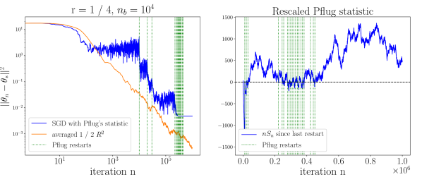
Figure 1: Least-squares on synthetic data. Left: least-squares regression. Right: Scaled Pflug’s statistic $nS_{n}$. The dashed vertical lines correspond to Pflug’s restarts. Note that only the left plot is in log-log scale.

Logistic regression setting.

We consider the objective $f(\theta)=\mathbb{E}\left[\log(1+e^{-y_{i}\langle x_{i},\ \theta\rangle}\right]$. The inputs $x_{i}$ are generated the same way as in the least-square setting. The outputs $y_{i}\in\{-1,1\}$ are generated following the logistic probabilistic model. We use averaged-SGD with step-sizes $\gamma_{n}=1/\sqrt{n}$ as a baseline since it enjoys the optimal rate $O(1/n)$ (Bach, 2014). We also compare to online-Newton (Bach & Moulines, 2013) which achieves better performance in practice.

ResNet18.

We train an 18-layer ResNet model (He et al., 2016) on the CIFAR-10 dataset (Krizhevsky, 2009) using SGD with a momentum of $0.9$, weight decay of $0.0001$ and batch size of $128$. To adapt the distance-based step-size statistic to this scenario, we use Pytorch’s ReduceLROnPlateau() scheduler, created to detect saturation of arbitrary quantities. We use it to reduce the learning rate by a factor $r=0.1$ when it detects that $\left\lVert\theta_{n}-\theta_{restart}\right\rVert^{2}$ has stopped increasing. The parameters of the scheduler are set to: $\text{patience}=1000$, $\text{threshold}=0.01$. Investigating if this choice of parameters is robust to different problems and architectures would be a fruitful avenue for future research. We compare our method to different step-size sequences where the step size is decreased by a factor $r=0.1$ at various epoch milestones. Such sequences achieve state-of-the-art performances when the decay milestones are properly tuned. All initial step sizes are set to $0.1$.

Inefficiency of Pflug’s statistic.

In order to test Pflug’s diagnostic we consider the least-squares setting with $n=1\text{e}6$, $d=20$, $\sigma^{2}=1$. Algorithm 3 is implemented with a conservative burn-in time of $n_{b}=1\text{e}4$ and Algorithm 1 with a discount factor $r=1/4$. We note in Fig. 1 that the algorithm is restarted too often and abusively. This leads to small step sizes early on and to insignificant decrease of the loss afterward. The signal of Pflug’s statistic is very noisy, and its sign gives no significant information on weather saturation has been reached or not. As a consequence the final step-size is very close to 0. We note that its behavior is alike the one of a random walk. On the contrary, averaged-SGD exhibits an $O(1/n)$ convergence rate. We provide further experiments on Pflug’s statistic in Subsection A.1, showing its systematic failure for several values of the decay parameter $r$, the seed and the burn-in.

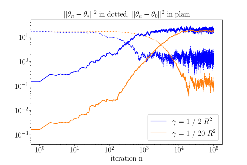
Figure 2: Logistic regression on synthetic dataset. $\left\lVert\theta_{n}-\theta^{*}\right\rVert^{2}$ (dotted) and $\left\lVert\theta_{n}-\theta_{0}\right\rVert^{2}$ (plain) for $2$ different step sizes.

Efficiency of the distance-based diagnostic.

In order to illustrate the benefit of the distance-based diagnostic, we performed extensive experiments in several settings, more precisely: (1) Least Squares regression on a synthetic dataset, (2) Logistic regression on both synthetic and real data, (3) Uniformly convex functions, (4) SVM, (5) Lasso. In all these settings, without any tuning, we achieve the same performance as the best suited method for the problem. These experiments are detailed in Subsection A.2. We hereafter present results for Logistic Regression.

First, we consider the logistic regression setting with $n=1\text{e}5$, $d=20$. In Fig. 2, we compare the behaviour of $\left\lVert\theta_{n}-\theta_{0}\right\rVert^{2}$ and $\left\lVert\theta_{n}-\theta^{*}\right\rVert^{2}$ for two different step sizes $1/2R^{2}$ and $1/20R^{2}$. We first note that these two quantities have the same general behavior: $\left\lVert\theta_{n}-\theta_{0}\right\rVert^{2}$ stops increasing when $\left\lVert\theta_{n}-\theta^{*}\right\rVert^{2}$ starts to saturate, and that this observation is consistent for the two step sizes. We additionally note that the average slope of $\left\lVert\theta_{n}-\theta_{0}\right\rVert^{2}$ is of value $2$ during the transient phase and of value $0$ when stationarity has been reached. This demonstrates that, even if this diagnostic is inspired by the quadratic case, the main conclusions of Corollary 15 still hold for convex non-quadratic function and the distance-based diagnostic in Algorithm 4 should be more generally valid. We also notice that the two oracle restart times are spaced by $\log(20/2)=1$ which confirms that the transient phase lasts $\Theta(1/\gamma)$.

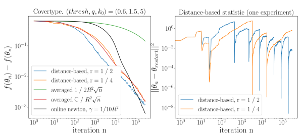
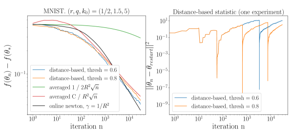
Figure 3: Top: Covertype dataset. Two different values of $r$ are used: $1/2$, $1/4$. Bottom: MNIST dataset. Two different values of $thresh$ are used: $0.6$, $0.8$. Left: Logistic regression. Right: distance-based statistics $\left\lVert\theta_{n}-\theta_{restart}\right\rVert^{2}$.

We further investigate the performance of the distance-based diagnostic on real-world datasets: the Covertype dataset and the MNIST dataset. Each dataset is divided in two equal parts, one for training and one for testing. We then sample without replacement and perform a total of one pass over all the training samples. The loss is computed on the test set. This procedure is replicated $10$ times and the results are averaged. For MNIST the task consists in classifying the parity of the labels which are $\{0,\dots,9\}$. We compare our algorithm to: online-Newton ($\gamma=1/10R^{2}$ for the Covertype dataset and $\gamma=1/R^{2}$ for MNIST) and averaged-SGD with step sizes $\gamma_{n}=1/2R^{2}\sqrt{n}$ (the value suggested by theory) and $\gamma_{n}=C/\sqrt{n}$ (where the parameter $C$ is tuned to achieve the best testing error). In Fig. 3, we present the results. Top row corresponds to the Covertype dataset for two different values of the decrease coefficient $r=1/2$ and $r=1/4$, the other parameters are set to $(tresh,q,k_{0})=(0.6,1.5,5)$, left are shown the convergence rates for the different algorithms and parameters, right are plotted the evolution of the distance-based statistic $\left\lVert\theta_{n}-\theta_{0}\right\rVert^{2}$. Bottom row corresponds to the MNIST dataset for two different values of the threshold $thresh=0.6$ and $thresh=0.8$, the other parameters are set to $(r,q,k_{0})=(1/2,1.5,5)$, left are shown the convergence rates for the different algorithms and parameters, right are plotted the evolution of the distance-based statistic $\left\lVert\theta_{n}-\theta_{0}\right\rVert^{2}$. The initial step size for our distance-based algorithm was set to $4/R^{2}$. Our adaptive algorithm obtains comparable performance as online-Newton and optimally-tuned averaged SGD, enjoying a convergence rate $O(1/n)$, and better performance than theoretically-tuned averaged-SGD. Moreover we note that the convergence of the distance-based algorithm is the fastest early stage. Thus this algorithm seems to benefit from the same exponential-forgetting of initial conditions as the oracle diagnostic (see Proposition 6). We point out that our algorithm is relatively independent of the choice of $r$ and $thresh$. We also note (red and green curves) that the theoretically optimal step size is outperformed by the hand-tuned one with the same decay, which only confirms the need for adaptive methods. On the right is plotted the statistic during the SGD procedure. Unlike Pflug’s one, the signal is very clean, which is mostly due to the large range of values that are taken.

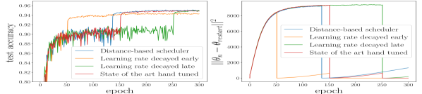
Figure 4: ResNet18 trained on Cifar10. Left: test accuracies. Right: distance-based statistic $\left\lVert\theta_{n}-\theta_{restart}\right\rVert^{2}$.

Application to deep learning.

We conclude by testing the distance-based statistic on a deep-learning problem in Fig. 4. In practice, the learning rate is decreased when the accuracy has stopped increasing for a certain number of epochs. In red is plotted the accuracy curve obtained when the learning rate is decreased by a factor $r=0.1$ at epochs $150$ and $250$. These specific epochs have been manually tuned to obtain state of the art performance.

Looking at the red accuracy curve, it seems natural to decrease the learning rate earlier around epoch $50$ when the test accuracy has stopped increasing. However doing so leads to a lower final accuracy (orange curve). On the other hand, decreasing the learning rate later, at epoch $250$, leads to a good final accuracy but takes longer to reach it. If instead of paying attention to the test accuracy we focus on the metric $\left\lVert\theta_{n}-\theta_{restart}\right\rVert^{2}$ we notice that it still notably increases after epoch $50$ and until epoch $150$. This phenomenon manifests that this statistic contains information that cannot be simply obtained from the test accuracy curve. Hence when the ReduceLROnPlateau scheduler is implemented using the distance-based strategy, the learning rate is automatically decreased around epoch $140$ and kept constant beyond (blue curve) which leads to a final state-of-the-art accuracy.

Therefore our distance-based statistic seems also to be a promising tool to adaptively set the step size for deep learning applications. We hope this will inspire further research.

Conclusion

In this paper we studied convergence-diagnostic step-sizes. We first showed that such step-sizes make sense in the smooth and strongly convex framework since they recover the optimal $O(1/n)$ rate with in addition an exponential decrease of the initial conditions. Two different convergence diagnostics are then analysed. First, we theoretically prove that Pflug’s diagnostic leads to abusive restarts in the quadratic case. We then propose a novel diagnostic which relies on the distance of the final iterate to the restart point. We provide a simple restart criterion and theoretically motivate it in the quadratic case. The experimental results on synthetic and real world datasets show that our simple diagnostic leads to very satisfying convergence rates in a variety of frameworks.

An interesting future direction to our work would be to theoretically prove that our diagnostic leads to adequate restarts, as seen experimentally. It would also be interesting to explore more in depth the applications of our diagnostic in the non-convex framework.

Organization of the Appendix

In the appendix, we provide additional experiments and detailed proofs to all the results presented in the main paper.

1. In Appendix A we provide additional experiments. In Subsection A.1 we show that Pflug’s diagnostic fails for different values of decrease factor $r$ and burn-in time $n_{b}$; together with a simple experimental illustration of Proposition 13. Then in Subsection A.2 we investigate the performance of the distance-based statistic in different settings and for different values of $r$ and of the threshold value $thresh$. These settings are: Least-squares, Logistic regression, SVM, Lasso regression, and the Uniformly convex setting.

2. In Appendix B we prove Proposition 6 as well as a similar result for uniformly convex functions.

3. In Appendix C we prove Proposition 9 and Proposition 13 .

4. Finally in Appendix D we prove Proposition 14 and Corollary 15.

Appendix A Supplementary experiments

Here we provide additional experiments for the Pflug diagnostic and the distance-based statistic in different settings.

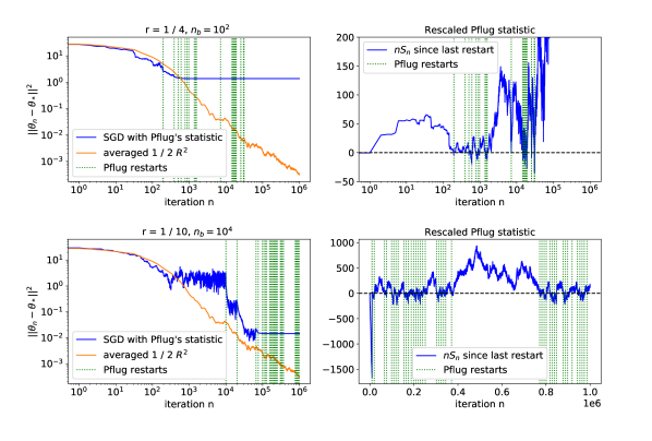
Figure 5: Least-squares on synthetic data ($n=1\text{e}6$, $d=20$, $\sigma^{2}=1$). Left: least-squares regression. Right: Scaled Pflug statistic $nS_{n}$. The dashed vertical lines correspond to Pflug’s restarts. Note that the x-axis of the bottom right plot is not in log scale. Top parameters: $r=1/10$, $n_{b}=10^{4}$. Bottom parameters: $r=1/4$, $n_{b}=10^{2}$. Initial learning rates set to $1/2R^{2}$.

A.1 Supplementary experiments on Pflug’s diagnostic

We test Pflug’s diagnostic in the least-squares setting with $n=1\text{e}6$, $d=20$, $\sigma^{2}=1$, $\gamma_{0}=1/2R^{2}$. Notice that as in Fig. 1, Plug’s diagnostic fails for different values of the algorithm’s parameters. Indeed parameters $(r,n_{b})=(1/4,10^{2})$ (Fig. 5 top row) and $(r,n_{b})=(1/10,10^{4})$ (Fig. 5 bottom row) both lead to abusive restarts (dotted vertical lines) that do not correspond to iterate saturation. These restarts lead to small step size too early and insignificant progress of the loss afterwards. Notice that in both cases the behaviour of the rescaled statistic $nS_{n}$ is similar to a random walk. On the contrary, as the theory suggests (Bach & Moulines, 2013) averaged-SGD exhibits a $O(1/n)$ convergence rate.

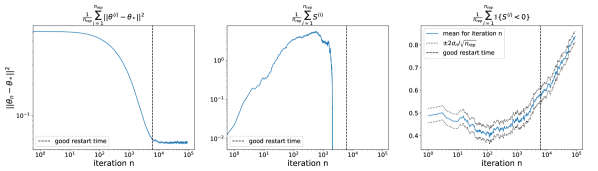
Figure 6: Least-squares on synthetic data ($n=1\text{e}5$, $d=20$, $\sigma^{2}=1$). Parameters: $\gamma_{\text{old}}=1/5R^{2}$, $r=1/10$, $n_{rep}=10^{3}$. Left: least-squares regression averaged over all $n_{rep}$ samples. Middle: average of Pflug’s statistic over all $n_{rep}$ samples. Right: fraction of runs where the statistic is negative at iteration $n$. The two dotted lines roughly correspond to the $95\%$ confidence intervals.

In order to illustrate Proposition 13 in the least-squares framework, we repeat $n_{rep}$ times the same experiment which consists in running constant step-size SGD from an initial point $\theta_{0}\sim\pi_{\gamma_{\text{old}}}$ with a smaller step-size $\gamma=r\times\gamma_{\text{old}}$. The starting point $\theta_{0}\sim\pi_{\gamma_{\text{old}}}$ is obtained by running for a sufficiently long time SGD with constant step size $\gamma_{\text{old}}$. In Fig. 6 we implement these multiple experiments with $n=1\text{e}5$, $d=20$, $\sigma^{2}=1$. In the left plot notice the two characteristic phases: the exponential decrease of $\left\lVert\theta_{n}-\theta^{*}\right\rVert$ followed by the saturation of the iterates, the good restart time corresponding to this transition is indicated by the black dotted vertical line. Consistent with Proposition 9, we see in the middle plot that in expectation Pflug’s statistic is positive then negative (the curve disappears as soon as its value is negative due to the plot in log-log scale). This change of sign occurs roughly at the same time as when the iterates saturate. However, in the right graph we plot for each iteration $k$ the fraction of runs for which the statistic $S_{k}$ is negative. We see that this fraction is close to $0.5$ for all $k$ smaller than the good restart time. Since for $n_{rep}$ big enough $\frac{1}{n_{rep}}\sum_{i=1}^{n_{rep}}\mathbbm{1}\{S_{k}^{(i)}<0\}\sim\mathbb{P}(S_{k}^{(i)}<0)$, this is an illustration of Proposition 13. Hence whatever the burn-in $n_{b}$ fixed by Pflug’s algorithm, there is a chance out of two of restarting too early.

A.2 Supplementary experiments on the distance-based diagnostic

In this section we test our distance-based diagnostic in several settings.

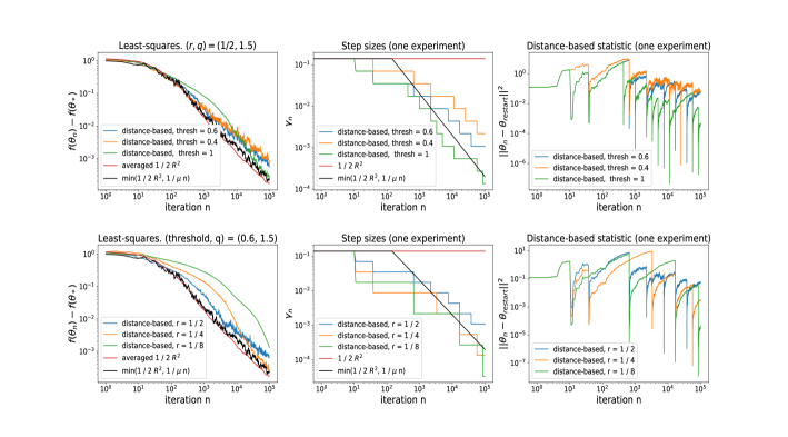
Figure 7: Least-squares on synthetic data ($n=1\text{e}5$, $d=20$, $\sigma^{2}=1$). All initial step sizes of $1/2R^{2}$. Top distanced-based parameters: $(r,q,k_{0})=(1/2,0.5,5)$. Bottom distanced-based parameters: $(thresh,q,k_{0})=(0.6,1.5,5)$. The losses on the left plot are averaged over $10$ replications.

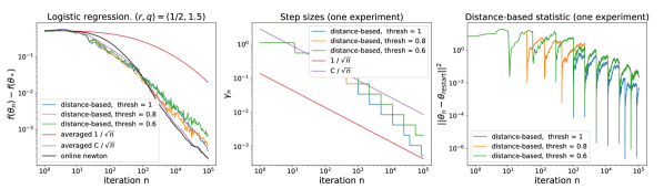
Figure 8: Logistic regression on synthetic data ($n=1\text{e}5$, $d=20$). Distanced-based parameters: $(r,q,k_{0})=(1/2,1.5,5)$ and $\gamma_{0}=4/R^{2}$. The losses on the left plot are averaged over $10$ replications.

Least-squares regression.

We consider the objective $f(\theta)=\frac{1}{2}\mathbb{E}\left[(y-\langle x,\ \theta\rangle)^{2}\right]$. The inputs $x_{i}$ are i.i.d. from $\mathcal{N}(0,H)$ where $H$ has random eigenvectors and eigenvalues $(1/k)_{1\leq k\leq d}$. We note $R^{2}=\operatorname{Tr}\ H$. The outputs $y_{i}$ are generated following the generative model $y_{i}=\langle x_{i},\ \theta^{*}\rangle+\varepsilon_{i}$ where $(\varepsilon_{i})_{1\leq i\leq n}$ are i.i.d. from $\mathcal{N}(0,\sigma^{2})$. We test the distance-based strategy with different values of the threshold $thresh\in\{0.4,0.6,1\}$ and of the decrease factor $r\in\{1/2,1/4,1/8\}$. We use averaged-SGD with constant step size $\gamma=1/2R^{2}$ as a baseline since it enjoys the optimal statistical rate $O(\sigma^{2}d/n)$ (Bach & Moulines, 2013), we also plot SGD with step size $\gamma_{n}=1/\mu n$ which achieves a rate of $1/\mu n$.

We observe in Fig. 7 that the distance-based strategy achieves similar performances as $1/\mu n$ step sizes without knowing $\mu$. Furthermore the performance does not heavily depend on the values of $r$ and $thresh$ used. In the middle plot of Fig. 7 notice how the distance-based step-sizes mimic the $1/\mu n$ sequence. We point out that the performance of constant-step-size averaged SGD and $1/\mu n$-step-size SGD are comparable since the problem is fairly well conditioned ($\mu=1/20$).

Logistic regression.

We consider the objective $f(\theta)=\mathbb{E}\left[\log(1+e^{-y\langle x,\ \theta\rangle})\right]$. The inputs $x_{i}$ are generated the same way as in the least-square setting. The outputs $y_{i}$ are generated following the logistic probabilistic model $y_{i}\sim\mathcal{B}((1+\exp(-\langle x_{i},\ \theta^{*}\rangle)^{-1})$. We use averaged-SGD with step-sizes $\gamma_{n}=1/\sqrt{n}$ as a baseline since it enjoys the optimal rate $O(1/n)$ (Bach, 2014). We also compare to online-Newton (Bach & Moulines, 2013) which achieves better performance in practice and to averaged-SGD with step-sizes $\gamma_{n}=C/\sqrt{n}$ where parameter $C$ is tuned in order to achieve best performance.

In Fig. 8 notice how averaged-SGD with the theoretical step size $\gamma_{n}=1/\sqrt{n}$ performs poorly. However once the parameter $C$ in $\gamma_{n}=C/\sqrt{n}$ is tuned properly averaged-SGD and online Newton perform similarly. Note that our distance-based strategy with $r=1/2$ achieves similar performances which do not heavily depend on the value of the threshold $thresh$.

SVM.

We consider the objective $f(\theta)=\mathbb{E}\left[\max(0,1-y\langle x,\ \theta\rangle)\right]+\frac{\lambda}{2}\left\lVert\theta\right\rVert^{2}$ where $\lambda>0$. Note that $f$ is strongly-convex with parameter $\lambda$ and non-smooth. The inputs $x_{i}$ are generated i.i.d. from $\mathcal{N}(0,\eta^{2}I_{d})$. The outputs $y_{i}$ are generated as $y_{i}=\text{sgn}(x_{i}(1)+z_{i})$ where $z_{i}\sim\mathcal{N}(0,\sigma^{2})$. We generate $n=1\text{e}5$ points in dimension $d=20$. We compare our distance-based strategy with different values of the threshold $thresh\in\{0.6,0.8,1\}$ to averaged-SGD with step sizes $\gamma_{n}=1/\mu n$ which achieves the rate of $\log n/\mu n$ (Lacoste-Julien et al., 2012) and averaged-SGD with step sizes $\gamma_{n}=C/\sqrt{n}$ where $C$ is tuned in order to achieve best performance.

In Fig. 9 note that averaged-SGD with $\gamma_{n}=1/\mu n$ exhibits a $O(1/n)$ rate but the initial values are bad. On the other hand, once properly tuned, averaged SGD with $\gamma_{n}=C/\sqrt{n}$ performs very well, similarly as in the smooth setting. Note that our distance-based strategy with $r=1/2$ achieves similar performances which do not depend on the value of the threshold $thresh$.

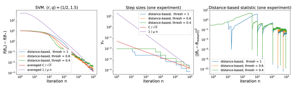
Figure 9: SVM on synthetic data ($n=1\text{e}5$, $d=20$, $\lambda=0.1$, $\eta^{2}=25$ and $\sigma=1$). Distanced-based parameters: $(r,q,k_{0})=(1/2,1.5,5)$ and $\gamma_{0}=4/R^{2}$. The losses on the left plot are averaged over $10$ replications.

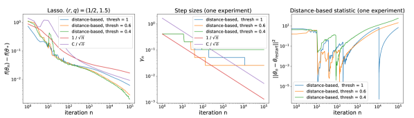
Figure 10: Lasso regression on synthetic data ($\text{number of iterations}=1\text{e}5$, $n=80$, $d=100$, $s=60$, $\sigma=0.1$, $\lambda=10^{-4}$). Initial step-sizes of $1/2R^{2}$ (except for the tuned $C/\sqrt{n}$). Distanced-based parameters: $(r,q,k_{0})=(1/2,1.5,5)$. The losses on the left plot are averaged over $10$ replications.

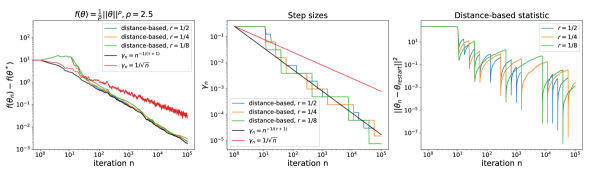
Figure 11: Uniformly convex function $f(\theta)=\frac{1}{\rho}\left\lVert\theta\right\rVert_{2}^{\rho}$ ($n=1\text{e}5$, $d=200$, $\rho=2.5$). Initial step size of $\gamma_{0}=1/4L$ for all step-size sequences. Distance-based parameters $(thresh,q,k_{0})=(1,1.5,5)$. The losses on the left plot correspond to only one replication.

Lasso Regression.

We consider the objective $f(\theta)=\frac{1}{n}\sum_{i=1}^{n}(y_{i}-\langle x_{i},\ \theta\rangle)^{2}+\lambda\left\lVert\theta\right\rVert_{1}$. The inputs $x_{i}$ are i.i.d. from $\mathcal{N}(0,H)$ where $H$ has random eigenvectors and eigenvalues $(1/k^{3})_{1\leq k\leq d}$. We choose $n=80$, $d=100$. We note $R^{2}=\operatorname{Tr}\ H$. The outputs $y_{i}$ are generated following $y_{i}=\langle x_{i},\ \tilde{\theta}\rangle+\varepsilon_{i}$ where $(\varepsilon_{i})_{1\leq i\leq n}$ are i.i.d. from $\mathcal{N}(0,\sigma^{2})$ and $\tilde{\theta}$ is an $s$-sparse vector. Note that $f$ is non-smooth and the smallest eigenvalue of $H$ is $1/10^{6}$, hence for the number of iterations we run SGD $f$ cannot be considered as strongly convex. We compare the distance-based strategy with different values of the threshold $thresh\in\{0.4,0.6,1\}$ to SGD with step-size sequence $\gamma_{n}=1/\sqrt{n}$ which achieves a rate of $\log n/\sqrt{n}$ (Shamir & Zhang, 2013) and to step-size sequence $\gamma_{n}=C/\sqrt{n}$ where $C$ is tuned to achieve best performance. Let us point out that the purpose of this experiment is to investigate the performance of the distance-based statistic on non-smooth problems and therefore we use as baseline generic algorithms for non-smooth optimization – even though, in the special case of the Lasso regression, there exists first-order proximal algorithms which are able to leverage the special structure of the problem and obtain the same performance as for smooth optimization (Beck & Teboulle, 2009).

In Fig. 10 note that SGD with the theoretical step-size sequence $\gamma_{n}=1/\sqrt{n}$ performs poorly. Tuning the parameter $C$ in $\gamma_{n}=C/\sqrt{n}$ improves the performance. However our distance-based strategy with $r=1/2$ performs better for several different values of $thresh$.

Uniformly convex $f$.

We consider the objective $f(\theta)=\frac{1}{\rho}\left\lVert\theta\right\rVert_{2}^{\rho}$ where $\rho=2.5$. Notice that $f$ is not strongly convex but is uniformly convex with parameter $\rho$ (see Assumption 16). We generate the noise on the gradients $\xi_{i}$ as i.i.d from $\mathcal{N}(0,I_{d})$. We compare the distance-based strategy with different values of the decrease factor $r\in\{1/2,1/4,1/8\}$ to SGD with step-size sequence $\gamma_{n}=1/\sqrt{n}$ which achieves a rate of $\log n/\sqrt{n}$ (Shamir & Zhang, 2013) and to SGD with step size $\gamma_{n}=n^{-1/(\tau+1)}$ ($\tau=1-2/\rho$) which we expect to achieve a rate of $O(n^{-1/(\tau+1)}\log n)$ (see remark after Corollary 19). Notice in Fig. 11 how the distance-based strategy achieves the same rate as SGD with step-sizes $\gamma_{n}=n^{-1/(\tau+1)}$ without knowing parameter $\tau$. Furthermore the performance does not depend on the value of $r$ used. In the middle plot of Fig. 7 notice how the distance-based step sizes mimic the $n^{-1/(\tau+1)}$ sequence.

Therefore the distance-based diagnostic works in a variety of settings where it automatically adapts to the problem difficulty without having to know the specific parameters (such as strong-convexity or uniform-convexity parameters).

Appendix B Performance of the oracle diagnostic

In this section, we prove the performance of the oracle diagnostic in the strongly-convex setting and consider its extension to the uniformly-convex setting.

B.1 Proof of Proposition 6

We first introduce some notations which are useful in the following analysis.

Notation.

For $k\geq 1$, let $n_{k+1}$ be the number of iterations until the $(k+1)^{th}$ restart and $\Delta n_{k+1}$ be the number of iterations between the restart $k$ and restart $(k+1)$ during which step size $\gamma_{k}$ is used. Therefore we have that $n_{k}=\sum_{k^{\prime}=1}^{k}\Delta n_{k^{\prime}}$. We also denote by $\delta_{n}=\mathbb{E}\left[\left\lVert\theta_{n}-\theta^{*}\right\rVert^{2}\right]$.

Notice that for $n\geq 1$ and $|x|\leq n$ it holds that $(1-x)^{n}\leq\exp(-nx)$. Hence Proposition 5 leads to:

$$\mathbb{E}\left[\left\lVert\theta_{n}-\theta^{*}\right\rVert^{2}\right] \leq(1-\gamma\mu)^{n}\delta_{0}+\frac{2\sigma^{2}}{\mu}\gamma$$ (2)

$$\leq\exp(-n\gamma\mu)\delta_{0}+\frac{2\sigma^{2}}{\mu}\gamma.$$ (3)

In order to simplify the computations, we analyse Algorithm 2 with the bias-variance trade-off stated in eq. 3 instead of the one of eq. 2. Note however that it does not change the result. We prove separately the results obtained before and after the first restart $\Delta n_{1}$.

Before the first restart.

Let $\theta_{0}\in\mathbb{R}^{d}$. For $n\leq\Delta n_{1}=n_{1}$ (first restart time) we have that:

$$\mathbb{E}\left[\left\lVert\theta_{n}-\theta^{*}\right\rVert^{2}\right] \leq\exp(-n\gamma_{0}\mu)\delta_{0}+\frac{2\sigma^{2}}{\mu}\gamma_{0}.$$ (4)

Following the oracle strategy, the restart time $\Delta n_{1}$ corresponds to $\exp(-\Delta n_{1}\gamma_{0}\mu)\delta_{0}=\frac{2\sigma^{2}}{\mu}\gamma_{0}$. Hence $\Delta n_{1}=\frac{1}{\gamma_{0}\mu}\ln\left(\frac{\mu\delta_{0}}{2\gamma_{0}\sigma^{2}}\right)$ and $\delta_{n_{1}}\leq\exp(-\Delta n_{1}\gamma_{0}\mu)\delta_{0}+\frac{2\sigma^{2}}{\mu}\gamma_{0}=\frac{4\sigma^{2}}{\mu}\gamma_{0}$.

After the first restart.

Let $k\geq 1$ and $n_{k}\leq n\leq n_{k+1}$. We obtain from eq. 3:

$$\mathbb{E}\left[\left\lVert\theta_{n}-\theta^{*}\right\rVert^{2}\right] \leq\exp(-(n-n_{k})\gamma_{k}\mu)\mathbb{E}\left[\left\lVert\theta_{n_{k}}-\theta^{*}\right\rVert^{2}\right]+\frac{2\sigma^{2}}{\mu}\gamma_{k}.$$

The oracle construction of the restart time leads to:

$$\exp(-\Delta n_{k+1}\gamma_{k}\mu)\delta_{n_{k}}=\frac{2\sigma^{2}}{\mu}\gamma_{k}.$$

Which yields

$$\Delta n_{k+1} =\frac{1}{\gamma_{k}\mu}\ln{\frac{\mu\delta_{n_{k}}}{2\sigma^{2}\gamma_{k}}}.$$

However we know by construction that for $k\geq 1$, $\delta_{n_{k}}\leq\exp(-\Delta n_{k}\gamma_{k-1}\mu)\delta_{n_{k-1}}+\frac{2\sigma^{2}}{\mu}\gamma_{k-1}=\frac{4\sigma^{2}}{\mu}\gamma_{k-1}$. Hence:

$$\Delta n_{k+1} \leq\frac{1}{\gamma_{k}\mu}\ln 2\frac{\gamma_{k-1}}{\gamma_{k}}.$$

Considering that $\gamma_{k}=r^{k}\gamma_{0}$,

$$\Delta n_{k+1} \leq\frac{1}{r^{k}\gamma_{0}\mu}\ln\frac{2}{r}.$$

Since $n_{k}=\Delta n_{1}+\sum_{k^{\prime}=2}^{k}\Delta n_{k^{\prime}}$ we have that

$$n_{k}-\Delta n_{1}=\sum_{k^{\prime}=2}^{k}\Delta n_{k^{\prime}} \leq\frac{1}{\mu\gamma_{0}}\ln\left(\frac{2}{r}\right)\sum_{k^{\prime}=2}^{k}\frac{1}{r^{k^{\prime}-1}}$$

$$\leq\frac{1}{\mu\gamma_{0}}\ln\left(\frac{2}{r}\right)\sum_{k^{\prime}=1}^{k}\frac{1}{r^{k^{\prime}-1}}$$

$$\leq\frac{1}{\mu\gamma_{0}(1-r)}\ln\left(\frac{2}{r}\right)\frac{1}{r^{k-1}}$$

$$=\frac{1}{\mu(1-r)\gamma_{k-1}}\ln\left(\frac{2}{r}\right).$$

Therefore since $\delta_{n_{k}}\leq\frac{4\sigma^{2}}{\mu}\gamma_{k-1}$ we get:

$$\delta_{n_{k}}\leq\frac{4\sigma^{2}}{(n_{k}-\Delta n_{1})\mu^{2}(1-r)}\ln{\Big{(}\frac{2}{r}\Big{)}}.$$ (5)

We now want a result for any $n$ and not only for restart times. For $n\leq n_{1}=\Delta n_{1}$ we are done using eq. 4. For $k\geq 1$, let $n_{k}\leq n\leq n_{k+1}$, from Proposition 5 and eq. 5 we have that:

$$\delta_{n} \leq\exp(-(n-n_{k})\gamma_{k}\mu)\delta_{n_{k}}+\frac{2\gamma_{k}\sigma^{2}}{\mu}$$

$$\leq\exp(-(n-n_{k})\gamma_{k}\mu)\frac{A}{n_{k}-\Delta n_{1}}+\frac{2\gamma_{k}\sigma^{2}}{\mu},$$

where $A=\frac{4\sigma^{2}}{\mu^{2}(1-r)}\ln{\Big{(}\frac{2}{r}\Big{)}}$. Let $g(n)=\exp(-(n-n_{k})\gamma_{k}\mu)\frac{A}{n_{k}-\Delta n_{1}}+\frac{2\gamma_{k}\sigma^{2}}{\mu}$ and $h(n)=\frac{A}{n-\Delta n_{1}}+\frac{2\gamma_{k}\sigma^{2}}{\mu}$ for $n>\Delta n_{1}$. Note that $g$ is exponential, $h$ is an inverse function and that $g(n_{k})=h(n_{k})$. This implies that that for $n\geq n_{k}$, $g(n)\leq h(n)$. Hence for $n\geq n_{k}$:

$$\delta_{n} \leq\frac{A}{n-\Delta n_{1}}+\frac{2\gamma_{k}\sigma^{2}}{\mu}$$

$$\leq\frac{A}{n-\Delta n_{1}}+\frac{4\gamma_{k}\sigma^{2}}{\mu}.$$

By construction, $\frac{4\sigma^{2}}{\mu}\gamma_{k}\leq\frac{A}{n_{k+1}-\Delta n_{1}}$. However since $\frac{A}{n_{k+1}-\Delta n_{1}}\leq\frac{A}{n-\Delta n_{1}}$ for $n\leq n_{k+1}$ we get that $\frac{4\sigma^{2}}{\mu}\gamma_{k}\leq\frac{A}{n-\Delta n_{1}}$ for $n\leq n_{k+1}$. Hence for $n_{k}\leq n\leq n_{k+1}$ and therefore for all $n>\Delta n_{1}$:

$$\delta_{n} \leq\frac{2A}{n-\Delta n_{1}}$$

$$\leq\frac{8\sigma^{2}}{\mu^{2}(n-\Delta n_{1})(1-r)}\ln{\Big{(}\frac{2}{r}\Big{)}}.$$

This concludes the proof. Note that this upper bound diverges for $r\to 0\ \text{or}\ 1$ and could be minimized over the value of $r$.

B.2 Uniformly convex setting

The previous result holds for smooth strongly-convex functions. Here we extend this result to a more generic setting where $f$ is not supposed strongly convex but uniformly convex.

Assumption 16 (Uniform convexity).

There exists finite constants $\mu>0,\rho>2$ such that for all $\theta,\eta\in\mathbb{R}^{d}$ and any subgradient $f^{\prime}(\eta)$ of $f$ at $\eta$:

$$f(\theta)\geq f(\eta)+\langle f^{\prime}(\eta),\ \theta-\eta\rangle+\frac{\mu}{\rho}\left\lVert\theta-\eta\right\rVert^{\rho}.$$

This assumption implies the convexity of the function $f$ and the definition of strong convexity is recovered for $\rho\to 2$. It also recovers the definition of weak-convexity around $\theta^{*}$ when $\rho\to+\infty$ since $\textstyle\lim_{\rho\to+\infty}\frac{\mu}{\rho}\left\lVert\theta-\theta^{*}\right\rVert^{\rho}=0$ for $\left\lVert\theta-\theta^{*}\right\rVert\leq 1$.

To simplify our presentation and as is often done in the literature we restrict the analysis to the constrained optimization problem:

$$\min_{\theta\in\mathcal{W}}f(\theta),$$

where $\mathcal{W}$ is a compact convex set and we assume $f$ attains its minimum on $\mathcal{W}$ at a certain $\theta_{*}\in\mathbb{R}^{d}$. We consider the projected SGD recursion:

$${}\theta_{i+1}=\Pi_{\mathcal{W}}\left[\theta_{i}-\gamma_{i+1}f^{\prime}_{i+1}(\theta_{i})\right].$$ (6)

We also make the following assumption (which does not contradict Assumption 16 in the constrained setting).

Assumption 17 (Bounded gradients).

There exists a finite constant $G>0$ such that

$$\mathbb{E}\left[\left\lVert f^{\prime}_{i}(\theta)\right\rVert^{2}\right]\leq G^{2}$$

for all $i\geq 0$ and $\theta\in\mathcal{W}$.

In order to obtain a result similar to Proposition 6 but for uniformly convex functions, we first need to analyse the behaviour of constant step-size SGD in this new framework and obtain a classical bias-variance trade off similar to Proposition 5.

B.2.1 Constant step-size SGD for uniformly convex functions

The following proposition exhibits the bias-variance trade off obtained for the function values when constant step-size SGD is used on uniformly convex functions.

Proposition 18.

Consider the recursion in eq. 6 under Assumptions 1, 17 and 16. Let $\tau=1-\frac{2}{\rho}\in(0,1)$, $q=(\frac{1}{\tau}-1)^{-1}$, $\tilde{\mu}=4\frac{\mu}{\rho}$ and $\delta_{0}=\mathbb{E}\left[\|\theta_{0}-\theta^{*}\|^{2}\right]$. Then for any step-size $\gamma>0$ and time $n\geq 0$ we have:

$$\mathbb{E}\left[f(\theta_{n})\right]-f(\theta^{*})\leq\frac{\delta_{0}}{\gamma n\left(1+nq\gamma\tilde{\mu}\delta_{0}^{q}\right)^{\frac{1}{q}}}+\gamma G^{2}(1+\log n).$$

Note that the bias term decreases at a rate $n^{-1/\tau}$ which is an interpolation of the rate obtained when $f$ is strongly convex ($\tau\to 0$, exponential decrease of bias) and when $f$ is simply convex ($\tau=1$, bias decrease rate of $n^{-1}$). This bias-variance trade off directly implies the following rate in the finite horizon setting.

Corollary 19.

Consider the recursion in eq. 6 under Assumptions 1, 17 and 16. Then for a finite time horizon $N\geq 0$ and constant step size $\gamma=N^{-\frac{1}{\tau+1}}$ we have:

$$\mathbb{E}\left[f(\theta_{N})\right]-f(\theta^{*})=O\left(N^{-\frac{1}{1+\tau}}\log N\right).$$

Remarks.

When the total number of iterations $N$ is fixed, Juditsky & Nesterov (2014) find a similar result as Corollary 19 for minimizing uniformly convex functions. However their algorithm uses averaging and multiple restarts. In the deterministic framework, using a weaker but similar assumption as uniform convexity, Roulet & d’Aspremont (2017) obtain a similar $O(N^{-\frac{1}{\tau}})$ convergence rate for gradient descent for smooth uniformly convex functions. This is coherent with the bias variance trade off we get and Corollary 19 extends their result to the stochastic framework. We also note that the result in Corollary 19 holds only in the fixed horizon framework, however we believe that this rate still holds when using a decreasing step size $\gamma_{n}=n^{-\frac{1}{\tau+1}}$. The analysis is however much harder since it requires analysing the recursion stated in Subsection B.2.2 with a decreasing step-size sequence.

Hence Corollary 19 shows that an accelerated rate of $O\left(\log(n)n^{-\frac{1}{1+\tau}}\right)$ is obtained with appropriate step sizes. However in practice the parameter $\rho$ is unknown and this step size sequence cannot be implemented. In Subsection B.2.3 we show that we can bypass $\rho$ by using the oracle restart strategy. In the following subsection Subsection B.2.2 we prove Proposition 18 and Corollary 19.

B.2.2 Proof of Proposition 18 and Corollary 19

We start by stating the following lemma directly inspired by Shamir & Zhang (2013).

Lemma 20.

Under Assumptions 1 and 17. Consider projected SGD in eq. 6 with constant step size $\gamma>0$. Let $1\leq p\leq n$ and denote $S_{p}=\frac{1}{p+1}\sum_{i=n-p}^{n}f(\theta_{i})$, then:

$$\mathbb{E}\left[f(\theta_{n})\right]\leq\mathbb{E}\left[S_{p}\right]+\frac{\gamma}{2}G^{2}(\log(p)+1).$$

Proof.

We follow the proof technique of Shamir & Zhang (2013). The goal is to link the value of the final iterate with the averaged last $p$ iterates. For any $\theta\in\mathcal{W}$ and $\gamma>0$:

$$\theta_{i+1}-\theta=\Pi_{\mathcal{W}}\left[\theta_{i}-\gamma f^{\prime}_{i+1}(\theta_{i})\right]-\theta.$$

By convexity of $\mathcal{W}$ we have the following:

$$\left\lVert\theta_{i+1}-\theta\right\rVert^{2} \leq\left\lVert\theta_{i}-\gamma f^{\prime}_{i+1}(\theta_{i})-\theta\right\rVert^{2}$$

$$=\left\lVert\theta_{i}-\theta\right\rVert^{2}-2\gamma\langle f^{\prime}_{i+1}(\theta_{i}),\ \theta_{i}-\theta\rangle+\gamma^{2}\left\lVert f^{\prime}_{i+1}(\theta_{i})\right\rVert^{2}.$$ (7)

Rearranging we get

$$\langle f^{\prime}_{i+1}(\theta_{i}),\ \theta_{i}-\theta\rangle\leq\frac{1}{2\gamma}\left[\left\lVert\theta_{i}-\theta\right\rVert^{2}-\left\lVert\theta_{i+1}-\theta\right\rVert^{2}\right]+\frac{\gamma}{2}\left\lVert f^{\prime}_{i+1}(\theta_{i})\right\rVert^{2}.$$ (8)

Let $k$ be an integer smaller than $n$. Summing eq. 8 from $i=n-k$ to $i=n$ we get

$$\sum_{i=n-k}^{n}\langle f^{\prime}_{i+1}(\theta_{i}),\ \theta_{i}-\theta\rangle\leq\frac{1}{2\gamma}\left[\left\lVert\theta_{n-k}-\theta\right\rVert^{2}-\left\lVert\theta_{n+1}-\theta\right\rVert^{2}\right]+\frac{\gamma}{2}\sum_{i=n-k}^{n}\left\lVert f^{\prime}_{i+1}(\theta_{i})\right\rVert^{2}.$$

Taking the expectation and using the bounded gradients hypothesis:

$$\sum_{i=n-k}^{n}\mathbb{E}\left[\langle f^{\prime}(\theta_{i}),\ \theta_{i}-\theta\rangle\right] \leq\frac{1}{2\gamma}\mathbb{E}\left[\left\lVert\theta_{n-k}-\theta\right\rVert^{2}-\left\lVert\theta_{n+1}-\theta\right\rVert^{2}\right]+\frac{\gamma}{2}\sum_{i=n-k}^{n}\mathbb{E}\left[\left\lVert f^{\prime}_{i+1}(\theta_{i})\right\rVert^{2}\right]$$

$$\leq\frac{1}{2\gamma}\mathbb{E}\left[\left\lVert\theta_{n-k}-\theta\right\rVert^{2}-\left\lVert\theta_{n+1}-\theta\right\rVert^{2}\right]+\frac{\gamma}{2}(k+1)G^{2}.$$

The function $f$ being convex we have that $f(\theta_{i})-f(\theta)\leq\langle f^{\prime}(\theta_{i}),\ \theta_{i}-\theta\rangle$. Therefore:

$$\frac{1}{k+1}\sum_{i=n-k}^{n}\mathbb{E}\left[f(\theta_{i})-f(\theta)\right] \leq\frac{1}{2\gamma(k+1)}\mathbb{E}\left[\left\lVert\theta_{n-k}-\theta\right\rVert^{2}-\left\lVert\theta_{n+1}-\theta\right\rVert^{2}\right]+\frac{\gamma}{2}G^{2}$$

$$\leq\frac{1}{2\gamma(k+1)}\mathbb{E}\left[\left\lVert\theta_{n-k}-\theta\right\rVert^{2}\right]+\frac{\gamma}{2}G^{2}.$$

Let $S_{k}=\frac{1}{k+1}\sum_{i=n-k}^{n}f(\theta_{i})$. Rearranging the previous inequality we get

$$\mathbb{E}\left[S_{k}\right]-f(\theta) \leq\frac{1}{2\gamma(k+1)}\mathbb{E}\left[\left\lVert\theta_{n-k}-\theta\right\rVert^{2}\right]+\frac{\gamma}{2}G^{2}$$

$$\leq\frac{1}{2\gamma k}\mathbb{E}\left[\left\lVert\theta_{n-k}-\theta\right\rVert^{2}\right]+\frac{\gamma}{2}G^{2}.$$ (9)

Plugging $\theta=\theta_{n-k}$ in Subsection B.2.2 we get

$$-\mathbb{E}\left[f(\theta_{n-k})\right] \leq-\mathbb{E}\left[S_{k}\right]+\frac{\gamma}{2}G^{2}.$$

However, notice that $k\mathbb{E}\left[S_{k-1}\right]=(k+1)\mathbb{E}\left[S_{k}\right]-\mathbb{E}\left[f(\theta_{n-k})\right]$. Therefore:

$$k\mathbb{E}\left[S_{k-1}\right] \leq(k+1)\mathbb{E}\left[S_{k}\right]-\mathbb{E}\left[S_{k}\right]+\frac{\gamma}{2}G^{2}$$

$$=k\mathbb{E}\left[S_{k}\right]+\frac{\gamma}{2}G^{2}.$$

Summing the inequality $\mathbb{E}\left[S_{k-1}\right]\leq\mathbb{E}\left[S_{k}\right]+\frac{\gamma}{2k}G^{2}$ from $k=1$ to some $p\leq n$ we get $\mathbb{E}\left[S_{0}\right]\leq\mathbb{E}\left[S_{p}\right]+\frac{\gamma}{2}G^{2}\sum_{k=1}^{p}\frac{1}{k}$. Since $S_{0}=f(\theta_{n})$ we have the following inequality that links the final iterate and the averaged last $p$ iterates:

$$\mathbb{E}\left[f(\theta_{n})\right]\leq\mathbb{E}\left[S_{p}\right]+\frac{\gamma}{2}G^{2}(\log(p)+1).$$ (10)

∎

The inequality (10) shows that upper bounding $\mathbb{E}\left[S_{p}\right]$ immediately gives us an upper bound on $\mathbb{E}\left[f(\theta_{n})\right]$. This is useful because it is often simpler to upper bound the average of the function values $\mathbb{E}\left[S_{p}\right]$ than directly $\mathbb{E}\left[f(\theta_{n})\right]$. Therefore to prove Proposition 18 we now just have to suitably upper bound $\mathbb{E}\left[S_{p}\right]$.

Proof of Proposition 18.

The function $f$ is uniformly convex with parameters $\mu>0$ and $\rho>2$ which means that for all $\theta,\eta\in\mathcal{W}$ and any subgradient $f^{\prime}(\eta)$ of $f$ at $\eta$ it holds that $f(\theta)\geq f(\eta)+\langle f^{\prime}(\eta),\ \theta-\eta\rangle+\frac{\mu}{\rho}\left\lVert\theta-\eta\right\rVert^{\rho}$. Adding this inequality written in $(\theta,\eta)$ and in $(\eta,\theta)$ we get:

$$\frac{2\mu}{\rho}\left\lVert\theta-\eta\right\rVert^{\rho}\leq\langle f^{\prime}(\theta)-f^{\prime}(\eta),\ \theta-\eta\rangle.$$ (11)

Using inequality (7) with $\theta=\theta^{*}$ and taking its expectation we get that

$$\delta_{n+1}\leq\delta_{n}-2\gamma\mathbb{E}\left[\langle f^{\prime}(\theta_{n}),\ \theta_{n}-\theta\rangle\right]+\gamma^{2}G^{2}.$$

Therefore using inequality from eq. 11 with $\eta=\theta^{*}$:

$$\delta_{n+1} \leq\delta_{n}-4\gamma\frac{\mu}{\rho}\mathbb{E}\left[\left\lVert\theta_{n}-\theta^{*}\right\rVert^{\rho}\right]+\gamma^{2}G^{2}.$$

Since $\rho>2$ we use Jensen’s inequality to get $\mathbb{E}\left[\left\lVert\theta_{n}-\theta^{*}\right\rVert^{\rho}\right]\geq\mathbb{E}\left[\left\lVert\theta_{n}-\theta^{*}\right\rVert^{2}\right]^{\rho/2}$. Let $\tilde{\mu}=4\frac{\mu}{\rho}$, then:

$$\delta_{n+1} \leq\delta_{n}-4\gamma\frac{\mu}{\rho}\delta_{n}^{\frac{\rho}{2}}+\gamma^{2}G^{2}$$

$$=\delta_{n}-\gamma\tilde{\mu}\delta_{n}^{\frac{\rho}{2}}+\gamma^{2}G^{2}.$$ (12)

Let $\tilde{g}:x\in\mathbb{R}_{+}\mapsto x-\gamma\tilde{\mu}x^{\rho/2}$. The function $\tilde{g}$ is strictly increasing on $[0,x_{c}]$ where $x_{c}=\left(\frac{2}{\rho\gamma\tilde{\mu}}\right)^{2/(\rho-2)}$. Let $\delta_{\infty}=(\frac{\gamma G^{2}}{\tilde{\mu}})^{\frac{2}{\rho}}$ such that $\tilde{g}(\delta_{\infty})+\gamma^{2}G^{2}=\delta_{\infty}$. We assume that $\gamma$ is small enough so that $\delta_{\infty}<x_{c}$. Therefore if $\delta_{0}\leq x_{c}$ then $\delta_{n}\leq x_{c}$ for all $n$. By recursion we now show that:

$$\delta_{n}\leq\tilde{g}^{n}(\delta_{0})+n\gamma^{2}G^{2}.$$ (13)

Inequality (13) is true for $n=0$. Now assume inequality (13) is true for some $n\geq 0$. According to Subsection B.2.2, $\delta_{n+1}\leq\tilde{g}(\delta_{n})+\gamma^{2}G^{2}$. If $\tilde{g}^{n}(\delta_{0})+n\gamma^{2}G^{2}>x_{c}$ then we immediately get $\delta_{n+1}\leq x_{c}<\tilde{g}^{n}(\delta_{0})+(n+1)\gamma^{2}G^{2}$ and recurrence is over. Otherwise, since $\tilde{g}$ is increasing on $[0,\ x_{c}]$ we have that $\tilde{g}(\delta_{n})\leq\tilde{g}(\tilde{g}^{n}(\delta_{0})+n\gamma^{2}G^{2})$ and:

$$\delta_{n+1} \leq\tilde{g}(\tilde{g}^{n}(\delta_{0})+n\gamma^{2}G^{2})+\gamma^{2}G^{2}$$

$$=\left[\tilde{g}^{n}(\delta_{0})+n\gamma^{2}G^{2}\right]-\gamma\tilde{\mu}\left[\tilde{g}^{n}(\delta_{0})+n\gamma^{2}G^{2}\right]^{\rho/2}+\gamma^{2}G^{2}$$

$$\leq\tilde{g}^{n}(\delta_{0})-\gamma\tilde{\mu}\left[\tilde{g}^{n}(\delta_{0})\right]^{\rho/2}+(n+1)\gamma^{2}G^{2}$$

$$=\tilde{g}^{n+1}(\delta_{0})+(n+1)\gamma^{2}G^{2}.$$

Hence eq. 13 is true for all $n\geq 0$. Now we analyse the sequence $\left(\tilde{g}^{n}(\delta_{0})\right)_{n\geq 0}$. Let $\tilde{\delta}_{n}=\tilde{g}^{n}(\delta_{0})$. Then $0\leq\tilde{\delta}_{n+1}=\tilde{\delta}_{n}-\gamma\tilde{\mu}\tilde{\delta}_{n}^{q+1}\leq\tilde{\delta}_{n}$ where $q=\rho/2-1>0$. Therefore $\tilde{\delta}_{n}$ is decreasing, lower bounded by zero, hence it convergences to a limit which in our case can only be $0$. Note that $(1-x)^{-q}\geq 1+qx$ for $q>0$ and $x<1$. Therefore:

$$\left(\tilde{\delta}_{n+1}\right)^{-q} =(\tilde{\delta}_{n}-\gamma\tilde{\mu}\tilde{\delta}_{n}^{q+1})^{-q}$$

$$=\tilde{\delta}_{n}^{-q}(1-\gamma\tilde{\mu}\tilde{\delta}_{n}^{q})^{-q}$$

$$\geq\tilde{\delta}_{n}^{-q}(1+q\gamma\tilde{\mu}\tilde{\delta}_{n}^{q})$$

$$=\tilde{\delta}_{n}^{-q}+q\gamma\tilde{\mu}.$$

Summing this last inequality we obtain: $\tilde{\delta}_{n}^{-q}\geq\tilde{\delta}_{0}^{-q}+nq\gamma\tilde{\mu}$ which leads to

$$\tilde{\delta}_{n} \leq(\tilde{\delta}_{0}^{-q}+nq\gamma\tilde{\mu})^{-1/q}$$

$$=(\delta_{0}^{-q}+nq\gamma\tilde{\mu})^{-1/q}.$$

Therefore:

$$\delta_{n} \leq\delta_{0}\left(1+nq\gamma\tilde{\mu}\delta_{0}^{q}\right)^{-\frac{1}{q}}+n\gamma^{2}G^{2}$$

$$=\frac{\delta_{0}}{\left(1+nq\gamma\tilde{\mu}\delta_{0}^{q}\right)^{\frac{1}{q}}}+n\gamma^{2}G^{2}$$

$$\leq O\left(\frac{1}{\gamma n}^{\frac{2}{\rho-2}}\right)+n\gamma^{2}G^{2}.$$

Plugging this in Subsection B.2.2 with $k=n/2$ and $\theta=\theta^{*}$ we get:

$$\mathbb{E}\left[S_{n/2}\right]-f(\theta^{*}) \leq\frac{1}{\gamma n}\delta_{n/2}+\frac{\gamma}{2}G^{2}$$

$$\leq\frac{1}{\gamma n}\left(\delta_{0}\left(1+\frac{n}{2}q\gamma\tilde{\mu}\delta_{0}^{q}\right)^{-\frac{1}{q}}+\frac{n}{2}\gamma^{2}G^{2}\right)+\frac{\gamma}{2}G^{2}$$

$$=\frac{\delta_{0}}{\gamma n\left(1+\frac{1}{2}nq\gamma\tilde{\mu}\delta_{0}^{q}\right)^{\frac{1}{q}}}+\gamma G^{2}$$

$$\leq O\left(\frac{1}{(\gamma n)^{\frac{1}{\tau}}}\right)+\gamma G^{2},$$

where $\tau=1-\frac{2}{\rho}\in[0,1]$. Re-injecting this inequality in eq. 10 with $p=n/2$ we get:

$$\mathbb{E}\left[f(\theta_{n})\right]-f(\theta^{*}) \leq\frac{\delta_{0}}{\gamma n\left(1+nq\gamma\tilde{\mu}\delta_{0}^{q}\right)^{\frac{1}{q}}}+\gamma G^{2}+\frac{\gamma G^{2}}{2}\left(\log(\frac{n}{2})+1\right)$$

$$\leq\frac{\delta_{0}}{\gamma n\left(1+nq\gamma\tilde{\mu}\delta_{0}^{q}\right)^{\frac{1}{q}}}+\gamma G^{2}+\gamma G^{2}\log(n)\quad\text{for }n\geq 2$$

$$\leq O\left(\frac{1}{(\gamma n)^{\frac{1}{\tau}}}\right)+\gamma G^{2}(1+\log(n)).$$

∎

The proof of Corollary 19 follows easily from Proposition 18.

Proof of Corollary 19.

In the finite horizon framework, by choosing $\gamma=\frac{1}{N^{\frac{1}{\tau+1}}}$ we get that:

$$\mathbb{E}\left[f(\theta_{N})\right]-f(\theta^{*}) \leq O\left(\frac{1}{N^{\frac{1}{\tau+1}}}\right)+G^{2}\frac{1+\log(N)}{N^{\frac{1}{\tau+1}}}$$

$$=O\left(\frac{\log(N)}{N^{\frac{1}{1+\tau}}}\right).$$

∎

B.2.3 Oracle restart strategy for uniformly convex functions.

As seen at the end of Subsection B.2, appropriate step sizes can lead to accelerated convergence rates for uniformly convex functions. However in practice these step sizes are not implementable since $\rho$ is unknown. Here we study the oracle restart strategy which consists in decreasing the step size when the iterates make no more progress. To do so we consider the following bias trade off inequality which is verified for uniformly convex functions (Proposition 18) and for convex functions (when $\tau=1$).

Assumption 21.

There is a bias variance trade off on the function values for some $\tau\in(0,1]$ of the type:

$$\mathbb{E}\left[f(\theta_{n})\right]-f(\theta^{*})\leq A\left(\frac{1}{\gamma n}\right)^{\frac{1}{\tau}}+B\gamma(1+\log(n)).$$

Under Assumption 21, if we assume the constants of the problem $A$ and $B$ are known then we can adapt Algorithm 2 in the uniformly convex case. From $\theta_{0}\in\mathcal{W}$ we run the SGD procedure with a constant step size $\gamma_{0}$ for $\Delta n_{1}$ steps until the bias term is dominated by the variance term. This corresponds to $A\left(\frac{1}{\gamma_{0}\Delta n_{1}}\right)^{\frac{1}{\tau}}=B\gamma_{0}$. Then for $n\geq\Delta n_{1}$, we decide to use a smaller step size $\gamma_{1}=r\times\gamma_{0}$ (where $r$ is some parameter in $[0,1]$) and run the SGD procedure for $\Delta n_{2}$ steps until $A\left(\frac{1}{\gamma_{1}\Delta n_{2}}\right)^{\frac{1}{\tau}}=B\gamma_{1}$ and we reiterate the procedure. This mimics dropping the step size each time the final iterate has reached function value saturation. This procedure is formalized in Algorithm 5.

Algorithm 5 Oracle diagnostic for uniformly convex functions

  Input: $\gamma$, $A$, $B$, $\tau$

  Output: Diagnostic boolean

  Bias $\leftarrow A\left(\frac{1}{\gamma n}\right)^{\frac{1}{\tau}}$

  Variance $\leftarrow B\gamma$

  Return: { Bias $<$ Variance }

In the following proposition we analyse the performance of the oracle restart strategy for uniformly convex functions. The result is similar to Proposition 6.

Proposition 22.

Under Assumption 21, consider Algorithm 1 instantiated with Algorithm 5 and parameter $r\in(0,1)$ . Let $\gamma_{0}>0$, then for all restart times $n_{k}$:

$$\mathbb{E}\left[f(\theta_{n_{k}})\right]-f(\theta^{*})\leq O\left(\log(n_{k})n_{k}^{-\frac{1}{\tau+1}}\right).$$ (14)

Hence by using the oracle restart strategy we recover the rate obtained by using the step size $\gamma=n^{-\frac{1}{\tau+1}}$. This suggests that efficiently detecting stationarity can result in a convergence rate that adapts to parameter $\rho$ which is unknown in practice, this is illustrated in Fig. 11. However, note that unlike the strongly convex case, eq. 14 is valid only at restart times $n_{k}$. Our proof here resembles to the classical doubling trick. However in practice (see Fig. 11), the rate obtained is valid for all $n$.

Proof.

As before, for $k\geq 0$, denote by $n_{k+1}$ the number of iterations until the $(k+1)^{th}$ restart and $\Delta n_{k+1}$ the number of iterations between restart $k$ and restart $(k+1)$ during which step size $\gamma_{k}$ is used. Therefore we have that $n_{k}=\sum_{k^{\prime}=1}^{k}\Delta n_{k^{\prime}}$ and $\gamma_{k}=r^{k}\gamma_{0}$.

Following the restart strategy :

$$A\left(\frac{1}{\gamma_{k}\Delta n_{k+1}}\right)^{\frac{1}{\tau}}=B\gamma_{k}.$$

Rearranging this equality we get:

$$\Delta n_{k+1}=\frac{A}{B}\frac{1}{\gamma_{k}^{\tau+1}}=\frac{A}{B}\frac{1}{\gamma_{0}^{\tau+1}}\frac{1}{r^{k(\tau+1)}}.$$

And,

$$n_{k}=\sum_{k^{\prime}=1}^{k}\Delta n_{k^{\prime}} =\frac{A}{B}\frac{1}{\gamma_{0}^{\tau+1}}\sum_{k^{\prime}=0}^{k-1}\frac{1}{r^{k^{\prime}(\tau+1)}}$$

$$\leq\frac{A}{B}\frac{1}{\gamma_{0}^{\tau+1}}\frac{r^{\tau+1}}{1-r^{\tau+1}}\frac{1}{r^{k(\tau+1)}}$$

$$\leq\frac{A}{B}\frac{1}{\gamma_{0}^{\tau+1}}\frac{1}{1-r^{\tau+1}}\frac{1}{r^{(k-1)(\tau+1)}}$$

$$=\frac{A}{B}\frac{1}{(\gamma_{k-1})^{\tau+1}}\frac{1}{1-r^{\tau+1}}.$$

Since $\mathbb{E}\left[f(\theta_{n_{k}})\right]-f(\theta^{*})\leq B\gamma_{k-1}(1+\log(\Delta n_{k}))$ we get:

$$\mathbb{E}\left[f(\theta_{n_{k}})\right]-f(\theta^{*}) \leq B\gamma_{0}r^{k-1}(1+\log(n_{k}))$$

$$\leq B\left(\frac{A}{B}\frac{1}{1-r^{\tau+1}}\right)^{\frac{1}{\tau+1}}\frac{1}{n_{k}^{\frac{1}{\tau+1}}}(1+\log(n_{k}))$$

$$\leq O\left(\frac{\log(n_{k})}{n_{k}^{\frac{1}{\tau+1}}}\right).$$

∎

Appendix C Analysis of Pflug’s statistic

In this section we prove Proposition 9 which shows that at stationarity the inner product $\langle f^{\prime}_{1}(\theta_{0}),\ f^{\prime}_{2}(\theta_{1})\rangle$ is negative. We then prove Proposition 13 which shows that using Pflug’s statistic leads to abusive and undesired restarts.

C.1 Proof of Proposition 9

Let $f$ be an objective function verifying Assumptions 1, 3, 2, 4, 7 and 8. We first state the following lemma from Dieuleveut et al. (2017).

Lemma 23.

[Lemma 13 of Dieuleveut et al. (2017)] Under Assumptions 1, 3, 2, 4, 7 and 8, for $\gamma\leq 1/2L$:

$$\mathbb{E}_{\pi_{\gamma}}\left[\left\lVert\eta\right\rVert^{2p}\right]=O(\gamma^{p}).$$

Therefore by the Cauchy-Schwartz inequality: $\mathbb{E}_{\pi_{\gamma}}\left[\left\lVert\eta\right\rVert\right]\leq\mathbb{E}_{\pi_{\gamma}}\left[\left\lVert\eta\right\rVert^{2}\right]^{1/2}=O(\sqrt{\gamma}).$

In the following proofs we use the Taylor expansions with integral rest of $f^{\prime}$ around $\theta^{*}$ we also state here:

Taylor expansions of $f^{\prime}$.

Let us define $\mathcal{R}_{1}$ and $\mathcal{R}_{2}$ such that for all $\theta\in\mathbb{R}^{d}$:

• $f^{\prime}(\theta)=f^{\prime\prime}(\theta^{*})(\theta-\theta^{*})+\mathcal{R}_{1}(\theta)$ where $\mathcal{R}_{1}:\mathbb{R}^{d}\to\mathbb{R}^{d}$ satisfies $\underset{\theta\in\mathbb{R}^{d}}{\sup}\big{(}\frac{\left\lVert\mathcal{R}_{1}(\theta)\right\rVert}{\left\lVert\theta-\theta^{*}\right\rVert^{2}}\big{)}=M_{1}<+\infty$

• $f^{\prime}(\theta)=f^{\prime\prime}(\theta^{*})(\theta-\theta^{*})+f^{(3)}(\theta^{*})(\theta-\theta^{*})^{\otimes 2}+\mathcal{R}_{2}(\theta)$ where $\mathcal{R}_{2}:\mathbb{R}^{d}\to\mathbb{R}^{d}$ satisfies $\underset{\theta\in\mathbb{R}^{d}}{\sup}\big{(}\frac{\left\lVert\mathcal{R}_{2}(\theta)\right\rVert}{\left\lVert\theta-\theta^{*}\right\rVert^{3}}\big{)}=M_{2}<+\infty$

We also make use of this simple lemma which easily follows from Lemma 23.

Lemma 24.

Under Assumptions 1, 3, 2, 4, 7 and 8, let $\gamma\leq 1/2L$, then $\mathbb{E}_{\pi_{\gamma}}\left[\left\lVert f^{\prime}(\theta)\right\rVert\right]=O(\sqrt{\gamma}).$

Proof.

$f^{\prime}(\theta)=f^{\prime\prime}(\theta^{*})\eta+\mathcal{R}_{1}(\theta)$ so that $\mathbb{E}_{\pi_{\gamma}}\left[\left\lVert f^{\prime}(\theta)\right\rVert\right]\leq\left\lVert f^{\prime\prime}(\theta^{*})\right\rVert_{\text{op}}\mathbb{E}_{\pi_{\gamma}}\left[\left\lVert\eta\right\rVert\right]+M_{1}\mathbb{E}_{\pi_{\gamma}}\left[\left\lVert\eta\right\rVert^{2}\right]$. With Lemma 23 we then get that $\mathbb{E}_{\pi_{\gamma}}\left[\left\lVert f^{\prime}(\theta)\right\rVert\right]=O(\sqrt{\gamma})$. ∎

We are now ready to prove Proposition 9.

Proof of Proposition 9.

For $\theta_{0}\in\mathbb{R}^{d}$ we have that $f^{\prime}_{1}(\theta_{0})=f^{\prime}(\theta_{0})-\varepsilon_{1}(\theta_{0})$, $\theta_{1}=\theta_{0}-\gamma f^{\prime}_{1}(\theta_{0})$ and $f^{\prime}_{2}(\theta_{1})=f^{\prime}(\theta_{1})-\varepsilon_{2}(\theta_{1})$. Hence:

$$\langle f^{\prime}_{1}(\theta_{0}),\ f^{\prime}_{2}(\theta_{1})\rangle=\langle f^{\prime}_{1}(\theta_{0}),\ f^{\prime}(\theta_{1})-\varepsilon_{2}(\theta_{1})\rangle.$$

And by Assumption 1,

$$\mathbb{E}\left[\langle f^{\prime}_{1}(\theta_{0}),\ f^{\prime}_{2}(\theta_{1})\rangle\ |\ \mathcal{F}_{1}\right] =\langle f^{\prime}_{1}(\theta_{0}),\ f^{\prime}(\theta_{1})\rangle$$

$$=\langle f^{\prime}(\theta_{0})-\varepsilon_{1}(\theta_{0}),\ f^{\prime}(\theta_{0}-\gamma f^{\prime}(\theta_{0})+\gamma\varepsilon_{1}(\theta_{0}))\rangle$$

$$=\underbrace{\langle f^{\prime}(\theta_{0}),\ f^{\prime}(\theta_{0}-\gamma f^{\prime}(\theta_{0})+\gamma\varepsilon_{1}(\theta_{0}))\rangle}_{\text{"deterministic"}}-\underbrace{\langle\varepsilon_{1}(\theta_{0}),\ f^{\prime}(\theta_{0}-\gamma f^{\prime}(\theta_{0})+\gamma\varepsilon_{1}(\theta_{0}))\rangle}_{\text{noise}}.$$ (15)

First part of the proposition.

By a Taylor expansion in $\gamma$ around $\theta_{0}$:

$$f^{\prime}(\theta_{0}-\gamma f^{\prime}(\theta_{0})+\gamma\varepsilon_{1}(\theta_{0}))=f^{\prime}(\theta_{0})-\gamma f^{\prime\prime}(\theta_{0})\left(f^{\prime}(\theta_{0})-\varepsilon_{1}(\theta_{0})\right)+O(\gamma^{2}).$$

Hence:

$$\mathbb{E}\left[\langle f^{\prime}_{1}(\theta_{0}),\ f^{\prime}_{2}(\theta_{1})\rangle\right] =\left\lVert f^{\prime}(\theta_{0})\right\rVert^{2}-\gamma\langle f^{\prime}(\theta_{0}),\ f^{\prime\prime}(\theta_{0})f^{\prime}(\theta_{0})\rangle-\gamma\mathbb{E}\left[\langle\varepsilon_{1}(\theta_{0}),\ f^{\prime\prime}(\theta_{0})\varepsilon_{1}(\theta_{0})\rangle\right]+O(\gamma^{2})$$

$$\geq(1-\gamma L)\left\lVert f^{\prime}(\theta_{0})\right\rVert^{2}-\gamma L\operatorname{Tr}\ \mathcal{C}(\theta_{0})+O(\gamma^{2}).$$

Second part of the proposition.

For the second part of the proposition we make use of the Taylor expansions around $\theta^{*}$. Subsection C.1 is the sum of two terms, a ”deterministic” (note that we use brackets since the term is not exactly deterministic) and a noise term, which we compute separately below. Let $\eta_{0}=\theta_{0}-\theta^{*}$.

”Deterministic” term.

First,

$$\langle f^{\prime}(\theta_{0}),\ f^{\prime}(\theta_{0}-\gamma f^{\prime}(\theta_{0})+\gamma\varepsilon_{1}(\theta_{0}))\rangle =\langle f^{\prime}(\theta_{0}),\ f^{\prime\prime}(\theta^{*})\eta_{0}\rangle$$

$$-\gamma\langle f^{\prime}(\theta_{0}),\ f^{\prime\prime}(\theta^{*})f^{\prime}(\theta_{0})\rangle$$

$$+\gamma\langle f^{\prime}(\theta_{0}),\ f^{\prime\prime}(\theta^{*})\varepsilon_{1}(\theta_{0}))\rangle$$

$$+\gamma\langle f^{\prime}(\theta_{0}),\ \mathcal{R}_{1}(\theta_{0}-\gamma f^{\prime}(\theta_{0})+\gamma\varepsilon_{1}(\theta_{0}))\rangle.$$

We compute each of the four terms separately, for $\theta_{0}\sim\pi_{\gamma}$:

a)

$$\mathbb{E}_{\pi_{\gamma}}\left[\langle f^{\prime}(\theta_{0}),\ f^{\prime\prime}(\theta^{*})\eta_{0}\rangle\right] =\mathbb{E}_{\pi_{\gamma}}\left[\langle f^{\prime\prime}(\theta^{*})\eta_{0},\ f^{\prime\prime}(\theta^{*})\eta_{0}\rangle\right]+\mathbb{E}_{\pi_{\gamma}}\left[\langle\mathcal{R}_{1}(\theta_{0}),\ f^{\prime\prime}(\theta^{*})\eta_{0}\rangle\right]$$

$$=\mathbb{E}_{\pi_{\gamma}}\left[\eta_{0}^{T}f^{\prime\prime}(\theta^{*})^{2}\eta_{0}\right]+O(\gamma^{3/2}).$$

However

$$\mathbb{E}_{\pi_{\gamma}}\left[\langle\mathcal{R}_{1}(\theta_{0}),\ f^{\prime\prime}(\theta^{*})\eta_{0}\rangle\right] \leq\mathbb{E}_{\pi_{\gamma}}\left[\left\lVert\mathcal{R}_{1}(\theta_{0})\right\rVert\left\lVert f^{\prime\prime}(\theta^{*})\eta_{0}\right\rVert\right]$$

$$\leq M_{1}\mathbb{E}_{\pi_{\gamma}}\left[\left\lVert\eta_{0}\right\rVert^{2}\left\lVert f^{\prime\prime}(\theta^{*})\eta_{0}\right\rVert\right]$$

$$=O(\gamma^{3/2})\qquad\text{by \lx@cref{creftype~refnum}{lemma:norm_eta_dieuleveut}}.$$

Hence $\mathbb{E}_{\pi_{\gamma}}\left[\langle f^{\prime}(\theta_{0}),\ f^{\prime\prime}(\theta^{*})\eta_{0}\rangle\right]=\mathbb{E}_{\pi_{\gamma}}\left[\eta_{0}^{T}f^{\prime\prime}(\theta^{*})^{2}\eta_{0}\right]+O(\gamma^{3/2})$.

b)

Using Lemma 24:

$$\gamma\mathbb{E}_{\pi_{\gamma}}\left[\langle f^{\prime}(\theta_{0}),\ f^{\prime\prime}(\theta^{*})f^{\prime}(\theta_{0})\rangle\right]=O(\gamma^{2}).$$

c)

Using Assumption 1:

$$\mathbb{E}_{\pi_{\gamma}}\left[\langle f^{\prime}(\theta_{0}),\ f^{\prime\prime}(\theta^{*})\varepsilon_{1}(\theta_{0})\rangle\right]=0.$$

d)

Using the Cauchy-Schwartz inequality, Lemmas 23 and 24 :

$$\mathbb{E}_{\pi_{\gamma}}\left[|\langle f^{\prime}(\theta_{0}),\ \mathcal{R}_{1}(\theta-\gamma f^{\prime}(\theta_{0})+\gamma\varepsilon_{1}(\theta_{0}))\rangle|\right]\leq M_{1}\mathbb{E}_{\pi_{\gamma}}\left[\left\lVert f^{\prime}(\theta_{0})\right\rVert\left\lVert\eta_{0}-\gamma f^{\prime}(\theta_{0})+\gamma\varepsilon_{1}(\theta_{0})\right\rVert^{2}\right]=O(\gamma^{3/2}).$$

Noise term.

Now we deal with the noise term in Subsection C.1:

$$\langle\varepsilon_{1}(\theta_{0}),\ f^{\prime}(\theta_{0}-\gamma f^{\prime}(\theta_{0})+\gamma\varepsilon_{1}(\theta_{0}))\rangle =\langle\varepsilon_{1}(\theta_{0}),\ f^{\prime\prime}(\theta^{*})(\eta_{0}-\gamma f^{\prime}(\theta_{0})+\gamma\varepsilon_{1}(\theta_{0})\rangle$$

$$+\langle\varepsilon_{1}(\theta_{0}),\ f^{(3)}(\theta^{*})(\eta_{0}-\gamma f^{\prime}(\theta_{0})+\gamma\varepsilon_{1}(\theta_{0}))^{\otimes 2}\rangle$$

$$+\langle\varepsilon_{1}(\theta_{0}),\ \mathcal{R}_{2}(\theta-\gamma f^{\prime}(\theta_{0})+\gamma\varepsilon_{1}(\theta_{0}))\rangle.$$

We compute each of the three terms separately:

e)

Using Assumption 1:

$$\mathbb{E}\left[\langle\varepsilon_{1}(\theta_{0}),\ f^{\prime\prime}(\theta^{*})(\eta_{0}-\gamma f^{\prime}(\theta_{0})+\gamma\varepsilon_{1}(\theta_{0})\rangle\ |\ \theta_{0}\right]=-\gamma\operatorname{Tr}\ f^{\prime\prime}(\theta^{*})\mathcal{C}(\theta_{0}).$$

f)

Using Assumption 1:

$$\mathbb{E}\left[\langle\varepsilon_{1}(\theta_{0}),\ f^{(3)}(\theta^{*})(\eta_{0}-\gamma f^{\prime}(\theta_{0})+\gamma\varepsilon_{1}(\theta_{0})^{\otimes 2}\rangle\ |\ \theta_{0}\right] =\gamma^{2}\mathbb{E}\left[\langle\varepsilon_{1}(\theta_{0}),\ f^{(3)}(\theta^{*})\varepsilon_{1}(\theta_{0})^{\otimes 2}\rangle\ |\ \theta_{0}\right]$$

$$+2\gamma\operatorname{Tr}\ f^{(3)}(\theta^{*})(\eta_{0}-\gamma f^{\prime}(\theta_{0}))\otimes\varepsilon_{1}(\theta_{0})^{\otimes 2}.$$

g)

Using the Cauchy-Schwartz inequality:

$$\mathbb{E}\left[\langle\varepsilon_{1}(\theta_{0}),\ \mathcal{R}_{2}(\theta_{0}-\gamma f^{\prime}(\theta_{0})+\gamma\varepsilon_{1}(\theta_{0}))\rangle\ |\ \theta_{0}\right]\leq M_{2}\mathbb{E}\left[\left\lVert\varepsilon_{1}(\theta_{0})\right\rVert\left\lVert\eta_{0}-\gamma f^{\prime}(\theta_{0})+\gamma\varepsilon_{1}(\theta_{0}))\right\rVert^{3}\right].$$

Such that, taking the expectation under $\theta_{0}\sim\pi_{\gamma}$:

e)

$\mathbb{E}_{\pi_{\gamma}}\left[\langle\varepsilon_{1}(\theta_{0}),\ f^{\prime\prime}(\theta^{*})(\eta_{0}-\gamma f^{\prime}(\theta_{0})+\gamma\varepsilon_{1}(\theta_{0})\rangle\right]=-\gamma\operatorname{Tr}\ f^{\prime\prime}(\theta^{*})\mathbb{E}_{\pi_{\gamma}}\left[\mathcal{C}(\theta_{0})\right].$

f)

Using the Cauchy-Schwartz inequality, Lemmas 23 and 24: $\mathbb{E}_{\pi_{\gamma}}\left[\langle\varepsilon_{1}(\theta_{0}),\ f^{(3)}(\theta^{*})(\eta_{0}-\gamma f^{\prime}(\theta_{0})+\gamma\varepsilon_{1}(\theta_{0}))^{\otimes 2}\rangle\right]=O(\gamma^{3/2}).$

g)

Using the Cauchy-Schwartz inequality and $\mathbb{E}_{\pi_{\gamma}}\left[\langle\varepsilon_{1}(\theta_{0}),\ \mathcal{R}_{2}(\theta-\gamma f^{\prime}(\theta_{0})+\gamma\varepsilon_{1}(\theta_{0}))\rangle\right]=O(\gamma^{3/2}).$

Putting the terms together.

Hence gathering a) to g) together:

$$\mathbb{E}_{\pi_{\gamma}}\left[\langle f^{\prime}_{1}(\theta_{0}),\ f^{\prime}_{2}(\theta_{1})\rangle\right]=\operatorname{Tr}\ f^{\prime\prime}(\theta^{*})^{2}\mathbb{E}_{\pi_{\gamma}}\left[\eta_{0}\eta_{0}^{T}\right]-\gamma\operatorname{Tr}\ f^{\prime\prime}(\theta^{*})\mathbb{E}_{\pi_{\gamma}}\left[\mathcal{C}(\theta_{0})\right]+O(\gamma^{3/2}).$$

We clearly see that $\mathbb{E}_{\pi_{\gamma}}\left[\langle f^{\prime}_{1}(\theta_{0}),\ f^{\prime}_{2}(\theta_{1})\rangle\right]$ is the sum of a positive value coming from the deterministic term and a negative value due to the noise. We now show that the noise value is typically twice larger than the deterministic value, hence leading to an overall negative inner product. Indeed from Theorem 4 of Dieuleveut et al. (2017) we have that $\mathbb{E}_{\pi_{\gamma}}\left[\mathcal{C}(\theta_{0})\right]=\mathcal{C}(\theta^{*})+O(\gamma)$ and $\mathbb{E}_{\pi_{\gamma}}\left[\eta_{0}\eta_{0}^{T}\right]=\gamma(f^{\prime\prime}(\theta^{*})\otimes I+I\otimes f^{\prime\prime}(\theta^{*}))^{-1}\mathcal{C}(\theta^{*})+O(\gamma^{2})$. Hence,

$$\mathbb{E}_{\pi_{\gamma}}\left[\langle f^{\prime}_{1}(\theta_{0}),\ f^{\prime}_{2}(\theta_{1})\rangle\right] =\gamma\operatorname{Tr}\ f^{\prime\prime}(\theta^{*})^{2}(f^{\prime\prime}(\theta^{*})\otimes I+I\otimes f^{\prime\prime}(\theta^{*}))^{-1}\mathcal{C}(\theta^{*})$$

$$\qquad-\gamma\operatorname{Tr}\ f^{\prime\prime}(\theta^{*})C(\theta^{*})+O(\gamma^{3/2}).$$

Notice that $\operatorname{Tr}\ f^{\prime\prime}(\theta^{*})^{2}(f^{\prime\prime}(\theta^{*})\otimes I+I\otimes f^{\prime\prime}(\theta^{*}))^{-1}\mathcal{C}(\theta^{*})=\frac{1}{2}\operatorname{Tr}\ f^{\prime\prime}(\theta^{*})\mathcal{C}(\theta^{*})$. We then finally get:

$$\mathbb{E}_{\pi_{\gamma}}\left[\langle f^{\prime}_{1}(\theta_{0}),\ f^{\prime}_{2}(\theta_{1})\rangle\right]=-\frac{1}{2}\gamma\operatorname{Tr}\ f^{\prime\prime}(\theta^{*})\mathcal{C}(\theta^{*})+O(\gamma^{3/2}).$$

Proposition 9 establishes that the sign of the expectation of the inner product between two consecutive gradients characterizes the transient and stationary regimes. However, this result does not guarantee the good performance of Pflug’s statistic. In fact, as we show in the following section, the statistical test is unable to offer an adequate convergence diagnostic even for simple quadratic functions.

C.2 Proof of Proposition 13

In this subsection we prove Proposition 13 which shows that in the simple case where $f$ is quadratic and the noise is i.i.d. Pflug’s diagnostic does not lead to accurate restarts. We start by stating a few lemmas.

Lemma 25.

For $n\geq 0$ we denote $\eta_{n}=\theta_{n}-\theta^{*}$. Let $\eta_{0}\in\mathbb{R}^{d}$, $\Gamma_{0}=\eta_{0}\eta_{0}^{T}$, $\gamma\leq 1/2L$ and let $P$ be a polynomial. Under Assumption 10 we have that:

$$\mathbb{E}\left[\langle\eta_{n},\ P(H)\eta_{n}\rangle\right] =\eta_{0}^{T}P(H)(I-\gamma H)^{2n}\eta_{0}+\gamma\operatorname{Tr}\ P(H)C[I-(I-\gamma H)^{2n}]H^{-1}(2I-\gamma H)^{-1}$$

Therefore when the stationary distribution is reached:

$$\mathbb{E}_{\pi_{\gamma}}\left[\langle\eta,\ P(H)\eta\rangle\right] =\gamma\operatorname{Tr}\ CP(H)H^{-1}(2I-\gamma H)^{-1}$$

$$=\frac{1}{2}\gamma\operatorname{Tr}\ CP(H)H^{-1}+o(\gamma).$$

Proof.

Under Assumption 10 we have that $f^{\prime}_{n}(\theta_{n-1})=H\eta_{n-1}-\xi_{n}$ where the $\xi_{n}$ are i.i.d. . The SGD recursion becomes:

$$\eta_{n} =(I-\gamma H)\eta_{n-1}+\gamma\xi_{n}$$ (16)

$$=(I-\gamma H)^{n}\eta_{0}+\gamma\sum_{k=1}^{n}(I-\gamma H)^{n-k}\xi_{k}.$$ (17)

Since the $(\xi_{n})_{n\geq 0}$ are i.i.d. and independent of $\eta_{0}$ we have that:

$$\mathbb{E}\left[\langle\eta_{n},\ P(H)\eta_{n}\rangle\right] =\eta_{0}^{T}P(H)(I-\gamma H)^{2n}\eta_{0}+\gamma^{2}\sum_{k=0}^{n-1}\mathbb{E}\left[\xi_{n-k}^{T}(I-\gamma H)^{2k}H\xi_{n-k}\right]$$

$$=\eta_{0}^{T}P(H)(I-\gamma H)^{2n}\eta_{0}+\gamma^{2}\sum_{k=0}^{n-1}\operatorname{Tr}\ (I-\gamma H)^{2k}P(H)\mathbb{E}\left[\xi_{n-k}\xi_{n-k}^{T}\right]$$

$$=\eta_{0}^{T}P(H)(I-\gamma H)^{2n}\eta_{0}+\gamma^{2}\operatorname{Tr}\ \sum_{k=0}^{n-1}(I-\gamma H)^{2k}P(H)C$$

$$=\eta_{0}^{T}P(H)(I-\gamma H)^{2n}\eta_{0}+\gamma\operatorname{Tr}\ C[I-(I-\gamma H)^{2n}]P(H)H^{-1}(2I-\gamma H)^{-1}.$$

$\mathbb{E}_{\pi_{\gamma}}\left[\langle\eta,\ P(H)\eta\rangle\right]$ is obtained by taking $n\to+\infty$ in the previous equation.

∎

The previous lemma holds for $\eta_{0}\in\mathbb{R}^{d}$. We know state the following lemma which assumes that $\theta_{0}\sim\pi_{\gamma_{\text{old}}}$.

Lemma 26.

Let $\gamma_{\text{old}}\leq 1/2L$. Assume that $\theta_{0}\sim\pi_{\gamma_{\text{old}}}$ and that we start our SGD from that point with a smaller step size $\gamma=r\times\gamma_{\text{old}}$, where $r$ is some parameter in $[0,1]$. Let $Q$ be a polynomial. Then:

$$\mathbb{E}_{\theta_{0}\sim\pi_{\gamma_{old}}}\left[\langle\eta_{n},\ Q(H)\eta_{n}\rangle\right] =\frac{1}{2}r\gamma_{\text{old}}\left(\frac{1}{r}-1\right)\operatorname{Tr}\ Q(H)H^{-1}(I-r\gamma H)^{2n}C+\frac{1}{2}r\gamma_{\text{old}}\operatorname{Tr}\ Q(H)H^{-1}C+o_{n}(\gamma)$$

$$\leq M\gamma,$$

where $(\gamma\mapsto\sup_{n\in\mathbb{N}}|o_{n}(\gamma)|)=o(\gamma)$ and where $M$ is independent of $n$.

Proof.

For a step size $\gamma$ we have according to Lemma 25 that:

$$\mathbb{E}\left[\langle\eta_{n},\ Q(H)\eta_{n}\rangle\ |\ \eta_{0}\right] =\eta_{0}^{T}Q(H)(I-\gamma H)^{2n}\eta_{0}+\gamma\operatorname{Tr}\ Q(H)H^{-1}C[I-(I-\gamma H)^{2n}](2I-\gamma H)^{-1}$$

$$=\eta_{0}^{T}Q(H)(I-\gamma H)^{2n}\eta_{0}+\frac{1}{2}\gamma\operatorname{Tr}\ Q(H)H^{-1}C[I-(I-\gamma H)^{2n}]+\tilde{o}_{n}(\gamma).$$

Where $\tilde{o}_{n}(\gamma)=\gamma\operatorname{Tr}\ Q(H)H^{-1}C[I-(I-\gamma H)^{2n}][(2I-\gamma H)^{-1}-\frac{1}{2}I]=o(\gamma)$ independently of $n\geq 0$. Using the second part of Lemma 25 with $P(H)=Q(H)(I-\gamma H)^{2n}$ we get:

$$\mathbb{E}_{\theta_{0}\sim\pi_{\gamma_{old}}}\left[\langle\eta_{n},\ Q(H)\eta_{n}\rangle\right] =\mathbb{E}_{\theta_{0}\sim\pi_{\gamma_{old}}}\left[\eta_{0}^{T}Q(H)(I-\gamma H)^{2n}\eta_{0}\right]+\frac{1}{2}\gamma\operatorname{Tr}\ Q(H)H^{-1}C[I-(I-\gamma H)^{2n}]+\tilde{o}_{n}(\gamma)$$

$$=\frac{1}{2}\gamma_{\text{old}}\operatorname{Tr}\ Q(H)H^{-1}C(I-\gamma H)^{2n}+\frac{1}{2}\gamma\operatorname{Tr}\ Q(H)H^{-1}C[I-(I-\gamma H)^{2n}]+o(\gamma)+\tilde{o}_{n}(\gamma)$$

$$=\frac{1}{2}\gamma(\frac{1}{r}-1)\operatorname{Tr}\ Q(H)H^{-1}(I-r\gamma_{\text{old}}H)^{2n}C+\frac{1}{2}\gamma\operatorname{Tr}\ Q(H)H^{-1}C+o_{n}(\gamma),$$

where $o_{n}(\gamma)=\tilde{o}_{n}(\gamma)+o(\gamma)$. This immediately gives that $\mathbb{E}_{\theta_{0}\sim\pi_{\gamma_{old}}}\left[\langle\eta_{n},\ Q(H)\eta_{n}\rangle\right]\leq M\gamma$. ∎

Back to Plug’s statistic.

Under Assumption 10, we have that $f^{\prime}_{k+1}(\theta_{k})=H\eta_{k}-\xi_{k+1}$, $f^{\prime}_{k+2}(\theta_{k+1})=H\eta_{k+1}-\xi_{k+2}$ and $\eta_{k+1}=(I-\gamma H)\eta_{k}+\gamma\xi_{k+1}$. Thus,

$$\langle f^{\prime}_{k+1}(\theta_{k}),\ f^{\prime}_{k+2}(\theta_{k+1})\rangle =\langle H\eta_{k}-\xi_{k+1},\ H\eta_{k+1}-\xi_{k+2}\rangle$$

$$=\langle H\eta_{k}-\xi_{k+1},\ H(I-\gamma H)\eta_{k}+\gamma H\xi_{k+1}-\xi_{k+2}\rangle$$

$$=\operatorname{Tr}\ \Big{[}H^{2}(I-\gamma H)\eta_{k}\eta_{k}^{T}-H\xi_{k+2}\eta_{k}^{T}-H(I-2\gamma H)\xi_{k+1}\eta_{k}^{T}$$

$$\hskip 85.35826pt-\gamma H\xi_{k+1}\xi_{k+1}^{T}\Big{]}+\xi_{k+1}\xi_{k+2}.$$

Hence,

$$S_{n} =\frac{1}{n}\sum_{k=0}^{n-1}\langle f^{\prime}_{k+1},\ f^{\prime}_{k+2}\rangle$$

$$=\frac{1}{n}\Big{[}\operatorname{Tr}\ H^{2}(I-\gamma H)\sum_{k=0}^{n-1}\eta_{k}\eta_{k}^{T}-\operatorname{Tr}\ H\sum_{k=0}^{n-1}\xi_{k+2}\eta_{k}^{T}-\operatorname{Tr}\ H(I-2\gamma H)\sum_{k=0}^{n-1}\xi_{k+1}\eta_{k}^{T}$$

$$\hskip 85.35826pt-\gamma\operatorname{Tr}\ H\sum_{k=0}^{n-1}\xi_{k+1}\xi_{k+1}^{T}+\sum_{k=0}^{n-1}\xi_{k+1}\xi_{k+2}\Big{]}.$$ (18)

Let us define

$$\chi_{n}=\frac{1}{n}\sum_{k=0}^{n-1}\xi_{k+1}^{T}\xi_{k+2},$$ (19)

notice that $\chi_{n}$ is independent of $\gamma$. Let also denote by

$$R_{n}^{(\gamma)} =-\frac{1}{n}\Big{[}\operatorname{Tr}\ H^{2}(I-\gamma H)\sum_{k=0}^{n-1}\eta_{k}\eta_{k}^{T}-\operatorname{Tr}\ H\sum_{k=0}^{n-1}\xi_{k+2}\eta_{k}^{T}$$

$$\hskip 85.35826pt-\operatorname{Tr}\ H(I-2\gamma H)\sum_{k=0}^{n-1}\xi_{k+1}\eta_{k}^{T}-\gamma\operatorname{Tr}\ H\sum_{k=0}^{n-1}\xi_{k+1}\xi_{k+1}^{T}\Big{]}$$

$$=-\frac{1}{n}\left[T_{1,n}^{(\gamma)}+T_{2,n}^{(\gamma)}+T_{3,n}^{(\gamma)}+T_{4,n}^{(\gamma)}\right].$$ (20)

where $T_{1,n}^{(\gamma)}$, $T_{2,n}^{(\gamma)}$, $T_{3,n}^{(\gamma)}$ and $T_{4,n}^{(\gamma)}$ are defined in the respective order from the previous line. Then eq. 18 can be written as:

$$S_{n}=-R_{n}^{(\gamma)}+\frac{1}{n}\sum_{k=0}^{n-1}\xi_{k+1}\xi_{k+2}=-R_{n}^{(\gamma)}+\chi_{n}.$$

We now state the following lemma which is crucial in showing Proposition 13. Indeed Lemma 27 shows that though the signal $R_{n}^{(\gamma)}$ is positive after a restart, it is typically of order $O(\gamma)$.

Lemma 27.

Let us consider $R_{n}^{(\gamma)}$ defined in eq. 20. Assume that $\theta_{0}=\theta_{restart}\sim\pi_{\gamma_{\text{old}}}$ and that we start our SGD from that point with a smaller step size $\gamma=r\times\gamma_{\text{old}}$, where $r$ is some parameter in $[0,1]$. Then,

$$\mathbb{E}_{\theta_{0}\sim\pi_{\gamma_{old}}}\left[{R_{n}^{(\gamma)}}^{2}\right]\leq M\left(\frac{\gamma}{n}+\gamma^{2}\right),$$

where $M$ does not depend neither of $\gamma$ nor of $n$.

Proof.

In the proof we consider separately $T_{1,n}^{(\gamma)},\ \ldots\ ,T_{4,n}^{(\gamma)}$ and then use the fact that $(a+b+c+d)^{2}\leq 4(a^{2}+b^{2}+c^{2}+d^{2})$.

• $T_{1,n}^{(\gamma)}$: Let $P(H)=H^{2}(I-\gamma H)$:

  $$\mathbb{E}_{\theta_{0}\sim\pi_{\gamma_{old}}}\left[{T_{1,n}^{(\gamma)}}^{2}\right]=\sum_{k,k^{\prime}=0}^{n-1}\mathbb{E}_{\theta_{0}\sim\pi_{\gamma_{old}}}\left[\eta_{k}^{T}P(H)\eta_{k}\eta_{k^{\prime}}^{T}P(H)\eta_{k^{\prime}}\right].$$

  Let $\tilde{\eta}_{k}=P(H)^{1/2}\eta_{k}$, then:

  $$\mathbb{E}_{\theta_{0}\sim\pi_{\gamma_{old}}}\left[{T_{1,n}^{(\gamma)}}^{2}\right]=\sum_{k,k^{\prime}=0}^{n-1}\mathbb{E}_{\theta_{0}\sim\pi_{\gamma_{old}}}\left[\left\lVert\tilde{\eta}_{k}\right\rVert^{2}\left\lVert\tilde{\eta}_{k^{\prime}}\right\rVert^{2}\right].$$

  Let $D_{k}=(I-\gamma H)^{k}\eta_{0}$ be the deterministic part and $S_{k}=\gamma\sum_{i=0}^{k-1}(I-\gamma H)^{i}\xi_{k-i}$ the stochastic one. From eq. 17: $\tilde{\eta}_{k}=P(H)^{1/2}(D_{k}+S_{k})$, hence $\left\lVert\tilde{\eta}_{k}\right\rVert^{2}\leq 2\left\lVert P(H)^{1/2}\right\rVert_{\text{op}}^{2}(\left\lVert D_{k}\right\rVert^{2}+\left\lVert S_{k}\right\rVert^{2})$. Let $C_{1}^{(0)}=2\left\lVert P(H)^{1/2}\right\rVert_{\text{op}}^{2}$, then:

  $$\mathbb{E}_{\theta_{0}\sim\pi_{\gamma_{old}}}\left[{T_{1,n}^{(\gamma)}}^{2}\right] \leq C_{1}^{(0)}\sum_{k,k^{\prime}=0}^{n-1}\mathbb{E}_{\theta_{0}\sim\pi_{\gamma_{old}}}\left[(\left\lVert D_{k}\right\rVert^{2}+\left\lVert S_{k}\right\rVert^{2})(\left\lVert D_{k^{\prime}}\right\rVert^{2}+\left\lVert S_{k^{\prime}}\right\rVert^{2})\right]$$

  $$\leq C_{1}^{(0)}\bigg{(}\sum_{k,k^{\prime}=0}^{n-1}\mathbb{E}_{\theta_{0}\sim\pi_{\gamma_{old}}}\left[\left\lVert D_{k}\right\rVert^{2}\left\lVert D_{k^{\prime}}\right\rVert^{2}\right]+2\sum_{k,k^{\prime}=0}^{n-1}\mathbb{E}_{\theta_{0}\sim\pi_{\gamma_{old}}}\left[\left\lVert D_{k}\right\rVert^{2}\left\lVert S_{k^{\prime}}\right\rVert^{2}\right]$$

  $$\hskip 85.35826pt+\sum_{k,k^{\prime}=0}^{n-1}\mathbb{E}\left[\left\lVert S_{k}\right\rVert^{2}\left\lVert S_{k^{\prime}}\right\rVert^{2}\right]\bigg{)}.$$

  However:

  $$\sum_{k,k^{\prime}=0}^{n-1}\mathbb{E}_{\theta_{0}\sim\pi_{\gamma_{old}}}\left[\left\lVert D_{k}\right\rVert^{2}\left\lVert D_{k^{\prime}}\right\rVert^{2}\right] \leq\sum_{k,k^{\prime}=0}^{n-1}\mathbb{E}_{\theta_{0}\sim\pi_{\gamma_{old}}}\left[\left\lVert I-\gamma H\right\rVert_{\text{op}}^{2(k+k^{\prime})}\left\lVert\eta_{0}\right\rVert^{4}\right]$$

  $$\leq n^{2}\mathbb{E}_{\theta_{0}\sim\pi_{\gamma_{old}}}\left[\left\lVert\eta_{0}\right\rVert^{4}\right]\qquad\text{since }\left\lVert I-\gamma H\right\rVert_{\text{op}}\leq 1$$

  $$\leq\tilde{C}_{1}^{(1)}n^{2}\gamma^{2}\qquad\text{(according to \lx@cref{creftypecap~refnum}{lemma:norm_eta_dieuleveut})}.$$

  Notice that $\mathbb{E}_{\theta_{0}\sim\pi_{\gamma_{old}}}\left[\left\lVert D_{k}\right\rVert^{2}\right]\leq\mathbb{E}_{\theta_{0}\sim\pi_{\gamma_{old}}}\left[\left\lVert\eta_{0}\right\rVert^{2}\right]=O(\gamma)$ (independently of $k$) according to Lemma 23 and $\mathbb{E}\left[\left\lVert S_{k}\right\rVert^{2}\right]=O(\gamma)$ (independently of $k$) according to Lemma 25 with $\eta_{0}=0$ and $P=1$. Hence using the fact that the $(\xi_{n})_{n\geq 0}$ are independent of $\eta_{0}$:

  $$\sum_{k,k^{\prime}=0}^{n-1}\mathbb{E}_{\theta_{0}\sim\pi_{\gamma_{old}}}\left[\left\lVert D_{k}\right\rVert^{2}\left\lVert S_{k^{\prime}}\right\rVert^{2}\right] =\sum_{k=0}^{n-1}\mathbb{E}_{\theta_{0}\sim\pi_{\gamma_{old}}}\left[\left\lVert D_{k}\right\rVert^{2}\right]\sum_{k^{\prime}=0}^{n-1}\mathbb{E}\left[\left\lVert S_{k^{\prime}}\right\rVert^{2}\right]$$

  $$\leq O((n\gamma)\times(n\gamma))$$

  $$\leq\tilde{C}_{1}^{(2)}n^{2}\gamma^{2}.$$

  Assume w.l.o.g. that $k\leq k^{\prime}$, let $\Delta_{k}=(k^{\prime}-k)$:

  $$\mathbb{E}\left[\left\lVert S_{k}\right\rVert^{2}\left\lVert S_{k^{\prime}}\right\rVert^{2}\right] =\gamma^{4}\mathbb{E}\left[\sum_{1\leq i,j\leq k\atop 1\leq l,p\leq k^{\prime}}\xi_{i}^{T}(I-\gamma H)^{2k-(i+j)}\xi_{j}\xi_{l}^{T}(I-\gamma H)^{2k^{\prime}-(l+p)}\xi_{p}\right].$$

  To compute the sum over the four indices we distinguish the three cases where the expectation is not equal to $0$:

  First case, $i=j=l=p$:

  $$\mathbb{E}\left[\sum_{1\leq i\leq k}\xi_{i}^{T}(I-\gamma H)^{2k-2i}\xi_{i}\xi_{i}^{T}(I-\gamma H)^{2k-2i}\xi_{i}\right]$$

  $$\hskip 85.35826pt=\sum_{1\leq i\leq k}\operatorname{Tr}\ \mathbb{E}\left[(I-\gamma H)^{2(k-i)}\xi_{i}\xi_{i}^{T}(I-\gamma H)^{2(k^{\prime}-i)}\xi_{i}\xi_{i}^{T}\right]$$

  $$\hskip 85.35826pt=d\times\sum_{1\leq i\leq k}\left\lVert\mathbb{E}\left[(I-\gamma H)^{2(k-i)}\xi_{i}\xi_{i}^{T}(I-\gamma H)^{2(k^{\prime}-i)}\xi_{i}\xi_{i}^{T}\right]\right\rVert_{\text{op}}$$

  $$\hskip 85.35826pt\leq d\times\sum_{1\leq i\leq k}\mathbb{E}\left[\left\lVert(I-\gamma H)\right\rVert_{\text{op}}^{2(k-i)}\left\lVert(I-\gamma H)\right\rVert_{\text{op}}^{2(k^{\prime}-i)}\left\lVert\xi_{i}\xi_{i}^{T}\right\rVert_{\text{op}}^{2}\right]$$

  $$\hskip 85.35826pt\leq d\times\mathbb{E}\left[\left\lVert\xi_{1}\right\rVert^{4}\right]\left\lVert I-\gamma H\right\rVert_{\text{op}}^{2\Delta_{k}}\sum_{1\leq i\leq k}\left\lVert I-\gamma H\right\rVert_{\text{op}}^{2i}$$

  $$\hskip 85.35826pt\leq\tilde{C}_{1}^{(3)}\frac{1}{1-\left\lVert I-\gamma H\right\rVert_{\text{op}}^{2}}\quad\text{where }\tilde{C}_{1}^{(3)}=d\times\mathbb{E}\left[\left\lVert\xi_{1}\right\rVert^{4}\right]$$

  $$\hskip 85.35826pt\leq\tilde{C}_{1}^{(3)}\frac{1}{1-\left\lVert I-\gamma H\right\rVert_{\text{op}}}$$

  $$\hskip 85.35826pt=\tilde{C}_{1}^{(3)}\frac{1}{\gamma\mu}$$

  $$\hskip 85.35826pt\leq\tilde{C}_{1}^{(3)}\frac{1}{\gamma^{2}\mu^{2}}$$

  $$\hskip 85.35826pt=\tilde{C}_{1}^{(4)}\frac{1}{\gamma^{2}}\quad\text{where }\tilde{C}_{1}^{(4)}=\tilde{C}_{1}^{(3)}\mu^{-2}.$$

  Second case, $i=j$, $l=p$:

  $$\mathbb{E}\left[\sum_{1\leq i\leq k\atop 1\leq l\leq k^{\prime},i\neq l}\xi_{i}^{T}(I-\gamma H)^{2(k-i)}\xi_{i}\xi_{l}^{T}(I-\gamma H)^{2(k^{\prime}-l)}\xi_{l}\right]$$

  $$\hskip 85.35826pt\leq\sum_{1\leq i\leq k}\mathbb{E}\left[\xi_{i}^{T}(I-\gamma H)^{2(k-i)}\xi_{i}\right]\sum_{1\leq l\leq k^{\prime}}\mathbb{E}\left[\xi_{l}^{T}(I-\gamma H)^{2(k^{\prime}-l)}\xi_{l}\right]$$

  $$\hskip 85.35826pt\leq\sum_{1\leq i\leq k}\operatorname{Tr}\ (I-\gamma H)^{2(k-i)}C\sum_{1\leq l\leq k^{\prime}}\operatorname{Tr}\ (I-\gamma H)^{2(k^{\prime}-l)}C$$

  $$\hskip 85.35826pt\leq d^{2}\left\lVert C\right\rVert_{\text{op}}^{2}\sum_{1\leq i\leq k}\left\lVert(I-\gamma H)\right\rVert_{\text{op}}^{2(k-i)}\sum_{1\leq l\leq k^{\prime}}\left\lVert(I-\gamma H)\right\rVert_{\text{op}}^{2(k^{\prime}-l)}$$

  $$\hskip 85.35826pt\leq\tilde{C}_{1}^{(5)}\frac{1}{\gamma^{2}}\quad\text{where }\tilde{C}_{1}^{(5)}=d^{2}\left\lVert C\right\rVert_{\text{op}}^{2}\mu^{-2}.$$

  Third case, $i=p$, $j=l$:

  $$\mathbb{E}\left[\sum_{1\leq i\leq k\atop 1\leq j\leq k,i\neq j}\xi_{i}^{T}(I-\gamma H)^{2k-(i+j)}\xi_{j}\xi_{j}^{T}(I-\gamma H)^{2k^{\prime}-(i+j)}\xi_{i}\right]$$

  $$\hskip 56.9055pt=\operatorname{Tr}\ \mathbb{E}\left[\sum_{1\leq i\leq k\atop 1\leq j\leq k,i\neq j}(I-\gamma H)^{2k-(i+j)}\xi_{j}\xi_{j}^{T}(I-\gamma H)^{2k^{\prime}-(i+j)}\xi_{i}\xi_{i}^{T}\right]$$

  $$\hskip 56.9055pt=\operatorname{Tr}\ \sum_{1\leq i\leq k\atop 1\leq j\leq k,i\neq j}\mathbb{E}\left[(I-\gamma H)^{2k-(i+j)}\xi_{j}\xi_{j}^{T}\right]\mathbb{E}\left[(I-\gamma H)^{2k^{\prime}-(i+j)}\xi_{i}\xi_{i}^{T}\right]$$

  $$\hskip 56.9055pt=\operatorname{Tr}\ \sum_{1\leq i\leq k\atop 1\leq j\leq k,i\neq j}(I-\gamma H)^{2k-(i+j)}C(I-\gamma H)^{2k^{\prime}-(i+j)}C$$

  $$\hskip 56.9055pt\leq d\times\sum_{1\leq i\leq k\atop 1\leq j\leq k,i\neq j}\left\lVert I-\gamma H\right\rVert_{\text{op}}^{2[(k+k^{\prime})-(i+j)]}\left\lVert C\right\rVert_{\text{op}}^{2}$$

  $$\hskip 56.9055pt\leq d\left\lVert C\right\rVert_{\text{op}}^{2}\sum_{1\leq i\leq k}\left\lVert I-\gamma H\right\rVert_{\text{op}}^{2(k-i)}\sum_{1\leq j\leq k}\left\lVert I-\gamma H\right\rVert^{2(k^{\prime}-j)}$$

  $$\hskip 56.9055pt\leq d\left\lVert C\right\rVert_{\text{op}}^{2}\sum_{1\leq i\leq k}\left\lVert I-\gamma H\right\rVert_{\text{op}}^{2(k-i)}\sum_{1\leq j\leq k}\left\lVert I-\gamma H\right\rVert^{2(k-j)}$$

  $$\hskip 56.9055pt\leq\tilde{C}_{1}^{(6)}\frac{1}{\gamma^{2}}\quad\text{where }\tilde{C}_{1}^{(6)}=d\left\lVert C\right\rVert_{\text{op}}^{2}\mu^{-2}.$$

  Therefore with $\tilde{C}_{1}^{(7)}=\tilde{C}_{1}^{(4)}+\tilde{C}_{1}^{(5)}+\tilde{C}_{1}^{(6)}$ we get that $\mathbb{E}\left[\left\lVert S_{k}\right\rVert^{2}\left\lVert S_{k^{\prime}}\right\rVert^{2}\right]\leq\tilde{C}_{1}^{(7)}\gamma^{4}\times\frac{1}{\gamma^{2}}$ independently of $k$ and

  $$\sum_{k,k^{\prime}=0}^{n-1}\mathbb{E}\left[\left\lVert S_{k}\right\rVert^{2}\left\lVert S_{k^{\prime}}\right\rVert^{2}\right]\leq\tilde{C}_{1}^{(7)}n^{2}\gamma^{2}.$$

  Finally let $C_{1}=\tilde{C}_{1}^{(0)}\times(\tilde{C}_{1}^{(1)}+\tilde{C}_{1}^{(2)}+\tilde{C}_{1}^{(7)})$, then,

  $$\mathbb{E}_{\theta_{0}\sim\pi_{\gamma_{old}}}\left[{T_{1,n}^{(\gamma)}}^{2}\right]\leq C_{1}n^{2}\gamma^{2}.$$

• $T_{2,n}^{(\gamma)}$: By independence of the $(\xi_{k})_{k\geq 0}$ and by Lemma 26 with $Q(H)=HCH$:

  $$\mathbb{E}_{\theta_{0}\sim\pi_{\gamma_{old}}}\left[{T_{2,n}^{(\gamma)}}^{2}\right]=\sum_{k=0}^{n-1}\mathbb{E}_{\theta_{0}\sim\pi_{\gamma_{old}}}\left[(\xi_{k+2}^{T}H\eta_{k})^{2}\right]=\sum_{k=0}^{n-1}\mathbb{E}_{\theta_{0}\sim\pi_{\gamma_{old}}}\left[\eta_{k}^{T}HCH\eta_{k}\right]\leq\sum_{k=0}^{n-1}C_{2}\gamma=C_{2}n\gamma.$$

• $T_{3,n}^{(\gamma)}$: With the same reasoning as $T_{2,n}^{(\gamma)}$ we get:

  $$\mathbb{E}_{\theta_{0}\sim\pi_{\gamma_{old}}}\left[{T_{3,n}^{(\gamma)}}^{2}\right]\leq C_{3}n\gamma.$$

• $T_{4,n}^{(\gamma)}$: By independence of the $(\xi_{k})_{k\geq 0}$:

  $$\mathbb{E}_{\theta_{0}\sim\pi_{\gamma_{old}}}\left[{T_{4,n}^{(\gamma)}}^{2}\right]=\gamma^{2}\sum_{k=0}^{n-1}\mathbb{E}_{\theta_{0}\sim\pi_{\gamma_{old}}}\left[(\xi_{k+1}^{T}H\xi_{k+1})^{2}\right]\leq C_{4}n\gamma^{2}.$$

Putting everything together we obtain:

$$\mathbb{E}_{\theta_{0}\sim\pi_{\gamma_{old}}}\left[R_{n}^{(\gamma)}\right]\leq M\left(\frac{\gamma}{n}+\gamma^{2}\right).$$

∎

Contrary to $R_{n}^{(\gamma)}$ we now show that though the noise $\chi_{n}$ is in expectation equal to $0$, it has moments which are independent of $\gamma$.

Lemma 28.

Let us consider $\chi_{n}$ defined in eq. 19. Then we have

$$\operatorname{Var}(\chi_{n})=\frac{1}{n}\operatorname{Tr}\ (C^{2})\qquad\text{and}\qquad\operatorname{Var}(\chi_{n}^{2})=\frac{\mathbb{E}\left[(\xi_{1}^{T}\xi_{2})^{4}\right]-\operatorname{Tr}^{2}\ C^{2}}{n^{3}}.$$

Proof.

$$\operatorname{Var}(\chi_{n}) =\frac{1}{n^{2}}\sum_{i,j=0}^{n-1}\mathrm{Cov}(\xi_{i+1}^{T}\xi_{i+2},\xi_{j+1}^{T}\xi_{j+2})$$

$$=\frac{1}{n}\sum_{i=0}^{n-1}\mathrm{Var}(\xi_{i+1}^{T}\xi_{i+2})$$

$$=\frac{1}{n}\operatorname{Tr}\ (C^{2}).$$

$$\mathbb{E}\left[\chi_{n}^{4}\right] =\frac{1}{n^{4}}\sum_{i,j,k,l=0}^{n-1}\mathbb{E}\left[\xi_{i}^{T}\xi_{i+1}\xi_{j}^{T}\xi_{j+1}\xi_{k}^{T}\xi_{k+1}\xi_{l}^{T}\xi_{l+1}\right]$$

$$=\frac{1}{n^{4}}\left(\sum_{i=0}^{n-1}\mathbb{E}\left[(\xi_{i}^{T}\xi_{i+1})^{4}\right]+\sum_{i,j=0\atop i\neq j}^{n-1}\mathbb{E}\left[(\xi_{i}^{T}\xi_{i+1})^{2}(\xi_{j}^{T}\xi_{j+1})^{2}\right]\right)$$

$$=\frac{1}{n^{3}}\mathbb{E}\left[(\xi_{1}^{T}\xi_{2})^{4}\right]+\frac{n(n-1)}{n^{4}}\mathbb{E}\left[(\xi_{1}^{T}\xi_{2})^{2}\right]^{2}$$

$$=\frac{\mathbb{E}\left[(\xi_{1}^{T}\xi_{2})^{4}\right]-\operatorname{Tr}^{2}\ C^{2}}{n^{3}}+\frac{\operatorname{Tr}^{2}\ C^{2}}{n^{2}}.$$

Therefore:

$$\operatorname{Var}(\chi_{n}^{2})=\frac{\mathbb{E}\left[(\xi_{1}^{T}\xi_{2})^{4}\right]-\operatorname{Tr}^{2}\ C^{2}}{n^{3}}.$$

∎

We know show that under the symmetry Assumption 11, we can easily control $\mathbb{P}\left(S_{n}\leq 0\right)=\mathbb{P}\left(\chi_{n}\leq R_{n}^{(\gamma)}\right)$ by probabilities involving the square of the variables. These probabilities are then be easy to control using the Markov inequality and Paley-Zigmund’s inequality.

Lemma 29.

Let $c_{\gamma}>0$, let $\chi_{n}$ be a real random variable that verifies $\forall x\geq 0$, $\mathbb{P}\left(\chi_{n}\geq x\right)=\mathbb{P}\left(\chi_{n}\leq-x\right)$, let $R_{n}^{(\gamma)}$ be a real random variable. Then:

$$\frac{1}{2}\mathbb{P}\left(\chi_{n}^{2}\geq c_{\gamma}^{2}\right)-\mathbb{P}\left({R_{n}^{(\gamma)}}^{2}\geq c_{\gamma}^{2}\right) \leq\mathbb{P}\left(\chi_{n}\leq R_{n}^{(\gamma)}\right)$$

$$\leq 1-\frac{1}{2}\mathbb{P}\left(\chi_{n}^{2}\geq c_{\gamma}^{2}\right)+\mathbb{P}\left({R_{n}^{(\gamma)}}^{2}\geq c_{\gamma}^{2}\right).$$

Proof.

Notice the inclusion $\left\{\chi_{n}\leq-c_{\gamma}\right\}\cap\left\{|R_{n}^{(\gamma)}|\leq c_{\gamma}\right\}\subset\left\{\chi_{n}\leq R_{n}^{(\gamma)}\right\}$. Furthermore, for two random events $A$ and $B$ we have that $\mathbb{P}\left(A\cap B\right)=\mathbb{P}\left(A\setminus B^{c}\right)\geq\mathbb{P}\left(A\right)-\mathbb{P}\left(B^{c}\right)$. Hence:

$$\mathbb{P}\left(\chi_{n}\leq R_{n}^{(\gamma)}\right) \geq\mathbb{P}\left(\chi_{n}\leq-c_{\gamma},|R_{n}^{(\gamma)}|\leq c_{\gamma}\right)$$

$$\geq\mathbb{P}\left(\chi_{n}\leq-c_{\gamma}\right)-\mathbb{P}\left(|R_{n}^{(\gamma)}|>c_{\gamma}\right)$$

However the symmetry assumption on $\chi_{n}$ implies that $\mathbb{P}\left(\chi_{n}\leq-c_{\gamma}\right)=\mathbb{P}\left(\chi_{n}\geq c_{\gamma}\right)=\frac{1}{2}\mathbb{P}\left(\chi_{n}^{2}\geq c_{\gamma}^{2}\right)$. Notice also that $\mathbb{P}\left(|R_{n}^{(\gamma)}|>c_{\gamma}\right)=\mathbb{P}\left({R_{n}^{(\gamma)}}^{2}>c_{\gamma}^{2}\right)$. Hence:

$$\mathbb{P}\left(\chi_{n}\leq R_{n}^{(\gamma)}\right) \geq\frac{1}{2}\mathbb{P}\left(\chi_{n}^{2}\geq c_{\gamma}^{2}\right)-\mathbb{P}\left({R_{n}^{(\gamma)}}^{2}\geq c_{\gamma}^{2}\right)$$

For the upper bound, notice that $\left\{\chi_{n}\leq R_{n}^{(\gamma)}\right\}\subset\left\{\chi_{n}<c_{\gamma}\right\}\cup\left\{|R_{n}^{(\gamma)}|\geq c_{\gamma}\right\}$ Hence:

$$\mathbb{P}\left(\chi_{n}\leq R_{n}^{(\gamma)}\right) \leq\mathbb{P}\left(\chi_{n}<c_{\gamma}\right)+\mathbb{P}\left(|R_{n}^{(\gamma)}|\geq c_{\gamma}\right)$$

$$\leq 1-\mathbb{P}\left(\chi_{n}\geq c_{\gamma}\right)+\mathbb{P}\left(|R_{n}^{(\gamma)}|\geq c_{\gamma}\right)$$

$$=1-\frac{1}{2}\mathbb{P}\left(\chi_{n}^{2}\geq c_{\gamma}^{2}\right)+\mathbb{P}\left({R_{n}^{(\gamma)}}^{2}\geq c_{\gamma}^{2}\right).$$

∎

We now prove Proposition 13. To do so we distinguish two cases, the first one corresponds to $\alpha=0$, the second to $0<\alpha<2$.

Proof of Proposition 13.

First case: $\alpha=0$, $n_{\gamma}=n_{b}$.

For readability reasons we will note $\mathbb{P}=\mathbb{P}_{\theta_{0}\sim\pi_{\gamma_{\text{old}}}}$. Notice that:

$$\mathbb{P}\left(S_{n_{b}}\leq 0\right) =\mathbb{P}\left(\chi_{n_{b}}\leq R_{n_{b}}^{(\gamma)}\right).$$

Let $c_{\gamma}=\gamma^{1/4}$. By the continuity assumption from Assumption 4: $\mathbb{P}\left(\chi_{n_{b}}^{2}\geq c_{\gamma}^{2}\right)\underset{\gamma\to 0}{\longrightarrow}\mathbb{P}\left(\chi_{n_{b}}^{2}\geq 0\right)=1$. On the other hand, according to Lemma 27, $\mathbb{E}_{\theta_{0}\sim\pi_{\gamma_{old}}}\left[{R_{n_{b}}^{(\gamma)}}^{2}\right]=O(\gamma)$. Therefore by Markov’s inequality:

$$\mathbb{P}_{\theta_{0}\sim\pi_{\gamma_{old}}}\left({{R_{n_{b}}^{(\gamma)}}}^{2}\geq c_{\gamma}^{2}\right)\leq\frac{\mathbb{E}_{\theta_{0}\sim\pi_{\gamma_{old}}}\left[{R_{n_{b}}^{(\gamma)}}^{2}\right]}{c_{\gamma}^{2}}=\gamma^{-1/2}\times O(\gamma)\underset{\gamma\to 0}{\longrightarrow}0.$$

Finally we get that:

$$\frac{1}{2}\mathbb{P}\left(\chi_{n}^{2}\geq c_{\gamma}^{2}\right)-\mathbb{P}\left({R_{n}^{(\gamma)}}^{2}\geq c_{\gamma}^{2}\right)\underset{\gamma\to 0}{\longrightarrow}\frac{1}{2}.$$

and

$$1-\frac{1}{2}\mathbb{P}\left(\chi_{n}^{2}\geq c_{\gamma}^{2}\right)\ +\mathbb{P}\left({R_{n}^{(\gamma)}}^{2}\geq c_{\gamma}^{2}\right)\underset{\gamma\to 0}{\longrightarrow}\frac{1}{2}.$$

By Lemma 29:

$$\mathbb{P}_{\theta_{0}\sim\pi_{\gamma_{old}}}\left(S_{n_{b}}\leq 0\right)\underset{\gamma\to 0}{\longrightarrow}\frac{1}{2}.$$

Second case: $0<\alpha<2$.

For $\alpha>0$ we make use of the following lemma (Paley & Zygmund, 1932).

Lemma 30 (Paley-Zigmund inequality).

Let $Z\geq 0$ be a random variable with finite variance and $\theta\in[0,1]$, then:

$$\mathbb{P}\left(Z>\theta\mathbb{E}\left[Z\right]\right)\geq\frac{(1-\theta)^{2}\mathbb{E}\left[Z\right]^{2}}{\operatorname{Var}(Z)+(1-\theta)^{2}\mathbb{E}\left[Z\right]^{2}}.$$

We can now prove Proposition 13 when $\alpha\neq 0$.

For readability reasons we note $\mathbb{P}=\mathbb{P}_{\theta_{0}\sim\pi_{\gamma_{\text{old}}}}$. We follow the same reasoning as in the case $\alpha=0$. However in this case we need to be careful with the fact that $n$ depends on $\gamma$.

Notice that:

$$\mathbb{P}\left(S_{n_{\gamma}}\leq 0\right) =\mathbb{P}\left(\chi_{n_{\gamma}}\leq R_{n_{\gamma}}^{(\gamma)}\right).$$

Let $c_{\gamma}=\gamma^{(\alpha+1)/3}$ and let $\theta_{n_{\gamma}}^{(\gamma)}=(n_{\gamma}\times c_{\gamma}^{2})/\operatorname{Tr}\ C^{2}$. By Lemma 28, we have that $\mathbb{E}\left[\chi_{n}^{2}\right]=\frac{1}{n}\operatorname{Tr}\ C^{2}$, therefore:

$$\mathbb{P}\left(\chi_{n_{\gamma}}^{2}\geq c_{\gamma}^{2}\right)=\mathbb{P}\left(\chi_{n_{\gamma}}^{2}\geq\mathbb{E}\left[\chi_{n_{\gamma}}^{2}\right]\times\theta_{n_{\gamma}}^{(\gamma)}\right),$$

Notice that $n_{\gamma}\times c_{\gamma}^{2}=O(\gamma^{(2-\alpha)/3)})$. Since $\alpha<2$, we have that $\theta_{n_{\gamma}}^{(\gamma)}\underset{\gamma\to 0}{\longrightarrow}0$. Therefore by the Paley-Zigmund inequality (valid since $\theta_{n_{\gamma}}^{(\gamma)}<1$ for $\gamma$ small enough):

$$\mathbb{P}\left(\chi_{n_{\gamma}}^{2}>\mathbb{E}\left[\chi_{n_{\gamma}}^{2}\right]\times\theta_{n_{\gamma}}^{(\gamma)}\right)\geq\frac{(1-\theta_{n_{\gamma}}^{(\gamma)})\mathbb{E}\left[\chi_{n_{\gamma}}^{2}\right]^{2}}{\operatorname{Var}(\chi_{n_{\gamma}}^{2})+(1-\theta_{n_{\gamma}}^{(\gamma)})\mathbb{E}\left[\chi_{n_{\gamma}}^{2}\right]^{2}}.$$

By Lemma 28, $\mathbb{E}\left[\chi_{n}^{2}\right]=\frac{1}{n}\operatorname{Tr}\ C^{2}$ and $\operatorname{Var}(\chi_{n}^{2})=B/n^{3}$, therefore since $n_{\gamma}\underset{\gamma\to 0}{\longrightarrow}+\infty$ we get that $\operatorname{Var}(\chi_{n_{\gamma}}^{2})\underset{\gamma\to 0}{=}o\left(\mathbb{E}\left[\chi_{n_{\gamma}}^{2}\right]^{2}\right)$. Moreover $(1-\theta^{(\gamma)}_{n_{\gamma}})\underset{\gamma\to 0}{\to}1$. Therefore:

$$\frac{(1-\theta_{n_{\gamma}}^{(\gamma)})\mathbb{E}\left[\chi_{n_{\gamma}}^{2}\right]^{2}}{\operatorname{Var}(\chi_{n_{\gamma}}^{2})+(1-\theta_{n_{\gamma}}^{(\gamma)})\mathbb{E}\left[\chi_{n_{\gamma}}^{2}\right]^{2}}\underset{\gamma\to 0}{\longrightarrow}1.$$

Therefore $\mathbb{P}\left(\chi_{n_{\gamma}}^{2}>c_{\gamma}^{2}\right)\underset{\gamma\to 0}{\longrightarrow}1$. On the other hand, according to Lemma 26:

$$\mathbb{E}_{\theta_{0}\sim\pi_{\gamma_{\text{old}}}}[{R_{n_{\gamma}}^{(\gamma)}}^{2}]\leq M(\frac{\gamma}{n_{\gamma}}+\gamma^{2})=O(\max(\gamma^{(1+\alpha)},\gamma^{2}))$$

Using Markov’s inequality:

$$\mathbb{P}_{\theta_{0}\sim\pi_{\gamma_{old}}}\left({{R_{n_{\gamma}}^{(\gamma)}}}^{2}\geq c_{\gamma}^{2}\right)\leq\frac{\mathbb{E}_{\theta_{0}\sim\pi_{\gamma_{old}}}\left[{R_{n_{\gamma}}^{(\gamma)}}^{2}\right]}{c_{\gamma}^{2}}=O(\max(\gamma^{(\alpha+1)/3)},\gamma^{\frac{2}{3}(2-\alpha))})\underset{\gamma\to 0}{\longrightarrow}0$$

Finally, using the inequalities form Lemma 29 we get:

$$\mathbb{P}_{\theta_{0}\sim\pi_{\gamma_{old}}}\left(S_{n_{\gamma}}\leq 0\right)\underset{\gamma\to 0}{\longrightarrow}\frac{1}{2}.$$

Remark:

For the case $\alpha=0$, if $x\in\mathbb{R}_{+}\longmapsto f(x)=\mathbb{P}\left(\chi_{n_{b}}^{2}\geq x\right)$ is not continuous in $0$ as needed to show the result we can then follow the exact the same proof as when $\alpha>0$ but with $\alpha=0$. However we cannot use the fact that $\operatorname{Var}(\chi_{n_{b}}^{2})\underset{\gamma\to 0}{=}o\left(\mathbb{E}\left[\chi_{n_{b}}^{2}\right]^{2}\right)$ but we still get by using Paley-Zigmund’s inequality that:

$$\frac{(1-\theta_{n_{b}}^{(\gamma)})\mathbb{E}\left[\chi_{n_{b}}^{2}\right]^{2}}{\operatorname{Var}(\chi_{n_{b}}^{2})+(1-\theta_{n_{b}}^{(\gamma)})\mathbb{E}\left[\chi_{n_{b}}^{2}\right]^{2}}\underset{\gamma\to 0}{\longrightarrow}\frac{\mathbb{E}\left[\chi_{n_{b}}^{2}\right]^{2}}{\mathbb{E}\left[\chi_{n_{b}}^{4}\right]},$$

which then leads to:

$$\mathbb{P}_{\theta_{0}\sim\pi_{\gamma_{old}}}\left(S_{n_{b}}^{(\gamma)}\leq 0\right)\underset{\gamma\to 0}{\longrightarrow}\frac{1}{2}\frac{\mathbb{E}\left[\chi_{n_{b}}^{2}\right]^{2}}{\mathbb{E}\left[\chi_{n_{b}}^{4}\right]}.$$

C.3 Problem with the proof by Pflug (1988a).

There is a mistake inequality (21) in the proof of the main result of Pflug (1988a). Indeed they compute $\operatorname{Var}(S_{n})$ but forget the terms $\operatorname{Var}(\xi_{i}^{T}\xi_{i+1})$ which are independent of $\gamma$. Hence it is not true that $\operatorname{Var}(S_{n})=O(\gamma)$ as they state.

Appendix D Proof for the distance-based statistic

We prove here Proposition 14 and Corollary 15. Since we have from eq. 17:

$$\eta_{n}=(I-\gamma H)^{n}\eta_{0}+\gamma\sum_{k=1}^{n}(I-\gamma H)^{n-k}\xi_{k},$$

it immediately implies that

$$\Omega_{n}=\eta_{n}-\eta_{0}=[(I-\gamma H)^{n}-I]\eta_{0}+\gamma\sum_{k=1}^{n}(I-\gamma H)^{n-k}\xi_{k}.$$

Taking the expectation of the square norm and using the fact that $(\xi_{i})_{i\geq 0}$ are i.i.d. and independent of $\theta_{0}$ we get:

$$\mathbb{E}\left[\left\lVert\Omega_{n}\right\rVert^{2}\right]=\eta_{0}^{T}[I-(I-\gamma H)^{n}]^{2}\eta_{0}+\gamma\operatorname{Tr}\ [I-(I-\gamma H)^{2n}](2I-\gamma H)^{-1}H^{-1}C.$$

Hence by taking $n$ to infinity:

$$\mathbb{E}_{\pi_{\gamma}}\left[\left\lVert\Omega_{n}\right\rVert^{2}\right]=\left\lVert\eta_{0}\right\rVert^{2}+\gamma\operatorname{Tr}\ H^{-1}C(2I-\gamma H)^{-1}.$$

and by a Taylor expansion for $(n\gamma)$ small:

$$\mathbb{E}\left[\left\lVert\Omega_{n}\right\rVert^{2}\right]=\gamma^{2}\eta_{0}^{T}H^{2}\eta_{0}\times n^{2}+\gamma^{2}\operatorname{Tr}\ C\times n+o((n\gamma)^{2}).$$

These two last equalities conclude the proof.

References

- Almeida et al. (1999) Almeida, L. B., Langlois, T., Amaral, J. D., and Plakhov, A. Parameter Adaptation in Stochastic Optimization, pp. 111–134. Cambridge University Press, 1999.
- Bach (2014) Bach, F. Adaptivity of averaged stochastic gradient descent to local strong convexity for logistic regression. Journal of Machine Learning Research, 15:595–627, 2014.
- Bach & Moulines (2011) Bach, F. and Moulines, E. Non-asymptotic analysis of stochastic approximation algorithms for machine learning. In Advances in Neural Information Processing Systems, pp. 451–459, 2011.
- Bach & Moulines (2013) Bach, F. and Moulines, E. Non-strongly-convex smooth stochastic approximation with convergence rate o (1/n). In Advances in neural information processing systems, pp. 773–781, 2013.
- Beck & Teboulle (2009) Beck, A. and Teboulle, M. A fast iterative shrinkage-thresholding algorithm for linear inverse problems. SIAM J. Imaging Sci., 2(1):183–202, 2009.
- Benveniste et al. (1990) Benveniste, A., Priouret, P., and Métivier, M. Adaptive Algorithms and Stochastic Approximations. Springer-Verlag, 1990.
- Bottou (1998) Bottou, L. Online algorithms and stochastic approximations. In Saad, D. (ed.), Online Learning and Neural Networks. Cambridge University Press, Cambridge, UK, 1998. URL http://leon.bottou.org/papers/bottou-98x. revised, oct 2012.
- Bottou et al. (2018) Bottou, L., Curtis, F. E., and Nocedal, J. Optimization methods for large-scale machine learning. Siam Review, 60(2):223–311, 2018.
- Chee & Toulis (2018) Chee, J. and Toulis, P. Convergence diagnostics for stochastic gradient descent with constant learning rate. In International Conference on Artificial Intelligence and Statistics, pp. 1476–1485, 2018.
- Delyon & Juditsky (1993) Delyon, B. and Juditsky, A. Accelerated stochastic approximation. SIAM Journal on Optimization, 3(4):868–881, 1993.
- Dieuleveut et al. (2017) Dieuleveut, A., Durmus, A., and Bach, F. Bridging the gap between constant step size stochastic gradient descent and markov chains. arXiv preprint arXiv:1707.06386, 2017.
- Duchi et al. (2011) Duchi, J., Hazan, E., and Singer, Y. Adaptive subgradient methods for online learning and stochastic optimization. Journal of machine learning research, 12(Jul):2121–2159, 2011.
- Graves et al. (2013) Graves, A., Mohamed, A., and Hinton, G. Speech recognition with deep recurrent neural networks. In 2013 IEEE International Conference on Acoustics, Speech and Signal Processing, pp. 6645–6649, 2013.
- Hazan & Kale (2014) Hazan, E. and Kale, S. Beyond the regret minimization barrier: Optimal algorithms for stochastic strongly-convex optimization. Journal of Machine Learning Research, 15:2489–2512, 2014.
- He et al. (2016) He, K., Zhang, X., Ren, S., and Sun, J. Deep residual learning for image recognition. In 2016 IEEE Conference on Computer Vision and Pattern Recognition (CVPR), pp. 770–778, 2016.
- Jacobs (1988) Jacobs, R. A. Increased rates of convergence through learning rate adaptation. Neural Networks, 1(4):295 – 307, 1988.
- Juditsky & Nesterov (2014) Juditsky, A. and Nesterov, Y. Deterministic and stochastic primal-dual subgradient algorithms for uniformly convex minimization. Stochastic Systems, 4(1):44–80, 2014.
- Kesten (1958) Kesten, H. Accelerated stochastic approximation. Ann. Math. Statist., 29(1):41–59, 03 1958.
- Kingma & Ba (2014) Kingma, D. P. and Ba, J. Adam: A method for stochastic optimization. arXiv preprint arXiv:1412.6980, 2014.
- Krizhevsky (2009) Krizhevsky, A. Learning multiple layers of features from tiny images. Technical report, University of Toronto, 2009.
- Krizhevsky et al. (2012) Krizhevsky, A., Sutskever, I., and Hinton, G. E. Imagenet classification with deep convolutional neural networks. In Advances in neural information processing systems, pp. 1097–1105, 2012.
- Kushner & Huang (1981) Kushner, H. J. and Huang, H. Asymptotic properties of stochastic approximations with constant coefficients. SIAM Journal on Control and Optimization, 19(1):87–105, 1981.
- Kushner & Yang (1995) Kushner, H. J. and Yang, J. Analysis of adaptive step-size sa algorithms for parameter tracking. IEEE Transactions on Automatic Control, 40(8):1403–1410, 1995.
- Lacoste-Julien et al. (2012) Lacoste-Julien, S., Schmidt, M., and Bach, F. A simpler approach to obtaining an o (1/t) convergence rate for the projected stochastic subgradient method. arXiv preprint arXiv:1212.2002, 2012.
- Lang et al. (2019) Lang, H., Xiao, L., and Zhang, P. Using statistics to automate stochastic optimization. In Advances in Neural Information Processing Systems, pp. 9536–9546, 2019.
- Loshchilov & Hutter (2016) Loshchilov, I. and Hutter, F. SGDR: stochastic gradient descent with restarts. CoRR, abs/1608.03983, 2016. URL http://arxiv.org/abs/1608.03983.
- Needell et al. (2014) Needell, D., Ward, R., and Srebro, N. Stochastic gradient descent, weighted sampling, and the randomized kaczmarz algorithm. In Advances in neural information processing systems, pp. 1017–1025, 2014.
- Nemirovski et al. (2009) Nemirovski, A., Juditsky, A., Lan, G., and Shapiro, A. Robust stochastic approximation approach to stochastic programming. SIAM Journal on optimization, 19(4):1574–1609, 2009.
- Nemirovsky & Yudin (1983) Nemirovsky, A. S. and Yudin, D. B. Problem Complexity and Method Efficiency in Optimization. Wiley-Interscience Series in Discrete Mathematics. John Wiley & Sons, 1983.
- Nguyen et al. (2019) Nguyen, P., Nguyen, L., and van Dijk, M. Tight dimension independent lower bound on the expected convergence rate for diminishing step sizes in sgd. In Advances in Neural Information Processing Systems, pp. 3665–3674, 2019.
- Paley & Zygmund (1932) Paley, R. E. A. C. and Zygmund, A. On some series of functions, (3). Mathematical Proceedings of the Cambridge Philosophical Society, 28(2):190–205, 1932.
- Pflug (1983) Pflug, G. C. On the determination of the step size in stochastic quasigradient methods. Technical report, IIASA Collaborative Paper, 1983.
- Pflug (1986) Pflug, G. C. Stochastic minimization with constant step-size: Asymptotic laws. SIAM Journal on Control and Optimization, 24(4):655–666, 1986.
- Pflug (1988a) Pflug, G. C. Adaptive stepsize control in stochastic approximation algorithms. IFAC Proceedings Volumes, 21(9):787–792, 1988a.
- Pflug (1988b) Pflug, G. C. Stepsize rules, stopping times and their implementation in stochastic quasi-gradient algorithms. numerical techniques for stochastic optimization, pp. 353–372, 1988b.
- Polyak & Juditsky (1992) Polyak, B. T. and Juditsky, A. B. Acceleration of stochastic approximation by averaging. SIAM Journal on Control and Optimization, 30(4):838–855, 1992.
- Rakhlin et al. (2012) Rakhlin, A., Shamir, O., and Sridharan, K. Making gradient descent optimal for strongly convex stochastic optimization. In Proceedings of the Conference on Machine Learning (ICML), 2012.
- Robbins & Monro (1951) Robbins, H. and Monro, S. A stochastic approximation method. The annals of mathematical statistics, pp. 400–407, 1951.
- Roulet & d’Aspremont (2017) Roulet, V. and d’Aspremont, A. Sharpness, restart and acceleration. In Advances in Neural Information Processing Systems, pp. 1119–1129, 2017.
- Schaul et al. (2013) Schaul, T., Zhang, S., and LeCun, Y. No more pesky learning rates. In International Conference on Machine Learning, pp. 343–351, 2013.
- Schraudolph (1999) Schraudolph, N. N. Local gain adaptation in stochastic gradient descent. In In Proc. Intl. Conf. Artificial Neural Networks, pp. 569–574, 1999.
- Shamir & Zhang (2013) Shamir, O. and Zhang, T. Stochastic gradient descent for non-smooth optimization: Convergence results and optimal averaging schemes. In International Conference on Machine Learning, pp. 71–79, 2013.
- Smith (2017) Smith, L. N. Cyclical learning rates for training neural networks. In 2017 IEEE Winter Conference on Applications of Computer Vision (WACV), pp. 464–472. IEEE, 2017.
- Sordello & Su (2019) Sordello, M. and Su, W. Robust learning rate selection for stochastic optimization via splitting diagnostic. arXiv preprint arXiv:1910.08597, 2019.
- Sutton (1981) Sutton, R. Adaptation of learning rate parameters. In In: Goal Seeking Components for Adaptive Intelligence: An Initial Assessment, by A. G. Barto and R. S. Sutton. Air Force Wright Aeronautical Laboratories Technical Report AFWAL-TR-81-1070. Wright-Patterson Air Force Base, Ohio 45433., 1981.
- Sutton (1992) Sutton, R. S. Adapting bias by gradient descent: An incremental version of delta-bar-delta. In AAAI, 1992.
- Wilson et al. (2017) Wilson, A. C., Roelofs, R., Stern, M., Srebro, N., and Recht, B. The marginal value of adaptive gradient methods in machine learning. In Advances in Neural Information Processing Systems, pp. 4148–4158, 2017.
- Yaida (2018) Yaida, S. Fluctuation-dissipation relations for stochastic gradient descent. arXiv e-prints, art. arXiv:1810.00004, Sep 2018.
- Zeiler (2012) Zeiler, M. D. ADADELTA: an adaptive learning rate method. CoRR, abs/1212.5701, 2012. URL http://arxiv.org/abs/1212.5701.
- Zhang (2004) Zhang, T. Solving large scale linear prediction problems using stochastic gradient descent algorithms. In Proceedings of the Twenty-First International Conference on Machine Learning, ICML ’04, pp. 116, 2004.