Smooth LASSO Estimator for the Function-on-Function
Linear Regression Model

Abstract

A new estimator, named S-LASSO, is proposed for the coefficient function of the Function-on-Function linear regression model. The S-LASSO estimator is shown to be able to increase the interpretability of the model, by better locating regions where the coefficient function is zero, and to smoothly estimate non-zero values of the coefficient function. The sparsity of the estimator is ensured by a functional LASSO penalty, which pointwise shrinks toward zero the coefficient function, while the smoothness is provided by two roughness penalties that penalize the curvature of the final estimator. The resulting estimator is proved to be estimation and pointwise sign consistent. Via an extensive Monte Carlo simulation study, the estimation and predictive performance of the S-LASSO estimator are shown to be better than (or at worst comparable with) competing estimators already presented in the literature before. Practical advantages of the S-LASSO estimator are illustrated through the analysis of the Canadian weather, Swedish mortality and ship CO₂ emission data. The S-LASSO method is implemented in the R package slasso, openly available online on CRAN.

1 Introduction

Functional linear regression (FLR) is the generalization of the classical multivariate regression to the context of the functional data analysis (FDA) (e.g. Ramsay and Silverman [2005], Horváth and Kokoszka [2012], Hsing and Eubank [2015], Kokoszka and Reimherr [2017]), where either the predictor or the response or both have a functional form. In particular, we study the Function-on-Function (FoF) linear regression model, where both the predictor and the response variable are functions and each value of the latter, for any domain point, depends on the full trajectory of the former. The model is as follows

$$Y_{i}\left(t\right)=\int_{\mathcal{S}}X_{i}\left(s\right)\beta\left(s,t\right)ds+\varepsilon_{i}\left(t\right)\quad t\in\mathcal{T},$$ (1)

for $i=1,\dots,n$. The pairs $\left(X_{i},Y_{i}\right)$ are independent realizations of the predictor $X$ and the response $Y$, which are assumed to be smooth random process with realizations in $L^{2}(\mathcal{S})$ and $L^{2}(\mathcal{T})$, i.e., the Hilbert spaces of square integrable functions defined on the compact sets $\mathcal{S}$ and $\mathcal{T}$, respectively. Without loss of generality, the latter are also assumed with functional mean equal to zero. The functions $\varepsilon_{i}$ are zero-mean random errors, independent of $X_{i}$, and have autocovariance function $K\left(t_{1},t_{2}\right)$, $t_{1}$ and $t_{2}\in\mathcal{T}$. The function $\beta$ is smooth in $L^{2}(\mathcal{S}\times\mathcal{T})$, i.e., the Hilbert space of bivariate square integrable functions defined on the compact set $\mathcal{S}\times\mathcal{T}$, and is hereinafter referred to as coefficient function.

FLR analysis is a hot topic in the FDA literature. A comprehensive review of the main results is provided by Morris [2015] as well as by Ramsay and Silverman [2005], Horváth and Kokoszka [2012] and Cuevas [2014] who give worthwhile modern perspectives. Although the research efforts have been focused mainly on the case where either the predictor or the response have functional form [Cardot et al., 2003, Li et al., 2007, Hall et al., 2007, Abramowicz et al., 2018], the interest in the FoF linear regression has increased in the very last years. In particular, Besse and Cardot [1996] developed a spline based approach to estimate the coefficient function $\beta$, while Ramsay and Silverman [2005] proposed an estimator assumed to be in a finite dimension tensor space spanned by two basis sets and where regularization is achieved by either truncation or roughness penalties. Yao et al. [2005b] built up an estimation method based on the principal component decomposition of the autovariance function of both the predictor and the response based on the principal analysis by conditional expectation (PACE) method [Yao et al., 2005a]. This estimator was extended by Chiou et al. [2014] to the case of multivariate functional responses and predictors. A general framework for the estimation of the coefficient function was proposed by Ivanescu et al. [2015] by means of the mixed model representation of the penalized regression. An extension of the ridge regression [Hastie et al., 2009] to the FoF linear regression with an application to the Italian gas market was presented in Canale and Vantini [2016]. To take into account the case when the errors $\varepsilon_{i}$ are correlated, in Scheipl et al. [2015] the authors developed a general framework for additive mixed models by extending the work of Ivanescu et al. [2015].

Analogously to the classical multivariate setting, in Equation (1) the functional predictor $X$ contributes linearly to the response $Y$ through the coefficient function $\beta$, which works as a continuous weight function. Trivially note that, in the domain regions over which $\beta$ is equal to zero (if any), changes in the functional predictor $X$ do not affect the conditional value of $Y$. Because of the infinite dimensional nature of the FLR problem, coefficient functions that are sparse, i.e., zero valued over large parts of domain, arise very often in real applications. When the aim of the analysis is descriptive, that is the interest relies on understanding the relationship between $X$ and $Y$, rather than predictive only, methods that are able to capture the sparse nature of the coefficient function may be of great practical interest. These methods are referred to as sparse or interpretable because they allow better interpreting the effects of the predictor on the response and reveal the sparse nature of $\beta$. On the contrary, the interpretation of the relationship between $X$ and $Y$ is often cumbersome for methods that do not focus on the sparsity of the coefficient function. In particular, here the interpretability of the model in Equation (1) is ultimately related to the knowledge of the parts of the domain $\mathcal{S}\times\mathcal{T}$ where $\beta$ is equal or different to zero, which are hereinafter referred to as null and non-null regions, respectively.

Few works address the issue of the interpretability in FLR. In the scalar-on-function setting, James et al. [2009] proposed the FLiRTI (Functional Linear Regression That’s Interpretable) estimator that is able to recover the sparseness of the coefficient function, by imposing $L_{1}$-penalties on the coefficient function itself and its first two derivatives. Zhou et al. [2013] introduced an estimator obtained in two stages where the initial estimate is obtained by means of a Dantzig selector [Candes et al., 2007] refined via the group Smoothly Clipped Absolute Deviation (SCAD) penalty [Fan and Li, 2001]. The most recent work that addresses the issue of interpretability is that of Lin et al. [2017], who proposed a Smooth and Locally Sparse (SLoS) estimator of the coefficient function based on the combination of the smoothing spline method with the functional SCAD penalty.

However, to the best of the author knowledge, no effort has been made in the literature to obtain an interpretable estimator for the FoF linear regression model. In this work, we try to fill this gap by developing an interpretable estimator of the coefficient function $\beta$, named S-LASSO (Smooth plus LASSO) that is locally sparse (i.e., is zero on the null region) and, at the same time, smooth on the non-null region. The property of sparseness of the S-LASSO estimator is provided by a functional LASSO penalty (FLP), which is the functional generalization of the classical Least Absolute Shrinkage and Selection Operator (LASSO) [Tibshirani, 1996]. Whereas, two roughness penalties, introduced in the objective function, ensure smoothness of the estimator on the non-null region. From a computational point of view, the S-LASSO estimator is obtained as the solution of a single optimization problem by means of a new version of the orthant-wise limited-memory quasi-Newton (OWL-QN) algorithm [Andrew and Gao, 2007], which is specifically designed to solve optimization problems involving $L_{1}$ penalties. The method presented in this article is implemented in the R package slasso, openly available online on CRAN.

To give an idea of the properties of the proposed estimator, in Figure 1 the S-LASSO estimator is applied to four different scenarios, whose data generation is detailed in Section 4. In particular, in each plot the S-LASSO estimate, the true coefficient function, and the smoothing spline estimate proposed by Ramsay and Silverman [2005], referred to as SMOOTH, are shown for $t=0.5$.

(a)

(b)

(c)

(d)

Figure 1: The S-LASSO ( ) and SMOOTH ([0.5ex][x]0.7cm1pt0.6mm) estimates along with the true coefficient function, referred to as TRUE ( ) at $t=0.5$ for Scenario I (a), Scenario II (b), Scenario III (c) and Scenario IV (d) in the simulation study detailed in Section 4.

For Scenario I, the true coefficient function is zero all over the domain, which means that the predictor $X$ is independent of the response. It is clear from Figure 1(a) that the S-LASSO estimate successfully recovers the sparseness of $\beta$, the same cannot be said for the SMOOTH estimate, which is different from zero for all values of $s$. Figure 1(b) and Figure 1(c) show the coefficient function estimates for Scenario II and Scenario III, where $\beta$ is zero on the edge and in the central part of the domain, respectively. Also in this case the proposed method provides an estimate which is sparse on the null region and smooth on the non-null one. Indeed, for Scenario II, the S-LASSO estimate is zero for $s\in\left[0,0.2\right]$ and for $s\in\left[0.8,1\right]$, whereas, it well resembles the true coefficient function in the central part of the domain. In Figure 1(c), the sparsity property of the S-LASSO estimator can be further appreciated, which, in fact, over the central domain region, i.e., for $s\in\left[0.1,0.9\right]$, successfully estimates $\beta$. The SMOOTH estimate in both scenarios is not able instead to capture the sparse nature of the coefficient function. The last scenario in Figure 1(d) is not favourable to the proposed estimator because the true coefficient function is not sparse. However, also in this case the S-LASSO method provides satisfactory results. These four examples are provided with the preliminary purpose of giving an idea about the ability of the S-LASSO estimator to recover sparsity in the coefficient function while simultaneously estimating the relationship between $X$ and $Y$ over the non-null region. The performance of the S-LASSO estimator will be deeply analysed in Section 4.

The paper is organized as follows. In Section 2, the S-LASSO estimator is presented. In Section 3, asymptotic properties of the S-LASSO estimator are discussed in terms of consistency and pointwise sign consistency. In Section 4, by means of a Monte Carlo simulation study, the S-LASSO estimator is compared, in terms of estimation error and prediction accuracy, with competing estimators already proposed in the literature. In Section 5, the potential of the S-LASSO estimator are demonstrated with respect of three datasets: the Canadian weather, Swedish mortality and ship CO₂ emission data. Proofs, data generation procedures in the simulation study as well as additional simulation results, and, algorithm description are given in the Supplementary Material.

2 Methodology

In Section 2.1, we briefly describe the smoothing spline estimator. Readers who are already familiar with this approach may skip to the next subsection. In Section 2.2, the S-LASSO estimator definition is given along with details on both computational issues and model selection.

2.1 The smoothing spline estimator

The smoothing spline estimator of the FoF linear regression model [Ramsay and Silverman, 2005] is the first key component of the S-LASSO estimator. It is based on the assumption that the coefficient function $\beta$ may be well approximated by an element in the tensor product space generated by two spline function spaces, where a spline is a function defined piecewise by polynomials. Well-known basis functions for the spline space are the B-splines. A B-spline basis is a set of spline functions uniquely defined by an order $k$ and a non-decreasing sequence of $M+2$ knots, that we hereby assume to be equally spaced in a general domain $\mathcal{D}$. Cubic B-splines are B-splines of order $k=4$. Each B-spline function is a positive polynomial of degree $k-1$ over each subinterval defined by the knot sequence and is non-zero over no more than $k$ of these subintervals (i.e., the compact support property). In our setting, besides the computational advantage [Hastie et al., 2009], the compact support property is fundamental because it allows one to link the values of $\beta$ over a given region to the B-splines with support in the same region and to discard all the B-splines that are outside that region. Thorough descriptions of splines and B-splines are in De Boor [2001] and Schumaker [2007].

The smoothing spline estimator [Ramsay and Silverman, 2005] is defined as

$$\hat{\beta}_{S}=\operatorname*{argmin}_{\alpha\in\mathbb{S}_{k_{1},k_{2},M_{1},M_{2}}}\Big{\{}\sum_{i=1}^{n}||Y_{i}-\int_{\mathcal{S}}X_{i}\left(s\right)\alpha\left(s,\cdot\right)ds||^{2}+\lambda_{s}||\mathcal{L}_{s}^{m_{s}}\alpha||^{2}+\lambda_{t}||\mathcal{L}_{t}^{m_{t}}\alpha||^{2}\Big{\}},$$ (2)

where $\mathbb{S}_{k_{1},k_{2},M_{1},M_{2}}$ is the tensor product space generated by the sets of B-splines of orders $k_{1}$ and $k_{2}$ associated with the non-decreasing sequences of $M_{1}+2$ and $M_{2}+2$ knots defined on $\mathcal{S}$ and $\mathcal{T}$, respectively. $\mathcal{L}_{s}^{m_{s}}$ and $\mathcal{L}_{t}^{m_{t}}$, with $m_{s}\leq k_{1}-1$ and $m_{t}\leq k_{2}-1$, are the $m_{s}$-th and $m_{t}$-th order linear differential operators applied to $\alpha$ with respect to the variables $s$ and $t$, respectively. The symbol $||\cdot||$ denotes the $L^{2}$-norm corresponding to the inner product $<f,g>=\int fg$. The parameters $\lambda_{s},\lambda_{t}\geq 0$ are generally referred to as roughness parameters. The aim of the second and third terms on the right-hand side of Equation (2) is that of penalizing features along $s$ and $t$ directions. A common practice, when dealing with cubic splines, is to choose $m_{s}=2$ and $m_{t}=2$, which results in the penalization of the curvature of the final estimator. When $\lambda_{s}=\lambda_{t}=0$, the wiggliness of the estimator is not penalized and the resulting estimator is the one that minimizes the sum of squared errors. On the contrary, as $\lambda_{s}\rightarrow\infty$ and $\lambda_{t}\rightarrow\infty$, $\hat{\beta}_{S}$ converges to a bivariate polynomial with degree equal to $|\max\left(m_{s},m_{t}\right)-1|$. However, there is no guarantee that $\hat{\beta}_{S}$ is a sparse estimator, i.e., it is exactly equal to zero in some part of the domain $\mathcal{S\times T}$.

2.2 The S-LASSO Estimator

Based on the smoothing spline estimator of Equation (2), the S-LASSO estimator is defined as follows

$$\hat{\beta}_{SL}=\operatorname*{argmin}_{\alpha\in\mathbb{S}_{k_{1},k_{2},M_{1},M_{2}}}\Big{\{}\sum_{i=1}^{n}||Y_{i}-\int_{\mathcal{S}}X_{i}\left(s\right)\alpha\left(s,\cdot\right)ds||^{2}+\lambda_{s}||\mathcal{L}_{s}^{m_{s}}\alpha||^{2}+\lambda_{t}||\mathcal{L}_{t}^{m_{t}}\alpha||^{2}+\lambda_{L}\int_{\mathcal{S}}\int_{\mathcal{T}}|\alpha\left(s,t\right)|dsdt\Big{\}}.$$ (3)

The last term in the right-hand side of Equation (3) is the extension of the LASSO penalty [Tibshirani, 1996] to the FoF linear regression setting, which is referred to as functional LASSO penalty (FLP). In particular, by starting from the multivariate LASSO penalty, the FLP is built by substituting summation with integration and by taking into account the continuity of the domain. The FLP is able to pointwise shrink the value of the coefficient function for each $s,t\in\mathcal{S}\times\mathcal{T}$. Due to the property of the absolute value function of being singular at zero, some of these values are shrunken exactly to zero. Thus, the FLP allows $\hat{\beta}_{SL}$ to be exactly zero over the null region. The constant $\lambda_{L}\geq 0$ is usually called regularization parameter and controls the degree of shrinkage towards zero of the FLP. The larger this value, the larger the shrinkage effect and the domain portion where the resulting estimator is zero. Moreover, the FLP is expected to be able to improve the prediction accuracy (in terms of expected mean square error) by introducing a bias in the final estimator.

The second and third terms on the right-hand side of Equation (3) represent the two roughness penalties introduced in Equation (2) to control the smoothness of the coefficient function estimator.

It is worth noting that, in general, the estimator smoothness may be also controlled by opportunely choosing the dimension of the space $\mathbb{S}_{k_{1},k_{2},M_{1},M_{2}}$, that is, by fixing $k_{1}$ and $k_{2}$, and choosing $M_{1}$ and $M_{2}$ [Ramsay and Silverman, 2005]. However, this strategy is not suitable in this case. To obtain a sparse estimator, the dimension of the space $\mathbb{S}_{k_{1},k_{2},M_{1},M_{2}}$ must be in fact as large as possible. In this way, the value of $\beta$ in a given region is strictly related to the coefficients of the B-spline functions defined on the same part of the domain and, thus, they tend to be zero in the null region. On the contrary, when the dimension of $\mathbb{S}_{k_{1},k_{2},M_{1},M_{2}}$ is small, there is a larger probability that some B-spline functions have support both in the null and non-null regions and, thus the corresponding B-spline coefficients result different from zero. Therefore, we find suitable the use of the two roughness penalty terms in Equation (3).

To compute the S-LASSO estimator, let us consider the space $\mathbb{S}_{k_{1},k_{2},M_{1},M_{2}}$ generated by the two sets of B-splines $\bm{\psi}^{s}=\left(\psi^{s}_{1},\dots,\psi^{s}_{M_{1}+k_{1}}\right)^{T}$ and $\bm{\psi}^{t}=\left(\psi^{t}_{1},\dots,\psi^{t}_{M_{2}+k_{2}}\right)^{T}$, of order $k_{1}$ and $k_{2}$ and non-decreasing knots sequences $\Delta^{s}=\{s_{0},s_{1},\dots,s_{M_{1}},s_{M_{1}+1}\}$ and $\Delta^{t}=\{t_{0},t_{1},\dots,t_{M_{2}},t_{M_{2}+1}\}$, defined on $\mathcal{S}=\left[s_{0},s_{M_{1}+1}\right]$ and $\mathcal{T}=\left[t_{0},t_{M_{2}+1}\right]$, respectively. Similarly to the standard smoothing spline estimator, by performing the minimization in Equation (3) over $\alpha\in\mathbb{S}_{k_{1},k_{2},M_{1},M_{2}}$, we implicitly assume that $\beta$ can be suitably approximated by an element in $\mathbb{S}_{k_{1},k_{2},M_{1},M_{2}}$, that is

$$\beta\left(s,t\right)\approx\tilde{\beta}\left(s,t\right)\doteq\sum_{i=1}^{M_{1}+k_{1}}\sum_{j=1}^{M_{2}+k_{2}}b_{ij}\psi^{s}_{i}\left(s\right)\psi^{t}_{j}\left(t\right)=\bm{\psi}^{s}\left(s\right)^{T}\bm{B}\bm{\psi}^{t}\left(t\right)\quad s\in\mathcal{S},t\in\mathcal{T},$$ (4)

where $\bm{B}=\{b_{ij}\}\in\mathbb{R}^{M_{1}+k_{1}\times M_{2}+k_{2}}$ and $b_{ij}$ are scalar coefficients. So stated, the problem of estimating $\beta$ has been reduced to the estimation of the unknown coefficient matrix $\bm{B}$. Let $\alpha\left(s,t\right)=\bm{\psi}^{s}\left(s\right)^{T}\bm{B}_{\alpha}\bm{\psi}^{t}\left(t\right)$, $s\in\mathcal{S},t\in\mathcal{T}$, in $\mathbb{S}_{k_{1},k_{2},M_{1},M_{2}}$, where $\bm{B}_{\alpha}=\{b_{\alpha,ij}\}\in\mathbb{R}^{M_{1}+k_{1}\times M_{2}+k_{2}}$. Then, the first term of the right-hand side of Equation (3) may be rewritten as

$$\sum_{i=1}^{n}||Y_{i}-\int_{\mathcal{S}}X_{i}\left(s\right)\alpha\left(s,\cdot\right)ds||^{2}=\sum_{i=1}^{n}\int_{\mathcal{T}}Y_{i}\left(t\right)^{2}dt-2\operatorname{Tr}\left[\bm{X}\bm{B}_{\alpha}\bm{Y}^{T}\right]+\operatorname{Tr}\left[\bm{X}^{T}\bm{X}\bm{B}_{\alpha}\bm{W}_{t}\bm{B}_{\alpha}^{T}\right],$$ (5)

whereas, the roughness penalties on the left side of Equation (3) become

$$\lambda_{s}||\mathcal{L}_{s}^{m_{s}}\alpha||^{2}=\lambda_{s}\operatorname{Tr}\left[\bm{B}_{\alpha}^{T}\bm{R}_{s}\bm{B}_{\alpha}\bm{W}_{t}\right]\quad\lambda_{t}||\mathcal{L}_{t}^{m_{t}}\alpha||^{2}=\lambda_{t}\operatorname{Tr}\left[\bm{B}_{\alpha}^{T}\bm{W}_{s}\bm{B}_{\alpha}\bm{R}_{t}\right],$$ (6)

where $\bm{X}=\left(\bm{X}_{1},\dots,\bm{X}_{n}\right)^{T}$, with $\bm{X}_{i}=\int_{\mathcal{S}}X_{i}\left(s\right)\bm{\psi}^{s}\left(s\right)ds$, $\bm{Y}=\left(\bm{Y}_{1},\dots,\bm{Y}_{n}\right)^{T}$ with $\bm{Y}_{i}=\int_{\mathcal{T}}Y_{i}\left(t\right)\bm{\psi}^{t}\left(t\right)dt$ $\bm{W}_{s}=\int_{\mathcal{S}}\bm{\psi}^{s}\left(s\right)\bm{\psi}^{s}\left(s\right)^{T}ds$, $\bm{W}_{t}=\int_{\mathcal{T}}\bm{\psi}^{t}\left(t\right)\bm{\psi}^{t}\left(t\right)^{T}dt$, $\bm{R}_{s}=\int_{\mathcal{S}}\mathcal{L}_{s}^{m_{s}}\left[\bm{\psi}^{s}\left(s\right)\right]\mathcal{L}_{s}^{m_{s}}\left[\bm{\psi}^{s}\left(s\right)\right]^{T}ds$ and $\bm{R}_{t}=\int_{\mathcal{T}}\mathcal{L}_{t}^{m_{t}}\left[\bm{\psi}^{t}\left(t\right)\right]\mathcal{L}_{t}^{m_{t}}\left[\bm{\psi}^{t}\left(t\right)\right]^{T}dt$. The term $\operatorname{Tr}\left[\bm{A}\right]$ denotes the trace of a square matrix $\bm{A}$.

Standard optimization algorithms for $L_{1}$-regularized objective functions are designed for the case where the absolute value enters the problem as a linear function of the parameters. However, in the optimization problem in Equation (3), the FLP particularizes as follows

$$\lambda_{L}\int_{\mathcal{S}}\int_{\mathcal{T}}|\alpha\left(s,t\right)|dsdt=\lambda_{L}\int_{\mathcal{S}}\int_{\mathcal{T}}|\bm{\psi}^{s}\left(s\right)^{T}\bm{B}_{\alpha}\bm{\psi}^{t}\left(t\right)|dsdt,$$ (7)

which is not a linear function of the absolute value of the coefficient matrix $|\bm{B}_{\alpha}|$, because the absolute value is instead applied to a linear combination of the parameters. Therefore, in order to be able to use optimization algorithms for $L_{1}$-regularized objective functions by the following theorem, we provide a practical way to approximate the FLP as a linear function of $|\bm{B}_{\alpha}|$, and thus extremely simplify the computation.

Theorem 1.

Let $\mathbb{S}_{k_{1},k_{2},\Delta_{1,e}\Delta_{2,e}}=\operatorname{span}\{\psi_{i_{1}}\psi_{i_{2}}\}_{i_{1}=1,i_{2}=1}^{M_{1}+k_{1},M_{2}+k_{2}}$, with $\{\psi_{i_{j}}\}$ the set of B-splines of orders $k_{j}$ and non-decreasing evenly spaced knots sequences
$\Delta_{j}=\{x_{j,0},x_{j,1},\dots,x_{j,M_{j}},x_{j,M_{j}+1}\}$ defined on the compact set $\mathcal{D}_{j}=\left[x_{j,0},x_{j,M_{j}+1}\right]$ and $\Delta_{j,e}$ the extended partitions corresponding to $\Delta_{j}$ defined as $\Delta_{j,e}=\{y_{j,l}\}_{l=1}^{M_{j}+2k_{j}}$ where $y_{j,1},\dots,y_{j,k_{j}}=x_{j,0}$, $y_{j,1+k_{j}},\dots,y_{j,M_{j}+k_{j}}=x_{j,1},\dots,x_{j,M_{j}}$ and $y_{j,M_{j}+1+k_{j}},\dots,y_{j,M_{j}+2k_{j}}=x_{j,M_{j}+1}$, for $j=1,2$. Then, for $f\left(z_{1},z_{2}\right)=\sum_{i_{1}=1}^{M_{1}+k_{1}}\sum_{i_{2}=1}^{M_{2}+k_{2}}c_{i_{1}i_{2}}\psi_{i_{1}}\left(z_{1}\right)\psi_{i_{2}}\left(z_{2}\right)\in\mathbb{S}_{k_{1},k_{2},\Delta_{1,e}\Delta_{2,e}}$, with $z_{1}\in\mathcal{D}_{1}$ and $z_{2}\in\mathcal{D}_{2}$,

$$0\leq||f||_{\ell^{1},\Delta_{1,e},\Delta_{2,e}}-||f||_{L^{1}}=O\left(\frac{1}{M_{1}}\right)+O\left(\frac{1}{M_{2}}\right),$$ (8)

where

$$||f||_{\ell^{1},\Delta_{2,e},\Delta_{1,e}}=\sum_{i_{1}=1}^{M_{1}+k_{1}}\sum_{i_{2}=1}^{M_{2}+k_{2}}|c_{i_{1}i_{2}}|\frac{\left(y_{1,i_{1}+k_{1}}-y_{1,i_{1}}\right)\left(y_{2,i_{2}+k_{2}}-y_{2,i_{2}}\right)}{k_{1}k_{2}},$$ (9)

and

$$||f||_{L^{1}}=\int_{\mathcal{D}_{1}}\int_{\mathcal{D}_{2}}|f\left(z_{1},z_{2}\right)|dz_{1}dz_{2}.$$ (10)

The interpretation of the above theorem is quite simple. It basically says that for large values of $M_{1}$ and $M_{2}$, $||f||_{L^{1}}$ is well approximated from the top by $||f||_{\ell^{1},\Delta_{2,e},\Delta_{1,e}}$ and the approximation error tends to zero as $M_{1},M_{2}\rightarrow\infty$. By using this result, the FLP can be approximated as follows

$$\lambda_{L}\int_{\mathcal{S}}\int_{\mathcal{T}}|\alpha\left(s,t\right)|dsdt\approx\lambda_{L}\sum_{i=1}^{M_{1}+k_{1}}\sum_{j=1}^{M_{2}+k_{2}}|b_{\alpha,ij}|\frac{\left(s^{e}_{i+k_{1}}-s^{e}_{i}\right)\left(t^{e}_{j+k_{2}}-t^{e}_{j}\right)}{k_{1}k_{2}}=\lambda_{L}\bm{w}_{s}^{T}|\bm{B}_{\alpha}|\bm{w}_{t},$$ (11)

where $\{s^{e}_{i}\}$ and $\{t^{e}_{i}\}$ are the extended partitions associated with $\Delta^{s}$ and $\Delta^{t}$, respectively, $\bm{w}_{s}=\left[\frac{\left(s^{e}_{1+k_{1}}-s^{e}_{1}\right)}{k_{1}},\dots,\frac{\left(s^{e}_{M_{1}+2k_{1}}-s^{e}_{M_{1}+k_{1}}\right)}{k_{1}}\right]^{T}$ and $\bm{w}_{t}=\left[\frac{\left(t^{e}_{1+k_{2}}-t^{e}_{1}\right)}{k_{2}},\dots,\frac{\left(t^{e}_{M_{2}+2k_{2}}-t^{e}_{M_{2}+k_{2}}\right)}{k_{2}}\right]^{T}$. Therefore, upon using the approximation in Equation (11), Equation (5) and Equation (6), the optimization problem in Equation (3) becomes

$$\hat{\bm{B}}_{SL}\approx\operatorname*{argmin}_{\bm{B}_{\alpha}\in\mathbb{R}^{\left(M_{1}+k_{1}\right)\times\left(M_{2}+k_{2}\right)}}\Big{\{} \sum_{i=1}^{n}\int_{\mathcal{T}}Y_{i}\left(t\right)^{2}dt-2\operatorname{Tr}\left[\bm{X}\bm{B}_{\alpha}\bm{Y}^{T}\right]+\operatorname{Tr}\left[\bm{X}^{T}\bm{X}\bm{B}_{\alpha}\bm{W}_{t}\bm{B}_{\alpha}^{T}\right]$$

$$+\lambda_{s}\operatorname{Tr}\left[\bm{B}_{\alpha}^{T}\bm{R}_{s}\bm{B}_{\alpha}\bm{W}_{t}\right]+\lambda_{t}\operatorname{Tr}\left[\bm{B}_{\alpha}^{T}\bm{W}_{s}\bm{B}_{\alpha}\bm{R}_{t}\right]+\lambda_{L}\bm{w}_{s}^{T}|\bm{B}_{\alpha}|\bm{w}_{t}\bigg{\}}.$$ (12)

Then, the coefficient $\beta$ is estimated by $\hat{\beta}_{SL}\left(s,t\right)=\bm{\psi}^{s}\left(s\right)^{T}\hat{\bm{B}}_{SL}\bm{\psi}^{t}\left(t\right)$ for $s\in\mathcal{S}$ and $t\in\mathcal{T}$. Note that, in Equation (2.2), the FLP is approximated through a weighted linear combination of the absolute values of the coefficients which strictly resembles the multivariate LASSO penalty applied to the basis expansion coefficients, i.e. $\lambda_{L}\sum_{i=1}^{M_{1}+k_{1}}\sum_{j=1}^{M_{2}+k_{2}}|b_{\alpha,ij}|$. However, the presence of $\bm{w}_{s}$ and $\bm{w}_{t}$ in the FLP approximation in Equation (2.2) is crucial because it allows the penalty to differently shrink coefficients among B-splines. That is, it avoids that the absolute values of coefficients corresponding to B-splines strictly localized are weighted as the absolute value of coefficients of spreader basis in the computation of the penalty. This is the direct consequence of the fact that the proposed approximation is a better approximation of the FLP than the multivariate LASSO penalty applied to the coefficients.

Remark 1.

Theorem 1 states that the $L_{1}$ norm of a bivariate function in $\mathbb{S}_{k_{1},k_{2},\Delta_{1,e}\Delta_{2,e}}$ defined in Equation (10) could be well approximated by the expression in Equation (9). That is, the sum of the absolute values of the basis coefficients $c_{i_{1}i_{2}}$ weighted by the size of the support of the corresponding basis functions divided by $k_{1}$ and $k_{2}$, the order of the two sets of B-splines. As the dimension of the knot sequences goes to infinity, i.e., $M_{1},M_{2}\rightarrow\infty$, Theorem 1 states that the approximation error tends to zero. From the proof of Theorem 1 in the Supplementary Material B, it is clear that smoothness properties of the function $f$ influences the rate whereby the approximation error goes to zero, through the $\gamma$-modulus of smoothness $\omega_{(1,1)}$ in Equation (B.2). Practically speaking, this means the smoother the function $f$, the faster the approximation error goes to zero, and thus, small values of $M_{1}$ and $M_{2}$ are sufficient to ensure the validity of the approximation in Theorem 1. Because the coefficient function $\beta$ and its smoothness properties are usually unknown the appropriate choice of $M_{1}$ and $M_{2}$ is application specific. A sensitivity analysis of the results with respect to the choice of $M_{1}$ and $M_{2}$ could be performed, as is done in Supplementary Material D for the simulation study in Section 4. The S-LASSO estimator needs also the B-splines orders $k_{1}$ and $k_{2}$ to be chosen with respect to the degree of smoothness one wants to achieve. The larger the values of $k_{1}$ and $k_{2}$, the smoother the resulting estimator. A standard choice is $k_{1}=k_{2}=4$, i.e., cubic B-splines, which ensures the continuity of the second derivative of the estimated coefficient function.

Remark 2.

Theorem 1 considers specific extended knot partitions where the first and last knots are equal to the boundaries of the compact sets $\mathcal{D}_{j}$. This derives from the Curry-Schoenberger theorem (see e.g., De Boor [2001], Theorem (44)) that provides guidelines to choose an appropriate knot sequence to construct a set of B-splines for any particular polynomial spline space defined on a univariate closed interval. Specifically, the Curry-Schoenberger theorem requires the knot sequence to be an extended knot partition (Schumaker [2007], Definition 4.8). That is, being $k$ the order of the set of B-splines, the first $k$ and last $k$ knots should be respectively chosen smaller than or equal to lower bound and larger than or equal to the upper bound of the definition interval of the polynomial spline space. A convenient choice [De Boor, 2001, Ramsay and Silverman, 2005] is to set them exactly equal to the lower and upper bounds, respectively. In this way, we avoid to impose continuity condition [De Boor, 2001] at the boundaries where, thus, differentiability of the coefficient function is lost. This choice is consistent with the fact that the set of B-splines provides a valid representation of the corresponding spline space only in the definition interval, as there are generally no information about the behaviour of the function to be estimated outside the definition interval, where the coefficient function is not constrained to be continuous. This intuition is directly translated to Theorem 1, where no continuity condition is imposed at the definition interval boundaries to the bivariate functions generated by the two sets of B-splines.

The optimization problem with $L_{1}$-regularized loss in Equation (2.2) is (i) convex, being sum or integral of convex function; and (ii) has a unique solution given some general conditions on the matrix $\bm{W}_{t}\otimes\bm{X}^{T}\bm{X}$ (with $\otimes$ the Kronecker product). See Section 3 for further details. Unfortunately, the objective function is not differentiable in zero, and thus it has not a closed-form solution. In view of this, general purpose gradient-based optimization algorithms —as for instance the L-BFGS quasi-Newton method [Nocedal and Wright, 2006]— and classical optimization algorithms for solving LASSO problems —such as coordinate descent [Friedman et al., 2010] and least-angle regression (LARS) [Efron et al., 2004]— are not suitable. In contrast, we found very promising a modified version of the orthant-wise limited-memory quasi-Newton (OWL-QN) algorithm proposed by Andrew and Gao [2007]. The OWL-QN algorithm is based on the fact that the $L_{1}$ norm is differentiable for the set of points named orthant in which each coordinate never changes sign, being a linear function of its argument. In each orthant, the second-order behaviour of an objective function of the form $f\left(\bm{x}\right)=l\left(\bm{x}\right)+C||\bm{x}||_{1}$, to be minimized, is determined by $l$ alone. The function $l:\mathbb{R}^{r}\rightarrow\mathbb{R}$ is convex, bounded below, continuously differentiable with continuously differentiable gradient $\nabla l$, $\bm{x}=\left(x_{1},\dots,x_{r}\right)^{T}$, $C$ is a given positive constant, and $||\cdot||_{1}$ is the usual $L_{1}$ norm. Therefore, Andrew and Gao [2007] propose to derive a quadratic approximation of the function $l$ that is valid for some orthant containing the current point and then to search for the minimum of the approximation, by constraining the solution in the orthant where the approximation is valid. There may be several orthants containing or adjacent to a given point. The choice of the orthant to explore is based on the pseudo-gradiant $\diamond f\left(\bm{x}\right)$ of $f$ at $\bm{x}$, whose components are defined as

$$\diamond_{i}f\left(\bm{x}\right)=\left\{\begin{array}[]{ll}\frac{\partial l\left(x\right)}{\partial x_{i}}+C\operatorname{sign}\left(x_{i}\right)&\text{if }|x_{i}|>0\\ \frac{\partial l\left(x\right)}{\partial x_{i}}+C&\text{if }x_{i}=0,\frac{\partial l\left(x\right)}{\partial x_{i}}<-C\\ \frac{\partial l\left(x\right)}{\partial x_{i}}-C&\text{if }x_{i}=0,\frac{\partial l\left(x\right)}{\partial x_{i}}>C\\ 0&\text{otherwise},\end{array}\right.$$ (13)

where $\operatorname{sign}\left(\cdot\right)$ denotes the usual sign function. However, the objective function of the optimization problem in Equation (2.2) is in the form $f^{*}\left(\bm{x}\right)=l\left(\bm{x}\right)+C||\bm{D}\bm{x}||_{1}$, with $\bm{D}=\{d_{i}\}\in\mathbb{R}^{r\times r}$ a diagonal matrix of positive weights. To take into account these weights, the OWL-QN algorithm must be implemented with a different pseudo-gradiant $\diamond f^{*}\left(\bm{x}\right)$ whose components are defined as

$$\diamond_{i}f^{*}\left(\bm{x}\right)=\left\{\begin{array}[]{ll}\frac{\partial l\left(x\right)}{\partial x_{i}}+d_{i}C\operatorname{sign}\left(x_{i}\right)&\text{if }|x_{i}|>0\\ \frac{\partial l\left(x\right)}{\partial x_{i}}+d_{i}C&\text{if }x_{i}=0,\frac{\partial l\left(x\right)}{\partial x_{i}}<-C\\ \frac{\partial l\left(x\right)}{\partial x_{i}}-d_{i}C&\text{if }x_{i}=0,\frac{\partial l\left(x\right)}{\partial x_{i}}>C\\ 0&\text{otherwise}.\end{array}\right.$$ (14)

A more detailed description of the OWL-QN algorithm for objective functions in the form $l\left(\bm{x}\right)+C||\bm{D}\bm{x}||_{1}$ is given in the Supplementary Material A. Note that, the optimization problem in Equation (2.2) can be rewritten by vectorization as

$$\hat{\bm{b}}_{SL}\approx\hat{\bm{b}}_{app}=\operatorname*{argmin}_{\bm{b}_{\alpha}\in\mathbb{R}^{\left(M_{1}+k_{1}\right)\left(M_{2}+k_{2}\right)}}\Big{\{} -2\operatorname*{vec}\left(\bm{X}^{T}\bm{Y}\right)^{T}\bm{b}_{\alpha}+\bm{b}_{\alpha}^{T}\left(\bm{W}_{t}\otimes\bm{X}^{T}\bm{X}\right)\bm{b}_{\alpha}$$

$$+\lambda_{s}\bm{b}_{\alpha}^{T}\bm{L}_{wr}\bm{b}_{\alpha}+\lambda_{t}\bm{b}_{\alpha}^{T}\bm{L}_{rw}\bm{b}_{\alpha}+\lambda_{L}||\bm{W}_{st}\bm{b}_{\alpha}||_{1}\bigg{\}},$$ (15)

where $\hat{\bm{b}}_{SL}=\operatorname*{vec}\left(\hat{\bm{B}}_{SL}\right)$, $\bm{L}_{rw}\doteq\left(\bm{R}_{t}\otimes\bm{W}_{s}\right)$ and $\bm{L}_{wr}\doteq\left(\bm{W}_{t}\otimes\bm{R}_{s}\right)$, and $\bm{W}_{st}$ is the diagonal matrix whose diagonal elements are $\bm{w}_{s}^{T}\otimes\bm{w}_{t}^{T}$. Moreover, for generic a matrix $\bm{A}\in\mathbb{R}^{j\times k}$, $\operatorname*{vec}(\bm{A})$ indicates the vector of length $jk$ obtained by writing the matrix $\bm{A}$ as a vector column-wise. Therefore, the OWL-QN with pseudo-gradient as in Equation (14) can be straightforwardly applied.

In the following, we summarize all the parameters that need to be set to obtain the S-LASSO estimator. The orders $k_{1}$ and $k_{2}$ should be chosen with respect to the degree of smoothness we want to achieve, and the computational efforts. The larger the values of $k_{1}$ and $k_{2}$, the smoother the resulting estimator will be. Following Remark 1, a standard choice are cubic B-splines, with equally spaced knot sequences, i.e., $k_{1}=k_{2}=4$. Moreover, $M_{1}$ and $M_{2}$ should be as large as possible to ensure that the null region is correctly captured and the approximation in Equation (11) is valid, with respect to the maximum computational efforts. Finally, at given $k_{1}$, $k_{2}$, $M_{1}$, and $M_{2}$, the optimal values of $\lambda_{s}$, $\lambda_{t}$ and $\lambda_{L}$ can be selected as those that minimize the the estimated prediction error function $CV\left(\lambda_{s},\lambda_{t},\lambda_{L}\right)$, i.e., $CV\left(\lambda_{s},\lambda_{t},\lambda_{L}\right)$, over a grid of candidate values [Hastie et al., 2009]. However, although this choice could be optimal for the prediction performance, it may affect the interpretability of the model. Much more interpretable models, with a slight decrease in predictive performance, may in fact exist. The $k$-standard error rule, which is a generalization of the one-standard error rule [Hastie et al., 2009], may be a more reasonable choice. That is, to choose the most sparse model whose error is no more than $k$ standard errors above the error of the best model. In practice, as spareness is controlled by the parameter $\lambda_{L}$, we first find the best model in terms of estimated prediction error at given $\lambda_{L}$ and then, among the selected models, we apply the $k$-standard error rule. This rule may be particularly useful when $CV\left(\lambda_{s},\lambda_{t},\lambda_{L}\right)$ is flat with respect to $\lambda_{L}$. In this case, it chooses the simplest model among those achieving similar estimated prediction errors. The value of $k$ quantifies the trade-off between prediction performance and model interpretability. The larger $k$, the lower the predictive performance but the higher the model interpretability. Commonly used values o $k$ are 0.5, 1, 2 [Hastie et al., 2009].

3 Theoretical Properties of the S-LASSO Estimator

In this section, we provide some theoretical results on the S-LASSO estimator, under some regularity assumptions, i.e., the estimation consistency (Theorem 2) and the pointwise sign consistency (Theorem 3) of $\hat{\beta}_{SL}$. All proofs are in the Supplementary Material B.

The following regularity conditions are assumed.

C 1.

$||X||_{2}$ is almost surely bounded, i.e., $||X||_{2}\leq c<\infty$.

C 2.

The null space of $K_{X}$, i.e., the covariance operator of $X_{i}$, is empty where $K_{X}f(s^{\prime})=\int_{\mathcal{S}}E(X(s^{\prime})X(s))f(s)ds$, $s^{\prime}\in\mathcal{S}$, and $E||X||_{2}^{2}<\infty$.

C 3.

$\beta$ is in the Hölder space $C^{p^{\prime},\nu}\left(\mathcal{S}\times\mathcal{T}\right)$ defined as the set of functions $f$ on $\mathcal{S}\times\mathcal{T}$ having continuous partial and mixed derivatives up to order $p^{\prime}$ and such that the partial and mixed derivatives of order $p^{\prime}$ are Hölder continuous, i.e., $|f^{\left(p^{\prime}\right)}\left(\bm{x}_{1}\right)-f^{\left(p^{\prime}\right)}\left(\bm{x}_{2}\right)|\leq c||\bm{x_{1}}-\bm{x}_{2}||^{\nu}$, for some constant $c$, integer $p^{\prime}$ and $\nu\in\left[0,1\right]$, and for all $\bm{x}_{1},\bm{x}_{2}\in\mathcal{S}\times\mathcal{T}$, where $f^{\left(p^{\prime}\right)}$ is the partial and mixed derivatives of order $p^{\prime}$. Moreover, let $p\doteq p^{\prime}+\nu$ such that $3/2<p\leq k_{1}-1$ and $3/2<p\leq k_{2}-1$.

C 4.

$M_{1}=o\left(n^{1/4}\right)$, $M_{2}=o\left(n^{1/4}\right)$, $M_{1}=\omega\left(n^{\frac{1}{2p+1}}\right)$, $M_{2}=\omega\left(n^{\frac{1}{2p+1}}\right)$, where $a_{n}=\omega\left(b_{n}\right)$ means $\frac{a_{n}}{b_{n}}\rightarrow\infty$ for $n\rightarrow\infty$,

C 5.

There exist two positive constants $b$ and $B$ such that

$$b\leq\Lambda_{min}\left(\bm{W}_{t}\otimes n^{-1}\bm{X}^{T}\bm{X}\right)\leq\Lambda_{max}\left(\bm{W}_{t}\otimes n^{-1}\bm{X}^{T}\bm{X}\right)\leq B,$$ (16)

where $\Lambda_{min}\left(\bm{M}\right)$ and $\Lambda_{max}\left(\bm{M}\right)$ denote the minimum and maximum eigenvalues of the matrix $\bm{M}$.

C 6.

$\lambda_{s}=o\left(M_{1}^{-2m_{s}+1}\right)$, $\lambda_{t}=o\left(M_{2}^{-2m_{t}+1}\right)$.

C.1 and C.3 are the anoulogus of (H1) and (H2) in Cardot et al. [2003] for a bivariate regression function. C.2 ensures identifiability of the coefficient function $\beta$ in Equation (1) [Cardot et al., 2003, Prchal and Sarda, 2007, Scheipl and Greven, 2016]. When this assumption is not verified, the results of this section are analogously valid by considering the unique $\beta$ that satisfies Equation (1), and, for each $t\in\mathcal{T}$, belongs to the closure of $Im(K_{X})=\{K_{X}f:f\in L^{2}(\mathcal{S})\}$, i.e., the image of the covariance operator of $X_{i}$ [Cardot et al., 2003]. C.3 ensures that $\beta$ is sufficiently smooth. C.4 provides information on the growth rate of the number of knots $M_{1}$ and $M_{2}$, which are strictly related to the sample size $n$. C.5 is the anolugus of condition (F) of Fan et al. [2004] and assumes that the matrix $\left(\bm{W}_{t}\otimes n^{-1}\bm{X}^{T}\bm{X}\right)$ has reasonably good behaviour, whereas, C.6 provides guidance on the choice of the parameters $\lambda_{s}$ and $\lambda_{t}$.

Theorem 2 shows that with probability tending to one there exists a solution of the optimization problem in Equation (3) that converges to $\tilde{\beta}$, chosen such that $||\beta-\tilde{\beta}||_{\infty}=O(M_{1}^{-p})+O(M_{2}^{-p})$. To prove Theorem 2, in addition to C.1-C.6, the following condition is considered.

C 7.

$\lambda_{L}=o\left(M_{1}^{-1}M_{2}^{-1}\right)$.

The first result is about the convergence rate of $\hat{\beta}_{SL}$ to $\beta$ in terms of $L_{\infty}$-norm.

Theorem 2.

Under assumptions C.1-C.7, there exists a unique solution $\hat{\beta}_{SL}$ of the optimization problem in Equation (3), such that

$$||\hat{\beta}_{SL}-\beta||_{\infty}=O_{p}\left(M_{1}^{1/2}M_{2}^{1/2}n^{-1/2}\right).$$ (17)

According to the above theorem, there exists an estimator $\hat{\beta}_{SL}$ of $\beta$ that is root-$n/M_{1}M_{2}$ consistent.

Before stating Theorem 3, let us define with $\bm{b}_{\left(1\right)}$ the vector whose entries are the $q$ non-zero elements of $\bm{b}$ that are and with $\bm{b}_{\left(2\right)}$ the vector whose entries are the $(M_{1}+k_{1})(M_{2}+k_{2})-q$ elements of $\bm{b}$ that are equal to zero. In what follows, we assume, without loss of generality, that $\bm{b}=\left[\bm{b}_{\left(1\right)}^{T}\quad\bm{b}_{\left(2\right)}^{T}\right]^{T}$ and that a matrix $\bm{A}_{l}\in\mathbb{R}^{(M_{1}+k_{1})(M_{2}+k_{2})\times(M_{1}+k_{1})(M_{2}+k_{2})}$ can be expressed in block-wise form as

$$\bm{A}_{l}=\left[\begin{array}[]{c c}\bm{A}_{l,11}\in\mathbb{R}^{q\times q}&\bm{A}_{l,12}\in\mathbb{R}^{q\times(M_{1}+k_{1})(M_{2}+k_{2})-q}\\ \bm{A}_{l,21}\in\mathbb{R}^{(M_{1}+k_{1})(M_{2}+k_{2})-q\times q}&\bm{A}_{l,22}\in\mathbb{R}^{(M_{1}+k_{1})(M_{2}+k_{2})-q\times(M_{1}+k_{1})(M_{2}+k_{2})-q}\end{array}\right].$$

To prove Theorem 3, in addition to C.1-C.6, the following conditions are considered.

C 8.

(S-LASSO irrepresentable condition (SL-IC)) There exists $\lambda_{s}$, $\lambda_{t}$, $\lambda_{L}$, and a constant $\eta>0$ such that, element-wise,

$$\Big{|}\bm{W}_{st,21}^{-1}\Big{\{}\left[\left(\bm{W}_{t}\otimes n^{-1}\bm{X}^{T}\bm{X}\right)_{21}+n^{-1}\lambda_{s}\bm{L}_{wr,21}+n^{-1}\lambda_{t}\bm{L}_{rw,21}\right]$$

$$\left[\left(\bm{W}_{t}\otimes n^{-1}\bm{X}^{T}\bm{X}\right)_{11}+n^{-1}\lambda_{s}\bm{L}_{wr,11}+n^{-1}\lambda_{t}\bm{L}_{rw,11}\right]^{-1}$$

$$\left[\bm{W}_{st,11}\operatorname{sign}\left(\bm{b}_{\alpha\left(1\right)}\right)+2\lambda_{L}^{-1}\lambda_{s}\bm{L}_{wr,11}\bm{b}_{\left(1\right)}+2\lambda_{L}^{-1}\lambda_{t}\bm{L}_{rw,11}\bm{b}_{\left(1\right)}\right]$$

$$-2\lambda_{L}^{-1}\lambda_{s}\bm{L}_{wr,21}\bm{b}_{\left(1\right)}-2\lambda_{L}^{-1}\lambda_{t}\bm{L}_{rw,21}\bm{b}_{\left(1\right)}\Big{\}}\Big{|}\leq 1-\eta.$$

C 9.

The functions $\varepsilon_{i}\left(t\right)$ in Equation (1) are zero mean Gaussian random processes with autocovariance function $K\left(t_{1},t_{2}\right)$, $t_{1}$ and $t_{2}\in\mathcal{T}$, independent of $X_{i}$.

C 10.

Given $\rho\doteq\min|\left[\left(\bm{W}_{t}\otimes\bm{X}^{T}\bm{X}\right)_{11}\right.\allowbreak\left.+\lambda_{s}\bm{L}_{wr,11}+\lambda_{t}\bm{L}_{rw,11}\right]^{-1}\left[\left(\bm{W}_{t}\otimes\bm{X}^{T}\bm{X}\right)_{11}\bm{b}_{\left(1\right)}\right]|$ and $C_{min}\doteq\Lambda_{min}\left[\left(\bm{W}_{t}\otimes n^{-1}\bm{X}^{T}\bm{X}\right)_{11}\right]$, $\Lambda_{min}\left(\bm{W}_{t}\right)M_{2}\rightarrow c_{w}$ as $n\rightarrow\infty$, with $0<c_{w}<\infty$, and the parameters $\lambda_{s}$, $\lambda_{t}$ and $\lambda_{L}$ are chosen such that

1. $$\frac{M_{1}^{2}M_{2}^{2}\log\left[\left(M_{1}+k_{1}\right)\left(M_{2}+k_{2}\right)-q\right]}{\lambda_{L}^{2}}\left[nc^{2}+\frac{\lambda_{s}^{2}\Lambda_{max}^{2}\left(\bm{L}_{wr}\right)}{nC_{min}}+\frac{\lambda_{t}^{2}\Lambda_{max}^{2}\left(\bm{L}_{rw}\right)}{nC_{min}}\right]=o\left(1\right),$$

2. $$\frac{1}{\rho}\Big{\{}\sqrt{\frac{M_{1}M_{2}\log\left(q\right)}{nC_{min}}}$$

   $$+\frac{\lambda_{L}}{nM_{1}M_{2}}\Lambda_{min}^{-1}\left[\left(\bm{W}_{t}\otimes n^{-1}\bm{X}^{T}\bm{X}\right)_{11}+\lambda_{s}n^{-1}\bm{L}_{wr,11}+\lambda_{t}n^{-1}\bm{L}_{rw,11}\right]||\operatorname{sign}\left(\bm{b}_{\left(1\right)}\right)||_{2}\Big{\}}=o\left(1\right).$$

The SL-IC in C.8 is the straightforward generalization to the problem in Equation (3) of the elastic irrepresentable condition described in Jia and Yu [2010]. It is a consequence of the standard Karush$-$Kuhn$-$Tucker (KKT) conditions applied to the optimization problem in Equation (2.2). C.9 gives some conditions on the relationship of $\lambda_{s}$, $\lambda_{t}$, and $\lambda_{L}$ with $M_{1}$, $M_{2}$ and $n$. In the classical setting, an estimator is sign selection consistent if it has the same sign of the true parameter with probability tending to one. Analogously, we say that an estimator of the coefficient function $\beta$ is pointwise sign consistent if, in each point of the domain, it has the same sign of $\beta$ with probability tending to one. The following theorem states that, under opportune assumptions, the S-LASSO estimator is pointwise sign consistent.

Theorem 3.

Under assumptions C.1-C.6 and C.8-C.10, $\hat{\beta}_{SL}$ is pointwise sign consistent, that is, for all $s\in\mathcal{S}$ and $t\in\mathcal{T}$,

$$\Pr\Big{\{}\operatorname{sign}\left[\hat{\beta}_{SL}\left(s,t\right)\right]=\operatorname{sign}\left[\beta\left(s,t\right)\right]\Big{\}}\rightarrow 1,$$ (18)

as $n\rightarrow\infty$.

This theorem is the functional extension of the sign consistency result for the multivariate LASSO estimator [Zou and Zhang, 2009].

Remark 3.

Assumption C1 is in fact not in contradiction with the assumption that the null space of $K_{X}$, i.e., the covariance operator of $X_{i}$, is empty. While the assumption that the null space of $K_{X}$ is related to the joint variability of $X$ over the domain $\mathcal{S}$, the assumption C1 refers to the magnitude of $X$, and, thus, broadly speaking, to its expected value. Following Bosq [2000], $K_{X}$ can be decomposed as

$$K_{X}f(s^{\prime})=\sum_{j=1}^{\infty}\lambda_{j}\left(\int_{\mathcal{S}}v_{j}(s)f(s)ds\right)v_{j}(s^{\prime})\quad s^{\prime}\in\mathcal{S},$$

where $\left(\lambda_{j},v_{j}\right)$, $j\geq 1$ is a complete sequence of eigenelements of $K_{X}$ such that $\sum_{j=1}^{\infty}\lambda_{j}=E||X||_{2}^{2}<\infty$. From assumption C1 we know that $E||X||_{2}^{2}<c^{2}$ almost surely. Thus, assumption C1 provides information ust on the eigenvalues sum and not on their single values. The null space of $K_{X}$ is empty when all the eigenvalues are strictly larger than zero, while assumption C1 is not related to single eigenvalues. For these reasons, these assumptions are simultaneously used in several papers [Cardot et al., 2003, Prchal and Sarda, 2007, Zhou and Chen, 2012].

4 Simulation Study

In this section, we conduct a Monte Carlo simulation study to explore the performance of the S-LASSO estimator. We consider four scenarios whose corresponding coefficient functions are depicted in Figure 2. Note that the coefficient function for Scenario I is not shown because it is zero all over the domain. In Scenario II and III, $\beta$ is sparse, indeed, it is zero on the edge and in the central part of the domain, respectively. Scenario IV corresponds to a non-sparse setting, which is not expected to be favourable to the S-LASSO estimator. The independent observations of the covariates $X_{i}$ are generated as $X_{i}=\sum_{j=1}^{32}x_{ij}\psi_{i}^{x}$ where the coefficients $x_{ij}$ are independent realizations of truncated standard normal random variable defined on the interval $\left[-1000,1000\right]$, and $\psi_{i}^{x}\left(s\right)$ are cubic B-splines with evenly spaced knot sequence. Further details on the data generation are given in the Supplementary Material C.

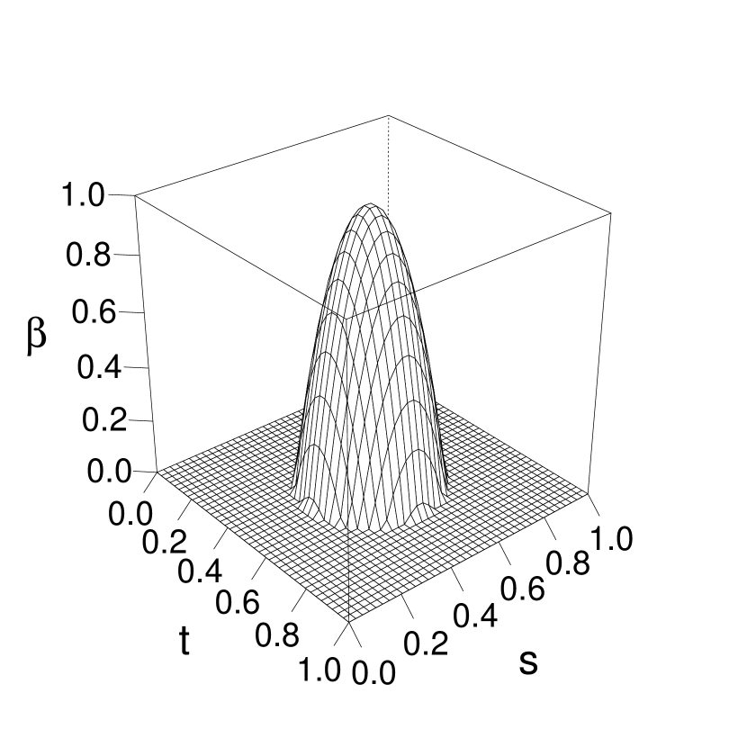
(a)

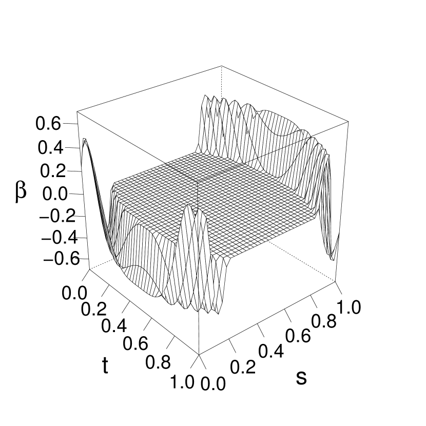
(b)

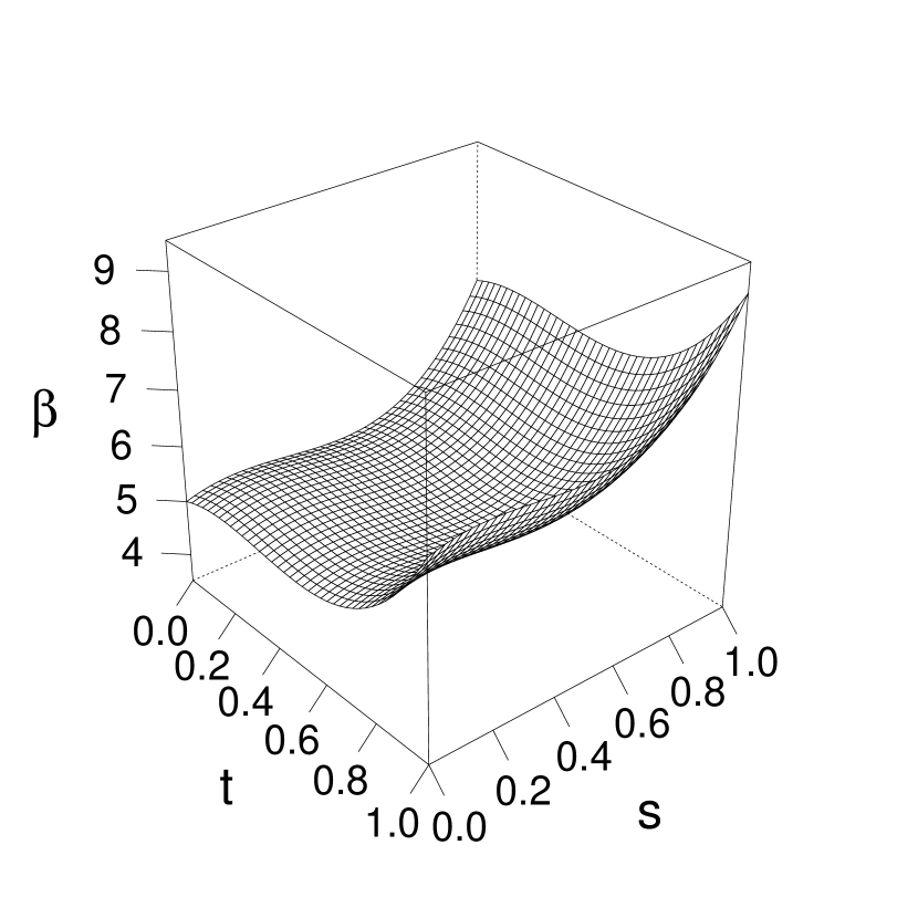
(c)

Figure 2: True coefficient function $\beta$ for Scenario II 2(a), Scenario III 2(b) and Scenario IV 2(c) in the simulation study.

For each scenario, we generate 100 datasets composed of a training set with sample size $n$ and a test set $T$ with size $N$ equal to 4000 that are used to estimate the coefficient function and to test its predictive performance. This is repeated for three different sample sizes $n=150,500,1000$. As in Lin et al. [2017], we consider the integrated squared error (ISE) to asses the quality of the estimator $\hat{\beta}$ of the coefficient function $\beta$. In particular, the ISE over the null region (ISE₀) and the non-null region (ISE₁) are defined as

$$\text{ISE\textsubscript{0}}=\frac{1}{A_{0}}\int\int_{N\left(\beta\right)}\left(\hat{\beta}\left(s,t\right)-\beta\left(s,t\right)\right)^{2}dsdt,\quad\text{ISE\textsubscript{1}}=\frac{1}{A_{1}}\int\int_{NN\left(\beta\right)}\left(\hat{\beta}\left(s,t\right)-\beta\left(s,t\right)\right)^{2}dsdt,$$ (19)

where $A_{0}$ and $A_{1}$ are the measures of the null ($N\left(\beta\right)$) and non-null ($NN\left(\beta\right)$) regions, respectively. The ISE₀ and the ISE₁ are indicators of the estimation error of $\hat{\beta}$ over both the null and the non-null regions. Moreover, predictive performance is measured through the prediction mean squared error (PMSE), defined as

$$\text{PMSE}=\frac{1}{N}\sum_{\left(X,Y\right)\in T}\int_{0}^{1}\left(Y\left(t\right)-\int_{0}^{1}X\left(s\right)\hat{\beta}\left(s,t\right)ds\right)^{2}dt,$$ (20)

where $\hat{\beta}$ is obtained through the observations in the training set. The observations in the test set are centred by means of the sample mean functions estimated through the training set observations.

As a remark, the coefficient function $\beta$ is not identifiable in $L^{2}(\mathcal{S}\times\mathcal{T})$, because the $X_{i}$ is generated as a finite linear combination of basis functions, i.e., not empty null space of $K_{X}$. Thus, as stated in Section 3, $\beta$ is identifiable in the closure of $Im(K_{x})$. To obtain a meaningful measure of the estimation accuracy, both $ISE_{0}$ and $ISE_{1}$ should be computed by considering estimate projections onto $Im(K_{x})$. This means, the methods are compared by considering their estimation performance over the identifiable part of the model, only. However, according to the works of James et al. [2009], Zhou et al. [2013], Lin et al. [2017], the space spanned by the 32 cubic B-splines used to generate $X_{i}$ is sufficiently rich to well approximate both $\beta$ and $\hat{\beta}$ for the proposed and competing methods. Therefore, $ISE_{0}$ and $ISE_{1}$ in Equation (20) can be suitably used to assess the estimation error of the coefficient function over $N\left(\beta\right)$ and $NN\left(\beta\right)$, respectively.

The S-LASSO estimator is compared with four different estimators of $\beta$ which are already present in the literature of the FoF linear regression model estimation. The first two are those proposed by Ramsay and Silverman [2005], where the coefficient function estimator is assumed to be in a finite dimension tensor space with regularization achieved either by choosing the dimension of the tensor space or by introducing roughness penalties. They will be referred to as TRU and SMOOTH estimators, respectively. The third one is the estimator proposed by Ivanescu et al. [2015], Scheipl et al. [2015] (referred to as PFFR), which is implemented in the pffr function of the R package refund. The fourth and fifth ones are those proposed by Yao et al. [2005b], based on the functional principal components analysis (referred to as PCA), and by Canale and Vantini [2016], based on a ridge-type penalization (referred to as RIDGE). The TRU, SMOOTH and S-LASSO are computed by using cubic B-splines with evenly space knot sequences. The dimensions of the B-spline sets that generate the tensor product space for the SMOOTH and S-LASSO estimator are both set equal to 60. Additional results for different choices of the dimensions of the B-spline sets, as well as computational times, are provided in the Supplementary Material D. The tuning parameters of the TRU, SMOOTH, PCA, and RIDGE estimators are chosen by means of $10$-fold cross-validation, viz., the dimension of the tensor basis space for the TRU, the roughness penalties for the SMOOTH, the numbers of retained principal components for the PCA, the penalization parameter for the RIDGE and $\lambda_{s}$, $\lambda_{t}$ and $\lambda_{L}$ for the S-LASSO. In particular the $10$-fold cross-validation for the S-LASSO method is applied with the $0.5$-standard deviation rule. Finally, the PFFR estimator is computed through tensor products of cubic B-splines with 15 basis functions and second-order difference penalties in both directions with smoothing parameters estimated using restricted maximum likelihood (REML).

The performance of the estimators in terms of ISE₀ is displayed in Figure 3. It is not surprising that the estimation error of $\beta$ over $N\left(\beta\right)$ of the S-LASSO estimator is significantly smaller than those of the other estimators, being the capability of recovering sparseness of $\beta$ its main feature. In Scenario I, the RIDGE estimator is the only one that performs comparably to the S-LASSO estimator. This is in accordance with the multivariate setting where it is well known that, when the response is independent of the covariates, the ridge estimator is able to shrink all the coefficients towards zero. The TRU, SMOOTH, PFFR, and PCA estimators have difficulties to correctly identify $N\left(\beta\right)$ for all sample sizes. Nevertheless, their performance is very poor at $n=150$. In Scenario II, the S-LASSO estimator is still the best one to estimate $\beta$ over $N\left(\beta\right)$. However, in this case, the RIDGE estimator performance is unsatisfactory and is mainly caused by the lack of smoothness control that makes the estimator over-rough, especially at small $n$. Among the competitor estimators, the SMOOTH one has the best performance, readily followed by the PFFR estimator. In Scenario III, results are similar to those of Scenario II, even if the TRU estimator appears as the best alternative. Both PCA and RIDGE estimators are not able to successfully recover sparseness of $\beta$ for $n=150$. For the former, the cause is the number of observations not sufficient to capture the covariance structure of the data, whereas for the latter, it is due to the excessive roughness of the estimator. For $n=500$ and $m=1000$, the PFFR estimator performs very poorly. This is due to the incapacity of the REML approach to appropriately select the smoothing parameters.

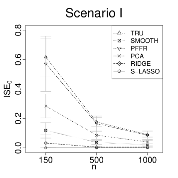
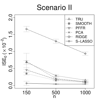
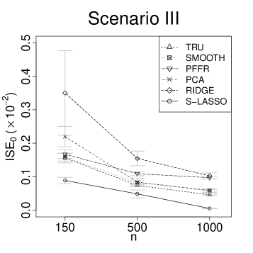
Figure 3: The integrated squared error on the null region (ISE₀) along with $\pm 0.5(standard\hskip 3.41418pterror)$ for the TRU, SMOOTH, PFFR, PCA, RIDGE, and S-LASSO estimators.

Results in terms of ISE₁ are summarized in Figure 4. It is worth noting that, in this case, as expected the performance of the S-LASSO estimator is generally worse than that of the SMOOTH estimator. In some cases, it is worse than that of the TRU and PFFR estimators as well.

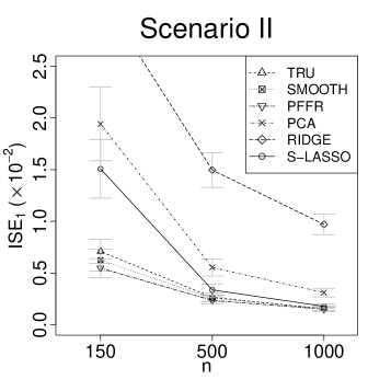
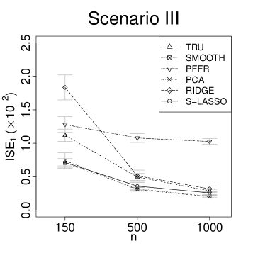
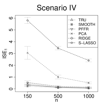
Figure 4: The integrated squared error on the non-null region (ISE₁) along with $\pm 0.5(standard\hskip 3.41418pterror)$ for the TRU, SMOOTH, PFFR, PCA, RIDGE, and S-LASSO estimators.

However, in Scenario II performance differences between the S-LASSO estimator and TRU, SMOOTH or PFFR estimators become negligible as sample size increases. The PCA and RIDGE estimators are always less efficient. The results are similar for Scenario III, where the performance of the S-LASSO estimator is comparable with that of the SMOOTH estimator. Except for the PFFR estimators that badly performs due the difficulties of the REML approach to select the appropriate smoothing parameters, by comparing to the classical LASSO method, the behaviour of the S-LASSO estimator — in terms of ISE₁ — is not surprising. Indeed, it is well known that LASSO method does nice variable selection, even if it tends to overshrink the estimators of the non-null coefficients [Fan et al., 2004, James and Radchenko, 2009]. By looking at the result for Scenario II and III, we surmise that this phenomenon arises in the FoF linear regression model as well. Finally, in Scenario IV, where $\beta$ is always different from zero, the S-LASSO estimator,performs comparably to the SMOOTH (i.e., the S-LASSO estimator with $\lambda_{L}=0$). In this case $\beta$ is not sparse and, thus, the FLP does not help.

Figure 5 shows PMSE averages and corresponding standard errors for all the considered estimators.

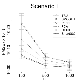
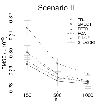
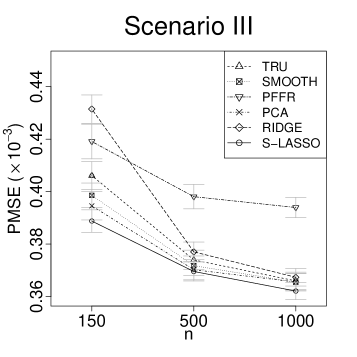
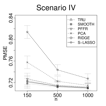
Figure 5: The prediction mean squared error (PMSE) along with $\pm 0.5(standard\hskip 3.41418pterror)$ for the TRU, SMOOTH, PFFR, PCA, RIDGE, and S-LASSO estimators.

Since PMSE is strictly related to the ISE₀ and the ISE₁, results are totally consistent with those of Figure 3 and Figure 4. In particular, the S-LASSO estimator outperforms all the competitor ones in favorable scenarios (viz., Scenario I, II, and III), being the corresponding PMSE lower than that achieved by the other competing estimators. In these scenarios, although the performance of the S-LASSO estimator in terms of ISE₁ is not excellent, the clear superiority in terms of ISE₀ compensates and gives rise to smaller PMSE. Otherwise, for Scenario IV, where the coefficient function is not sparse, the performance of the S-LASSO estimator is very similar to that of the SMOOTH estimator, which is the best one in this case. This is encouraging, because, it proves that the performance of the S-LASSO estimator does not dramatically decline in less favourable scenarios.

In summary, the S-LASSO estimator outperforms the competitors both in terms of estimation error on the null region and prediction accuracy on a new dataset, as well as that it is able to estimate competitively the coefficient function on the non-null region. On the other hand, in order to achieve sparseness, the S-LASSO tends to overshrink the estimator of the coefficient function on the non-null region. This means that, as in the classical setting [James and Radchenko, 2009], there is a trade-off between the ability of recovering sparseness and the estimation accuracy on the non-null region of the final estimator. Moreover, even when the coefficient function is not sparse (Scenario IV), the proposed estimator demonstrates to have both good prediction and estimation performance. This is another key property of the proposed estimator that, encourages practitioners to use the S-LASSO estimator even when there is not prior knowledge about the shape of the coefficient function. Finally, it should be noticed that, in scenarios similar to those analysed, the PCA and RIDGE estimators should not be preferred with respect to the TRU, SMOOTH and S-LASSO ones, and that the PFFR performance is strictly related to the REML approach to select the smoothing parameters.

5 Real-Data Examples

In this section, we analyse two real-data examples. We aim to confirm that the S-LASSO estimator has advantages in terms of both prediction accuracy and interpretability, over the SMOOTH estimator, which has been demonstrated in Section 4 to be the best alternative among the competitors. The datasets used in the examples are the Canadian weather and Swedish mortality. Both are classical benchmark functional data sets thoroughly studied in the literature.

5.1 Canadian Weather Data

The Canadian weather data have been studied by Ramsay and Silverman [2005] and Sun et al. [2018]. The data set contains the daily mean temperature curves, measured in Celsius degree, and the log-scale of the daily rainfall profiles, measured in millimeter, recorded at 35 cities in Canada. Both temperature and rainfall profiles are obtained by averaging over the years 1960 through 1994. Figure 6 shows the profiles.

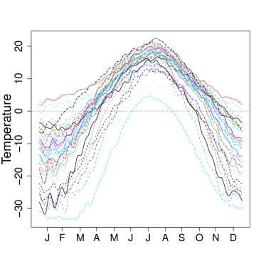
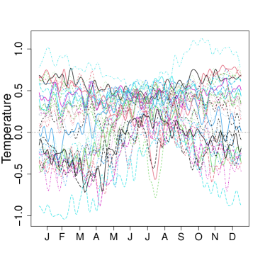
Figure 6: Daily mean temperature and log-daily rainfall profiles at 35 cities in Canada over the year.

The aim is to predict the log-daily rainfall based on the daily temperature using the model reported in Equation (1). Figure 7 shows the S-LASSO and SMOOTH estimates of the coefficient function $\beta$.

Figure 7: S-LASSO ( ) and SMOOTH ([0.5ex][x]0.7cm1pt0.6mm) estimates of the coefficient functions $\beta$ at different months for the Canadian weather data.

The SMOOTH estimate is obtained using a Fourier basis—to take into account the periodicity of the data—and roughness penalties were chosen by using 10-fold cross-validation over an opportune grid of values. 10-fold cross-validation is used to set the parameters $\lambda_{s}$, $\lambda_{t}$ and $\lambda_{L}$ as well.

The S-LASSO estimates is roughly zero over large domain portions. In particular, except for values from July through August, it is always zero in summer months (i.e., late June, July, August and September) and in January and February. This suggests in those months rainfalls are not significantly influenced by daily temperature throughout the year. Otherwise, temperature in fall months (i.e., October, November and December) gives strong positive contribution on the daily rainfalls. In other words, the higher (the lower) the temperature in October, November and December, the heavier (the lighter) the precipitations throughout the year. It is interesting that the S-LASSO estimate in spring months (i.e., March, April and May) is negative for values of $t$ form January through April, and from October through December. This suggests that the higher (the lower) the temperature in the spring the lighter (the heavier) the daily rainfalls from October through April. Finally, it is evidenced a small influence of the temperature in February on precipitations in July and August. It is worth noting that the S-LASSO estimate is more interpretable than the SMOOTH estimates, which does not allow for a straightforward interpretation. Moreover, the S-LASSO estimate appears to have, even if slightly, better prediction performance than the SMOOTH one. Indeed, 10-fold cross-validation mean squared errors are 22.314 and 22.365, respectively.

Finally, we perform two permutation tests to asses the statistical significance of the S-LASSO estimator. The first test is based on the global functional coefficient of determination defined as $R^{2}_{g}\doteq\int_{\mathcal{T}}\frac{\operatorname{Var}\left[\operatorname{E}\left(Y\left(t\right)|X\right)\right]}{\operatorname{Var}\left[Y\left(t\right)\right]}dt$ [Horváth and Kokoszka, 2012], with $\mathcal{T}=\left[0,365\right]$. In Figure 8(a) the solid black line indicates the observed $R^{2}_{g}$ that is equal to 0.55. The bold points represent 500 $R^{2}_{g}$ values obtained by means of random permutations of the response variable. Whereas, the grey line correspond to the $95$th sample percentile.

(a)

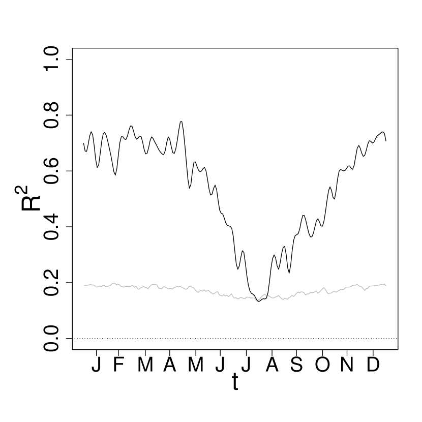
(b)

Figure 8: For the Canadian weather data, 8(a) $R^{2}_{g}$ from permuting the response 500 times, where the black line corresponds to the observed $R^{2}_{g}$ and the grey line to the $95$th sample percentile; 8(b) the black line is the observed $R^{2}$ and the grey line is the pointwise $95$th sample percentile curve.

All 100 values of $R^{2}$ as well as the value of the $95$th sample percentile is far below 0.55, which gives a strong evidence of a significant relationship between rainfalls and temperature, globally.
By a second test, we aim to analyse the pointwise statistical significance, i.e., for each $t\in\mathcal{T}$. It is based on the pointwise functional coefficient of determination defined as $R^{2}\left(t\right)\doteq\frac{\operatorname{Var}\left[\operatorname{E}\left(Y\left(t\right)|X\right)\right]}{\operatorname{Var}\left[Y\left(t\right)\right]}$ for $t\in\mathcal{T}$ [Horváth and Kokoszka, 2012]. Figure 8(b) shows the observed $R^{2}$ (solid black line) along with the pointwise $95$th sample percentile curve. The latter has been obtained by means of 500 $R^{2}$ values produced by randomly permuting the response variable. The observed $R^{2}$ is far above the $95$th sample percentile curve, except for some summer months (viz., July and August). As global conclusion, we can state that the temperature has a large influence on the rainfalls in autumn, winter and spring.

5.2 Swedish Mortality Data

The Swedish mortality data, available from the Human Mortality Database (http://mortality.org), are regarded as a very reliable dataset on long-term longitudinal mortalities. In particular, we focus on the log-hazard rate functions of the Swedish females mortality data for year-of-birth cohorts that refer to females born in the years 1751-1894 with ages 0-80. The value of a log-hazard rate function at a given age is the natural logarithm of the ratio of the number of females who died at that age and the number of females alive with the same age. Note that, those data have been analysed also by Chiou and Müller [2009] and Ramsay et al. [2009]. Figure 9 shows the 144 log-hazard functions.

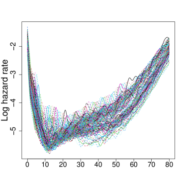
Figure 9: Log-hazard rates as a function of age for Swedish female cohorts born in the years 1751-1894.

The aim of the analysis is to explore the relationship of the log-hazard rate function for a given year with the log-hazard rate curve of the previous year by means of the model reported in Equation (1). Our interest is to identify what features of the log-hazard rate functions for a given year influence the log-hazard rate of the following year.

Figure 10 shows the S-LASSO and SMOOTH estimates of coefficient function $\beta$.

Figure 10: S-LASSO ( ) and SMOOTH ([0.5ex][x]0.7cm1pt0.6mm) estimates of the coefficient functions $\beta$ at different values of $t$ for the Swedish mortality data.

The unknown parameters to obtain the SMOOTH and S-LASSO estimates are chosen as in the Canadian weather example, but in this case B-splines are used for both estimators. The S-LASSO estimate is zero almost over all the domain except for few regions. In particular, at given $t$, the S-LASSO estimate is different from zero in an interval located right after that age. This can likely support the conjecture that if an event influences the mortality of the Swedish female at a given age, it impacts on the the death rate below that age born in the following years. Nevertheless, this expected dependence is poorly pointed out by the SMOOTH estimator, where this behaviour is confounded by less meaningful periodic components. It is interesting to note that the S-LASSO estimate at high values of $t$ is slightly different from zero for ages ranging from 40 to 60. This shows that if an event affecting the death rate occurs in that range, the log-hazard functions of the following cohorts will be influenced at high ages (i.e., corresponding to high values of $t$). On the contrary, the wiggle of the SMOOTH estimate does not allow drawing such conclusions.

Finally, we perform the two permutation tests already described in the Canadian weather data example. Figure 11 shows the results. Both the observed $R^{2}_{g}$ and $R^{2}$ are far above the $95$th sample percentile (Figure 11(a)) and the pointwise $95$th sample percentile curve (Figure 11(b)) respectively. This significantly evidences a relation between two consecutive log-hazard rate functions for all ages.

(a)

(b)

Figure 11: For the Swedish mortality data, 8(a) $R^{2}_{g}$ from permuting the response 500 times, where the black line corresponds to the observed $R^{2}_{g}$ and the grey line to the $95$th sample percentile; 8(b) the black line is the observed $R^{2}$ and the grey line is the pointwise $95$th sample percentile curve.

5.3 Ship CO₂ Emission Data

The ship CO₂ emission data have been previously studied in [Lepore et al., 2018, Reis et al., 2019, Capezza et al., 2020, Centofanti et al., 2020b, a]. The dataset, provided by the shipping company Grimaldi Group, regards the issue of monitoring fuel consumptions or CO₂ emissions for a Ro-Pax ship that sails along a route in the Mediterranean Sea. The aim of the analysis is to study the relation between the fuel consumption per hour (FCPH), which is a proxy of the CO₂ emissions, and the speed over ground (SOG), assumed as predictor. The observations considered were recorded from 2015 to 2017. Figure 12 shows the 44 available observations of SOG and FCPH [Centofanti et al., 2020b].

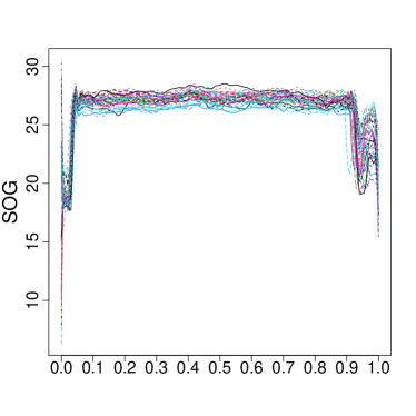
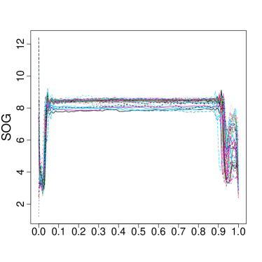
Figure 12: SOG and FCPH observations from a Ro-Pax ship.

Then, Figure 13 displays the S-LASSO and SMOOTH estimates of coefficient function $\beta$ estimated as described in the Swedish mortality example.

Figure 13: S-LASSO ( ) and SMOOTH ([0.5ex][x]0.7cm1pt0.6mm) estimates of the coefficient functions $\beta$ at different values of $t$ for the ship CO₂ emission data.

The S-LASSO coefficient function estimate also in this example is different from zero over a small portion of domain. Specifically, the FCPH during the navigation phase (i.e., $t\in\left[0.1,0.9\right]$) is positively influenced by the SOG, in three specific voyage instants, viz., $s\approx 0.15,0.55,0.85$, where the coefficient function estimate is positive. Thus, the FCPH during the navigation phase positively depends on the SOG at the start, in the middle and at the end of the navigation phase. Differently, during acceleration ($t\in\left[0,0.1\right]$) and deceleration ($t\in\left[0.9,1\right]$) phases, the relationship between the FCPH and the SOG is mainly concurrent. That is, the FCPH observed at a given time instant is strictly related to the SOG observed at the same time. On the contrary, such interpretation of the FCPH-SOG relationship is not easily obtained through the analysis of the SMOOTH coefficient function estimate, which is overall different from zero. Moreover, the S-LASSO and the SMOOTH estimates achieve 10-fold cross-validation mean squared errors of 0.077 and 0.093, respectively. Thus, the proposed estimator achieves slightly better prediction performance than the competitor.

Figure 14 shows the results for the two permutation tests already described in the Canadian weather and Swedish mortality data examples. The relation between the FCPH and the SOG can be then considered as significant, as both the observed $R^{2}_{g}$ and $R^{2}$ are above the $95$th sample percentile (Figure 14(a)) and the pointwise $95$th sample percentile curve (Figure 14(b)), respectively.

(a)

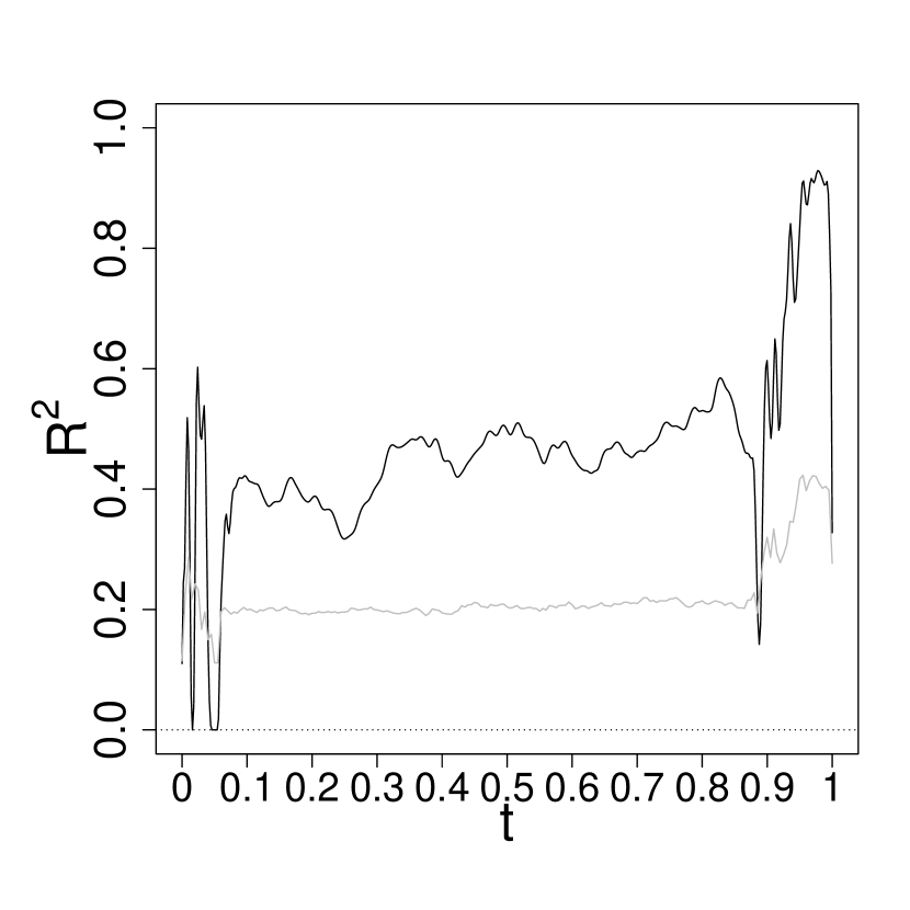
(b)

Figure 14: For the ship CO₂ data, 14(a) $R^{2}_{g}$ from permuting the response 500 times, where the black line corresponds to the observed $R^{2}_{g}$ and the grey line to the $95$th sample percentile; 14(b) the black line is the observed $R^{2}$ and the grey line is the pointwise $95$th sample percentile curve.

6 Conclusion

The LASSO is one of the most used and popular method to estimate coefficients in classical linear regression models as it ensures both prediction accuracy and interpretability of the phenomenon under study (by simultaneously performing variable selection). In this paper, we propose the S-LASSO estimator for the coefficient function of the Function-on-Function (FoF) linear regression model, which is an extension to the functional setting of the multivariate LASSO estimator. As the latter, the S-LASSO estimator is able to increase both the prediction accuracy of the estimated model, via continuous shrinking, and the interpretability, by identifying the null region of the regression coefficient, i.e., the region where the coefficient function is exactly zero.

The S-LASSO estimator is obtained by combining several elements: the functional LASSO penalty (FLP), which has the task of shrinking towards zero the estimator on the null region; the B-splines, which are essential to ensure sparsity of the estimator because of the compact support property; and two roughness penalties, which are needed to ensure smoothness of the estimator on the non-null region, also when the number of B-splines escalates. We proved that the S-LASSO estimator is both estimation and point-wise sign consistent, i.e., the estimation error in terms of $L^{2}$-norm goes to zero in probability and the S-LASSO estimator has the same sign of the true coefficient function with probability tending to one. Moreover, we showed via an extensive Monte Carlo simulation study that, with respect to other methods that have already appeared in the literature, the S-LASSO estimator is much more interpretable, on the one hand, and has still good estimation and appealing predictive performance, on the other. However, consistently with the behaviour of the classical LASSO estimator [Fan et al., 2004], the S-LASSO estimator is found sometimes to over-shrink the coefficient function over the non-null region.

Note that the S-LASSO method is in the spirit of the fused LASSO of Tibshirani et al. [2005] in the multivariate context. Both methods rely on penalties that encourage sparsity in the coefficients and impose smoothness in the coefficient profile. The smoothness penalties of the proposed S-LASSO estimator and the fused LASSO approach have a different nature. In the fused LASSO, the differences of two consecutive coefficients are in fact penalized in their absolute value thus shrinking consecutive coefficients to the same value. On the contrary, the S-LASSO estimator relies on quadratic smoothness penalties that do not enjoy the sparseness property. Moreover, while the fused LASSO considers penalization of the first differences, the S-LASSO estimator allows the penalization of several types of smoothness, through the $m$s-th and $m$t-th order linear differential operators applied to the coefficient function.

To the best of the authors knowledge, this is the first work that addresses the issue of interpretability, intended as sparseness of the coefficient function, in the FoF linear regression setting. However, although the FLP produces an estimator with good properties, other penalties, e.g. the SCAD [Fan and Li, 2001] and adaptive LASSO [Zou, 2006], properly adapted to the functional setting, may guarantee even better performance both in terms of interpretabilty and prediction accuracy, and are, indeed, subjects of ongoing research.

References

- Abramowicz et al. [2018] Abramowicz K, Häger CK, Pini A, Schelin L, Sjöstedt de Luna S, Vantini S. Nonparametric inference for functional-on-scalar linear models applied to knee kinematic hop data after injury of the anterior cruciate ligament. Scandinavian Journal of Statistics 2018;45(4):1036–61.
- Andrew and Gao [2007] Andrew G, Gao J. Scalable training of l 1-regularized log-linear models. In: Proceedings of the 24th international conference on Machine learning. ACM; 2007. p. 33–40.
- Besse and Cardot [1996] Besse PC, Cardot H. Approximation spline de la prévision d’un processus fonctionnel autorégressif d’ordre 1. Canadian Journal of Statistics 1996;24(4):467–87.
- Bosq [2000] Bosq D. Linear processes in function spaces: theory and applications. volume 149. Springer Science & Business Media, 2000.
- Canale and Vantini [2016] Canale A, Vantini S. Constrained functional time series: Applications to the italian gas market. International Journal of Forecasting 2016;32(4):1340–51.
- Candes et al. [2007] Candes E, Tao T, et al. The dantzig selector: Statistical estimation when p is much larger than n. The Annals of Statistics 2007;35(6):2313–51.
- Capezza et al. [2020] Capezza C, Lepore A, Menafoglio A, Palumbo B, Vantini S. Control charts for monitoring ship operating conditions and CO2 emissions based on scalar-on-function regression. Applied Stochastic Models in Business and Industry 2020;.
- Cardot et al. [2003] Cardot H, Ferraty F, Sarda P. Spline estimators for the functional linear model. Statistica Sinica 2003;:571–91.
- Centofanti et al. [2020a] Centofanti F, Lepore A, Menafoglio A, Palumbo B, Vantini S. Adaptive smoothing spline estimator for the function-on-function linear regression model. arXiv preprint arXiv:201112036 2020a;.
- Centofanti et al. [2020b] Centofanti F, Lepore A, Menafoglio A, Palumbo B, Vantini S. Functional regression control chart. Technometrics 2020b;:1–14.
- Chiou et al. [2014] Chiou JM, Chen YT, Yang YF. Multivariate functional principal component analysis: A normalization approach. Statistica Sinica 2014;:1571–96.
- Chiou and Müller [2009] Chiou JM, Müller HG. Modeling hazard rates as functional data for the analysis of cohort lifetables and mortality forecasting. Journal of the American Statistical Association 2009;104(486):572–85.
- Cuevas [2014] Cuevas A. A partial overview of the theory of statistics with functional data. Journal of Statistical Planning and Inference 2014;147:1–23.
- De Boor [2001] De Boor C. A practical guide to splines. Springer-verlag New York, 2001.
- Efron et al. [2004] Efron B, Hastie T, Johnstone I, Tibshirani R, et al. Least angle regression. The Annals of statistics 2004;32(2):407–99.
- Fan and Li [2001] Fan J, Li R. Variable selection via nonconcave penalized likelihood and its oracle properties. Journal of the American statistical Association 2001;96(456):1348–60.
- Fan et al. [2004] Fan J, Peng H, et al. Nonconcave penalized likelihood with a diverging number of parameters. The Annals of Statistics 2004;32(3):928–61.
- Friedman et al. [2010] Friedman J, Hastie T, Tibshirani R. Regularization paths for generalized linear models via coordinate descent. Journal of statistical software 2010;33(1):1.
- Hall et al. [2007] Hall P, Horowitz JL, et al. Methodology and convergence rates for functional linear regression. The Annals of Statistics 2007;35(1):70–91.
- Hastie et al. [2009] Hastie T, Tibshirani R, Friedman J. The elements of statistical learning: data mining, inference, and prediction. Springer series in statistics New York, NY, USA:, 2009.
- Horváth and Kokoszka [2012] Horváth L, Kokoszka P. Inference for functional data with applications. volume 200. Springer Science & Business Media, 2012.
- Hsing and Eubank [2015] Hsing T, Eubank R. Theoretical foundations of functional data analysis, with an introduction to linear operators. John Wiley & Sons, 2015.
- Ivanescu et al. [2015] Ivanescu AE, Staicu AM, Scheipl F, Greven S. Penalized function-on-function regression. Computational Statistics 2015;30(2):539–68.
- James and Radchenko [2009] James GM, Radchenko P. A generalized dantzig selector with shrinkage tuning. Biometrika 2009;96(2):323–37.
- James et al. [2009] James GM, Wang J, Zhu J, et al. Functional linear regression that’s interpretable. The Annals of Statistics 2009;37(5A):2083–108.
- Jia and Yu [2010] Jia J, Yu B. On model selection consistency of the elastic net when p n. Statistica Sinica 2010;:595–611.
- Kokoszka and Reimherr [2017] Kokoszka P, Reimherr M. Introduction to functional data analysis. CRC Press, 2017.
- Lepore et al. [2018] Lepore A, Palumbo B, Capezza C. Analysis of profiles for monitoring of modern ship performance via partial least squares methods. Quality and Reliability Engineering International 2018;34(7):1424–36.
- Li et al. [2007] Li Y, Hsing T, et al. On rates of convergence in functional linear regression. Journal of Multivariate Analysis 2007;98(9):1782–804.
- Lin et al. [2017] Lin Z, Cao J, Wang L, Wang H. Locally sparse estimator for functional linear regression models. Journal of Computational and Graphical Statistics 2017;26(2):306–18.
- Morris [2015] Morris JS. Functional regression. Annual Review of Statistics and Its Application 2015;2:321–59.
- Nocedal and Wright [2006] Nocedal J, Wright S. Numerical optimization. Springer Science & Business Media, 2006.
- Prchal and Sarda [2007] Prchal L, Sarda P. Spline estimator for the functional linear regression with functional response. Preprint 2007;.
- Ramsay and Silverman [2005] Ramsay J, Silverman B. Functional Data Analysis. Springer Series in Statistics. Springer, 2005.
- Ramsay et al. [2009] Ramsay JO, Hooker G, Graves S. Functional data analysis with R and MATLAB. Springer Science & Business Media, 2009.
- Reis et al. [2019] Reis MS, Rendall R, Palumbo B, Lepore A, Capezza C. Predicting ships’ CO2 emissions using feature-oriented methods. Applied Stochastic Models in Business and Industry 2019;.
- Scheipl and Greven [2016] Scheipl F, Greven S. Identifiability in penalized function-on-function regression models. Electronic Journal of Statistics 2016;10(1):495–526.
- Scheipl et al. [2015] Scheipl F, Staicu AM, Greven S. Functional additive mixed models. Journal of Computational and Graphical Statistics 2015;24(2):477–501.
- Schumaker [2007] Schumaker L. Spline functions: basic theory. Cambridge University Press, 2007.
- Sun et al. [2018] Sun X, Du P, Wang X, Ma P. Optimal penalized function-on-function regression under a reproducing kernel hilbert space framework. Journal of the American Statistical Association 2018;:1–11.
- Tibshirani [1996] Tibshirani R. Regression shrinkage and selection via the lasso. Journal of the Royal Statistical Society Series B (Methodological) 1996;:267–88.
- Tibshirani et al. [2005] Tibshirani R, Saunders M, Rosset S, Zhu J, Knight K. Sparsity and smoothness via the fused lasso. Journal of the Royal Statistical Society: Series B (Statistical Methodology) 2005;67(1):91–108.
- Yao et al. [2005a] Yao F, Müller HG, Wang JL. Functional data analysis for sparse longitudinal data. Journal of the American Statistical Association 2005a;100(470):577–90.
- Yao et al. [2005b] Yao F, Müller HG, Wang JL. Functional linear regression analysis for longitudinal data. The Annals of Statistics 2005b;:2873–903.
- Zhou and Chen [2012] Zhou J, Chen M. Spline estimators for semi-functional linear model. Statistics & Probability Letters 2012;82(3):505–13.
- Zhou et al. [2013] Zhou J, Wang NY, Wang N. Functional linear model with zero-value coefficient function at sub-regions. Statistica Sinica 2013;23(1):25.
- Zou [2006] Zou H. The adaptive lasso and its oracle properties. Journal of the American statistical association 2006;101(476):1418–29.
- Zou and Zhang [2009] Zou H, Zhang HH. On the adaptive elastic-net with a diverging number of parameters. Annals of statistics 2009;37(4):1733.