Cluster–galaxy weak lensing

Abstract

Weak gravitational lensing of background galaxies provides a direct probe of the projected matter distribution in and around galaxy clusters. Here we present a self-contained pedagogical review of cluster–galaxy weak lensing, covering a range of topics relevant to its cosmological and astrophysical applications. We begin by reviewing the theoretical foundations of gravitational lensing from first principles, with special attention to the basics and advanced techniques of weak gravitational lensing. We summarize and discuss key findings from recent cluster–galaxy weak-lensing studies on both observational and theoretical grounds, with a focus on cluster mass profiles, the concentration–mass relation, the splashback radius, and implications from extensive mass calibration efforts for cluster cosmology.

1 Introduction

The propagation of light rays from a distant source to the observer is governed by the gravitational field of local inhomogeneities, as well as by the global geometry of the universe (Schneider et al., 1992). Hence the images of background sources carry the imprint of gravitational lensing by intervening cosmic structures. Observations of gravitational lensing phenomena can thus be used to study the mass distribution of cosmic objects dominated by dark matter and to test models of cosmic structure formation (Blandford and Narayan, 1992).

Galaxy clusters represent the largest class of self-gravitating systems formed in the universe, with typical masses of $M\sim 10^{14-15}h^{-1}M_{\odot}$. In the context of the standard structure formation scenario, cluster halos correspond to rare massive local peaks in the primordial density perturbations (e.g., Tinker et al., 2010). Galaxy clusters act as powerful cosmic lenses, producing a variety of detectable lensing effects from strong to weak lensing (Kneib and Natarajan, 2011), including deflection, shearing, and magnifying of the images of background sources (e.g., Umetsu et al., 2016). The critical advantage of cluster gravitational lensing is its ability to study the mass distribution of individual and ensemble systems independent of assumptions about their physical and dynamical state (e.g., Clowe et al., 2006).

Weak gravitational lensing is responsible for the weak shape distortion, or shear, and magnification of the images of background sources due to the gravitational field of intervening massive objects and large scale structure (Bartelmann et al., 2001; Schneider, 2005; Umetsu, 2010; Hoekstra, 2013; Mandelbaum, 2018). Weak shear lensing by galaxy clusters gives rise to levels of up to a few 10 percent of elliptical distortions in images of background sources. Thus, the weak shear lensing signal, as measured from small but coherent image distortions in galaxy shapes, can provide a direct measure of the projected mass distribution of galaxy clusters (e.g., Kaiser and Squires, 1993; Fahlman et al., 1994; Okabe and Umetsu, 2008). On the other hand, lensing magnification can influence the observed surface number density of background galaxies seen behind clusters, by enhancing their apparent fluxes and expanding the area of sky (e.g., Broadhurst et al., 1995, 2005b; Taylor et al., 1998; Umetsu et al., 2011b; Chiu et al., 2020). The former effect increases the source counts above the limiting flux, whereas the latter reduces the effective observing area in the source plane, thus decreasing the observed number of sources per unit solid angle. The net effect, known as magnification bias, depends on the intrinsic faint-end slope of the source luminosity function.

In this paper, we present a self-contained pedagogical review of weak gravitational lensing of background galaxies by galaxy clusters (cluster–galaxy weak lensing), highlighting recent advances in our theoretical and observational understanding of the mass distribution in galaxy clusters. We shall begin by reviewing the theoretical foundations of gravitational lensing (Sect. 2), with special attention to the basics and advanced techniques of cluster–galaxy weak lensing (Sects. 3, 4, and 5). Then, we highlight and discuss key findings from recent cluster–galaxy weak-lensing studies (Sects. 6), with a focus on cluster mass distributions (Sect. 6.1), the concentration–mass relation (Sect. 6.2), the splashback radius (Sect. 6.3), and implications from extensive mass calibration efforts for cluster cosmology (Sect. 6.4). Finally, conclusions are given in Sect. 7.

There have been a number of reviews of relevant subjects (e.g., Blandford and Narayan, 1992; Narayan and Bartelmann, 1996; Mellier, 1999; Hattori et al., 1999; Umetsu et al., 1999; Van Waerbeke and Mellier, 2003; Schneider, 2005; Kneib and Natarajan, 2011; Hoekstra, 2013; Futamase, 2015; Mandelbaum, 2018). For general treatments of gravitational lensing, we refer the reader to Schneider et al. (1992). For a general review of weak gravitational lensing, see Bartelmann and Schneider (2001) and Schneider (2005). For a comprehensive review of cluster lensing, see Kneib and Natarajan (2011). For a pedagogical review on strong lensing in galaxy clusters, see Hattori et al. (1999).

Throughout this paper, we denote the present-day density parameters of matter, radiation, and $\mathrm{\Lambda}$ (a cosmological constant) in critical units as $\mathrm{\Omega}_{\mathrm{m}},\mathrm{\Omega}_{\mathrm{r}}$, and $\mathrm{\Omega}_{\mathrm{\Lambda}}$, respectively (see, e.g., Komatsu et al., 2009). Unless otherwise noted, we assume a concordance $\mathrm{\Lambda}$ cold dark matter ($\mathrm{\Lambda}$CDM) cosmology with $\mathrm{\Omega}_{\mathrm{m}}=0.3$, $\mathrm{\Omega}_{\mathrm{\Lambda}}=0.7$, and a Hubble constant of $H_{0}=100\,h$ km s^-1 Mpc^-1 with $h=0.7$. We denote the mean matter density of the universe at a particular redshift $z$ as $\overline{\rho}(z)$ and the critical density as $\rho_{\mathrm{c}}(z)$. The present-day value of the critical density is $\rho_{\mathrm{c,0}}=3H_{0}^{2}/(8\pi G)\approx 1.88\times 10^{-29}h^{2}$ g  cm${}^{-3}\approx 2.78\times 10^{11}h^{2}M_{\odot}$ Mpc^-3, with $G$ the gravitational constant. We use the standard notation $M_{\Delta_{\mathrm{c}}}$ or $M_{\Delta_{\mathrm{m}}}$ to denote the mass enclosed within a sphere of radius $r_{\Delta_{\mathrm{c}}}$ or $r_{\Delta_{\mathrm{m}}}$, within which the mean overdensity equals $\Delta_{\mathrm{c}}\times\rho_{\mathrm{c}}(z)$ or $\Delta_{\mathrm{m}}\times\overline{\rho}(z)$ at a particular redshift $z$. That is, $M_{\Delta_{\mathrm{c}}}=(4\pi/3)\Delta_{\mathrm{c}}\rho_{\mathrm{c}}(z)r_{\Delta_{\mathrm{c}}}^{3}$ and $M_{\Delta_{\mathrm{m}}}=(4\pi/3)\Delta_{\mathrm{m}}\overline{\rho}(z)r_{\Delta_{\mathrm{m}}}^{3}$. We generally denote three-dimensional radial distances as $r$ and reserve the symbol $R$ for projected radial distances. Unless otherwise noted, we use projected densities (e.g., $\Sigma(R)$) and distances (e.g., $R$) both defined in physical (not comoving) units. All quoted errors are $1\sigma$ confidence levels (CL) unless otherwise stated.

2 Theory of gravitational lensing

The local universe appears to be highly inhomogeneous on a wide range of scales from stars, galaxies, through galaxy groups and clusters, to forming superclusters, large-scale filaments, and cosmic voids. The propagation of light from a far-background source is thus influenced by the gravitational field caused by such local inhomogeneities along the line of sight. In general, a complete description of the light propagation in an arbitrary curved spacetime is a complex theoretical problem. However, a much simpler description is possible under a wide range of astrophysically relevant circumstances, which is referred to as the gravitational lensing theory (e.g., Schneider et al., 1992; Bartelmann and Schneider, 2001; Kneib and Natarajan, 2011). This section reviews the basics of gravitational lensing theory to provide a basis and framework for cluster lensing studies, with an emphasis on weak gravitational lensing.

2.1 Bending of light in an asymptotically flat spacetime

To begin with, let us consider the bending of light in a weak-field regime of an asymptotically flat spacetime in the framework of general relativity. Specifically, we assume an isolated and stationary mass distribution (Schneider et al., 1992). Then, the metric tensor $g_{\mu\nu}$ ($\mu,\nu=0,1,2,3$) of the perturbed spacetime can be written as:

$$ds^{2} =g_{\mu\nu}dx^{\mu}dx^{\nu}$$ (1)

$$=-(1+2\Phi_{\mathrm{N}}/c^{2})c^{2}dt^{2}+(1-2\Phi_{\mathrm{N}}/c^{2})\left[(dx^{1})^{2}+(dx^{2})^{2}+(dx^{3})^{2}\right],$$

where $(x^{\mu})=(ct,x^{1},x^{2},x^{3})$ are the four spacetime coordinates, $\Phi_{\mathrm{N}}$ is the Newtonian gravitational potential in a weak-field regime $|\Phi_{\mathrm{N}}/c^{2}|\ll 1$, and $c$ is the speed of light in vacuum. We consider the metric given by Eq. (1) to be the sum of a background metric $g_{\mu\nu}^{(\mathrm{b})}$ and a small perturbation denoted by $h_{\mu\nu}$, that is, $g_{\mu\nu}=g_{\mu\nu}^{(\mathrm{b})}+h_{\mu\nu}$ with $|h_{\mu\nu}|\ll 1$.

To the first order in $\Phi_{\mathrm{N}}/c^{2}$, we have $g_{\mu\nu}^{(\mathrm{b})}=\eta_{\mu\nu}=\mathrm{diag}(-1,1,1,1)$ and $h_{\mu\nu}=\mathrm{diag}(-2\Phi_{\mathrm{N}},-2\Phi_{\mathrm{N}},-2\Phi_{\mathrm{N}},-2\Phi_{\mathrm{N}})/c^{2}$, where $g^{\mu\nu}$ and $g^{(\mathrm{b})\mu\nu}$ are defined by $g^{\mu\rho}g_{\rho\nu}=\delta^{\mu}_{\nu}$ and $g^{(\mathrm{b})\mu\rho}g^{(\mathrm{b})}_{\rho\nu}=\delta^{\mu}_{\nu}$, with $\delta^{\mu}_{\nu}$ the Kronecker delta symbol in four dimensions. Then, to the first order of $h$, we have $g^{\mu\nu}=g^{(\mathrm{b})\mu\nu}-h^{\mu\nu}$, where $h^{\mu\nu}$ is defined by $h^{\mu\nu}\equiv g^{(\mathrm{b})\mu\rho}g^{(\mathrm{b})\nu\sigma}h_{\rho\sigma}=\eta^{\mu\rho}\eta^{\nu\sigma}h_{\rho\sigma}$.

The propagation of light is described by null geodesic equations:

$$k^{\mu} \equiv\frac{dx^{\mu}(\lambda)}{d\lambda},$$ (2)

$$0 =g_{\mu\nu}k^{\mu}k^{\nu},$$

$$\frac{dk^{\mu}}{d\lambda} =-\Gamma^{\mu}_{\nu\lambda}k^{\nu}k^{\lambda},$$

where $k^{\mu}$ is the four-momentum, $\lambda$ is the affine parameter, and $\Gamma^{\mu}_{\nu\lambda}$ denotes the Christoffel symbol, $\Gamma^{\mu}_{\nu\rho}=(1/2)g^{\mu\lambda}\left(g_{\lambda\nu,\rho}+g_{\lambda\rho,\nu}-g_{\nu\rho,\lambda}\right)$, with $g_{\mu\nu}^{(\mathrm{b})}=\eta_{\mu\nu}$ and $\Gamma^{(\mathrm{b})\mu}_{\nu\rho}=0$ in the background Minkowski spacetime. For a light ray propagating along the $x^{3}$-direction in the background metric, the photon four-momentum $k^{(\mathrm{b})\mu}$ and the unperturbed orbit $x^{(\mathrm{b})\mu}$ are given by $k^{(\mathrm{b})\mu}=dx^{(\mathrm{b})\mu}/d\lambda=(1,0,0,1)$ and $x^{(\mathrm{b})\mu}=(\lambda,0,0,\lambda)$.

Now we consider the light ray propagation in a perturbed spacetime. To this end, we express the perturbed orbit $x^{\mu}(\lambda)$ as a sum of the unperturbed path $x^{(\mathrm{b})\mu}(\lambda)$ and the deviation vector $\delta x^{\mu}(\lambda)$:

$$x^{\mu}(\lambda)=x^{(\mathrm{b})\mu}(\lambda)+\delta x^{\mu}(\lambda).$$ (3)

Without loss of generality, we can take the deflection angle to lie in the $x^{3}x^{1}$ plane with $x^{2}=0$, and we denote $(x^{1},x^{3})=(x^{\perp},x^{||})$. In the weak-field limit of $|\Phi_{\mathrm{N}}/c^{2}|\ll 1$, the impact parameter $b$ of the incoming light ray is much greater than the Schwarzschild radius of the deflector with mass $M$, that is, $b\gg 2GM/c^{2}$. Then, the linearized null geodesic equations are written as:

$$k^{\mu}(\lambda) =k^{(\mathrm{b})\mu}(\lambda)+\delta k^{\mu}(\lambda),$$ (4)

$$0 =h_{\mu\nu}k^{(\mathrm{b})\mu}k^{(\mathrm{b})\nu}+2g^{(\mathrm{b})}_{\mu\nu}k^{(\mathrm{b})\mu}\delta k^{\nu},$$

$$\frac{d(\delta k^{\mu})}{d\lambda} =-2\Gamma^{(\mathrm{b})\mu}_{\nu\lambda}k^{(\mathrm{b})\nu}\delta k^{\lambda}-\delta\Gamma^{\mu}_{\nu\lambda}k^{(\mathrm{b})\nu}k^{(\mathrm{b})\lambda}.$$

The perturbed Christoffel symbol is $\delta\Gamma^{\mu}_{\nu\rho}=(1/2)\eta^{\mu\lambda}\left(h_{\lambda\nu,\rho}+h_{\lambda\rho,\nu}-h_{\nu\rho,\lambda}\right)+O(h^{2})$. Choosing the boundary conditions in the in-state ($\lambda\to-\infty$) as $\delta k^{\mu}(-\infty)=0$, we integrate the linearized null geodesic equations (Eq. (4)) to obtain the following equations for the spatial components in the out-state ($\lambda\to+\infty$):

$$\delta k^{\perp}(+\infty)=-\frac{2}{c^{2}}\int_{-\infty}^{+\infty}\frac{\partial\Phi_{\mathrm{N}}(\lambda)}{\partial x^{\perp}}\,d\lambda,\ \ \ \delta k^{||}(+\infty)=0,$$ (5)

where $\lambda=x^{||}(\lambda)+O(h)$. Taking the unperturbed path, we obtain the bending angle $\hat{\alpha}$ in the small angle scattering limit ($|\hat{\alpha}|\ll 1$) as:

$$\hat{\alpha}\simeq\frac{k^{\perp}(+\infty)}{k^{||}(+\infty)}\simeq-\frac{2}{c^{2}}\int_{-\infty}^{+\infty}\!\frac{\partial\Phi_{\mathrm{N}}(x^{||},x^{\perp})}{\partial x^{\perp}}\,dx^{||},$$ (6)

which is known as the Born approximation. This yields an explicit expression for the bending angle of $|\hat{\alpha}|\simeq 4GM/(rc^{2})=1.75^{\prime\prime}(M/M_{\odot})(r/R_{\odot})^{-1}$. General relativity predicts a deflection angle twice as large as that Newtonian physics would provide. Einstein’s prediction for the solar deflection of light is verified within $\sim 0.1\%$ (e.g., Lebach et al., 1995).

The null geodesic condition leads to $\delta k^{0}(\lambda)=-2\Phi_{\mathrm{N}}(\lambda)/c^{2}+O(h^{2})$, or $cdt/d\lambda=1-2\Phi_{\mathrm{N}}(\lambda)/c^{2}+O(h^{2})>1$. The gravitational time delay $\Delta t_{\mathrm{grav}}$, with respect to the unperturbed light propagation, is thus given by:

$$c\Delta t_{\mathrm{grav}}=-2\int_{-\infty}^{+\infty}\!d\lambda\,\Phi_{\mathrm{N}}(\lambda)/c^{2}.$$ (7)

Note that there is an additional time delay due to a change in the geometrical path length caused by gravitational deflection (see Sect. 2.6.1).

2.2 Lens equation

Figure 1: Illustration of a typical lens system. The light ray propagates from the source (S) at the position $\eta$ in the source plane to the observer (O), passing the position $\xi$ in the lens plane (L), resulting in a bending angle $\hat{\mbox{\boldmath$\alpha$}}$. The angular position of the source (S) relative to the optical axis is denoted by $\beta$, and that of the image (I) relative to the optical axis is denoted by $\theta$. The $D_{l}$, $D_{s}$, and $D_{ls}$ are the observer–lens, observer–source, and lens–source angular diameter distances, respectively.

Let us consider the situation illustrated in Fig. 1. A light ray propagates from a far-distant source (S) at the position $\eta$ in the source plane to an observer (O), passing the position $\xi$ in the lens plane, in which the light is deflected by a bending angle $\hat{\mbox{\boldmath$\alpha$}}$. Here the source and lens planes are defined as planes perpendicular to the optical axis at the distance of the source and the lens, respectively. The exact definition of the optical axis does not matter, because the angular scales involved are very small. The angle between the optical axis and the unlensed source (S) position is $\beta$, and the angle between the optical axis and the image (I) is $\theta$. The angular diameter distances between the observer and the lens, the observer and the source, and the lens and the source, are denoted by $D_{l},D_{s}$, and $D_{ls}$, respectively.

As illustrated in Fig. 1, we have the following geometrical relation: $\mbox{\boldmath$\eta$}=(D_{s}/D_{l})\mbox{\boldmath$\xi$}+D_{ls}\hat{\mbox{\boldmath$\alpha$}}(\mbox{\boldmath$\xi$})$. Equivalently, this is translated into the relation between the angular source and image positions, $\mbox{\boldmath$\beta$}=\mbox{\boldmath$\eta$}/D_{s}$ and $\mbox{\boldmath$\theta$}=\mbox{\boldmath$\xi$}/D_{l}$, as:

$$\mbox{\boldmath$\beta$}=\mbox{\boldmath$\theta$}+\frac{D_{ls}}{D_{s}}\hat{\mbox{\boldmath$\alpha$}}\equiv\mbox{\boldmath$\theta$}+\mbox{\boldmath$\alpha$}(\mbox{\boldmath$\theta$}),$$ (8)

where we defined the reduced bending angle, or the deflection field (Broadhurst et al., 2005a), $\mbox{\boldmath$\alpha$}(\mbox{\boldmath$\theta$})=(D_{ls}/D_{s})\hat{\mbox{\boldmath$\alpha$}}$ in the last equality. Equation (8) is referred to as the lens equation, or the ray-tracing equation.

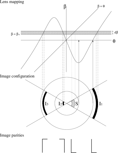
Figure 2: Illustration of the lens mapping $\beta=\beta(\theta)$ (upper panel), image configuration (middle panel), and image parities (lower panel) for a typical axis-symmetric lens system. Three images ($I_{1},I_{2},I_{3}$) are produced for a source ($S$) at the location $\beta=\beta_{s}$ with a radial width $\delta\beta$. The images are formed at the intersections of $\beta=\beta(\theta)$ and the horizontal line $\beta=\beta_{s}$. Critical curves are also shown by two solid concentric circles in the middle panel. The inner circle represents the radial critical curve where $d\beta(\theta)/d\theta=0$, while the outer circle represents the tangential critical curve where $\beta(\theta)=0$. The image parities are illustrated in the lower panel. The images $I_{1}$ and $I_{2}$ have the same total parity as the source $S$, while $I_{3}$ has the opposite total parity to $S$. The concepts of critical curves and image parities are given in Sect. 2.6.3.

In general, the lens equation is nonlinear with respect to the image position $\theta$, so that it may have multiple solutions $\theta$ for a given source position $\beta$. This corresponds to multiple imaging of a background source (see Hattori et al., 1999; Kneib and Natarajan, 2011). An illustration of the typical circularly symmetric lens system is shown in Fig. 2. We refer to Keeton (2001) for a review of various families of mass models for gravitational lensing.

2.3 Cosmological lens equation

Here we turn to the cosmological lens equation that describes the light propagation in a locally inhomogeneous, expanding universe. There are various approaches to derive a cosmological version of the lens equation (e.g., Schneider, 1985; Sasaki, 1993; Seitz et al., 1994; Futamase, 1995; Dodelson, 2003; Sereno, 2009). We follow the approach by Futamase (1995) based on perturbed null geodesic equations as introduced in Sect. 2.1.

Consider a perturbed Friedman–Lemaítre–Robertson–Walker (FLRW) metric in the Newtonian gauge of the form (e.g., Kodama and Sasaki, 1984):

$$ds^{2}=-(1+2\Psi/c^{2})c^{2}dt^{2}+(1-2\Psi/c^{2})a^{2}(t)\left[d\chi^{2}+r^{2}(d\vartheta^{2}+\sin^{2}\vartheta d\varphi^{2})\right],$$ (9)

where $a(t)$ is the scale factor of the universe (normalized to unity at present), $\chi$ is the comoving distance, $\vartheta$ and $\varphi$ are the spherical polar and azimuthal angles, respectively, $\Psi$ is a scalar metric perturbation, $K$ is the spatial curvature of the universe, and $r=f_{K}(\chi)$ is the comoving angular diameter distance:

$$f_{K}(\chi)=\begin{cases}(-K)^{-1/2}\sinh(\chi/\sqrt{-K})&(K<0),\\ \chi&(K=0),\\ K^{-1/2}\sin(\chi/\sqrt{K})&(K>0).\end{cases}$$ (10)

The spatial curvature $K$ is expressed with the total density parameter at the present epoch, $\mathrm{\Omega}_{0}\equiv\sum_{X}\mathrm{\Omega}_{X}=\mathrm{\Omega}_{\mathrm{m}}+\mathrm{\Omega}_{\mathrm{r}}+\mathrm{\Omega}_{\mathrm{\Lambda}}$, as $K=(\mathrm{\Omega}_{0}-1)H_{0}^{2}/c^{2}$. The evolution of $a(t)$ is determined by the Friedmann equation, $H(a)\equiv(da/dt)/a=H_{0}[\mathrm{\Omega}_{\mathrm{r}}a^{-4}+\mathrm{\Omega}_{\mathrm{m}}a^{-3}+\mathrm{\Omega}_{\mathrm{\Lambda}}+(1-\mathrm{\Omega}_{0})a^{-2}]^{1/2}$. In the line element (9), we have neglected all terms of higher than $O(\Psi/c^{2})$, the contributions from vector and tensor perturbations, and the effects due to anisotropic stress. As we will discuss in Sect. 2.5.1, $\Psi$ is interpreted as the Newtonian gravitational potential generated by local inhomogeneities of the matter distribution in the universe.

Since the structure of a light cone is invariant under the conformal transformation, we work with the conformally related spacetime metric given by $d\tilde{s}^{2}=a^{-2}ds^{2}\equiv\tilde{g}_{\mu\nu}dx^{\mu}dx^{\nu}$ with $(x^{\mu})=(\eta,\chi,\vartheta,\varphi)$, where $\eta=c\int^{t}\!dt^{\prime}/a(t^{\prime})$ is the conformal time. The metric $\tilde{g}_{\mu\nu}$ can be rewritten in the form of $\tilde{g}_{\mu\nu}=\tilde{g}^{(\mathrm{b})}_{\mu\nu}+h_{\mu\nu}$, as a sum of the background metric and a small perturbation ($|h|\ll 1$).

We follow the prescription given in Sect. 2.1 to solve the null geodesic equations in the perturbed spacetime (Eq. (9)). To this end, we consider past-directed null geodesics from the observer. Choosing the spherical coordinate system centered on the observer, we have $k^{(\mathrm{b})\mu}=(-1,1,0,0)$ in the background metric with $\Psi=0$. The unperturbed path is parameterized by the affine parameter $\lambda$ along the photon path as $x^{(\mathrm{b})\mu}(\lambda)=(-\lambda,\lambda-\lambda_{o},\vartheta_{I},\varphi_{I})$, where $\lambda_{o}$ is the affine parameter at the observer and $(\vartheta_{I},\varphi_{I})$ denote the angular direction of the image position on the sky. The comoving angular distance $r$ in the background spacetime can be parameterized by $\lambda$ as $r(\lambda)\equiv f_{K}[\chi(\lambda-\lambda_{o})]$ (see Eq. (10)).

The perturbed null geodesic equations for the angular components ($\vartheta,\varphi$) can be formally solved as:

$$\delta k^{i}(\lambda)=-\frac{2}{r^{2}(\lambda)}\int_{\lambda_{o}}^{\lambda_{s}}\!d\lambda^{\prime}\partial^{i}\Psi(\lambda^{\prime})/c^{2}\ \ \ (i=\vartheta,\varphi),$$ (11)

where $\partial^{i}\Psi=(\Psi_{,\vartheta},\sin^{-2}\vartheta\Psi_{,\varphi})$ and we have chosen $\delta k^{\vartheta}(\lambda_{o})=\delta k^{\varphi}(\lambda_{o})=0$. Inserting this result in Eq. (4) and integrating by part yield (Futamase, 1995; Dodelson, 2003):

$$\vartheta_{S} =\vartheta_{I}-\frac{2}{c^{2}}\int_{\lambda_{o}}^{\lambda_{s}}\!\frac{r(\lambda_{s}-\lambda)}{r(\lambda_{s})r(\lambda)}\partial^{\theta}\Psi(\lambda)\,d\lambda,$$ (12)

$$\varphi_{S} =\varphi_{I}-\frac{2}{c^{2}}\int_{\lambda_{o}}^{\lambda_{s}}\!\frac{r(\lambda_{s}-\lambda)}{r(\lambda_{s})r(\lambda)}\partial^{\varphi}\Psi(\lambda)\,d\lambda,$$

where $\lambda_{s}$ is the affine parameter at the background source, $(\vartheta_{S},\varphi_{S})\equiv(\vartheta(\lambda_{s}),\varphi(\lambda_{s}))$ denote the angular direction of the unlensed source position on the sky, and we set $\delta\vartheta(\lambda_{o})=\delta\varphi(\lambda_{o})=0$. Here, the integral is performed along the perturbed trajectory $x^{\mu}(\lambda)=x^{(\mathrm{b})\mu}(\lambda)+\delta x^{\mu}(\lambda)$. Equation (12) relates the observed direction of the image position $(\vartheta_{I},\varphi_{I})$ to the (unlensed) direction of the source position $(\vartheta_{S},\varphi_{S})$ for a given background cosmology and metric perturbation $\Psi(\mbox{\boldmath$\chi$},\eta)$. This is a general expression of the cosmological lens equation obtained by Futamase (1995).

2.4 Flat-sky approximation

Now we consider a small patch of the sky around a given line of sight ($\vartheta=0$), across which the curvature of the sky is negligible ($\vartheta\ll 1$). Then, we can locally define a flat plane perpendicular to the line of sight. By noting that $\delta\mbox{\boldmath$\theta$}\equiv(\delta\vartheta,\vartheta\delta\varphi)$ is an angular displacement vector within this sky plane, we can express Eq. (12) as:

$$\mbox{\boldmath$\beta$}(\chi_{s})=\mbox{\boldmath$\theta$}+\mbox{\boldmath$\alpha$}(\chi_{s}),$$ (13)

where $\mbox{\boldmath$\beta$}(\chi_{s})$ is the (unlensed) angular position of the source, $\theta$ is the apparent angular position of the source image, and $\mbox{\boldmath$\alpha$}(\chi_{s})$ is the deflection field given by (Futamase, 1995):

$$\mbox{\boldmath$\alpha$}(\chi_{s})=-\frac{2}{c^{2}}\int_{0}^{\chi_{s}}\!\frac{r(\chi_{s}-\chi)}{r(\chi_{s})}\mbox{\boldmath$\nabla$}_{\perp}\Psi[x^{\mu}(\chi)]\,d\chi,$$ (14)

where $\mbox{\boldmath$\nabla$}_{\perp}\equiv r^{-1}(\lambda)(\partial_{\vartheta},\vartheta^{-1}\partial_{\varphi})$ is the transverse comoving gradient and the integral is performed along the perturbed trajectory $x^{\mu}(\lambda)=x^{(\mathrm{b})\mu}(\lambda)+\delta x^{\mu}(\lambda)$ with $\lambda=\chi+O(\Psi/c^{2})$. Equation (13) can be applied to a range of lensing phenomena, including multiple deflections of light from a background source (Sect. 2.5), strong and weak gravitational lensing by individual galaxies and clusters (Sect. 2.6), and cosmological weak lensing by the intervening large-scale structure (a.k.a., the cosmic shear). Note that the cosmological lens equation is obtained using the standard angular diameter distance in a background FLRW spacetime without employing the thin-lens approximation (see Sect. 2.6).

2.5 Multiple lens equation

We consider a discretized version of the cosmological lens equation (Eq. (13)) by dividing the radial integral between the source ($\chi=\chi_{s}$) and the observer ($\chi=0$) into $N$ comoving boxes ($N-1$ lens planes) separated by a constant comoving distance of $\Delta\chi$. The angular position $\mbox{\boldmath$\theta$}^{(n)}$ of a light ray in the $n$th plane ($1\leqslant n\leqslant N$) is then given by (e.g., Schneider et al., 1992; Schneider, 2019):

$$\mbox{\boldmath$\beta$}^{(n)}=\mbox{\boldmath$\theta$}^{(0)}+\sum_{m=1}^{n-1}\frac{r(\chi_{n}-\chi_{m})}{r(\chi_{n})}\hat{\mbox{\boldmath$\alpha$}}^{(m)},$$ (15)

where $\mbox{\boldmath$\theta$}^{(0)}=\mbox{\boldmath$\beta$}^{(1)}$ is the apparent angular position of the source image and $\hat{\mbox{\boldmath$\alpha$}}^{(m)}$ is the bending angle at the $m$th lens plane ($m=1,2,\dots,n-1$):

$$\hat{\mbox{\boldmath$\alpha$}}^{(m)}=-\frac{2}{c^{2}}\mbox{\boldmath$\nabla$}_{\perp}\Psi[\chi_{m},r(\chi_{m})\mbox{\boldmath$\beta$}^{(m)}]\,\Delta\chi.$$ (16)

The $2\times 2$ Jacobian matrix of Eq. (15) ($1\leqslant n\leqslant N$) is expressed as (e.g., Jain et al., 2000):

$${\cal A}^{(n)}:=\frac{\partial\mbox{\boldmath$\beta$}^{(n)}}{\partial\mbox{\boldmath$\theta$}^{(0)}}={\cal I}+\sum_{m=1}^{n-1}\frac{D_{mn}}{D_{n}}{\cal H}^{(m)}{\cal A}^{(m)},$$ (17)

where ${\cal I}$ denotes the identity matrix, ${\cal H}^{(m)}\equiv\partial\hat{\mbox{\boldmath$\alpha$}}^{(m)}/\partial\mbox{\boldmath$\beta$}^{(m)}$ is a symmetric dimensionless Hessian matrix with ${\cal H}_{ij}^{(m)}=-(2/c^{2})r(\chi_{m})\nabla_{\perp,i}\nabla_{\perp,j}\Psi[\chi_{m},r(\chi_{m})\mbox{\boldmath$\beta$}^{(m)}]\,\Delta\chi$ ($i,j=1,2$), $D_{n}$ is the angular diameter distance between the observer and the $n$th lens plane, and $D_{mn}$ is the angular diameter distance between the $m$th and $n$th lens planes ($m<n$). In general, the Jacobian matrix ${\cal A}^{(n)}$ can be decomposed into the following form:

$${\cal A}^{(n)}=(1-\kappa){\cal I}-\gamma_{1}\sigma_{3}-\gamma_{2}\sigma_{1}-i\omega\sigma_{2},$$ (18)

where $\kappa$ is the lensing convergence, $(\gamma_{1},\gamma_{2})$ are the two components of the gravitational shear (see Sect. 2.6.2 for the definitions and further details of the convergence and shear), $\omega$ is the net rotation (e.g., Cooray and Hu, 2002), and $\sigma_{a}$ $(a=1,2,3)$ are the Pauli matrices that satisfy $\sigma_{a}\sigma_{b}=i\epsilon_{abc}\sigma_{c}$, with $\epsilon_{abc}$ the Levi–Civita symbol in three dimensions. The Born approximation ${\cal A}^{(m)}={\cal I}$ on the right-hand side of Eq. (17) leads to a symmetric Jacobian matrix with $\omega=0$.

The multiple lens equation has been widely used to study gravitational lensing phenomena by ray-tracing through $N$-body simulations (e.g., Schneider and Weiss, 1988; Hamana et al., 2000; Jain et al., 2000).

2.5.1 Cosmological poisson equation

We assume here a spatially flat geometry with $K=0$ motivated by cosmological observations based on cosmic microwave background (CMB) and complementary data sets (e.g., Hinshaw et al., 2013; Planck Collaboration et al., 2016b). The cosmological Poisson equation relates the scalar metric perturbation $\Psi$ (see Eq. (9)) to the matter density perturbation $\delta\rho$ on subhorizon scales as:

$$\mbox{\boldmath$\nabla$}^{2}\Psi(\mbox{\boldmath$\chi$},\eta)=4\pi Ga^{2}\delta\rho=\frac{3H_{0}^{2}\mathrm{\Omega}_{\mathrm{m}}}{2}\frac{\delta}{a},$$ (19)

where $\delta=\delta\rho/\overline{\rho}$ is the density contrast with respect to the background matter density $\overline{\rho}$ of the universe, $\overline{\rho}=a^{-3}(3H_{0}^{2}\mathrm{\Omega}_{\mathrm{m}})/(8\pi G)$, and $\nabla$ is the three-dimensional gradient operator in comoving coordinates. A key implication of Eq. (19) is that the amplitude of $\Psi$ is related to the amplitude of $\delta$ as $|\Psi/c^{2}|\sim(3\mathrm{\Omega}_{\mathrm{m}}/2)(l/L_{H})^{2}(\delta/a)$ where $l$ and $L_{H}=c/H_{0}$ denote the characteristic comoving scale of density perturbations and the Hubble radius, respectively. Therefore, assuming the standard matter power spectrum of density fluctuations (e.g., Smith et al., 2003), we can safely conclude that the degree of metric perturbation is always much smaller than unity, i.e., $|\Psi/c^{2}|\ll 1$, even for highly nonlinear perturbations with $|\delta|\gg 1$ on small scales of $l\ll L_{H}$ ($\sim 3h^{-1}\mathrm{Gpc}$).

2.6 Thin-lens equation

2.6.1 Thin-lens approximation

Let us turn to the case of gravitational lensing caused by a single cluster-scale halo. Galaxy clusters can produce deep gravitational potential wells, acting as powerful gravitational lenses. In cluster gravitational lensing it is often assumed that the total deflection angle, $\mbox{\boldmath$\alpha$}(\mbox{\boldmath$\theta$})$, is dominated by the cluster of interest and its surrounding large-scale environment, which becomes important beyond the cluster virial radius, $r_{\mathrm{vir}}$ (Cooray and Sheth, 2002; Oguri and Hamana, 2011; Diemer and Kravtsov, 2014).

Assuming that the light propagation is approximated by a single-lens event due to the cluster and that a light deflection occurs within a sufficiently small region ($\chi_{l}-\Delta\chi/2,\chi_{l}+\Delta\chi/2$) compared to the relevant angular diameter distances, we can write the deflection field by a single cluster as:

$$\mbox{\boldmath$\alpha$}(\mbox{\boldmath$\theta$})\simeq-\frac{2}{c^{2}}\frac{D_{ls}}{D_{s}}\int_{\chi_{l}-\Delta\chi/2}^{\chi_{l}+\Delta\chi/2}\!\mbox{\boldmath$\nabla$}_{\perp}\Psi[\chi,r(\chi_{l})\mbox{\boldmath$\theta$}]\,d\chi,$$ (20)

where $D_{s}=a(\chi_{s})r(\chi_{s})$ and $D_{ls}=a(\chi_{s})r(\chi_{s}-\chi_{l})$ are the angular diameter distances from the observer to the source and from the deflector to the source, respectively, and $r(\chi_{l})\mbox{\boldmath$\theta$}$ is the comoving transverse vector on the lens plane. In a cosmological situation, the angular diameter distances $D_{mn}$ between the planes $m$ and $n$ ($z_{m}<z_{n}$) are of the order of the Hubble radius, $L_{H}\equiv c/H_{0}\sim 3h^{-1}\mathrm{Gpc}$, while physical extents of clusters are about $2r_{\mathrm{200m}}\sim(2-4)h^{-1}\mathrm{Mpc}$ in comoving units. Therefore, one can safely adopt the thin-lens approximation in cluster gravitational lensing.

We then introduce the effective lensing potential $\psi(\mbox{\boldmath$\theta$})$ defined as:

$$\psi(\mbox{\boldmath$\theta$})\simeq\frac{2}{c^{2}}\frac{D_{ls}}{D_{l}D_{s}}\int_{\chi_{l}-\Delta\chi/2}^{\chi_{l}+\Delta\chi/2}\Psi[\chi,r(\chi_{l})\mbox{\boldmath$\theta$}]\,ad\chi,$$ (21)

where $D_{l}$ is the angular diameter distance between the observer and the lens, $D_{l}=a(\chi_{l})r(\chi_{l})$. In terms of $\psi(\mbox{\boldmath$\theta$})$, the deflection field $\mbox{\boldmath$\alpha$}(\theta)$ is expressed as:

$$\mbox{\boldmath$\alpha$}(\mbox{\boldmath$\theta$})=-\mbox{\boldmath$\nabla$}_{\theta}\psi(\mbox{\boldmath$\theta$}),$$ (22)

where $\mbox{\boldmath$\nabla$}_{\theta}=r\mbox{\boldmath$\nabla$}_{\perp}=(\partial_{\theta},\theta^{-1}\partial_{\phi})$.

With the Fermat or time-delay potential defined by:

$$\tau(\mbox{\boldmath$\theta$};\mbox{\boldmath$\beta$})\equiv\frac{1}{2}(\mbox{\boldmath$\theta$}-\mbox{\boldmath$\beta$})^{2}-\psi(\mbox{\boldmath$\theta$}),$$ (23)

the lens equation can be equivalently written as $\mbox{\boldmath$\nabla$}_{\theta}\tau(\mbox{\boldmath$\theta$};\mbox{\boldmath$\beta$})=0$ (Blandford and Narayan, 1986). Here the first term on the right hand side of Eq. (23) is responsible for the geometric delay and the second term for the gravitational time delay. The Fermat potential $\tau(\mbox{\boldmath$\theta$};\mbox{\boldmath$\beta$})$ is related to the time delay $\Delta t$ with respect to the unperturbed path in the observer frame by $\Delta t(\mbox{\boldmath$\theta$};\mbox{\boldmath$\beta$})=D_{l}D_{s}/(cD_{ls})(1+z_{l})\tau(\mbox{\boldmath$\theta$};\mbox{\boldmath$\beta$})\equiv D_{\Delta t}\tau(\mbox{\boldmath$\theta$};\mbox{\boldmath$\beta$})/c$. with $D_{\Delta t}=(1+z_{l})D_{l}D_{s}/D_{ls}\propto H_{0}^{-1}$ the time-delay distance (Refsdal, 1964). According to Fermat’s principle, the images for a given source position $\beta$ are formed at the stationary points of $\tau(\mbox{\boldmath$\theta$};\mbox{\boldmath$\beta$})$ with respect to variations of $\theta$ (Blandford and Narayan, 1986).

Note that cluster gravitational lensing is also affected by uncorrelated large-scale structure projected along the line of sight (e.g., Schneider et al., 1998; Hoekstra, 2003; Umetsu et al., 2011a; Host, 2012). The intervening large-scale structure in the universe perturbs the propagation of light from distant background galaxies, producing small but continuous transverse excursions along the light path. For a given depth of observations, the impact of such cosmic noise is most important in the cluster outskirts where the cluster lensing signal is small (Hoekstra, 2003; Becker and Kravtsov, 2011; Gruen et al., 2015).

2.6.2 Convergence and shear

Let us work with local Cartesian coordinates $\mbox{\boldmath$\theta$}=(\theta_{1},\theta_{2})$ centered on a certain reference point in the image plane. The local properties of the lens mapping are described by the Jacobian matrix defined as:

$${\cal A}(\mbox{\boldmath$\theta$}):=\frac{\partial\mbox{\boldmath$\beta$}}{\partial\mbox{\boldmath$\theta$}}=\left(\begin{array}[]{cc}1-\psi_{,11}&-\psi_{,12}\\ -\psi_{,12}&1-\psi_{,22}\end{array}\right),$$ (24)

where we have introduced the notation, $\psi_{,ij}=\partial^{2}\psi/\partial\theta_{i}\partial\theta_{j}$ ($i,j=1,2$). Alternatively, we can write the Jacobian matrix as ${\cal A}_{ij}=\delta_{ij}-\psi_{,ij}$ ($i,j=1,2$) with $\delta_{ij}$ the Kronecker delta in two dimensions. This symmetric $2\times 2$ Jacobian matrix ${\cal A}$ can be decomposed as:

$${\cal A}=(1-\kappa){\cal I}-\gamma_{1}\sigma_{3}-\gamma_{2}\sigma_{1},$$ (25)

where $\sigma_{a}$ $(a=1,2,3)$ are the Pauli matrices (Sect. 2.5); $\kappa(\mbox{\boldmath$\theta$})$ is the lensing convergence responsible for the change in the trace part of the Jacobian matrix ($\mathrm{tr}({\cal A})=2(1-\kappa)$):

$$\kappa:=\frac{1}{2}\left(\psi_{,11}+\psi_{,22}\right)=\frac{1}{2}\triangle\psi$$ (26)

with $\triangle=\mbox{\boldmath$\nabla$}_{\theta}^{2}$, and ($\gamma_{1},\gamma_{2}$) are the two components of the complex shear $\gamma(\mbox{\boldmath$\theta$}):=\gamma_{1}(\mbox{\boldmath$\theta$})+i\gamma_{2}(\mbox{\boldmath$\theta$})$:

$$\gamma_{1} :=\frac{1}{2}\left(\psi_{,11}-\psi_{,22}\right),$$ (27)

$$\gamma_{2} :=\frac{1}{2}\left(\psi_{,12}+\psi_{,21}\right)=\psi_{,12}.$$

Note that Eq. (26) can be regarded as a two-dimensional Poisson equation, $\triangle\psi(\mbox{\boldmath$\theta$})=2\kappa(\mbox{\boldmath$\theta$})$. Then, the Green function in the (hypothetical) infinite domain is $\triangle^{-1}(\mbox{\boldmath$\theta$},\mbox{\boldmath$\theta$}^{\prime})=\ln|\mbox{\boldmath$\theta$}-\mbox{\boldmath$\theta$}^{\prime}|/(2\pi)$, so that the convergence is related to the lensing potential as:

$$\psi(\mbox{\boldmath$\theta$})=\frac{1}{\pi}\int\!\ln(\mbox{\boldmath$\theta$}-\mbox{\boldmath$\theta$}^{\prime})\kappa(\mbox{\boldmath$\theta$}^{\prime})\,d^{2}\theta^{\prime}.$$ (28)

The Jacobian matrix is expressed in terms of $\kappa$ and $\gamma$ as:

$${\cal A}(\mbox{\boldmath$\theta$})=\left(\begin{array}[]{cc}1-\kappa-\gamma_{1}&-\gamma_{2}\\ -\gamma_{2}&1-\kappa+\gamma_{1}\end{array}\right).$$ (29)

The determinant of the Jacobian matrix (Eq. (29)) is given as $\mathrm{det}{\cal A}=(1-\kappa)^{2}-|\gamma|^{2}$. In the weak-lensing limit where $|\kappa|,|\gamma|\ll 1$, $\mathrm{det}{\cal A}\simeq 1-2\kappa$ to the first order.

The deformation of the image of an infinitesimal circular source ($d\mbox{\boldmath$\beta$}\to 0$) behind the lens can be described by the inverse Jacobian matrix ${\cal A}^{-1}$ of the lens equation. In the weak-lensing limit ($|\kappa|,|\gamma|\ll 1$), we have:

$$\left({\cal A}^{-1}\right)_{ij}\simeq(1+\kappa)\delta_{ij}+{\Gamma}_{ij}\ \ \ (i,j=1,2),$$ (30)

where $\Gamma_{ij}$ is the symmetric trace-free shear matrix defined by (Bartelmann and Schneider, 2001; Crittenden et al., 2002):

$$\Gamma_{ij}=\left(\partial_{i}\partial_{j}-\delta_{ij}\frac{1}{2}\triangle\right)\psi(\mbox{\boldmath$\theta$}),$$ (31)

with $\partial_{i}:=\partial/\partial\theta_{i}$ ($i=1,2$). The shear matrix can be expressed in terms of the Pauli matrices as $\Gamma=\sigma_{3}\gamma_{1}+\sigma_{1}\gamma_{2}$. The first term in Eq. (30) describes the isotropic light focusing or area distortion in the weak-lensing limit, while the second term induces an asymmetry in lens mapping. The shear $\gamma$ is responsible for image distortion and can be directly observed from image ellipticities of background galaxies in the regime where $|\kappa|,|\gamma|\ll 1$ (see Sect. 3). Note that both $\kappa$ and $\gamma$ contribute to the area and shape distortions in the non-weak-lensing regime.

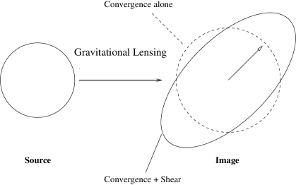
Figure 3: Illustration of the effects of the convergence $\kappa$ and the shear $\gamma$ on the angular shape and size of a hypothetical circular source. The convergence acting alone causes an isotropic focusing (magnification) of the image (dashed circle), while the shear deforms it to an ellipse.

In Fig. 3, we illustrate the effects of the lensing convergence $\kappa$ and the gravitational shear $\gamma$ on the angular shape and size of an infinitesimal circular source. The convergence acting alone causes an isotropic magnification of the image, while the shear deforms it to an ellipse. Note that the magnitude of ellipticity induced by gravitational shear in the weak-lensing regime ($|\gamma|\lower 2.15277pt\hbox{$\;\buildrel<\over{\sim}\;$}0.1$) is much smaller than illustrated here.

2.6.3 Magnification

Gravitational lensing describes the deflection of light by gravity. Lensing conserves the surface brightness of a background source, a consequence of Liouville’s theorem. On the other hand, lensing causes focusing of light rays, resulting in an amplification of the image flux through the local solid-angle distortion. Lensing magnification $\mu$ is thus given by taking the ratio between the lensed to the unlensed image solid angle as $\mu=\delta\Omega^{I}/\delta\Omega^{S}=1/\mathrm{det}{\cal A}$, with:

$$\mu(\mbox{\boldmath$\theta$})=\frac{1}{[1-\kappa(\mbox{\boldmath$\theta$})]^{2}-|\gamma(\mbox{\boldmath$\theta$})|^{2}}.$$ (32)

In the weak-lensing limit ($|\kappa|,|\gamma|\ll 1$), the magnification factor to the first order is:

$$\mu(\mbox{\boldmath$\theta$})\simeq 1+2\kappa(\mbox{\boldmath$\theta$}).$$ (33)

The magnitude change at $\kappa(\mbox{\boldmath$\theta$})=0.1$ is thus $\Delta m=-(5/2)\log_{10}(\mu)\sim-0.2$.

2.6.4 Strong- and weak-lensing regimes

The ${\cal A}(\mbox{\boldmath$\theta$})$ matrix has two local eigenvalues $\Lambda_{\pm}(\mbox{\boldmath$\theta$})$ at each image position $\theta$:

$$\Lambda_{\pm}=1-\kappa\pm|\gamma|,$$ (34)

with $\Lambda_{+}\geqslant\Lambda_{-}$.

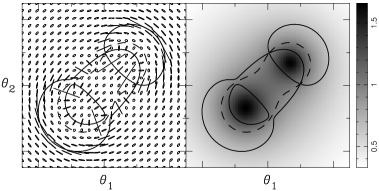
Figure 4: Shape distortion field produced by a simulated lens with a bimodal mass distribution. At each grid point in the image plane (left panel), we have drawn the apparent shape for an intrinsically circular source using the local deformation factors $\Lambda_{\pm}$ (Eq. (34)). All ellipses have an equal area regardless of the magnification factor. The right panel shows the $\kappa$ map of the bimodal lens. In both panels, the solid lines indicate the critical curves. The image distortion disappears locally along the curve $\kappa=1$ indicated by the dashed line, which lies in the negative-parity region.

Images with $\mathrm{det}{\cal A}(\mbox{\boldmath$\theta$})>0$ have the same parity as the source, while those with $\mathrm{det}{\cal A}(\mbox{\boldmath$\theta$})<0$ have the opposite parity to the source. A set of closed curves defined by $\mathrm{det}{\cal A}(\mbox{\boldmath$\theta$})=0$ in the image plane are referred to as critical curves, on which lensing magnification formally diverges, and those mapped into the source plane are referred to as caustics (see Hattori et al., 1999). The critical curves separate the image plane into even- and odd-parity regions with $\mathrm{det}{\cal A}>0$ and $\mathrm{det}{\cal A}<0$, respectively.

An infinitesimal circular source is transformed to an ellipse with a minor-to-major axis ratio ($\leqslant 1$) of $|\Lambda_{-}/\Lambda_{+}|$ for $\kappa<1$ and $|\Lambda_{+}/\Lambda_{-}|$ for $\kappa>1$, and it is magnified by the factor $|\mu|=1/|\Lambda_{+}\Lambda_{-}|$ (see Sect. 2.6.3). The gravitational distortion locally disappears along the curve defined by $\mathrm{tr}[{\cal A}(\mbox{\boldmath$\theta$})]=0$, i.e., $\kappa(\mbox{\boldmath$\theta$})=1$, which lies in the odd-parity region (Kaiser, 1995). This is illustrated in Fig. 4 for a simulated lens with a bimodal mass distribution. Images forming along the outer (tangential) critical curve $\Lambda_{-}(\mbox{\boldmath$\theta$})=0$ are distorted tangentially to this curve, while images forming close to the inner (radial) critical curve $\Lambda_{+}(\mbox{\boldmath$\theta$})=0$ are stretched in the direction perpendicular to the critical curve.

A lens system that has a region with $\kappa(\mbox{\boldmath$\theta$})>1$ can produce multiple images for certain source positions $\beta$, and such a system is referred to as being supercritical. Note that being supercritical is a sufficient but not a necessary condition for a general lens to produce multiple images, because the shear can also contribute to multiple imaging. Nevertheless, this provides us with a simple criterion to broadly distinguish the regimes of multiple and single imaging. Keeping this in mind, we refer to the region where $\kappa(\mbox{\boldmath$\theta$})\lower 2.15277pt\hbox{$\;\buildrel>\over{\sim}\;$}1$ as the strong-lensing regime and the region where $\kappa(\mbox{\boldmath$\theta$})\ll 1$ as the weak-lensing regime.

2.6.5 Critical surface mass density

The lensing convergence $\kappa$ is essentially a distance-weighted mass overdensity projected along the line of sight. We express $\kappa(\mbox{\boldmath$\theta$})$ due to cluster gravitational lensing as:

$$\kappa(\mbox{\boldmath$\theta$})=\int_{0}^{\chi_{s}}\!(\rho-\overline{\rho})\left(\frac{c^{2}}{4\pi G}\frac{D_{s}}{D_{l}D_{ls}}\right)^{-1}ad\chi\simeq\frac{\Sigma(\mbox{\boldmath$\theta$})}{\Sigma_{\mathrm{cr}}},$$ (35)

where $\chi_{s}$ is the comoving distance to the source plane; $\Sigma=\int_{0}^{\chi_{s}}\!(\rho-\overline{\rho})\,ad\chi$ is the surface mass density field of the lens projected on the sky; and $\Sigma_{\mathrm{cr}}$ is the critical surface mass density of gravitational lensing:

$$\Sigma_{\mathrm{cr}}(z_{l},z_{s}) =\frac{c^{2}}{4\pi G}\frac{D_{s}}{D_{l}D_{ls}}$$ (36)

for $z_{s}>z_{l}$ and $\Sigma_{\mathrm{cr}}^{-1}(z_{l},z_{s})=0$ (i.e., $D_{ls}/D_{s}=0$) for an unlensed source with $z_{s}\leqslant z_{l}$. In the second (approximate) equality of Eq. (35), we have explicitly used the thin-lens approximation (Sect. 2.6.1). The critical surface mass density $\Sigma_{\mathrm{cr}}$ depends on the geometric configuration ($z_{l},z_{s}$) of the lens–source system and the background cosmological parameters, such as ($\mathrm{\Omega}_{\mathrm{m}},\mathrm{\Omega}_{\mathrm{\Lambda}},H_{0}$). For example, for $z_{l}=0.3$ and $z_{s}=1$ in our fiducial cosmology, we have $\Sigma_{\mathrm{cr}}\approx 4.0\times 10^{15}hM_{\odot}$ Mpc^-2. For a fixed lens redshift $z_{l}$, the geometric efficiency of gravitational lensing is determined by the distance ratio $D_{ls}/D_{s}$ as a function of $z_{s}$ and the background cosmology.

Figure 5: Distance ratio $D_{ls}/D_{s}$ as a function of the source redshift $z_{s}$ for various sets of the lens redshift $z_{l}$ and the cosmological parameters $(\mathrm{\Omega}_{\mathrm{m}},\mathrm{\Omega}_{\mathrm{\Lambda}})$. The ratio $D_{ls}/D_{s}$ is shown for three different lens redshifts, $z_{l}=0.2,0.5$, and $0.8$ (from left to right) and for three sets of the cosmological parameters, $(\mathrm{\Omega}_{\mathrm{m}},\mathrm{\Omega}_{\mathrm{\Lambda}})=(1,0),(0.3,0)$, and $(0.3,0.7)$.

To translate the observed lensing signal into surface mass densities, one needs an estimate of $\Sigma_{\mathrm{cr}}(z_{l},z_{s})$ for a given background cosmology. In the regime where $z_{l}\ll z_{s}$ (say, $z_{l}\lower 2.15277pt\hbox{$\;\buildrel<\over{\sim}\;$}0.2$ for background galaxy populations at $z_{s}\sim 1$), $\Sigma_{\mathrm{cr}}$ depends weakly on the source redshift $z_{s}$, so that a precise knowledge of the source-redshift distribution is less critical (e.g., Okabe and Umetsu, 2008; Okabe et al., 2010).

Conversely, this distance dependence of the lensing effects can be used to constrain the cosmological redshift–distance relation by examining the geometric scaling of the lensing signal as a function of the background redshift (Taylor et al., 2007, 2012; Medezinski et al., 2011; Dell’Antonio et al., 2019). Figure 5 compares $D_{ls}/D_{s}$ as a function of $z_{s}$ for various sets of the lens redshift and the cosmological model.

Note that, in the limit where the lensing matter is continuously distributed along the line of sight, the first equality of Eq. (35) can be formally rewritten as:

$$\kappa(\mbox{\boldmath$\theta$})=\frac{3H_{0}^{2}}{2c^{2}}\mathrm{\Omega}_{\mathrm{m}}\int_{0}^{\chi_{s}}\!d\chi\,g(\chi,\chi_{s})a^{-1}(\chi)\delta[\chi,r(\chi)\mbox{\boldmath$\theta$}],$$ (37)

with $g(\chi,\chi_{s})=r(\chi)r(\chi_{s}-\chi)/r(\chi_{s})$ and $\delta=\delta\rho/\overline{\rho}$. Equation (37) coincides with the expression for the cosmic convergence due to intervening cosmic structures (see Jain et al., 2000). It is interesting to compare the above line-of-sight integral (Eq. (37)) to the thermal Sunyaev–Zel’dovich effect (SZE) in terms of the Compton-$y$ parameter (e.g., Sunyaev and Zeldovich, 1972; Rephaeli, 1995; Birkinshaw, 1999):

$$y=\frac{\sigma_{\mathrm{T}}}{m_{\mathrm{e}}c^{2}}\int\!n_{\mathrm{e}}k_{\mathrm{B}}\left(T_{\mathrm{e}}-T_{\mathrm{CMB}}\right)\,cdt\simeq\frac{\sigma_{\mathrm{T}}}{m_{\mathrm{e}}c^{2}}\int\!P_{\mathrm{e}}\,cdt,$$ (38)

where $\sigma_{\mathrm{T}}$, $m_{\mathrm{e}}$, $k_{\mathrm{B}}$ are the Thomson scattering cross-section, the electron mass, and the Boltzmann constant, respectively; $T_{\mathrm{CMB}}=T_{0}(1+z)$ is the temperature of CMB photons with $T_{0}=2.725$ K; and $T_{e}$ and $n_{e}$ are the electron temperature and number density of the intracluster gas, with $P_{\mathrm{e}}=n_{\mathrm{e}}k_{\mathrm{B}}T_{\mathrm{e}}$ the electron pressure. In the second (approximate) equality, we have used $T_{e}\gg T_{0}(1+z)$. The Compton-$y$ parameter is proportional to the electron pressure integrated along the line of sight, thus probing the thermal energy content of thermalized hot plasmas residing in the gravitational potential wells of galaxy clusters. The combination of the thermal SZE and weak lensing thus provides unique astrophysical and cosmological probes (e.g., Doré et al., 2001; Umetsu et al., 2009; Osato et al., 2020).

2.6.6 Einstein radius

Detailed strong-lens modeling using many sets of multiple images with measured spectroscopic redshifts allows us to determine the location of the critical curves (e.g., Zitrin et al., 2015; Meneghetti et al., 2017), which, in turn, provides accurate estimates of the projected total mass enclosed by them. In this context, the term Einstein radius is often used to refer to the size of the outer (tangential) critical curve (i.e., $\Lambda_{-}(\mbox{\boldmath$\theta$})=0$; Sect. 2.6.4). We note, however, that there are several possible definitions of the Einstein radius used in the literature (see Meneghetti et al., 2013). Here we adopt the effective Einstein radius definition (Redlich et al., 2012; Meneghetti et al., 2013, 2017; Zitrin et al., 2015), $\vartheta_{\mathrm{Ein}}=\sqrt{A_{\mathrm{c}}/\pi}$, where $A_{\mathrm{c}}$ is the (angular) area enclosed by the outer critical curve. For an axisymmetric lens, the average surface mass density within the critical area is equal to $\Sigma_{\mathrm{cr}}$ (see Hattori et al., 1999; Meneghetti et al., 2013), thus enabling us to directly estimate the enclosed projected mass by $M_{\mathrm{2D}}(<\vartheta_{\mathrm{Ein}})=\pi(D_{l}\vartheta_{\mathrm{Ein}})^{2}\Sigma_{\mathrm{cr}}$. Even for general non-axisymmetric lenses, the projected enclosed mass profile $M_{\mathrm{2D}}(<\vartheta)=\Sigma_{\mathrm{cr}}D_{l}^{2}\int_{\vartheta^{\prime}\leq\vartheta}\!\kappa(\mbox{\boldmath$\theta$}^{\prime})\,d^{2}\theta^{\prime}$ at the location $\vartheta\sim\vartheta_{\mathrm{Ein}}$ is less sensitive to modeling assumptions and approaches (e.g., Umetsu et al., 2012, 2016; Meneghetti et al., 2017), thus serving as a fundamental observable quantity in the strong-lensing regime (Coe et al., 2010).

3 Basics of cluster weak lensing

In this section, we review the basics of cluster–galaxy weak lensing based on the thin-lens formalism (Sect. 2.6). Unless otherwise noted, we will focus on subcritical lensing (i.e., outside the critical curves). We consider both linear ($\kappa\ll 1$) and mildly nonlinear regimes of weak gravitational lensing.

3.1 Weak-lensing mass reconstruction

3.1.1 Spin operator and lensing fields

For mathematical convenience, we introduce a concept of “spin” for weak-lensing quantities as follows (Bacon et al., 2006; Okura et al., 2007, 2008; Schneider and Er, 2008; Bacon and Schäfer, 2009): a quantity is said to have spin $N$ if it has the same value after rotation by $2\pi/N$. The product of spin-$A$ and spin-$B$ quantities has spin ($A+B$), and the product of spin-$A$ and spin-$B^{*}$ quantities has spin ($A-B$), where $*$ denotes the complex conjugate.

We define a complex spin-1 operator $\partial:=\partial_{1}+i\partial_{2}$ that transforms as a vector, $\partial^{\prime}=\partial e^{i\varphi}$, with $\varphi$ being the angle of rotation relative to the original basis. Then, the lensing convergence is expressed in terms of $\psi(\mbox{\boldmath$\theta$})$ as:

$$\kappa(\mbox{\boldmath$\theta$})=\frac{1}{2}\partial^{*}\partial\psi(\mbox{\boldmath$\theta$}),$$ (39)

where $\partial\partial^{*}=\nabla_{\theta}^{2}$ is a scalar or a spin-0 operator. Similarly, the complex shear $\gamma=\gamma_{1}+i\gamma_{2}\equiv|\gamma|e^{2i\phi_{\gamma}}$ is expressed as:

$$\gamma(\mbox{\boldmath$\theta$})=\frac{1}{2}\partial\partial\psi(\mbox{\boldmath$\theta$})=\hat{\cal D}\psi(\mbox{\boldmath$\theta$}),$$ (40)

where

$$\hat{\cal D}:=\partial\partial/2=(\partial_{1}^{2}-\partial_{2}^{2})/2+i\partial_{1}\partial_{2}$$ (41)

is a spin-2 operator that transforms such that $\hat{\cal D^{\prime}}=\hat{\cal D}e^{2i\varphi}$ under a rotation of the basis axes by $\varphi$.

3.1.2 Linear mass reconstruction

Since $\gamma(\mbox{\boldmath$\theta$})$ and $\kappa(\mbox{\boldmath$\theta$})$ are both linear combinations of the second derivatives of $\psi(\mbox{\boldmath$\theta$})$, they are related to each other by (Kaiser, 1995; Crittenden et al., 2002; Umetsu, 2010):

$$\triangle\kappa(\mbox{\boldmath$\theta$})=\partial^{*}\partial^{*}\gamma(\mbox{\boldmath$\theta$})=2\hat{\cal D}^{*}\gamma(\mbox{\boldmath$\theta$}).$$ (42)

The shear-to-mass inversion can thus be formally expressed as:

$$\kappa(\mbox{\boldmath$\theta$})=\triangle^{-1}(\mbox{\boldmath$\theta$},\mbox{\boldmath$\theta$}^{\prime})\left[\partial^{*}\partial^{*}\gamma(\mbox{\boldmath$\theta$}^{\prime})\right]=2{\hat{\cal D}^{*}}\left(\triangle^{-1}(\mbox{\boldmath$\theta$},\mbox{\boldmath$\theta$}^{\prime})\left[\gamma(\mbox{\boldmath$\theta$}^{\prime})\right]\right).$$ (43)

Using $\triangle^{-1}(\mbox{\boldmath$\theta$},\mbox{\boldmath$\theta$}^{\prime})=\ln|\mbox{\boldmath$\theta$}-\mbox{\boldmath$\theta$}^{\prime}|/(2\pi)$ (Sect. 2.6.2), Eq. (43) in the flat-sky limit can be solved to yield the following nonlocal relation between $\kappa$ and $\gamma$ (Kaiser and Squires, 1993, hereafter KS93):

$$\kappa(\mbox{\boldmath$\theta$})-\kappa_{0}=\frac{1}{\pi}\int\!d^{2}\theta^{\prime}\,D^{*}(\mbox{\boldmath$\theta$}-\mbox{\boldmath$\theta$}^{\prime})\gamma(\mbox{\boldmath$\theta$}^{\prime}),$$ (44)

where $\kappa_{0}$ is an additive constant and $D(\mbox{\boldmath$\theta$})$ is a complex kernel defined as:

$$D(\mbox{\boldmath$\theta$})\equiv 2\pi\hat{\cal D}\left[\triangle^{-1}(\mbox{\boldmath$\theta$})\right]=\frac{\theta_{2}^{2}-\theta_{1}^{2}-2i\theta_{1}\theta_{2}}{|\theta|^{4}}=-\frac{1}{(\theta_{1}-i\theta_{2})^{2}}.$$ (45)

Similarly, the complex shear field can be expressed in terms of the convergence $\kappa$ as:

$$\gamma(\mbox{\boldmath$\theta$})=\frac{1}{\pi}\int\!d^{2}\theta^{\prime}\,D(\mbox{\boldmath$\theta$}-\mbox{\boldmath$\theta$}^{\prime})\kappa(\mbox{\boldmath$\theta$}^{\prime}).$$ (46)

This linear mass inversion formalism is often referred to as the KS93 algorithm.

It is computationally faster to work in Fourier domain (Jain et al., 2000) using the fast Fourier transform algorithm. By taking the Fourier transform of Eq. (42), we have a mass inversion relation in the conjugate Fourier space as:

$$\kappa(\mbox{\boldmath$\theta$}) =\int\!\frac{d^{2}k}{(2\pi)^{2}}\,\hat{\kappa}(\mbox{\boldmath$k$})e^{i\mbox{\boldmath$k$}\cdot\mbox{\boldmath$\theta$}},$$ (47)

$$\hat{\kappa}(\mbox{\boldmath$k$}) =\frac{k_{1}^{2}-k_{2}^{2}-2ik_{1}k_{2}}{k_{1}^{2}+k_{2}^{2}}\hat{\gamma}(\mbox{\boldmath$k$})\ \ \ (\mbox{\boldmath$k$}\neq 0),$$

where $k$ is the two-dimensional wave vector conjugate to $\theta$, and $\hat{\kappa}(\mbox{\boldmath$k$})$ and $\hat{\gamma}(\mbox{\boldmath$k$})$ are the Fourier transforms of $\kappa(\mbox{\boldmath$\theta$})$ and $\gamma(\mbox{\boldmath$\theta$})=\gamma_{1}(\mbox{\boldmath$\theta$})+i\gamma_{2}(\mbox{\boldmath$\theta$})$, respectively. In practical applications, one may assume $\hat{\kappa}(0)=0$ if the angular size of the observed shear field is sufficiently large, so that the mean convergence across the data field is approximated to zero. Otherwise, one must explicitly account for the boundary conditions imposed by the observed shear field to perform a mass reconstruction on a finite field (e.g., Kaiser, 1995; Seitz and Schneider, 1996; Bartelmann et al., 1996; Seitz and Schneider, 1997; Umetsu and Futamase, 2000).

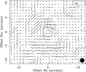
Figure 6: Shape distortion field in the rich cluster Cl0024+1654 ($z_{l}=0.395$) obtained from deep weak-lensing observations taken with Subaru/Suprime-Cam. The mean surface number density of background galaxies after the color–color selection (Sect. 4.1) is $n_{\mathrm{g}}=17.2$ arcmin^-2. A stick with a length of 10% shear is indicated in the top right corner. The filled circle indicates the FWHM ($1.4$ arcmin) of the Gaussian smoothing. The distortion field exhibits a coherent tangential pattern around the cluster center. Image reproduced with permission from Umetsu et al. (2010), copyright by AAS.

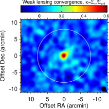
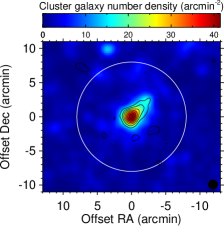
Figure 7: Comparison of mass and galaxy distributions in the rich cluster Cl0024+1654 ($z_{l}=0.395$). Left panel: projected mass distribution $\kappa(\mbox{\boldmath$\theta$})=\Sigma(\mbox{\boldmath$\theta$})/\Sigma_{\mathrm{cr}}$ reconstructed from deep weak-lensing data (Fig. 6) taken with Subaru/Suprime-Cam. Right panel: surface number density distribution $\Sigma_{n}(\mbox{\boldmath$\theta$})$ of color–color-selected cluster member galaxies. The solid circle in each panel indicates the cluster virial radius of $r_{\mathrm{vir}}\approx 1.8h^{-1}\mathrm{Mpc}$. Both maps are smoothed with a Gaussian of $1.4^{\prime}$ FWHM. Also overlaid on the $\Sigma_{n}$ map is the $\kappa(\mbox{\boldmath$\theta$})$ field shown in the left panel, given in units of $2\sigma$ reconstruction error from the lowest contour level of $3\sigma$. North is to the top, east to the left. Image reproduced with permission from Umetsu et al. (2010), copyright by AAS.

In Fig. 6, we show the shape distortion field in the rich cluster Cl0024+1654 ($z_{l}=0.395$) obtained by Umetsu et al. (2010) from deep weak-lensing observations taken with Suprime-Cam on the 8.2 m Subaru telescope. They accounted and corrected for the effect of the weight function used for calculating noisy galaxy shapes, as well as for the anisotropic and smearing effects of the point spread function (PSF), using an improved implementation of the modified Kaiser et al. (1995, hereafter KSB) method (see Sect. 3.4.2). In the left panel of Fig. 7, we show the $\kappa(\mbox{\boldmath$\theta$})$ field reconstructed from the Subaru weak-lensing data (see Fig. 6). A prominent mass peak is visible in the cluster center, around which the distortion pattern is clearly tangential (Fig. 6). In this study, a variant of the linear KS93 algorithm was used to reconstruct the $\kappa$ map from the weak shear lensing data. In the right panel of Fig. 7, we show the member galaxy distribution $\Sigma_{n}(\mbox{\boldmath$\theta$})$ in the cluster. Overall, mass and light are similarly distributed in the cluster.

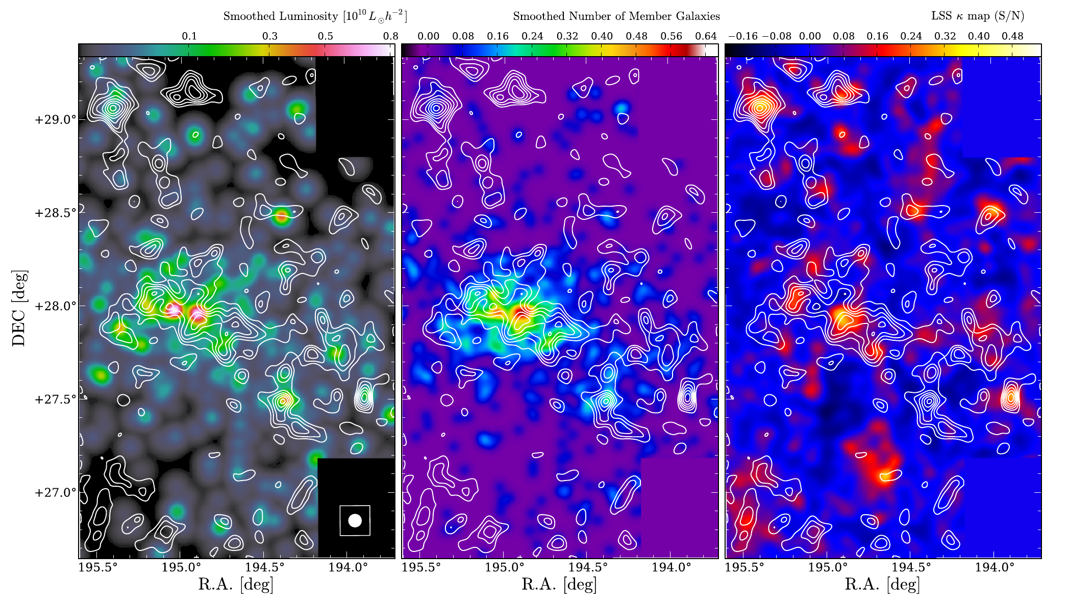
Figure 8: Projected mass distribution (contours) in the Coma cluster at $z=0.0236$ reconstructed from a $4$ deg² weak-lensing survey with Subaru Suprime-Cam observations. Left and middle panels: luminosity and number density distributions of spectroscopically identified cluster members, respectively. Right panel: projected large-scale structure model based on galaxy–galaxy lensing results. The mean surface number density of background galaxies after the color–magnitude selection is $n_{\mathrm{g}}=41.3$ arcmin^-2. Image reproduced with permission from Okabe et al. (2014), copyright by AAS.

Figure 8 shows the projected mass distribution in the very nearby Coma cluster ($z_{l}=0.0236$) reconstructed from a $4$ deg² weak-lensing survey of cluster subhalos based on Subaru Suprime-Cam observations (Okabe et al., 2014). In the figure, the weak-lensing mass map is compared to the luminosity and number density distributions of spectroscopically identified cluster members, as well as to the projected large-scale structure model based on galaxy–galaxy lensing with the light-tracing-mass assumption. The projected mass and galaxy distributions in the Coma cluster are correlated well with each other. Thanks to the large angular extension of the Coma cluster, Okabe et al. (2014) measured the weak-lensing masses of 32 cluster subhalos down to the order of $10^{-3}$ of the cluster virial mass.

3.1.3 Mass-sheet degeneracy

Adding a constant mass sheet to $\kappa(\mbox{\boldmath$\theta$})$ in the shear-to-mass formula (46) does not change the shear field $\gamma(\mbox{\boldmath$\theta$})$ that is observable in the weak-lensing limit. This leads to a degeneracy of solutions for the weak-lensing mass inversion problem, which is referred to as the mass-sheet degeneracy (Falco et al., 1985; Gorenstein et al., 1988; Schneider and Seitz, 1995).

As we shall see in Sect. 3.4, in general, the observable quantity for weak shear lensing is not the shear $\gamma$, but the reduced shear:

$$g(\mbox{\boldmath$\theta$})=\frac{\gamma(\mbox{\boldmath$\theta$})}{1-\kappa(\mbox{\boldmath$\theta$})}$$ (48)

in the subcritical regime where $\mathrm{det}{\cal A}>0$ (or $1/g^{*}$ in the negative-parity region with $\mathrm{det}{\cal A}<0$). We see that the $g(\mbox{\boldmath$\theta$})$ field is invariant under the following global transformation:

$$\kappa(\mbox{\boldmath$\theta$})\to\lambda\kappa(\mbox{\boldmath$\theta$})+1-\lambda,\ \ \ \gamma(\mbox{\boldmath$\theta$})\to\lambda\gamma(\mbox{\boldmath$\theta$})$$ (49)

with an arbitrary scalar constant $\lambda\neq 0$ (Schneider and Seitz, 1995). This transformation is equivalent to scaling the Jacobian matrix ${\cal A}(\mbox{\boldmath$\theta$})$ with $\lambda$, $\cal{A}(\mbox{\boldmath$\theta$})\to\lambda{\cal A}(\mbox{\boldmath$\theta$})$. It should be noted that this transformation leaves the location of the critical curves ($\mathrm{det}{\cal A}(\mbox{\boldmath$\theta$})=0$) invariant as well. Moreover, the location of the curve defined by $\kappa(\mbox{\boldmath$\theta$})=1$, on which the distortion locally disappears, is left invariant under the transformation (Eq. (49)). A general conclusion is that all mass reconstruction methods based on shape information alone can determine the $\kappa$ field only up to a one-parameter family ($\lambda$ or $\kappa_{0}$) of linear transformations (Eq. (49)).

In principle this degeneracy can be broken or alleviated, for example, by measuring the magnification factor $\mu$ in the subcritical regime (i.e., outside the critical curves; see Umetsu, 2013), because $\mu$ transforms under the invariance transformation (Eq. (49)) as:

$$\mu(\mbox{\boldmath$\theta$})\to\lambda^{-2}\mu(\mbox{\boldmath$\theta$}).$$ (50)

3.1.4 Nonlinear mass reconstruction

Following Seitz and Schneider (1995), we generalize the KS93 algorithm to include the nonlinear but subcritical regime (outside the critical curves). To this end, we express the KS93 inversion formula in terms of the observable reduced shear $g(\mbox{\boldmath$\theta$})$. Substituting $\gamma=g(1-\kappa)$ in Eq. (44), we have the following integral equation:

$$\kappa(\vec{\theta})-\kappa_{0}=\frac{1}{\pi}\int\!d^{2}\theta^{\prime}\,D^{*}(\mbox{\boldmath$\theta$}-\mbox{\boldmath$\theta$}^{\prime})\,g(\mbox{\boldmath$\theta$}^{\prime})\,[1-\kappa(\mbox{\boldmath$\theta$}^{\prime})].$$ (51)

For a given $g(\mbox{\boldmath$\theta$})$ field, this nonlinear equation can be solved iteratively, for example, by initially setting $\kappa(\mbox{\boldmath$\theta$})=0$ everywhere (Seitz and Schneider, 1995),

Equivalently, Eq. (51) can be formally expressed as a power series expansion (Umetsu et al., 1999):

$$\kappa(\mbox{\boldmath$\theta$})-\kappa_{0} =(1-\kappa_{0})\left(\hat{\cal G}-\hat{\cal G}\circ\!\hat{\cal G}+\hat{\cal G}\circ\!\hat{\cal G}\!\circ\!\hat{\cal G}-\cdots\right)$$ (52)

$$=(1-\kappa_{0})\sum_{n=1}^{\infty}(-1)^{n-1}\hat{\cal G}^{n},$$

where $\hat{\cal G}$ is the convolution operator defined by:

$$\hat{\cal G}(\mbox{\boldmath$\theta$},\mbox{\boldmath$\theta$}^{\prime}):=\frac{1}{\pi}\int\!d^{2}\theta^{\prime}\,D^{*}(\mbox{\boldmath$\theta$}-\mbox{\boldmath$\theta$}^{\prime})g(\mbox{\boldmath$\theta$}^{\prime})\,\times.$$ (53)

Here $\hat{\cal G}(\vec{\theta},\vec{\theta}^{\prime})$ acts on a function of $\mbox{\boldmath$\theta$}^{\prime}$. The KS93 algorithm corresponds to the first-order approximation to this power series expansion in the weak-lensing limit. Note that solutions for nonlinear mass reconstructions suffer from the generalized mass-sheet degeneracy, as explicitly shown in Eq.  (52).

Note that there is another class of mass inversion algorithms that uses maximum-likelihood and Bayesian approaches to obtain a mass map solution and its error covariance matrix from weak-lensing data (e.g., Bartelmann et al., 1996; Bradač et al., 2006; Merten et al., 2009).

3.2 $E/B$ decomposition

The shear matrix $\Gamma(\mbox{\boldmath$\theta$})=\gamma_{1}(\mbox{\boldmath$\theta$})\sigma_{3}+\gamma_{2}(\mbox{\boldmath$\theta$})\sigma_{1}$ that describes a spin-2 anisotropy can be expressed as a sum of two components corresponding to the number of degrees of freedom. By introducing two scalar fields $\psi_{E}(\mbox{\boldmath$\theta$})$ and $\psi_{B}(\mbox{\boldmath$\theta$})$, we decompose the shear matrix $\Gamma_{ij}$ ($i,j=1,2$) into two independent modes as (Crittenden et al., 2002):

$$\Gamma(\mbox{\boldmath$\theta$})=\left(\begin{array}[]{cc}\gamma_{1}&\gamma_{2}\\ \gamma_{2}&-\gamma_{1}\end{array}\right)=\Gamma^{(E)}(\mbox{\boldmath$\theta$})+\Gamma^{(B)}(\mbox{\boldmath$\theta$}),$$ (54)

with

$$\Gamma_{ij}^{(E)}(\mbox{\boldmath$\theta$}) =\left(\partial_{i}\partial_{j}-\delta_{ij}\frac{1}{2}\triangle\right)\psi_{E}(\mbox{\boldmath$\theta$}),$$ (55)

$$\Gamma_{ij}^{(B)}(\mbox{\boldmath$\theta$}) =\frac{1}{2}\left(\epsilon_{kj}\partial_{i}\partial_{k}+\epsilon_{ki}\partial_{j}\partial_{k}\right)\psi_{B}(\mbox{\boldmath$\theta$}),$$

where $\epsilon_{ij}$ is the Levi–Civita symbol in two dimensions, defined such that $\epsilon_{11}=\epsilon_{22}=0$, $\epsilon_{12}=-\epsilon_{21}=1$. Here the first term associated with $\psi_{E}$ is a gradient or scalar $E$ component and the second term with $\psi_{B}$ is a curl or pseudoscalar $B$ component.

The shear components $(\gamma_{1},\gamma_{2})$ are written in terms of $\psi_{E}$ and $\psi_{B}$ as:

$$\gamma_{1} = +\Gamma_{11}=-\Gamma_{22}=\frac{1}{2}\left(\psi_{E,11}-\psi_{E,22}\right)-\psi_{B,12}$$ (56)

$$\gamma_{2} = \Gamma_{12}=\Gamma_{21}=\psi_{E,12}+\frac{1}{2}\left(\psi_{B,11}-\psi_{B,22}\right).$$ (57)

As we have discussed in Sect. 3.1.1, the spin-2 $\gamma(\mbox{\boldmath$\theta$})$ field is coordinate dependent and transforms as $\gamma^{\prime}=\gamma e^{2i\varphi}$ under a rotation of the basis axes by $\varphi$. The $E$ and $B$ components can be extracted from the shear matrix as:

$$2\nabla^{2}_{\theta}\kappa_{E} \equiv\nabla^{4}_{\theta}\psi_{E}=2\partial^{i}\partial^{j}\Gamma_{ij},$$ (58)

$$2\nabla^{2}_{\theta}\kappa_{B} \equiv\nabla^{4}_{\theta}\psi_{B}=2\epsilon_{ij}\partial^{i}\partial^{k}\Gamma_{jk},$$

where we have defined the $E$ and $B$ fields, $\kappa_{E}=(1/2)\triangle\psi_{E}$ and $\kappa_{B}=(1/2)\triangle\psi_{B}$, respectively. This technique is referred to as the $E$/$B$-mode decomposition. We see from Eq. (58) that the relations between $E$/$B$ fields and spin-2 fields are intrinsically nonlocal. Remembering that the shear matrix due to weak lensing is given as $\Gamma_{ij}=(\partial_{i}\partial_{j}-\delta_{ij}\triangle/2)\psi(\mbox{\boldmath$\theta$})$ ($i,j=1,2$), we identify $\psi_{E}(\mbox{\boldmath$\theta$})=\psi(\mbox{\boldmath$\theta$})$ and $\psi_{B}(\mbox{\boldmath$\theta$})=0$. Hence, for a lensing-induced shear field, the $E$-mode signal is related to the convergence $\kappa$, i.e., the surface mass density of the lens, while the $B$-mode signal is identically zero.

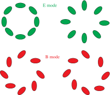
Figure 9: Illustration of shape distortion patterns from $E$-mode and $B$-mode fields. Image reproduced with permission from Van Waerbeke and Mellier (2003).

Figure 9 illustrates characteristic distortion patterns from $E$-mode (curl-free) and $B$-mode (divergence-free) fields. Weak lensing only produces curl-free $E$-mode signals, so that the presence of divergence-free $B$ modes can be used as a null test for systematic effects. In the weak-lensing regime, a tangential $E$-mode pattern is produced by a positive mass overdensity (e.g., halos), while a radial $E$-mode pattern is produced by a negative mass overdensity (e.g., cosmic voids).

Now we turn to the issue of $E$/$B$-mode reconstructions from the spin-2 shear field. Rewriting Eq. (58) in terms of the complex shear $\gamma$, we find:

$$\triangle\kappa_{E} =\Re\left(2\hat{\cal D}^{*}\gamma\right),$$ (59)

$$\triangle\kappa_{B} =\Im\left(2\hat{\cal D}^{*}\gamma\right),$$

where $\Re(Z)$ and $\Im(Z)$ denote the real part and the imaginary part of a complex variable $Z$, respectively. Defining $\kappa\equiv\kappa_{E}+i\kappa_{B}$, we see that the first of Eq. (59) is identical to the mass inversion formula (Eq. (42)). The $B$-mode convergence $\kappa_{B}$ can thus be simply obtained as the imaginary part of Eq. (44), which is expected to vanish for a purely weak-lensing signal. Moreover, the second of Eq. (59) indicates that the transformation $\gamma^{\prime}(\mbox{\boldmath$\theta$})=i\gamma(\mbox{\boldmath$\theta$})$ ($\gamma_{1}^{\prime}=-\gamma_{2},\gamma_{2}^{\prime}=\gamma_{1}$) is equivalent to an interchange operation of the $E$ and $B$ modes of the original maps by $\kappa_{E}^{\prime}(\mbox{\boldmath$\theta$})=-\kappa_{B}(\mbox{\boldmath$\theta$})$ and $\kappa^{\prime}_{B}(\mbox{\boldmath$\theta$})=\kappa_{E}(\mbox{\boldmath$\theta$})$. Since $\gamma$ is a spin-2 field that transforms as $\gamma^{\prime}=\gamma e^{2i\varphi}$, this operation is also equivalent to a rotation of each ellipticity by $\pi/4$ with each position vector fixed.

Note that gravitational lensing can induce $B$ modes, for example, when multiple deflections of light are involved (Sect. 2.5). However, these $B$ modes can be generated at higher orders and the $B$-mode contributions coming from multiple deflections are suppressed by a large factor compared to the $E$-mode contributions (see, e.g., Krause and Hirata, 2010). In real observations, intrinsic ellipticities of background galaxies also contribute to weak-lensing shear estimates. Assuming that intrinsic ellipticities have random orientations in projection space, such an isotropic ellipticity distribution will yield statistically identical contributions to the $E$ and $B$ modes. Therefore, the $B$-mode signal provides a useful null test for systematic effects in weak-lensing observations (Fig. 9).

3.3 Flexion

Flexion is introduced as the next higher-order lensing effects responsible for an arc-like and weakly skewed appearance of lensed galaxies (Goldberg and Bacon, 2005; Bacon et al., 2006) observed in a regime between weak and strong lensing (i.e., a nonlinear but subcritical regime). Such higher-order lensing effects occur when $\kappa(\mbox{\boldmath$\theta$})$ and $\gamma(\mbox{\boldmath$\theta$})$ are not spatially constant across a source galaxy image. By taking higher-order derivatives of the lensing potential $\psi(\mbox{\boldmath$\theta$})$, we can work with higher-order transformations of galaxy shapes by weak lensing (e.g., Massey et al., 2007b; Okura et al., 2007, 2008; Goldberg and Leonard, 2007; Schneider and Er, 2008; Viola et al., 2012).

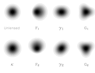
Figure 10: Weak-lensing distortions with different spin values increasing from left to right. The convergence $\kappa$ is a spin-0 quantity, the first flexion $F=F_{1}+iF_{2}$ is spin-1, the shear $\gamma=\gamma_{1}+i\gamma_{2}$ is spin-2, and the second flexion $G=G_{1}+iG_{2}$ is spin-3. Image reproduced with permission from Bacon et al. (2006), copyright by the authors.

The third-order derivatives of $\psi(\mbox{\boldmath$\theta$})$ can be combined to form a pair of complex flexion fields as (Bacon et al., 2006):

$$F :=F_{1}+i{F}_{2}=\frac{1}{2}\partial\partial\partial^{*}\psi=\partial\kappa,$$ (60)

$$G :=G_{1}+i{G}_{2}=\frac{1}{2}\partial\partial\partial\psi=\partial\gamma.$$

The first flexion ${F}$ has spin-1 and the second flexion ${G}$ has spin-3. The two complex flexion fields satisfy the following consistency relation:

$$\partial^{*}\partial G(\mbox{\boldmath$\theta$})=\partial\partial F(\mbox{\boldmath$\theta$}).$$ (61)

Figure 10 illustrates the characteristic weak-lensing distortions with different spin values for an intrinsically circular Gaussian source (Bacon et al., 2006).

If the angular size of an image is small compared to the characteristic scale over which $\psi(\mbox{\boldmath$\theta$})$ varies, we can locally expand Eq. (13) to the next higher order as:

$$\delta\beta_{i}={\cal A}_{ij}\delta\theta_{j}+\frac{1}{2}{\cal A}_{ij,k}\delta\theta_{j}\delta\theta_{k}+O(\delta\theta^{3}),$$ (62)

where ${\cal A}_{ij,k}=-\psi_{,ijk}$ ($i,j,k=1,2$). The ${\cal A}_{ij,k}$ matrix can be expressed with a sum of two terms:

$${\cal A}_{ij,k}={F}_{ijk}+{G}_{ijk},$$ (63)

with the spin-1 part ${F}_{ijk}$ and the spin-3 part ${G}_{ijk}$ defined by:

$${F}_{ij1}=-\frac{1}{2}\left(\begin{array}[]{@{\,}cc@{\,}}3{F}_{1}&{F}_{2}\\ {F}_{2}&{F}_{1}\end{array}\right) \ \ {F}_{ij2}=-\frac{1}{2}\left(\begin{array}[]{@{\,}cc@{\,}}{F}_{2}&{F}_{1}\\ {F}_{1}&3{F}_{2}\end{array}\right),$$ , (68)

$${G}_{ij1}=-\frac{1}{2}\left(\begin{array}[]{@{\,}cc@{\,}}{G}_{1}&{G}_{2}\\ {G}_{2}&-{G}_{1}\end{array}\right) \ \ {G}_{ij2}=-\frac{1}{2}\left(\begin{array}[]{@{\,}cc@{\,}}{G}_{2}&-{G}_{1}\\ -{G}_{1}&-{G}_{2}\end{array}\right).$$ , (73)

Flexion has a dimension of inverse (angular) length, so that the flexion effects depend on the angular size of the source image. That is, the smaller the source image, the larger the amplitude of intrinsic flexion contributions (Okura et al., 2008). The shape quantities affected by the first flexion ${F}$ alone have spin-1 properties, while those by the second flexion ${G}$ alone have spin-3 properties.

Note that, as in the case of the spin-2 shear field, what is directly observable from higher-order image distortions are the reduced flexion effects, $F/(1-\kappa)$ and $G/(1-\kappa)$ (Okura et al., 2007, 2008; Goldberg and Leonard, 2007; Schneider and Er, 2008), a consequence of the mass-sheet degeneracy.

From Eq. (60), the inversion equations from flexion to $\kappa$ can be obtained as follows (Bacon et al., 2006):

$$(\kappa+iB)_{F} = \triangle^{-1}\partial^{*}{F},$$ (74)

$$(\kappa+iB)_{G} = \triangle^{-2}\partial^{*}\partial^{*}\partial^{*}{G},$$ (75)

where the complex part $iB$ describes the $B$-mode component that can be used to assess the noise properties of weak-lensing data (e.g., Okura et al., 2008). An explicit representation for the inversion equations is obtained in Fourier space as:

$$\widehat{\kappa}_{F}(\mbox{\boldmath$k$}) =-i\frac{k_{1}\widehat{F}_{1}+k_{2}\widehat{F}_{2}}{k_{1}^{2}+k_{2}^{2}},$$ (76)

$$\widehat{\kappa}_{G}(\mbox{\boldmath$k$}) =-i\frac{\widehat{G}_{1}(k_{1}^{3}-3k_{1}k_{2}^{2})+\widehat{G}_{2}(3k_{1}^{2}k_{2}-k_{2}^{3})}{(k_{1}^{2}+k_{2}^{2})^{2}},$$

for $\mbox{\boldmath$k$}\neq 0$.

In principle one can combine independent mass reconstructions $\widehat{\kappa}_{a}(\mbox{\boldmath$k$})$ $(a=\gamma,{F},{G})$ linearly in Fourier space to improve the statistical significance with minimum noise variance weighting as (Okura et al., 2007):

$$\widehat{\kappa}(\mbox{\boldmath$k$})=\frac{\sum_{a}\widehat{W}_{\kappa|a}(\mbox{\boldmath$k$})\widehat{\kappa}_{a}(\mbox{\boldmath$k$})}{\sum_{a}\widehat{W}_{\kappa|a}(\mbox{\boldmath$k$})},$$ (77)

where $\widehat{W}_{\kappa|a}(\mbox{\boldmath$k$})=1/P^{(N)}_{\kappa a}(\mbox{\boldmath$k$})$ with $P^{(N)}_{\kappa|a}(\mbox{\boldmath$k$})$ the two-dimensional noise power spectrum of $\kappa$ reconstructed using the observable $a$:

$$P^{(N)}_{\kappa|\gamma}(\mbox{\boldmath$k$}) =\frac{P_{\gamma}^{(N)}(\mbox{\boldmath$k$})}{2}=\frac{\sigma^{2}_{\gamma}}{2n_{\gamma}},$$ (78)

$$P^{(N)}_{\kappa|F}(\mbox{\boldmath$k$}) =\frac{P^{(N)}_{F}(\mbox{\boldmath$k$})}{2k^{2}}=\frac{\sigma^{2}_{F}}{2n_{F}\mbox{\boldmath$k$}^{2}},$$

$$P^{(N)}_{\kappa|G}(\mbox{\boldmath$k$}) =\frac{P^{(N)}_{G}(\mbox{\boldmath$k$})}{2k^{2}}=\frac{\sigma^{2}_{G}}{2n_{G}\mbox{\boldmath$k$}^{2}},$$

with $P^{(N)}_{a}(\mbox{\boldmath$k$})$ the shot noise power, $\sigma_{a}$ the shape noise dispersion, and $n_{a}$ the mean surface number density of background source galaxies, for the observable $a$ ($a=\gamma,F,G$). Assuming that errors in $\widehat{\kappa}_{a}(\mbox{\boldmath$k$})$ between different observables are independent, the noise power spectrum for the estimator (Eq. (77)) is obtained as (Okura et al., 2007):

$$P^{(N)}_{\kappa}(\mbox{\boldmath$k$})=\frac{1}{\sum_{a}\widehat{W}_{a}(\mbox{\boldmath$k$})}=\frac{1}{\sum_{a}1/P^{(N)}_{\kappa|a}(\mbox{\boldmath$k$})}.$$ (79)

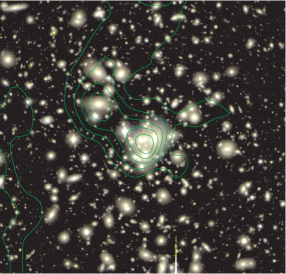
Figure 11: Mass contours of the rich cluster Abell 1689 ($z_{l}=0.183$) reconstructed from spin-1 flexion measurements based on Subaru Suprime-Cam observations, superposed on the Suprime-Cam $Vi^{\prime}$ color image. The contours are spaced in units of $1\sigma$ reconstruction error estimated from the rms of the $B$-mode reconstruction. The field size is $4^{\prime}\times 4^{\prime}$. North is to the top and east to the left. Image reproduced with permission from Okura et al. (2008), copyright by AAS.

Figure 11 shows the $\kappa$ field in the central region of the rich cluster Abell 1689 ($z_{l}=0.183$) reconstructed from the spin-1 flexion alone (Okura et al., 2008) measured with Subaru Suprime-Cam data. Okura et al. (2008) used measurements of higher-order lensing image characteristics (HOLICs) introduced by Okura et al. (2007). Their analysis accounted for the effect of the weight function used for calculating noisy shape moments, as well as for higher-order PSF effects. One can employ the assumption of random orientations for intrinsic HOLICs of background galaxies to obtain a direct estimate of flexion, in a similar manner to the usual prescription for weak shear lensing. Okura et al. (2008) utilized the Fourier-space relation (Eq. (76)) between $F(\mbox{\boldmath$\theta$})$ and $\kappa(\mbox{\boldmath$\theta$})$ with the linear weak-lensing approximation. The $B$-mode convergence field was used to monitor the reconstruction error in the $\kappa$ map. The reconstructed $\kappa$ map exhibits a bimodal feature in the central region of the cluster. The pronounced main peak is associated with the brightest cluster galaxy (BCG) and central cluster members, while the secondary mass peak is associated with a local concentration of bright galaxies.

Note that, as discussed in Viola et al. (2012), there is a cross-talk between shear and flexion arising from shear–flexion coupling terms, which makes quantitative measurements of flexion challenging.

3.4 Shear observables

Since the pioneering work of Kaiser et al. (1995), numerous methods have been proposed and implemented in the literature to accurately extract the lensing signal from noisy pixelized images of background galaxies (e.g., Kuijken, 1999; Bridle et al., 2002; Bernstein and Jarvis, 2002; Refregier, 2003; Hirata and Seljak, 2003; Miller et al., 2007). On the other hand, considerable progress has been made in understanding and controlling systematic biases in noisy shear estimates by relying on realistic galaxy image simulations (e.g., Heymans et al., 2006; Massey et al., 2007a; Refregier et al., 2012; Kacprzak et al., 2012; Mandelbaum et al., 2014, 2015, 2018a).

Here we will review the basic idea and essential aspects of the moment-based KSB formalism. We refer the reader to Mandelbaum (2018) for a recent exhaustive review on the subject.

3.4.1 Ellipticity transformation by weak lensing

In a moment-based approach to weak-lensing shape measurements, we use quadrupole moments $Q_{ij}$ ($i,j=1,2$) of the surface brightness distribution $I(\mbox{\boldmath$\theta$})$ of background galaxy images to quantify the shape of the images as (Kaiser et al., 1995):

$$Q_{ij}\equiv\frac{\int\!d^{2}\theta\,q_{I}[I(\mbox{\boldmath$\theta$})]\Delta\theta_{i}\Delta\theta_{j}}{\int d^{2}\theta\,q_{I}[I(\mbox{\boldmath$\theta$})]},$$ (80)

where $q_{I}[I(\mbox{\boldmath$\theta$})]$ is a weight function and $\Delta\theta_{i}=\theta_{i}-\overline{\theta}_{i}$ denotes the offset vector from the image centroid. Here we assume that the weight $q_{I}$ does not explicitly depend on $\theta$ but is set by the local value of the brightness $I(\mbox{\boldmath$\theta$})$ (Bartelmann and Schneider, 2001). The trace of $Q_{ij}$ describes the angular size of the image, while the traceless part describes the shape and orientation of the image. With the quadrupole moments $Q_{ij}$, we define the complex ellipticity $e=e_{1}+ie_{2}$ as:

$$e\equiv\frac{Q_{11}-Q_{22}+2iQ_{12}}{Q_{11}+Q_{22}}.$$ (81)

For an ellipse with a minor-to-major axis ratio of $q$ $(\leqslant 1)$, $|e|=(1-q^{2})/(1+q^{2})$.

The spin-2 ellipticity $e$ (Eq. (81)) transforms under the lens mapping as:

$$e^{(s)}=\frac{e-2g+e^{*}g^{2}}{1+|g|^{2}-2\Re(e^{*}g)},$$ (82)

where $e^{(s)}$ is the unlensed intrinsic ellipticity and $g=\gamma/(1-\kappa)$ is the spin-2 reduced shear. Since $e$ is a nonzero spin quantity with a direction dependence, the expectation value of the intrinsic source ellipticity $e^{(s)}$ is assumed to vanish, i.e., ${\cal E}(e^{(s)})=0$, where ${\cal E}(X)$ denotes the expectation value of $X$. Schneider and Seitz (1995) showed that Eq. (82) with the condition ${\cal E}(e^{(s)})=0$ is equivalent to:

$$0=\sum_{n}w_{n}\frac{e_{n}-\delta_{g}}{1-\Re(e^{*}_{n}\delta_{g})},$$ (83)

where $e_{n}$ is the image ellipticity for the $n$th object, $w_{n}$ is a statistical weight for the $n$th object, and $\delta_{g}$ is the spin-2 complex distortion (Schneider and Seitz, 1995):

$$\delta_{g}\equiv\frac{2g}{1+|g|^{2}}.$$ (84)

Note that the complex distortion $\delta_{g}$ is invariant under the transformation $g\to 1/g^{*}$.

For an intrinsically circular source with $e^{(s)}=0$, we have:

$$e=\delta_{g}=\frac{2g}{1+|g|^{2}}.$$ (85)

On the other hand, in the weak-lensing limit ($|\kappa|,|\gamma|\ll 1$), Eq. (82) reduces to $e^{(s)}\simeq e-2g\simeq e-2\gamma$. Assuming random orientations of source galaxies, we average observed ellipticities over a local ensemble of source galaxies to obtain:

$$\gamma\simeq g\simeq\frac{{\cal E}(e)}{2}.$$ (86)

For an input signal of $g=0.1$, Eq. (85) yields $e\approx 0.198$. Hence, the weak-lensing approximation (Eq. (86)) gives a reduced-shear estimate of $g^{\mathrm{(est)}}\approx 0.099$, corresponding to a negative bias of $1\%$. For $g=0.2$ in the mildly nonlinear regime, Eq. (86) gives $g^{\mathrm{(est)}}\approx 0.192$, corresponding to a negative bias of $4\%$.

In real observations, the reduced shear $g$ may be estimated from a local ensemble average of background galaxies as $\langle g\rangle\simeq\langle e\rangle/2$. The statistical uncertainty in the reduced-shear estimate $\langle g\rangle$ decreases with increasing the number of background galaxies $N$ (see Sect. 4.2 for more details) as $\propto\sigma/\sqrt{N}$, with $\sigma$ the dispersion of background image ellipticities (dominated by the intrinsic shape noise). Weak-lensing analysis thus requires a large number of background galaxies to increase the statistical significance of the shear measurements.

3.4.2 The KSB algorithm: a moment-based approach

For a practical application of weak shear lensing, we must account for various observational and instrumental effects, such as the impact of noise on the galaxy shape measurement (both statistical and systematic uncertainties), the isotropic smearing component of the PSF, and the effect of instrumental PSF anisotropy. Therefore, one cannot simply use Eq. (86) to measure the shear signal from observational data.

A more robust estimate of the shape moments (Eq. (80)) is obtained by using a weight function $W(|\mbox{\boldmath$\theta$}|)$ that depends explicitly on the separation $|\mbox{\boldmath$\theta$}|$ from the image centroid. In the KSB approach, a circular Gaussian that is matched to the size of each object is used as a weight function (Kaiser et al., 1995). The quadrupole moments obtained with such a weight function $W(|\mbox{\boldmath$\theta$}|)$ suffer from an additional smearing and do not obey the transformation law (Eq. (82)). Therefore, the expectation value ${\cal E}(e)$ of the image ellipticity is different from the distortion $\delta_{g}=2g/(1+|g|^{2})$ (see Eq. (85)).

The KSB formalism (Kaiser et al., 1995; Hoekstra et al., 1998) accounts explicitly for the Gaussian weight function used for measuring noisy shape moments, the effect of spin-2 PSF anisotropy, and the effect of isotropic PSF smearing. The KSB formalism and its variants assume that the PSF can be described as an isotropic function convolved with a small anisotropic kernel. In the limit of linear response to lensing and instrumental anisotropies, KSB derived the transformation law between intrinsic (unlensed) and observed (lensed) complex ellipticities, $e^{(s)}$ and $e$, respectively. The linear transformation between intrinsic and observed complex ellipticities can be formally expressed as (Kaiser et al., 1995; Hoekstra et al., 1998; Bartelmann and Schneider, 2001):

$$e_{i}=e_{i}^{(s)}+\left(C^{g}\right)_{ij}g_{j}+\left(C^{q}\right)_{ij}q_{j}\ \ (i,j=1,2),$$ (87)

where $q_{i}$ denotes the spin-2 PSF anisotropy kernel, $(C^{q})_{ij}$ is a linear response matrix for the PSF anisotropy $q_{i}$, $(C^{g})_{ij}$ is a linear response matrix for the reduced shear $g_{i}$. The PSF anisotropy kernel and the response matrices can be calculated from observable weighted shape moments of galaxies and stellar objects (Kaiser et al., 1995; Bartelmann and Schneider, 2001; Erben et al., 2001). In real observations, the PSF anisotropy kernel $q(\mbox{\boldmath$\theta$})$ can be estimated from image ellipticities $e^{*}$ observed for a sample of foreground stars for which $e^{(s)}$ and $g$ vanish, so that $q_{i}(\mbox{\boldmath$\theta$})=(C^{q})^{-1}_{ij}e^{*}_{j}$.

Assuming that the expectation value of the intrinsic source ellipticity vanishes ${\cal E}[e^{(s)}]=0$, we find the following linear relation between the reduced shear and the ensemble-averaged image ellipticity:

$$g_{i}={\cal E}\left[\left(C^{g}\right)^{-1}_{ij}(e-C^{q}q)_{j}\right]\ \ \ (i,j=1,2).$$ (88)

In the KSB formalism, the shear response matrix $C^{g}$ is denoted as $P^{g}$ (or $P^{\gamma}$) and dubbed pre-seeing shear polarizability. Similarly, $C^{q}$ is denoted as $P^{\mathrm{sm}}$ and dubbed smear polarisability.

A careful calibration of the signal response $P^{g}$ is essential for any weak shear lensing analysis that relies on accurate shape measurements from galaxy images (see Mandelbaum, 2018). The levels of shear calibration bias are often quantified in terms of a multiplicative bias factor $m$ and an additive calibration offset $c$ through the following relation between the true input shear signal, $g^{\mathrm{true}}$, and the recovered signal, $g^{\mathrm{obs}}$ (Heymans et al., 2006; Massey et al., 2007a; Mandelbaum et al., 2014):

$$g_{i}^{\mathrm{obs}}=(1+m_{i})g_{i}^{\mathrm{true}}+c_{i}\ \ (i=1,2),$$ (89)

The original KSB formalism, when applied to noisy observations, is known to suffer from systematic biases that depend primarily on the size and the detection signal-to-noise ratio (S/N) of galaxy images (e.g., Erben et al., 2001; Refregier et al., 2012). Different variants of the Kaiser et al. (1995) method (KSB+) have been developed and implemented in the literature primarily to study mass distributions of high-mass galaxy clusters (e.g., Hoekstra et al., 1998, 2015; Clowe et al., 2004; Umetsu et al., 2010, 2014; Oguri et al., 2012; von der Linden et al., 2014a; Okabe and Smith, 2016; Schrabback et al., 2018). Note that KSB+ pipelines calibrated against realistic image simulations of crowded fields can achieve a $\sim 2\%$ shear calibration accuracy even in the cluster lensing regime (e.g., Herbonnet et al., 2020; Hernández-Martín et al., 2020).

3.5 Tangential- and cross-shear components

As we have seen in Sect. 3.1, the spin-2 shear components $\gamma_{1}$ and $\gamma_{2}$ are coordinate dependent, defined relative to a reference Cartesian coordinate frame (chosen by the observer). It is useful to consider components of the shear that are coordinate independent with respect to a certain reference point, such as the cluster center.

We define a polar coordinate system ($\vartheta,\varphi$) centered on an arbitrary point $\mbox{\boldmath$\theta$}_{\mathrm{c}}$ on the sky, such that $\mbox{\boldmath$\theta$}=(\vartheta\cos\varphi,\vartheta\sin\varphi)+\mbox{\boldmath$\theta$}_{\mathrm{c}}$. The convergence $\overline{\kappa}(\vartheta)$ averaged within a circle of radius $\vartheta$ about $\mbox{\boldmath$\theta$}_{\mathrm{c}}$ is then expressed as:

$$\overline{\kappa}(\vartheta) :=\frac{2}{\vartheta^{2}}\int_{0}^{\vartheta}\!d\vartheta^{\prime}\,\vartheta^{\prime}\kappa(\vartheta^{\prime})\equiv\frac{\overline{\Sigma}(\vartheta)}{\Sigma_{\mathrm{cr}}},$$ (90)

$$\kappa(\vartheta) :=\oint\!\frac{d\varphi}{2\pi}\,\kappa(\vartheta,\varphi)\equiv\frac{\Sigma(\vartheta)}{\Sigma_{\mathrm{cr}}},$$

where $\overline{\Sigma}(\vartheta)$ is the surface mass density averaged within a circle of radius $\vartheta$ about $\mbox{\boldmath$\theta$}_{\mathrm{c}}$ and $\Sigma(\vartheta)$ is the surface mass density averaged over a circle of radius $\vartheta$ about $\mbox{\boldmath$\theta$}_{\mathrm{c}}$. The reference point $\mbox{\boldmath$\theta$}_{\mathrm{c}}$ can be taken to be the cluster center, which can be determined from symmetry of the strong-lensing pattern, the X-ray centroid position, or the BCG position.

Let us introduce the tangential and $45^{\circ}$-rotated cross shear components, $\gamma_{+}(\mbox{\boldmath$\theta$})$ and $\gamma_{\times}(\mbox{\boldmath$\theta$})$, respectively, defined relative to the position $\mbox{\boldmath$\theta$}_{\mathrm{c}}$ as:

$$\gamma_{+}(\mbox{\boldmath$\theta$}) =-\gamma_{1}(\mbox{\boldmath$\theta$})\cos(2\varphi)-\gamma_{2}(\mbox{\boldmath$\theta$})\sin(2\varphi),$$ (91)

$$\gamma_{\times}(\mbox{\boldmath$\theta$}) =+\gamma_{1}(\mbox{\boldmath$\theta$})\sin(2\varphi)-\gamma_{2}(\mbox{\boldmath$\theta$})\cos(2\varphi),$$

which are directly observable in the weak-lensing limit where $|\kappa|,|\gamma|\ll 1$ (see Sect. 3.4). Using the two-dimensional version of Gauss’ theorem, we find the following identity for an arbitrary choice of $\mbox{\boldmath$\theta$}_{\mathrm{c}}$ (Kaiser, 1995):

$$\gamma_{+}(\vartheta) :=\oint\!\frac{d\varphi}{2\pi}\,\gamma_{+}(\vartheta,\varphi)=\overline{\kappa}(\vartheta)-\kappa(\vartheta)\equiv\frac{\Delta\Sigma(\vartheta)}{\Sigma_{\mathrm{cr}}},$$ (92)

$$\gamma_{\times}(\vartheta) :=\oint\!\frac{d\varphi}{2\pi}\,\gamma_{\times}(\vartheta,\varphi)=0,$$

where we have defined the excess surface mass density $\Delta\Sigma(\vartheta)$ around $\mbox{\boldmath$\theta$}_{\mathrm{c}}$ as a function of $\vartheta$ by (Miralda-Escude, 1991):

$$\Delta\Sigma(\vartheta)=\overline{\Sigma}(\vartheta)-\Sigma(\vartheta).$$ (93)

From Eqs. (90) and (92), we find:

$$\frac{d\overline{\kappa}(\vartheta)}{d\ln\vartheta}=-2\gamma_{+}(\vartheta).$$ (94)

Equation (92) shows that, given an arbitrary circular loop of radius $\vartheta$ around the chosen center $\mbox{\boldmath$\theta$}_{\mathrm{c}}$, the tangential and cross shear components averaged around the loop extract $E$-mode and $B$-mode distortion patterns (Sect. 3.2).

An important implication of the first of Eq. (92) is that, with tangential shear measurements from individual source galaxies (see Sect. 3.4), one can directly determine the azimuthally averaged $\Delta\Sigma(\vartheta)$ profile around lenses in the weak-lensing regime, even if the mass distribution $\Sigma(\mbox{\boldmath$\theta$})$ is not axis-symmetric around $\mbox{\boldmath$\theta$}_{\mathrm{c}}$. Moreover, the second of Eq. (92) tells us that the azimuthally averaged $\times$ component, or the $B$-mode signal, is expected to be statistically consistent with zero if the signal is due to weak lensing. Therefore, a measurement of the $B$-mode signal $\langle g_{\times}(\vartheta)\rangle$ provides a useful null test against systematic errors.

3.6 Reduced tangential shear

3.6.1 Azimuthally averaged reduced tangential shear

The reduced tangential shear $g_{+}(\vartheta)$ averaged over a circle of radius $\vartheta$ about an arbitrary reference point $\mbox{\boldmath$\theta$}_{\mathrm{c}}$ is expressed as:

$$g_{+}(\vartheta) :=\oint\!\frac{d\varphi}{2\pi}\,g_{+}(\vartheta,\varphi)=\oint\!\frac{d\varphi}{2\pi}\,\frac{\gamma_{+}(\vartheta,\varphi)}{1-\kappa(\vartheta,\varphi)}.$$ (95)

If the projected mass distribution around a cluster has quasi-circular symmetry (e.g., elliptical symmetry), then the azimuthally averaged reduced tangential shear $\langle g_{+}(\vartheta)\rangle$ around the cluster center can be interpreted as:

$$g_{+}(\vartheta)\simeq\frac{\gamma_{+}(\vartheta)}{1-\kappa(\vartheta)},$$ (96)

where $\gamma_{+}(\vartheta)$ and $\kappa(\vartheta)$ are the tangential shear and the convergence, respectively, averaged over a circle of radius $\vartheta$ about $\mbox{\boldmath$\theta$}_{\mathrm{c}}$.

According to $N$-body simulations in hierarchical $\mathrm{\Lambda}$CDM models of cosmic structure formation, dark matter halos exhibit aspherical mass distributions that can be well approximated by triaxial mass models (e.g., Jing and Suto, 2002; Limousin et al., 2013; Despali et al., 2014). Since triaxial halos have elliptical isodensity contours in projection on the sky (Stark, 1977), Eq. (96) can give a good approximation to describe the weak-lensing signal for regular clusters with a modest degree of perturbation. However, the approximation is likely to break down for merging and interacting lenses having complex, multimodal mass distributions. To properly model the weak-lensing signal in such a complex merging system, one needs to directly model the two-dimensional reduced-shear field $(g_{1}(\mbox{\boldmath$\theta$}),g_{2}(\mbox{\boldmath$\theta$}))$ with a lens model consisting of multi-component halos (e.g., Watanabe et al., 2011; Okabe et al., 2011; Medezinski et al., 2013). Alternatively, one may attempt to reconstruct the convergence field $\kappa(\mbox{\boldmath$\theta$})$ in a free-form manner from the observed reduced shear field, with additional constraints or assumptions to break the mass-sheet degeneracy (e.g., Jee et al., 2005; Bradač et al., 2006; Merten et al., 2009; Jauzac et al., 2012; Umetsu et al., 2015; Tam et al., 2020).

On the other hand, for a statistical ensemble of galaxy clusters, the average mass distribution around their centers tends to be spherically symmetric if the assumption of statistical isotropy holds (e.g., Okabe et al., 2013). Hence, the stacked weak-lensing signal for a statistical ensemble of clusters can be interpreted using Eq. (96). For more details, see Sects. 3.6.4 and 4.5.

3.6.2 Source-averaged reduced tangential shear

With the assumption of quasi-circular symmetry in the projected mass distribution around clusters (see Eq. (96)), let us consider the nonlinear effects on the source-averaged cluster lensing profiles. The reduced tangential shear for a given lens–source pair is written as:

$$g_{+}(\vartheta|z_{l},z_{s}) =\Delta\Sigma(\vartheta)\sum_{n=0}^{\infty}\left[\Sigma_{\mathrm{cr}}^{-1}(z_{l},z_{s})\right]^{n+1}\Sigma^{n}(\vartheta).$$ (97)

To begin with, let us consider the expectation value for the reduced tangential shear averaged over an ensemble of source galaxies. For a given cluster, the source-averaged reduced tangential shear is expressed as:

$$\langle g_{+}(\vartheta|z_{l})\rangle=\Delta\Sigma\left[\langle\Sigma_{\mathrm{cr},l}^{-1}\rangle+\langle\Sigma_{\mathrm{cr},l}^{-2}\rangle\Sigma+\langle\Sigma_{\mathrm{cr},l}^{-3}\rangle\Sigma^{2}+\cdots\right],$$ (98)

where $\langle\cdots\rangle$ denotes the averaging over all sources, defined such that:

$$\langle\Sigma_{\mathrm{cr},l}^{-n}\rangle=\left(\sum_{s}w_{s}\Sigma_{\mathrm{cr},ls}^{-n}\right)\left(\sum_{s}w_{s}\right)^{-1},$$ (99)

where the index $s$ runs over all source galaxies around the lens ($l$) and $w_{s}$ is a statistical weight for each source galaxy. An optimal choice for the statistical weight is $w_{s}=1/\sigma_{g_{+},s}^{2}$, with $\sigma_{g_{+},s}$ the statistical uncertainty of $g_{+}(\vartheta|z_{l},z_{s})$ estimated for each source galaxy. Note that this choice for the weight assumes that $\sigma_{g_{+},s}$ is independent of the lensing shear signal (see Schneider and Seitz, 1995; Seitz and Schneider, 1995). In the continuous limit, Eq. (99) is written as:

$$\langle\Sigma_{\mathrm{cr},l}^{-n}\rangle=\left[\int_{0}^{\infty}\!dz\,\frac{dN(z)}{dz}w(z)\Sigma_{\mathrm{cr}}^{-n}(z_{l},z)\right]\left[\int_{0}^{\infty}\!dz\,\frac{dN(z)}{dz}w(z)\right]^{-1},$$ (100)

with $dN(z)/dz$ the redshift distribution function of the source sample and $w(z)$ a statistical weight function. For a given cluster lens, $\Sigma_{\mathrm{cr}}^{-1}(z_{l},z_{s})\propto D_{ls}/D_{s}$, so that $\langle\Sigma_{\mathrm{cr},l}^{-n}\rangle\propto\langle(D_{ls}/D_{s})^{n}\rangle$.

In the weak-lensing limit, Eq. (98) gives $\langle g_{+}\rangle\simeq\langle\gamma_{+}\rangle$. The next order of approximation is given by (Seitz and Schneider, 1997):

$$\langle g_{+}\rangle \simeq\frac{\langle\gamma_{+}\rangle}{1-f_{l}\langle\kappa\rangle},$$ (101)

$$f_{l} =\frac{\langle\Sigma_{\mathrm{cr},l}^{-2}\rangle}{\langle\Sigma_{\mathrm{cr},l}^{-1}\rangle^{2}}.$$

From Eq. (101), we see that an interpretation of the averaged weak-lensing signal $\langle g_{+}(\vartheta|z_{l})\rangle$ does not require knowledge of individual source redshifts. Instead, it requires ensemble information regarding the statistical redshift distribution $dN(z)/dz$ of background source galaxies used for weak-lensing measurements.

For a lens at sufficiently low redshift (see Sect. 2.6.5), $f_{l}\approx 1$, thus leading to the single source-plane approximation: $\langle g_{+}\rangle\simeq\langle\gamma_{+}\rangle/(1-\langle\kappa\rangle)$. The level of bias introduced by this approximation is $\Delta\langle g_{+}\rangle/\langle g_{+}\rangle\simeq(f_{l}-1)\langle\kappa\rangle$. In typical ground-based deep observations of $z_{l}\sim 0.4$ clusters, $\Delta f_{l}=f_{l}-1$ is found to be of the order of several percent (Umetsu et al., 2014), so that the relative error $\Delta\langle g_{+}\rangle/\langle g_{+}\rangle$ is negligibly small in the mildly nonlinear regime of cluster lensing.

3.6.3 Source-averaged excess surface mass density

Next, let us consider the following estimator for the excess surface mass density $\Delta\Sigma(\vartheta)$ for a given lens–source pair:

$$\Delta\Sigma_{+}(\vartheta|z_{l},z_{s}):=\Sigma_{\mathrm{cr}}(z_{l},z_{s})g_{+}(\vartheta|z_{l},z_{s}).$$ (102)

This assumes that an estimate of $\Sigma_{\mathrm{cr}}^{-1}(z_{l},z_{s})$ for each individual source galaxy is available, for example, from photometric-redshift (photo-$z$) measurements. This estimator is widely used in recent cluster weak-lensing studies thanks to the availability of multi-band imaging data and the advances in photo-$z$ techniques (see Sect. 4.1).

In real observations, if the photo-$z$ probability distribution function (PDF), $P_{s}(z)$, is available for individual source galaxies ($s$), one can calculate:

$$\Sigma^{-1}_{\mathrm{cr},ls}\equiv\left[\int\!dz\,P_{s}(z)\Sigma_{\mathrm{cr}}^{-1}(z_{l},z)\right]\left[\int\!dz\,P_{s}(z)\right]^{-1}$$ (103)

averaged over the PDF for each source galaxy. Similarly to Eq. (98), $\Delta\Sigma_{+}(\vartheta|z_{l},z_{s})$ averaged over all sources is expressed as:

$$\langle\Delta\Sigma_{+}\rangle=\Delta\Sigma\left[1+\langle\Sigma_{\mathrm{cr},l}^{-1}\rangle\Sigma+\langle\Sigma_{\mathrm{cr},l}^{-2}\rangle\Sigma^{2}+\cdots\right]$$ (104)

with

$$\langle\Sigma_{\mathrm{cr},l}^{-n}\rangle=\left(\sum_{s}w_{ls}\Sigma_{\mathrm{cr},ls}^{-n}\right)\left(\sum_{s}w_{ls}\right)^{-1},$$ (105)

where the index $s$ runs over all source galaxies around the lens ($l$) and $w_{ls}$ is a statistical weight for each source galaxy. An optimal choice for the statistical weight is:

$$w_{ls}=\Sigma_{\mathrm{cr},ls}^{-2}/\sigma_{g_{+},s}^{2},$$ (106)

where $\sigma_{g_{+},s}$ is the statistical uncertainty of $g_{+}(\vartheta|z_{l},z_{s})$ estimated for each source galaxy (Sect. 3.6.2).

In the weak-lensing limit, we thus have $\langle\Delta\Sigma_{+}\rangle\simeq\Delta\Sigma$. The next order of approximation is:

$$\langle\Delta\Sigma_{+}\rangle\simeq\frac{\Delta\Sigma}{1-\langle\Sigma_{\mathrm{cr},l}^{-1}\rangle\Sigma}.$$ (107)

3.6.4 Lens–source-averaged excess surface mass density

Finally, we consider an ensemble of galaxy clusters. Now, let $\Delta\Sigma$ be the ensemble mass distribution of these clusters. Then, $\Delta\Sigma_{+}$ averaged over all lens–source ($ls$) pairs is expressed as (Johnston et al., 2007):

$$\langle\!\langle\Delta\Sigma_{+}\rangle\!\rangle=\Delta\Sigma\left[1+\langle\!\langle\Sigma_{\mathrm{cr}}^{-1}\rangle\!\rangle\Sigma+\langle\!\langle\Sigma_{\mathrm{cr}}^{-2}\rangle\!\rangle\Sigma^{2}+\cdots\right]$$ (108)

with

$$\langle\!\langle\Sigma_{\mathrm{cr}}^{-n}\rangle\!\rangle=\left(\sum_{l,s}w_{ls}\Sigma_{\mathrm{cr},ls}^{-n}\right)\left(\sum_{l,s}w_{ls}\right)^{-1},$$ (109)

where $\langle\!\langle\cdots\rangle\!\rangle$ denotes the averaging over all lens–source pairs, the double summation is taken over all clusters ($l$) and all source galaxies ($s$), and $w_{ls}$ is a statistical weight for each lens–source pair ($ls$). An optimal choice for the statistical weight is given by Eq. (106).

Again, the weak-lensing limit yields $\langle\!\langle\Delta\Sigma_{+}\rangle\!\rangle\simeq\Delta\Sigma$ and the next order of approximation is given by (Umetsu et al., 2014, 2020):

$$\langle\!\langle\Delta\Sigma_{+}\rangle\!\rangle\simeq\frac{\Delta\Sigma}{1-\langle\!\langle\Sigma_{\mathrm{cr}}^{-1}\rangle\!\rangle\Sigma}.$$ (110)

Equation (110) can be used to interpret the stacked weak-lensing signal including the nonlinear regime of cluster lensing. In Sect. 4.5, we provide more details on the stacked weak-lensing methods.

3.7 Aperture mass densitometry

In this subsection, we introduce a nonparametric technique to infer a projected total mass estimate from weak shear lensing observations. Integrating Eq. (94) between two concentric radii $\vartheta_{\mathrm{in}}$ and $\vartheta_{\mathrm{out}}$ $(>\vartheta_{\mathrm{in}})$, we obtain an expression for the $\zeta$ statistic as (Fahlman et al., 1994; Kaiser, 1995; Squires and Kaiser, 1996):

$$\zeta(\vartheta_{\mathrm{in}},\vartheta_{\mathrm{out}}) :=\overline{\kappa}(\vartheta_{\mathrm{in}})-\overline{\kappa}(\vartheta_{\mathrm{in}},\vartheta_{\mathrm{out}})$$ (111)

$$=\frac{2}{1-(\vartheta_{\mathrm{in}}/\vartheta_{\mathrm{out}})^{2}}\int_{\vartheta_{\mathrm{in}}}^{\vartheta_{\mathrm{out}}}\!d\ln\vartheta^{\prime}\,\gamma_{+}(\vartheta^{\prime}),$$

where $\overline{\kappa}(\vartheta_{\mathrm{in}},\vartheta_{\mathrm{out}})$ is the convergence averaged within a concentric annulus between $\vartheta_{\mathrm{in}}$ and $\vartheta_{\mathrm{out}}$:

$$\overline{\kappa}(\vartheta_{\mathrm{in}},\vartheta_{\mathrm{out}}):=\frac{1}{\pi(\vartheta_{\mathrm{out}}^{2}-\vartheta_{\mathrm{in}}^{2})}\int_{\vartheta_{\mathrm{in}}}^{\vartheta_{\mathrm{out}}\!}d\vartheta^{\prime}\,\vartheta^{\prime}\kappa(\vartheta^{\prime}).$$ (112)

In the weak-lensing regime where $\gamma_{+}(\vartheta)\simeq g_{+}(\vartheta)$, $\zeta$ can be determined uniquely from the shape distortion field in a finite annular region at $\vartheta_{\mathrm{in}}\leqslant\theta\leqslant\vartheta_{\mathrm{out}}$, because additive constants $\kappa_{0}$ from the invariance transformation (Eq. (49)) cancel out in Eq. (111). Note that this technique is also referred to as aperture mass densitometry.

Since galaxy clusters are highly biased tracers of the cosmic mass distribution, $\overline{\kappa}(\vartheta_{\mathrm{in}},\vartheta_{\mathrm{out}})$ around a cluster is expected to be positive, so that $\zeta(\vartheta_{\mathrm{in}},\vartheta_{\mathrm{out}})$ yields a lower limit to $\overline{\kappa}(\vartheta_{\mathrm{in}})$. That is, the quantity $M_{\zeta}\equiv\pi(D_{l}\vartheta_{\mathrm{in}})^{2}\Sigma_{\mathrm{cr}}\zeta(\vartheta_{\mathrm{in}},\vartheta_{\mathrm{out}})$ yields a lower limit to the projected mass inside a circular aperture of radius $\vartheta_{\mathrm{in}}$, $M_{\mathrm{2D}}=\pi(D_{l}\vartheta_{\mathrm{in}})^{2}\overline{\Sigma}(\vartheta_{\mathrm{in}})$. This technique provides a powerful means to estimate the total cluster mass from shear data in the weak-lensing regime $|\gamma|\ll 1$.

We now introduce a variant of aperture mass densitometry defined as (Clowe et al., 2000):

$$\zeta_{\mathrm{c}}(\vartheta|\vartheta_{\mathrm{in}},\vartheta_{\mathrm{out}}) :=\overline{\kappa}(\vartheta)-\overline{\kappa}(\vartheta_{\mathrm{in}},\vartheta_{\mathrm{out}})$$ (113)

$$=2\int_{\vartheta}^{\vartheta_{\mathrm{in}}}\!d\ln\vartheta^{\prime}\,\gamma_{+}(\vartheta^{\prime})+\frac{2}{1-(\vartheta_{\mathrm{in}}/\vartheta_{\mathrm{out}})^{2}}\int_{\vartheta_{\mathrm{in}}}^{\vartheta_{\mathrm{out}}}\!d\ln\vartheta^{\prime}\,\gamma_{+}(\vartheta^{\prime}),$$

where the aperture radii $(\vartheta,\vartheta_{\mathrm{in}},\vartheta_{\mathrm{out}})$ satisfy $\vartheta<\vartheta_{\mathrm{in}}<\vartheta_{\mathrm{out}}$, and the first and second terms in the second line of Eq. (113) are equal to $\overline{\kappa}(\vartheta)-\overline{\kappa}(\vartheta_{\mathrm{in}})$ and $\overline{\kappa}(\vartheta_{\mathrm{in}})-\overline{\kappa}(\vartheta_{\mathrm{in}},\vartheta_{\mathrm{out}})$, respectively. In the weak-lensing limit, the quantity

$$M_{\zeta_{\mathrm{c}}}(<\vartheta)\equiv\pi(D_{l}\vartheta)^{2}\Sigma_{\mathrm{cr}}\zeta_{\mathrm{c}}(\vartheta|\vartheta_{\mathrm{in}},\vartheta_{\mathrm{out}})$$ (114)

yields a lower limit to the projected mass inside a circular aperture of radius $\vartheta$, that is:

$$M_{\mathrm{2D}}(<\vartheta)=\pi(D_{l}\vartheta)^{2}\overline{\Sigma}(\vartheta).$$ (115)

We can regard $\zeta_{\mathrm{c}}(\vartheta|\vartheta_{\mathrm{in}},\vartheta_{\mathrm{out}})$ as a function of $\vartheta$ for fixed values of $(\vartheta_{\mathrm{in}},\vartheta_{\mathrm{out}})$ and measure $\zeta_{\mathrm{c}}(\vartheta|\vartheta_{\mathrm{in}},\vartheta_{\mathrm{out}})$ at several independent aperture radii $\vartheta$. As in the case of the standard $\zeta$ statistic (Eq. (111)), one may choose the inner and outer annular radii ($\vartheta_{\mathrm{in}},\vartheta_{\mathrm{out}}$) to lie in the weak-lensing regime where $g_{+}\simeq\gamma_{+}$. In general, however, $\vartheta$ may lie in the nonlinear regime where $\gamma_{+}$ is not directly observable. In the subcritical regime, we can express $\gamma_{+}(\vartheta)$ in terms of the observed reduced tangential shear $g_{+}(\vartheta)$ as:

$$\gamma_{+}(\vartheta)=g_{+}(\vartheta)[1-\kappa(\vartheta)],$$ (116)

when assuming a quasi-circular symmetry in the projected mass distribution (Sect. 3.6). If these conditions are satisfied, for a given boundary condition $\overline{\kappa}_{0}\equiv\overline{\kappa}(\vartheta_{\mathrm{in}},\vartheta_{\mathrm{out}})$, Eq. (113) can be solved iteratively as (Umetsu et al., 2010):

$$\zeta_{\mathrm{c}}^{(n+1)}(\vartheta|\vartheta_{\mathrm{in}},\vartheta_{\mathrm{out}}) =2\int_{\vartheta}^{\vartheta_{\mathrm{in}}}\!d\ln\vartheta^{\prime}\,g_{+}(\vartheta^{\prime})\left[1-\kappa^{(n)}(\vartheta^{\prime})\right]$$ (117)

$$+\frac{2}{1-(\vartheta_{\mathrm{in}}/\vartheta_{\mathrm{out}})^{2}}\int_{\vartheta_{\mathrm{in}}}^{\vartheta_{\mathrm{out}}}\!d\ln\vartheta^{\prime}\,g_{+}(\vartheta^{\prime}),$$

$$\kappa^{(n)}(\vartheta) =\hat{\cal L}\zeta_{\mathrm{c}}^{(n)}(\vartheta|\vartheta_{\mathrm{in}},\vartheta_{\mathrm{out}})+\overline{\kappa}_{0},$$

where we have introduced a differential operator defined as $\hat{\cal L}(\vartheta)=\frac{1}{2\vartheta^{2}}\frac{d}{d\ln\vartheta}\vartheta^{2}$ that satisfies $\hat{\cal L}\overline{\kappa}(\vartheta)=\kappa(\vartheta)$ and $\hat{\cal L}1=1$, and the quantities indexed by $(n)$ refer to those in the $n$th iteration ($n=0,1,2,\dots$).

We solve a discretized version of Eq. (117). See Appendix A of Umetsu et al. (2016) for discretized expressions for $g_{+}(\vartheta)$ and $\overline{\kappa}(\vartheta)$. One can start the iteration process with an initial guess of $\kappa^{(0)}(\vartheta)=0$ for all $\vartheta$ bins and repeat it until convergence is reached in all $\vartheta$ bins. This procedure will yield a solution for the binned mass profile:

$$\overline{\kappa}(\vartheta)=\zeta_{\mathrm{c}}(\vartheta|\vartheta_{\mathrm{in}},\vartheta_{\mathrm{out}})+\overline{\kappa}_{0},$$ (118)

for a given value of $\overline{\kappa}_{0}$. Note that the errors for the mass profile solution in different radial bins are correlated. The bin-to-bin error covariance matrix $C_{bb^{\prime}}\equiv\mathrm{Cov}[\overline{\kappa}(\vartheta_{b}),\overline{\kappa}(\vartheta_{b^{\prime}})]$ ($b,b^{\prime}=1,2,\dots$) can be calculated with the linear approximation $\kappa(\vartheta)\ll 1$ in Eq. (117), by propagating the errors for the binned $g_{+}(\vartheta)$ profile (e.g., Okabe and Umetsu, 2008; Umetsu et al., 2010; Okabe et al., 2010).

Alternatively, one can attempt to determine the boundary term $\overline{\kappa}_{0}$ from shear data by incorporating additional iteration loops. Starting with an initial guess of $\overline{\kappa}_{0}=0$, one can update the value of $\overline{\kappa}_{0}$ in each iteration by using a specific mass model (e.g., a power-law profile) that best fits the binned $\overline{\kappa}(\vartheta)$ profile. This iteration procedure is repeated until convergence is obtained (see Umetsu et al., 2010).

4 Standard shear analysis methods

In this section, we outline procedures to obtain cluster mass estimates from azimuthally averaged reduced tangential shear measurements for a given galaxy cluster.

4.1 Background source selection

A critical source of systematics in weak lensing comes from accurately estimating the redshift distribution of background source galaxies, which is needed to convert the lensing signal into physical mass units (Medezinski et al., 2018b). Contamination of background samples by unlensed foreground and cluster galaxies with $\Sigma_{\mathrm{cr}}^{-1}(z_{l},z_{s})=0$, when not accounted for, leads to a systematic underestimation of the true lensing signal. Inclusion of foreground galaxies produces a dilution of the lensing signal that does not depend on the cluster-centric radius. In contrast, the inclusion of cluster galaxies significantly dilutes the lensing signal at smaller cluster radii and causes an underestimation of the concentration of the cluster mass profile (Broadhurst et al., 2005b), as well as of the halo mass $M_{\Delta}$ especially at higher overdensities $\Delta$. The level of contamination by cluster galaxies increases with the cluster mass or richness (see Fig. 12). A secure selection of background galaxies is thus key for obtaining accurate cluster mass estimates from weak gravitational lensing (Medezinski et al., 2007, 2010, 2018b; Umetsu and Broadhurst, 2008; Okabe et al., 2013; Gruen et al., 2014).

Figure 12: Stacked weak-lensing profiles around CAMIRA clusters from the Subaru HSC survey, shown as a function of cluster-centric comoving radius $R$. This figure compares different source-selection methods for two different richness bins (left for $20\leqslant N_{<}50$ and right or $50\leqslant N_{<}200$). Upper panels show the excess surface mass density profile $\langle\!\langle\Delta\Sigma_{+}\rangle\!\rangle$; middle panels show the $45^{\circ}$-rotated component, expected to be consistent with zero; and lower panels show the effective number density of source galaxies. All quantities in this figure were calculated using photo-$z$ PDFs of individual source galaxies, $P(z)$ (see also Sect. 3.6.3). Different lines in each panel show different source-selection schemes: using all galaxies incorporating their $P(z)$ (black), using $P$-cut selected galaxies (for which 98% of $P(z)$ lies behind $z_{l}+0.2$; cyan), or CC-cut-selected galaxies (blue). Weak-lensing S/N values for each selection are given in the legend of each panel. Image reproduced with permission from Medezinski et al. (2018b), copyright by the authors.

In real observations, acquiring spectroscopic redshifts for individual source galaxies is not feasible, particularly to the depths of weak-lensing observations. Instead of spectroscopic redshifts, photo-$z$’s can be used when multi-band imaging is available. Cluster weak-lensing studies, however, often rely on two to three optical bands for deep imaging (e.g., Broadhurst et al., 2005b; Medezinski et al., 2010; Oguri et al., 2012; Okabe and Smith, 2016), so that reliable photo-$z$’s could not be obtained. Instead, well-calibrated field photo-$z$ catalogs, such as COSMOS (Ilbert et al., 2009; Laigle et al., 2016), were used to determine the redshift distribution $dN(z)/dz$ of background galaxies for a given color-magnitude selection (Medezinski et al., 2010; Okabe et al., 2010). Such field surveys are often limited to deep but small areas and thus subject to cosmic variance.

Dedicated wide-area optical surveys, such as the Hyper Suprime-Cam Subaru Strategic Program (HSC-SSP; Miyazaki et al., 2018a; Aihara et al., 2018a, b), the Dark Energy Survey (DES; Abbott et al., 2018), and the upcoming Large Synoptic Survey Telescope (LSST; Ivezic et al., 2008), are designed to observe in several broad bands, so that photo-$z$’s are better determined. These photo-$z$ estimates will still suffer from a large fraction of outliers due to inherent color–redshift degeneracies, as limited by a finite number of broad optical bands. The photo-$z$ uncertainties are folded in by incorporating the full PDF for each source galaxy (Applegate et al., 2014). However, photo-$z$ PDFs are often sensitive to the assumed priors. Moreover, the accuracy of photo-$z$ PDFs will be limited by the representability of spectroscopic-redshift samples used for calibration. Alternative approaches rely on more stringent color cuts to reject objects with biased photo-$z$’s (Medezinski et al., 2010, 2011; Umetsu et al., 2010, 2012, 2014; Okabe et al., 2013), which however lead to lower statistical power because they result in lower source galaxy densities.

Using the first-year CAMIRA (Cluster finding Algorithm based on Multiband Identification of Red-sequence gAlaxies; Oguri et al., 2018) catalog of $\sim 900$ clusters ($0.1<z_{l}<1.1$) with richness $N\geqslant 20$ found in $\sim 140$ deg² of HSC-SSP survey data, Medezinski et al. (2018b) investigated robust source-selection methods for cluster weak lensing. They compared three different source-selection schemes: (1) relying on photo-$z$’s and their full PDFs $P(z)$ to correct for dilution (all), (2) selecting background galaxies in color–color space (CC-cut), and (3) selection of robust photo-$z$’s by applying constraints on their cumulative PDF ($P$-cut). All three methods use photo-$z$ PDFs of individual source galaxies, $P(z)$, to convert the lensing signals into physical mass units. With perfect $P(z)$ information, all these methods should thus yield consistent, undiluted $\langle\!\langle\Delta\Sigma_{+}(R)\rangle\!\rangle$ profiles. After applying basic quality cuts, Medezinski et al. (2018b) found the typical mean unweighted galaxy number density in the HSC shape catalog to be $n_{\mathrm{g}}=21.7$ arcmin^-2. Similarly, they found $n_{\mathrm{g}}=11.6$ arcmin^-2 and $n_{\mathrm{g}}=13.8$ arcmin^-2 for cluster lenses at $z_{l}<0.4$ using the CC-cut and $P$-cut methods, respectively.

Medezinski et al. (2018b) showed that simply relying on the photo-$z$ PDFs (all) results in a $\langle\!\langle\Delta\Sigma_{+}\rangle\!\rangle$ profile that suffers from dilution due to residual contamination by cluster galaxies. Using proper limits, the CC- and $P$-cut methods give consistent $\langle\!\langle\Delta\Sigma_{+}\rangle\!\rangle$ profiles with minimal dilution. Differences are only seen for rich clusters with $N\geqslant 50$, where the $P$-cut method produces a slightly diluted signal in the innermost radial bin compared to the CC-cuts (see Fig. 12). Employing either the $P$-cut or CC-cut selection results in cluster contamination consistent with zero to within the 0.5% uncertainties. For more details on the source-selection methods, we refer the reader to Medezinski et al. (2018b) and references therein. An alternative approach to correct for dilution of the lensing signal is to statistically estimate the level of contamination and subtract it off (e.g., Varga et al., 2019), in which the effect of magnification bias must be properly taken into account (see Sect. 5).

4.2 Tangential shear signal

Here we describe a procedure to derive azimuthally averaged radial profiles of the tangential ($+$) and cross ($\times$) shear components around a given cluster lens at a certain redshift, $z_{l}$. Specifically, we calculate for each cluster the lensing profiles, $\{\langle g_{+}(\vartheta_{b})\rangle\}_{b=1}^{N_{\mathrm{bin}}}$ and $\{\langle g_{\times}(\vartheta_{b})\rangle\}_{b=1}^{N_{\mathrm{bin}}}$, in $N_{\mathrm{bin}}$ discrete cluster-centric bins spanning the range $\vartheta\in[\vartheta_{\mathrm{min}},\vartheta_{\mathrm{max}}]$.

Since weak shear measurements of individual background galaxies (Eq. (88)) are very noisy, we calculate the weighted average of the source ellipticity components as:

$$\langle g_{+}(\vartheta_{b}\rangle =\frac{\sum_{s\in b}w_{s}\,g_{+,s}}{\sum_{s\in b}w_{s}},$$ (119)

$$\langle g_{\times}(\vartheta_{b})\rangle =\frac{\sum_{s\in b}w_{s}\,g_{\times,s}}{\sum_{s\in b}w_{s}},$$

where the summation is taken over all source galaxies ($s$) that lie in the bin ($b$); $g_{+,s}$ and $g_{\times,s}$ represent the tangential and $45^{\circ}$-rotated cross components of the reduced shear (Eq. (91)), respectively, estimated for each source galaxy; and $w_{s}$ is its statistical weight. The azimuthally averaged cross component, $\langle g_{\times}(\vartheta)\rangle$, is expected to be statistically consistent with zero (see Sect. 3.6.1).

The statistical uncertainty per shear component per source galaxy is denoted by $\sigma_{g_{+},s}=\sigma_{g_{\times},s}\equiv\sigma_{g,s}$, which is dominated by the shape noise. Here $\sigma_{g,s}$ includes both contributions from the shape measurement uncertainty and the intrinsic dispersion of source ellipticities (e.g., Mandelbaum, 2018). In general, an optimal choice for weighting is to apply an inverse-variance weighting with $w_{s}=1/\sigma_{g,s}^{2}$ (Sect. 3.6.2). However, using inverse-variance weights from noisy variance estimates may result in an unbalanced weighting scheme (e.g., sensitive to extreme values). To avoid this, one can employ a variant of inverse-variance weighting, $w_{s}=1/(\sigma_{g,s}^{2}+\alpha_{g}^{2})$, with $\alpha_{g}$ a properly chosen softening constant (see, e.g., Hamana et al., 2003; Umetsu et al., 2009, 2014; Okabe et al., 2010; Oguri et al., 2010; Okabe and Smith, 2016). The error variance per shear component for $\langle g_{+,\times}(\vartheta_{b})\rangle$ is given by:

$$\sigma^{2}_{\mathrm{shape}}(\vartheta_{b})=\frac{\sum_{s\in b}w_{s}^{2}\sigma_{g,s}^{2}}{\left(\sum_{s\in b}w_{s}\right)^{2}},$$ (120)

where we have assumed isotropic, uncorrelated shape noise, ${\cal E}(\Delta g_{i,s}\Delta g_{j,s^{\prime}})=\sigma_{g,s}^{2}\delta_{ss^{\prime}}\delta_{ij}$ ($i,j=+,\times$) with $s$ and $s^{\prime}$ running over all source galaxies.

To quantify the significance of the tangential shear profile measurement $\{g_{+}(\vartheta_{b})\}_{b=1}^{N_{\mathrm{bin}}}$, we define a linear S/N estimator by (Sereno et al., 2017; Umetsu et al., 2020):

$$\left(\mathrm{S/N}\right)_{\mathrm{L}}=\frac{\sum_{b=1}^{N_{\mathrm{bin}}}g_{+}(\vartheta_{b})/\sigma^{2}_{\mathrm{shape}}(\vartheta_{b})}{\left[\sum_{b=1}^{N_{\mathrm{bin}}}1/\sigma^{2}_{\mathrm{shape}}(\vartheta_{b})\right]^{1/2}}.$$ (121)

This estimator gives a weak-lensing S/N integrated over the radial range of the data. Equation (121) assumes that the total uncertainty is dominated by the shape noise and ignores the covariance between different radial bins. Note that we shall use the full covariance matrix for cluster mass measurements (Sect. 4.4). This S/N estimator is different from the conventional quadratic estimator defined by (e.g., Umetsu and Broadhurst, 2008; Okabe and Smith, 2016):

$$\mathrm{S/N}=\left[\sum_{b=1}^{N_{\mathrm{bin}}}g_{+}^{2}(\vartheta_{b})/\sigma_{\mathrm{shape}}^{2}(\vartheta_{b})\right]^{1/2}.$$ (122)

As discussed by Umetsu et al. (2016, 2020), this quadratic definition breaks down and leads to an overestimation of significance in the noise-dominated regime where the actual per-bin S/N is less than unity.

The observed $\langle g_{+}(\vartheta)\rangle$ profile can be interpreted according to Eq. (101). Then, it is important to define the corresponding bin radii $\vartheta_{b}$ so as to minimize systematic bias in cluster mass measurements. We define the effective clutter-centric bin radius $\vartheta_{b}$ ($b=1,2,\dots,N_{\mathrm{bin}}$) using the weighted harmonic mean of lens–source transverse separations as (Okabe and Smith, 2016; Sereno et al., 2017):

$$\vartheta_{b}=\frac{\sum_{s\in b}w_{s}}{\sum_{s\in b}w_{s}\vartheta_{s}^{-1}}.$$ (123)

If source galaxies are uniformly distributed in the image plane and $w_{s}$ is taken to be constant, Eq. (123) in the continuous limit yields $\vartheta_{b}=(\vartheta_{b1}+\vartheta_{b2})/2$ for a single radial bin defined in the range $\vartheta\in[\vartheta_{b1},\vartheta_{b2}]$.

4.3 Lens mass modeling

4.3.1 NFW model

The radial mass distribution of galaxy clusters is often modeled with a spherical Navarro–Frenk–White (Navarro et al., 1996, hereafter NFW) profile, which has been motivated by cosmological $N$-body simulations (Navarro et al., 1996, 2004). The radial dependence of the two-parameter NFW density profile is given by:

$$\rho(r)=\frac{\rho_{\mathrm{s}}}{(r/r_{\mathrm{s}})(1+r/r_{\mathrm{s}})^{2}},$$ (124)

where $\rho_{\mathrm{s}}$ is the characteristic density parameter and $r_{\mathrm{s}}$ is the characteristic scale radius at which the logarithmic density slope, $\gamma_{\mathrm{3D}}(r)\equiv d\ln{\rho(r)}/d\ln{r}$, equals $-2$. The logarithmic gradient of the NFW profile is $\gamma_{\mathrm{3D}}(r)=-[1+3(r/r_{\mathrm{s}})]/[1+(r/r_{\mathrm{s}})]$. For $r/r_{\mathrm{s}}\ll 1$, $\gamma_{\mathrm{3D}}\to-1$, whereas for $r/r_{\mathrm{s}}\gg 1$, $\gamma_{\mathrm{3D}}\to-3$. The radial range where the logarithmic density slope is close to the “isothermal” value of $-2$ is particularly important, given that such a mass distribution is needed to explain the flat rotation curves observed in galaxies.

The overdensity mass $M_{\Delta}$ is given by integrating Eq. (124) out to the corresponding overdensity radius $r_{\Delta}$ at which the mean interior density is $\Delta\times\rho_{\mathrm{c}}(z_{l})$ (Sect. 1). For a physical interpretation of the cluster lensing signal, it is useful to specify the NFW model by the halo mass, $M_{\mathrm{200c}}$, and the concentration parameter, $c_{\mathrm{200c}}=r_{\mathrm{200c}}/r_{\mathrm{s}}$. The characteristic density $\rho_{\mathrm{s}}$ is then given by:

$$\rho_{\mathrm{s}}=\frac{\Delta}{3}\frac{c_{\Delta}^{3}}{\ln(1+c_{\Delta})-c_{\Delta}/(1+c_{\Delta})}\rho_{\mathrm{c}}(z_{l}).$$ (125)

Analytic expressions for the radial dependence of the projected NFW profiles, $\Sigma_{\mathrm{NFW}}(R)=2\rho_{\mathrm{s}}r_{\mathrm{s}}\times f_{\mathrm{NFW}}(R/r_{\mathrm{s}})$ and $\overline{\Sigma}_{\mathrm{NFW}}(R)=2\rho_{\mathrm{s}}r_{\mathrm{s}}\times g_{\mathrm{NFW}}(R/r_{\mathrm{s}})$ with $R=D_{l}\vartheta$, are given by Wright and Brainerd (2000, see also ):

$$f_{\mathrm{NFW}}(x)=\begin{cases}\frac{1}{1-x^{2}}\left(-1+\frac{2}{\sqrt{1-x^{2}}}\mathrm{arctanh}{\sqrt{\frac{1-x}{1+x}}}\right)&(x<1),\\ \frac{1}{3}&(x=1),\\ \frac{1}{x^{2}-1}\left[1-\frac{2}{\sqrt{x^{2}-1}}\arctan{\sqrt{\frac{x-1}{x+1}}}\right)&(x>1),\end{cases}$$ (126)

and

$$g_{\mathrm{NFW}}(x)=\begin{cases}\frac{2}{x^{2}}\left[\frac{2}{\sqrt{1-x^{2}}}\mathrm{arctanh}\sqrt{\frac{1-x}{1+x}}+\ln\left(\frac{x}{2}\right)\right]&(x<1),\\ 2\left[1+\ln\left(\frac{1}{2}\right)\right]&(x=1),\\ \frac{2}{x^{2}}\left[\frac{2}{\sqrt{x^{2}-1}}\arctan\sqrt{\frac{x-1}{x+1}}+\ln\left(\frac{x}{2}\right)\right]&(x>1).\end{cases}$$ (127)

The excess surface mass density for an NFW halo is then obtained as $\Delta\Sigma_{\mathrm{NFW}}(R)=\overline{\Sigma}_{\mathrm{NFW}}(R)-\Sigma_{\mathrm{NFW}}(R)$. These projected NFW functionals provide a good approximation for the projected matter distribution around cluster-size halos (Oguri and Hamana, 2011).

Figure 13: Azimuthally averaged radial profiles of the reduced tangential shear $g_{+}$ (top panels) and the cross-shear component $g_{\times}$ (bottom panels) for Abell 2142 (left) and Abell 1689 (right) based on Subaru Suprime-Cam data. The solid and dashed lines show the best-fit NFW and SIS profiles for each cluster, respectively. The $45^{\circ}$-rotated cross-shear component is expected to be consistent with zero. Image reproduced with permission from Umetsu et al. (2009), copyright by AAS.

As an example, we show in Fig. 13 the reduced tangential and $45^{\circ}$-rotated shear profiles $\langle g_{+}(\vartheta)\rangle$ and $\langle g_{\times}(\vartheta)\rangle$, respectively, for two high-mass clusters, Abell 2142 and Abell 1689, obtained from Subaru Suprime-Cam data (Umetsu et al., 2009). The $\langle g_{+}(\vartheta)\rangle$ profiles are compared with their best-fit NFW and singular isothermal sphere (SIS) models. The SIS density profile is given by $\rho(r)=\sigma_{v}^{2}/(2\pi Gr^{2})$, with $\sigma_{v}$ the one-dimensional velocity dispersion. For both clusters, the observed $\langle g_{+}(\vartheta)\rangle$ profiles are better fitted by the NFW model having an outward-steepening density profile. Abell 2142 is a nearby cluster at $z_{l}=0.091$ perturbed by merging substructures (e.g., Okabe and Umetsu, 2008; Umetsu et al., 2009; Liu et al., 2018). The radial curvature observed in the $\langle g_{+}\rangle$ profile of Abell 2142 is highly pronounced, so that the power-law SIS model is strongly disfavored by the Subaru weak-lensing data. From the best-fit NFW model, the mass and concentration parameters of Abell 2142 are constrained as $M_{\mathrm{200c}}=(9.1\pm 1.9)\times 10^{14}h^{-1}M_{\odot}$ and $c_{\mathrm{200c}}=4.1\pm 0.8$ (Umetsu et al., 2009; Liu et al., 2018).

In contrast, Abell 1689 ($z_{l}=0.183$) is among the best-studied clusters and the most powerful known lenses to date (e.g., Broadhurst et al., 2005a; Limousin et al., 2007; Umetsu and Broadhurst, 2008; Lemze et al., 2009; Kawaharada et al., 2010; Coe et al., 2010; Diego et al., 2015; Umetsu et al., 2011b, 2015), characterized by a large Einstein radius (Sect. 2.6.6) of $\vartheta_{\mathrm{Ein}}=(47.0\pm 1.2)$ arcsec for a fiducial source at $z_{s}=2$ (Coe et al., 2010). This indicates a high degree of mass concentration in projection of the sky. In fact, the observed $\langle g_{+}(\vartheta)\rangle$ profile of Abell 1689 is well fitted by an NFW profile with a high concentration of $c_{\mathrm{200c}}\sim 10$ (Broadhurst et al., 2005b; Umetsu and Broadhurst, 2008; Umetsu et al., 2009, 2015; Coe et al., 2010), compared to the theoretical expectations, $c_{\mathrm{200c}}\sim 4$ (e.g., Bhattacharya et al., 2013; Diemer and Kravtsov, 2015). From full triaxial modeling of two-dimensional weak-lensing, X-ray, and SZE observations, Umetsu et al. (2015) obtained $M_{\mathrm{200c}}=(12.1\pm 1.9)\times 10^{14}h^{-1}M_{\odot}$ and $c_{\mathrm{200c}}=7.91\pm 1.41$, which overlaps with the $1\sigma$ tail of the predicted distribution of halo concentration. Moreover, the multi-probe data set is in favor of a triaxial geometry with a minor-to-major axis ratio of $c/a=0.39\pm 0.15$ and a major axis closely aligned with the line of sight by $(22\pm 10)^{\circ}$. Therefore, the superb lensing efficiency of Abell 1689 is likely caused by its intrinsically high mass concentration combined with a chance alignment of its major axis with the line-of-sight direction (see also Oguri et al., 2005).

4.3.2 Halo model

At large cluster-centric distances, the correlated matter around the cluster, namely the 2-halo term (Cooray and Sheth, 2002), contributes to the lensing signal. In the standard halo-model prescription (Oguri and Takada, 2011; Oguri and Hamana, 2011), the total lensing signal $\Delta\Sigma(R)$ is given as the sum of the 1-halo and 2-halo terms. The 1-halo term $\Delta\Sigma_{\mathrm{1h}}$ accounts for the mass distribution within the main cluster halo, which can be described by a smoothly truncated NFW profile (Baltz et al., 2009, hereafter BMO):

$$\rho(r)=\frac{\rho_{\mathrm{s}}}{(r/r_{\mathrm{s}})(1+r/r_{\mathrm{s}})^{2}}\left[1+\left(\frac{r}{r_{\mathrm{t}}}\right)^{2}\right]^{-2},$$ (128)

where the truncation parameter $r_{\mathrm{t}}$ is set to a fixed multiple of the halo outer radius (e.g., $r_{\mathrm{t}}\approx 2.6r_{\mathrm{vir}}$ or $r_{\mathrm{t}}\approx 3r_{\mathrm{200c}}$; see Oguri and Hamana, 2011; Covone et al., 2014; Umetsu et al., 2014). Analytic expressions for the radial dependence of the projected BMO profiles are given by Baltz et al. (2009) and Oguri and Hamana (2011).

The 2-halo term contribution $\Delta\Sigma_{\mathrm{2h}}$ to the tangential shear signal is expressed as (Oguri and Takada, 2011; Oguri and Hamana, 2011, see de Putter and Takada 2010 for the full-sky expression):

$$\Delta\Sigma_{\mathrm{2h}}(R|M_{\mathrm{200c}},z_{l})=\frac{\overline{\rho}(z)b_{\mathrm{h}}(M_{\mathrm{200c}};z_{l})}{(1+z_{l})^{3}D_{l}^{2}(z_{l})}\int\!\frac{\ell d\ell}{2\pi}\,J_{2}(\ell\vartheta)P(k_{\ell};z_{l}),$$ (129)

where $b_{\mathrm{h}}(M_{\mathrm{200c}};z_{l})$ is the linear halo bias (e.g., Tinker et al., 2010), $k_{\ell}\equiv\ell/[(1+z_{l})D_{l}(z_{l})]$, $P(k;z_{l})$ is the linear matter power spectrum as a function of the comoving wavenumber $k$ evaluated at the cluster redshift $z_{l}$, and $J_{n}(x)$ is the Bessel function of the first kind and the $n$th order. We can compute the corresponding radial profile $\Sigma_{\mathrm{2h}}(R|M_{\mathrm{200c}},z_{l})$ of the lensing convergence by replacing $J_{2}(x)$ in Eq. (129) with the zeroth-order Bessel function $J_{0}(x)$. The 2-halo term is proportional to the product $b_{\mathrm{h}}\sigma_{8}^{2}$, with $\sigma_{8}$ the rms amplitude of linear mass fluctuations in a sphere of comoving radius $8h^{-1}\mathrm{Mpc}$. In the standard $\mathrm{\Lambda}$CDM model, the 2-halo term contribution to $\Delta\Sigma$ (or $\Sigma$) becomes important, on average, at $R\lower 2.15277pt\hbox{$\;\buildrel>\over{\sim}\;$}$ several (or two) virial radii (Oguri and Hamana, 2011; Becker and Kravtsov, 2011). In particular cases where clusters are residing in extremely dense environments, the 2-halo contribution to the lensing signal could become more significant (Sereno et al., 2018a).

4.3.3 DK14 model

Diemer and Kravtsov (2014, hereafter DK14) provide a useful fitting function for the spherically averaged density profile $\rho(r)$ around dark matter halos calibrated for a suite of $N$-body simulations in $\mathrm{\Lambda}$CDM cosmologies. The DK14 density profile is given by:

$$\Delta\rho \equiv\rho(r)-\overline{\rho}=\rho_{\mathrm{inner}}\times f_{\mathrm{trans}}+\rho_{\mathrm{outer}},$$ (130)

$$\rho_{\mathrm{inner}} =\rho_{-2}\exp\left\{-\frac{2}{\alpha_{\mathrm{E}}}\left[\left(\frac{r}{r_{-2}}\right)^{\alpha_{\mathrm{E}}}-1\right]\right\},$$

$$f_{\mathrm{trans}} =\left[1+\left(\frac{r}{r_{\mathrm{t}}}\right)^{\beta}\right]^{-\frac{\gamma}{\beta}},$$

$$\rho_{\mathrm{outer}} =\frac{b_{\mathrm{e}}\overline{\rho}}{\Delta_{\mathrm{max}}^{-1}+(r/r_{\mathrm{piv}})^{s_{\mathrm{e}}}},$$

with $r_{\mathrm{piv}}=5r_{\mathrm{200m}}$ and $\Delta_{\mathrm{max}}=10^{3}$, which is introduced as a maximum cutoff density of the outer term to avoid a spurious contribution at small halo radii (Diemer, 2018). The inner profile $\rho_{\mathrm{inner}}(r)$ describes the intra-halo mass distribution in a multi-stream region, which is modeled by an Einasto profile (Einasto, 1965) with $\rho_{-2}$ and $r_{-2}$ the scale density and radius at which the logarithmic slope is $-2$ and $\alpha_{\mathrm{E}}$ the shape parameter describing the degree of profile curvature. The transition term $f_{\mathrm{trans}}(r)$ characterizes the steepening around a truncation radius, $r_{\mathrm{t}}$. The outer term $\rho_{\mathrm{outer}}$, given by a softened power law, is responsible for the material infalling toward the cluster in a single-stream region at large halo radii. DK14 found that this fitting function provides a precise description ($\lower 2.15277pt\hbox{$\;\buildrel<\over{\sim}\;$}5\%$) of their simulated DM density profiles at $r\lower 2.15277pt\hbox{$\;\buildrel<\over{\sim}\;$}9r_{\mathrm{vir}}$. At larger radii ($r\lower 2.15277pt\hbox{$\;\buildrel>\over{\sim}\;$}9r_{\mathrm{vir}}$), the outer term is expected to follow a shape proportional to the matter correlation function. As in the case of the NFW profile, it is useful to define the halo concentration by $c_{\Delta}=r_{\Delta}/r_{-2}$.

The DK14 profile is described by eight parameters, $(\rho_{-2},r_{-2},\alpha_{\mathrm{E}},\beta,\gamma,r_{\mathrm{t}},b_{\mathrm{e}},s_{\mathrm{e}})$, and is sufficiently flexible to reproduce a range of fitting functions, such as the halo model (Oguri and Hamana, 2011; Hikage et al., 2013) and density profiles with a sharp steepening feature associated with the splashback radius (see Sect. 6.3). Equation (130) can be used as a fitting function in conjunction with generic priors for some of the shape and structural parameters (see Diemer and Kravtsov, 2014; More et al., 2015; Umetsu and Diemer, 2017; Chang et al., 2018). By projecting $\Delta\rho(r)$ along the line of sight, we obtain the surface mass density responsible for gravitational lensing as:

$$\Sigma(R)=2\int_{R}^{\infty}\frac{\Delta\rho(r)rdr}{\sqrt{r^{2}-R^{2}}},$$ (131)

where the line-of-sight integral is evaluated numerically. The publicly available code, colossus (Diemer, 2018), implements a range of calculations relating to three-dimensional and projected halo profiles including the NFW, Einasto, and DK14 models.

4.4 Shear likelihood function

The likelihood function ${\cal L}$ of a mass model for weak shear observations $\mbox{\boldmath$d$}\equiv\{\langle g_{+}(\vartheta_{b})\rangle\}_{b=1}^{N_{\mathrm{bin}}}$ is written as:

$$-2\ln{\cal L(\mbox{\boldmath$p$}}) =\sum_{b,b^{\prime}=1}^{N_{\mathrm{bin}}}\left[\langle g_{+}(\vartheta_{b})\rangle-\widehat{g}_{+}(\vartheta_{b}|\mbox{\boldmath$p$})\right](C^{-1})_{bb^{\prime}}\left[\langle g_{+}(\vartheta_{b^{\prime}})\rangle-\widehat{g}_{+}(\vartheta_{b^{\prime}}|\mbox{\boldmath$p$})\right]$$ (132)

$$+\ln\left[(2\pi)^{N_{\mathrm{bin}}}\mathrm{det}(C)\right],$$

where $C$ is the $N_{\mathrm{bin}}\times N_{\mathrm{bin}}$ error covariance matrix for the binned reduced tangential shear profile $d$ and $\widehat{g}_{+}(\vartheta_{b}|\mbox{\boldmath$p$})$ represents the theoretical expectation for $\langle g_{+}(\vartheta_{b})\rangle$ (Eq. (101)) predicted by the model parameterized by a set of parameters $p$. Note that modeling of the cluster lensing signal $\widehat{g}_{+}(\vartheta|\mbox{\boldmath$p$})$ requires information of the lensing depth $\langle\Sigma_{\mathrm{cr}}^{-1}\rangle$ averaged over the source-redshift distribution (Sect. 3.6.2). Similarly, one can define a likelihood function for the lensing convergence profile $\kappa(\vartheta)$, which can be reconstructed from combined shear and magnification measurements (e.g., Umetsu et al., 2011b, 2014).

A well-characterized inference of the model parameters $p$ can be obtained within the Bayesian framework by properly choosing the priors (Umetsu et al., 2020). In this context, when interpreting the cluster lensing signal with an NFW profile (Sect. 4.3.1), it is useful to take $\mbox{\boldmath$p$}=(M_{\mathrm{200c}},c_{\mathrm{200c}})$ as fitting parameters. Tangential shear fitting with a spherical NFW profile is a standard approach for measuring individual cluster masses from weak lensing (e.g., Okabe et al., 2010; Applegate et al., 2014; Hoekstra et al., 2015). Numerical simulations suggest that mass estimates from tangential shear fitting can be biased low (by $\sim 5\%-10\%$; Meneghetti et al. 2010b; Becker and Kravtsov 2011; Rasia et al. 2012) because local substructures that are abundant in the outskirts of massive clusters dilute the shear tangential to the cluster center. Moreover, systematic deviations of the lensing signal from the assumed NFW profile form in projection can lead to a substantial level of mass bias, even if the spherically averaged density profiles $\rho(r)$ in three dimensions are well described by the NFW form (e.g., Sereno et al., 2016; Umetsu et al., 2020). Therefore, it is highly important to optimize the radial range for tangential shear fitting so as to alleviate the mass bias (von der Linden et al., 2014a; Applegate et al., 2014; Pratt et al., 2019).

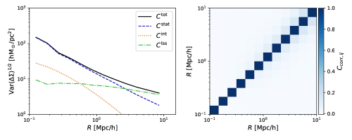
Figure 14: Left panel: diagonal components of the covariance matrix as a function of cluster-centric radius $R$ obtained from a stacked shear analysis based on Subaru Hyper Suprime-Cam observations. The black solid line shows the total covariance $C$; the blue dashed line is the uncertainty due to intrinsic shapes of source galaxies ($C^{\mathrm{stat}}$, denoted as $C^{\mathrm{shape}}$ in this paper), the orange dotted line is the covariance due to intrinsic variations of the projected cluster lensing signal ($C^{\mathrm{int}}$), and the green dashed-dotted line is the cosmic noise covariance due to large-scale structure uncorrelated with clusters ($C^{\mathrm{lss}}$). Shape noise is dominant for $R\lower 2.15277pt\hbox{$\;\buildrel<\over{\sim}\;$}3h^{-1}\mathrm{Mpc}$ (comoving), while the cosmic noise dominates at larger separations. Right panel: correlation matrix of the stacked total covariance as a function of the radial bin. The correlation between radial bins appears at large separation due to the cosmic noise covariance. Image reproduced with permission from Miyatake et al. (2019), copyright by AAS.

To obtain robust constraints on the underlying cluster mass distribution, we need to ensure that the shear likelihood function (Eq. (132)) includes all relevant sources of uncertainty (Gruen et al., 2015). Following Umetsu et al. (2016, 2020), we decompose the error covariance matrix $C$ for $\mbox{\boldmath$d$}=\{\langle g_{+}(\vartheta_{b})\rangle\}_{b=1}^{N_{\mathrm{bin}}}$ as:

$$C=C^{\mathrm{shape}}+C^{\mathrm{lss}}+C^{\mathrm{int}},$$ (133)

where $(C^{\mathrm{shape}})_{bb^{\prime}}=\sigma^{2}_{\mathrm{shape}}(\vartheta_{b})\delta_{bb^{\prime}}$ is the diagonal statistical uncertainty due to the shape noise (Eq. (120)); $(C^{\mathrm{lss}})_{bb^{\prime}}$ is the cosmic noise covariance due to uncorrelated large-scale structure projected along the line of sight (Schneider et al., 1998; Hoekstra, 2003); and $(C^{\mathrm{int}})_{bb^{\prime}}$ accounts for statistical fluctuations of the projected cluster lensing signal due to intrinsic variations associated with assembly bias and cluster asphericity (Gruen et al., 2015).

Figure 14 shows the diagonal elements of the covariance matrix used in a stacked weak-lensing analysis of Miyatake et al. (2019) and the correlation matrix, defined with the total covariance matrix as $C_{bb^{\prime}}/\sqrt{C_{bb}C_{b^{\prime}b^{\prime}}}$. A similar figure but for the $\kappa$ profile was presented in Umetsu et al. (2016), which presents a joint weak and strong lensing analysis of 20 high-mass clusters targeted by the CLASH survey (Cluster Lensing And Supernova survey with Hubble; Postman et al., 2012).

The elements of the $C^{\mathrm{lss}}$ matrix are given by (Hoekstra, 2003; Oguri and Takada, 2011):

$$(C^{\mathrm{lss}})_{bb^{\prime}}=\int\!\frac{\ell d\ell}{2\pi}P_{\kappa}(\ell)\hat{J_{2}}(\ell\vartheta_{b})\hat{J_{2}}(\ell\vartheta_{b^{\prime}}),$$ (134)

where $\hat{J}_{2}(\ell\vartheta_{b})$ is the Bessel function of the first kind and second order averaged over the $b$th annulus (for the case of the binned convergence profile, see Umetsu et al., 2011a, 2016; Gruen et al., 2015); and $P_{\kappa}(\ell)$ is the two-dimensional convergence power spectrum (see Eq. (37)) as a function of angular multipole $\ell$ calculated using the flat-sky and Limber’s approximation as (Limber, 1953; Kaiser, 1992):

$$P_{\kappa}(\ell)=\frac{9H_{0}^{4}\mathrm{\Omega}_{\mathrm{m}}^{2}}{4c^{4}}\int_{0}^{\chi_{s}}\!d\chi\,W^{2}(\chi,\chi_{s})a^{-2}(\chi)P_{\mathrm{NL}}\left[k=\frac{\ell}{r(\chi)};\chi\right],$$ (135)

with $\chi$ the comoving coordinate along the line of sight, $W(\chi,\chi_{s})=r(\chi_{s}-\chi)/r(\chi_{s})$ the ratio of angular diameter distances $D_{ls}/D_{s}$, and $P_{\mathrm{NL}}(k;\chi)$ the nonlinear matter power spectrum. The convergence power spectrum $P_{\kappa}(\ell)$ can be evaluated for a given source population and a cosmological model. In Eq. (135), we have assumed a single comoving distance $\chi_{s}$ corresponding to the effective single-plane redshift of source galaxies (i.e., all source galaxies lying at $\chi=\chi_{s}$). Provided that $\Delta\vartheta_{b}/\vartheta_{b}\ll 1$ with $\Delta\vartheta_{b}$ the radial bin width, we have $\hat{J}_{2}(\ell\vartheta_{b})\simeq J_{2}(\ell\vartheta_{b})$ (without bin-averaging) in Eq. (134).

The $C^{\mathrm{int}}$ matrix describes statistical fluctuations of the projected cluster lensing signal at fixed halo mass due to intrinsic variations in halo concentration, triaxiality and orientation, and correlated secondary structures around the cluster, as well as to deviations from the assumed NFW form (Becker and Kravtsov, 2011; Gruen et al., 2015). Gruen et al. (2015) constructed a semi-analytical model of $C^{\mathrm{int}}$ that is calibrated to cosmological numerical simulations. Umetsu et al. (2016) found that the diagonal part of the intrinsic covariance for the convergence $\kappa$ can be well approximated by:

$$(C^{\mathrm{int}}_{\kappa})_{bb}\simeq\alpha_{\mathrm{int}}^{2}\kappa^{2}(\vartheta_{b})$$ (136)

with $\alpha_{\mathrm{int}}=0.2$ in the intracluster (1-halo) regime at $R=D_{l}\vartheta\lower 2.15277pt\hbox{$\;\buildrel<\over{\sim}\;$}r_{\mathrm{200m}}$. This suggests that the intrinsic variance is self-similar in the sense that $\sqrt{(C^{\mathrm{int}}_{\kappa})_{bb}}/\kappa(\vartheta_{b})\sim\mathrm{const}$. A further simplification can be made by setting the off-diagonal elements of $C^{\mathrm{int}}_{\kappa}$ to zero, i.e., $(C^{\mathrm{int}}_{\kappa})_{bb^{\prime}}=\alpha^{2}_{\mathrm{int}}\kappa^{2}(\vartheta_{b})\delta_{bb^{\prime}}$. In general, the diagonal approximation to $C^{\mathrm{int}}_{\kappa}$ can lead to an underestimation of parameter uncertainties (Gruen et al., 2015, see their Fig. 5), where the degree of underestimation depends on the binning scheme, depth of weak-lensing observations, and halo mass. The impact of the diagonal approximation is more severe for deeper observations (or higher S/N weak-lensing data). Assuming a representative mass profile, it is possible to convert the intrinsic covariance matrix $C^{\mathrm{int}}_{\kappa}$ for the convergence into that for the tangential shear. This can be done by assuming an NFW density profile together with the concentration–mass relation $c_{\mathrm{200c}}(M_{\mathrm{200c}},z)$ for a given cosmological model (Miyatake et al., 2019; Umetsu et al., 2020). The covariance $C^{\mathrm{int}}$ for the $g_{+}$ profile obtained in this way thus depends on halo mass. Miyatake et al. (2019) found that, however, the intrinsic covariances with different halo masses remain nearly self-similar in their shapes once scaled by $R\to R/r_{\mathrm{200m}}$.

4.5 Stacked weak-lensing estimator

Stacking an ensemble of galaxy clusters helps average out large statistical fluctuations inherent in noisy weak-lensing observations of individual clusters. The statistical precision can be largely improved by stacking together a large number of clusters, allowing for tighter and more robust constraints on the ensemble properties of the cluster mass distribution. A stacked lensing analysis is thus complementary to an alternative approach that relies on individual cluster mass measurements (Sects. 4.2 and 4.4). In particular, a comparison of the two approaches provides a useful consistency check in different S/N regimes (e.g., Okabe et al., 2010; Umetsu et al., 2014, 2016, 2020; Okabe and Smith, 2016).

Let us consider an ensemble of $N$ galaxy clusters. We model the ensemble mass distribution of these clusters in terms of the excess surface mass density profile as:

$$\mbox{\boldmath$m$}=\left\{\Delta\Sigma(R_{b})\right\}_{b=1}^{N_{\mathrm{bin}}}.$$ (137)

Specifically, our model is a vector of $N_{\mathrm{bin}}$ parameters containing the binned $\Delta\Sigma(R)$ profile as a function of the projected cluster-centric radius $R$ (see Sect. 3.5). Here we aim to construct an unbiased estimator for the model $m$, or the ensemble $\Delta\Sigma(R)$ profile, given weak-lensing observations of $N$ individual clusters.

We assume that these clusters are distributed in redshift, having different geometric responses to the lensing signal through $\Sigma_{\mathrm{cr}}^{-1}(z_{l},z_{s})$. We express weak-lensing observations $\mbox{\boldmath$d$}_{l}=\{\langle g_{+}(R_{b}|z_{l})\rangle\}_{b=1}^{N_{\mathrm{bin}}}$ for a given cluster ($l$) as a sum of the signal vector $\mbox{\boldmath$s$}_{l}$ and the noise vector $\mbox{\boldmath$n$}_{l}$ as:

$$\mbox{\boldmath$d$}_{l}=\mbox{\boldmath$s$}_{l}+\mbox{\boldmath$n$}_{l}\ \ \ (l=1,2,\dots,N),$$ (138)

with

$$\mbox{\boldmath$s$}_{l}=a_{l}\mbox{\boldmath$m$},$$ (139)

where the response coefficient $a_{l}$ represents the source-averaged inverse critical surface mass density evaluated for the $l$th cluster (Eq. (99)):

$$a_{l}=\left\langle\Sigma_{\mathrm{cr},l}^{-1}\right\rangle.$$ (140)

In this expression, we assume that both $\mbox{\boldmath$d$}_{l}$ and $a_{l}$ have been averaged over an ensemble of source galaxies to represent the respective source-averaged quantities for the $l$th cluster. For simplicity, we have ignored the nonlinearity between the lensing signal $g_{+}$ and the surface mass density $\Delta\Sigma$ (see Sect. 3.6.2). We refer to Umetsu et al. (2020) for a treatment of the stacked weak-lensing analysis accounting for the nonlinear correction for the source-averaging effect.

Assuming that $n$ obeys Gaussian statistics and that the noise vectors between different clusters are statistically independent, we can write the total likelihood function of observations $\mbox{\boldmath$d$}=\{\mbox{\boldmath$d$}_{1},\mbox{\boldmath$d$}_{2},\dots,\mbox{\boldmath$d$}_{N}\}$ as:

$$P(\mbox{\boldmath$d$}|\mbox{\boldmath$m$})=\left(\prod_{l=1}^{N}{\cal N}_{l}\right)\exp{\left[-\frac{1}{2}\sum_{l=1}^{N}(\mbox{\boldmath$d$}_{l}-a_{l}\mbox{\boldmath$m$})^{t}C_{l}^{-1}(\mbox{\boldmath$d$}_{l}-a_{l}\mbox{\boldmath$m$})\right]},$$ (141)

where $C_{l}=\langle\mbox{\boldmath$n$}_{l}\mbox{\boldmath$n$}_{l}^{t}\rangle$ is the error covariance matrix (Sect. 4.4) for the $l$th cluster and ${\cal N}_{l}=(2\pi)^{-N_{\mathrm{bin}}/2}|C_{l}|^{-1/2}$ is a normalization factor. In ground-based cluster weak-lensing observations, the shear covariance matrix $(C_{l})_{bb^{\prime}}$ per cluster ($b,b^{\prime}=1,2,\dots,N_{\mathrm{bin}}$) is dominated by the statistical uncertainty due to the shape noise. The contribution from cosmic noise (Sect. 4.4) becomes important at large cluster-centric distances (Fig. 14).

The total log-likelihood function $\ln{P(\mbox{\boldmath$d$}|\mbox{\boldmath$m$})}$ is expressed as:

$$\ln{P(\mbox{\boldmath$d$}|\mbox{\boldmath$m$})}=-\frac{1}{2}\sum_{l=1}^{N}(\mbox{\boldmath$d$}_{l}-a_{l}\mbox{\boldmath$m$})^{t}C_{l}^{-1}(\mbox{\boldmath$d$}_{l}-a_{l}\mbox{\boldmath$m$})+\mathrm{const}.$$ (142)

According to Bayes’ theorem, the posterior probability distribution of $m$ given the data $d$ is:

$$P(\mbox{\boldmath$m$}|\mbox{\boldmath$d$})=P(\mbox{\boldmath$d$}|\mbox{\boldmath$m$})\frac{P(\mbox{\boldmath$m$})}{P(\mbox{\boldmath$d$})},$$ (143)

where $P(\mbox{\boldmath$m$})$ is the prior probability distribution for the model $m$ and $P(\mbox{\boldmath$d$})$ is the evidence that serves as a normalization factor here. We assume an uninformative uniform prior for our model $m$, such that $P(\mbox{\boldmath$m$}|\mbox{\boldmath$d$})\propto P(\mbox{\boldmath$d$}|\mbox{\boldmath$m$})$. By maximizing $\ln{P(\mbox{\boldmath$m$}|\mbox{\boldmath$d$})}$ with respect to $m$, we obtain the desired expression for the stacked weak-lensing estimator $\widehat{\mbox{\boldmath$m$}}$ as (e.g., Umetsu et al., 2011a):

$$\widehat{\mbox{\boldmath$m$}}=\left(\displaystyle\sum_{l=1}^{N}a_{l}^{2}C_{l}^{-1}\right)^{-1}\,\left(\displaystyle\sum_{l=1}^{N}{a_{l}C_{l}^{-1}\mbox{\boldmath$d$}_{l}}\right)\equiv\langle\!\langle\mbox{\boldmath$\Delta\Sigma$}_{+}\rangle\!\rangle.$$ (144)

Note that the weight assigned to $\Delta\Sigma_{+}$ of each cluster is proportional to $a_{l}^{2}=\left\langle\Sigma_{\mathrm{cr},l}^{-1}\right\rangle^{2}$ (see also Eq. (106)) because $\mbox{\boldmath$s$}_{l}\propto a_{l}$. The error covariance matrix ${\cal C}$ for the stacked estimator $\langle\!\langle\mbox{\boldmath$\Delta\Sigma$}_{+}\rangle\!\rangle$ (Eq. (144)) is given by:

$${\cal C}_{bb^{\prime}}=\left({F}^{-1}\right)_{bb^{\prime}},$$ (145)

with ${F}$ the Fisher information matrix defined as (e.g., Umetsu et al., 2011a):

$${F}_{bb^{\prime}}\equiv-{\cal E}\left[\frac{\partial^{2}\ln{P}(\mbox{\boldmath$m$}|\mbox{\boldmath$d$})}{\partial m_{b}\partial m_{b^{\prime}}}\right]_{\mbox{\boldmath$m$}=\widehat{\mbox{\boldmath$m$}}}=\left(\sum_{l=1}^{N}a_{l}^{2}C_{l}^{-1}\right)_{bb^{\prime}}.$$ (146)

The total S/N for detection is given by (e.g., Umetsu and Broadhurst, 2008):

$$(\mathrm{S/N})^{2}=\sum_{b,b^{\prime}=1}^{N_{\mathrm{bin}}}\widehat{m}_{b}\left({\cal C}^{-1}\right)_{bb^{\prime}}\widehat{m}_{b^{\prime}}=\widehat{\mbox{\boldmath$m$}}^{t}{\cal C}^{-1}\widehat{\mbox{\boldmath$m$}}.$$ (147)

Again, this quadratic S/N estimator breaks down and leads to an overestimation of significance if the actual per-bin S/N is less than unity (see Sect. 4.2).

It is noteworthy that interpreting the effective mass from the stacked lensing signal (Eq. (144)) requires caution especially when the cluster sample spans a wide range in mass and redshift. This is because the amplitude of the lensing signal is weighted by the redshift-dependent sensitivity and it is not linearly proportional to the cluster mass (e.g., Mandelbaum et al., 2005; Umetsu et al., 2016, 2020; Melchior et al., 2017; Sereno et al., 2017). We refer the reader to Miyatake et al. (2019) and Murata et al. (2019) for further discussion of this issue.

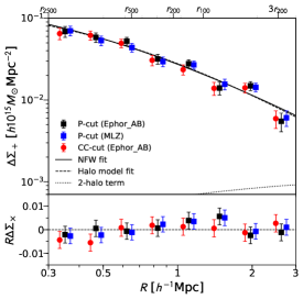
Figure 15: Stacked tangential ($\Delta\Sigma_{+}$: top) and cross ($\Delta\Sigma_{\times}$: bottom) shear profiles as a function of cluster-centric comoving radius $R$, derived for a sample of 136 spectroscopically confirmed X-ray-selected groups and clusters ($0.033\leqslant z_{l}\leqslant 1.033$) detected in the 25 deg² XXL-N region. The results are based on Subaru HSC-SSP survey data, shown for three different source-selection methods (black squares, blue squares, and red circles). The data points with different selection methods are horizontally shifted for visual clarity. The solid line and the dashed line represent the best-fit NFW model and the halo model, respectively, derived from the fiducial $P$-cut measurements. The dotted line shows the 2-halo term of the best-fit halo model. Ephor_AB and MLZ refer to HSC photo-$z$ codes (Tanaka et al., 2018). Image reproduced with permission from Umetsu et al. (2020), copyright by AAS.

Figure 15 shows the stacked weak-lensing signals around a sample of 136 spectroscopically confirmed X-ray groups and clusters at $0.033\leqslant z_{l}\leqslant 1.033$ selected from the XMM-XXL survey (Umetsu et al., 2020). Their weak-lensing analysis is based on HSC-SSP survey data. The figure compares stacked $\langle\!\langle\Delta\Sigma_{+}\rangle\!\rangle$ profiles of the XXL sample obtained with different source-selection methods (see Sect. 4.1). This comparison shows no significant difference between these profiles within errors in all bins. From a single-mass-bin NFW fit to the stacked shear profile, Umetsu et al. (2020) found $M_{\mathrm{200c}}=(8.7\pm 0.8)\times 10^{13}h^{-1}M_{\odot}$ and $c_{\mathrm{200c}}=3.5\pm 0.9$ at a lensing-weighted mean redshift of $z_{l}\approx 0.25$. This is in agreement with the mean concentration expected for dark matter halos in the standard $\mathrm{\Lambda}$CDM cosmology, $c_{\mathrm{200}}\approx 4.1$ at $M_{\mathrm{200c}}=8.7\times 10^{13}h^{-1}M_{\odot}$ and $z=0.25$ (e.g., Diemer and Joyce, 2019). Figure 15 also displays the best-fit halo model including the effects of surrounding large-scale structure as a 2-halo term. Figure 15 shows that the 2-halo term in the range $R\in[0.3,3]\,h^{-1}\mathrm{Mpc}$ (comoving) is negligibly small even in low-mass clusters and groups (e.g., Leauthaud et al., 2010; Covone et al., 2014; Sereno et al., 2015), for which the maximum radius corresponds to $\sim 3r_{\mathrm{200c}}$. This is because the tangential shear $\Delta\Sigma(R)=\overline{\Sigma}(R)-\Sigma(R)$ is insensitive to flattened sheet-like structures (Schneider and Seitz, 1995).

4.6 Quadrupole shear

Halos formed in collisionless CDM simulations are not spherical and can have complex shapes. A more realistic description of individual cluster halos is as triaxial ellipsoids with minor-to-major axis ratios of order $a/c\sim 0.5$, slowly increasing with halo-centric radius (Jing and Suto, 2002; Bonamigo et al., 2015). More massive halos are less spherical and more prolate, as they tend to form later. The projected matter distributions around clusters are thus expected to be anisotropic, with typical axis ratios of $q\sim 0.6$ (e.g., Okabe et al., 2018). The projected axis ratio of cluster halos varies slowly with cluster-centric distance (e.g., Okabe et al., 2018).

For sufficiently massive clusters at low redshift, deep weak-lensing observations allow us to constrain the halo shape on an individual cluster basis, by forward-modeling the observed two-dimensional shear (or convergence) field with elliptical lens models (Oguri et al., 2010; Okabe et al., 2011; Watanabe et al., 2011; Umetsu et al., 2012; Medezinski et al., 2013, 2016; Wegner et al., 2017). This tow-dimensional fitting approach is flexible and can be readily generalized to include multiple halo components (see the discussion in Sect. 3.6.1, e.g., Okabe et al., 2011; Medezinski et al., 2013) and triaxial halo shapes (e.g., Oguri et al., 2005; Sereno and Umetsu, 2011; Umetsu et al., 2015; Chiu et al., 2018).

In this subsection, we introduce quadrupole shear estimators for measuring the projected halo shape for a stacked ensemble of galaxy clusters.

4.6.1 Projected halo shape and multipole expansion

Following Adhikari et al. (2015), we introduce a formalism that allows for modeling the effects of halo ellipticity on weak shear observables based on an angular multipole expansion of the lensing fields. Let us write the azimuthally averaged projected mass density profile as $\Sigma^{(0)}(R)\propto R^{-\eta_{0}}$ with $\eta_{0}=-d\ln{\Sigma^{(0)}(R)/d\ln{R}}>0$. Assuming that $q$ is constant with cluster-centric radius, we can write the surface mass density around clusters as $\Sigma(x,y)\propto R_{q}^{-\eta_{0}}$ (Adhikari et al., 2015; Clampitt and Jain, 2016), where $R_{q}$ is an elliptical radial coordinate defined as (Evans and Bridle, 2009; Oguri et al., 2012; Umetsu et al., 2012, 2018):

$$R_{q}=\left(qx^{2}+y^{2}/q\right)^{1/2},$$ (148)

with $q$ the minor-to-major axis ratio $(0<q\leqslant 1)$. Here we have chosen the Cartesian coordinate system ($x,y$) centered on the halo, such that the $x$-axis is aligned with the major axis of the projected ellipse. We define the corresponding mass ellipticity by $e=(1-q^{2})/(1+q^{2})$.

We express the multipole expansion of $\Sigma$ as (Adhikari et al., 2015; Clampitt and Jain, 2016):

$$\Sigma(R,\varphi)\propto R_{q}^{-\eta_{0}} =R^{-\eta_{0}}\left[1+\frac{e\eta_{0}}{2}\cos{2\varphi}+O(e^{2})\right],$$ (149)

$$\equiv\Sigma^{(0)}(R)+\Sigma^{(2)}(R)\cos{2\varphi}+...,$$

where $\varphi$ is the azimuthal angle relative to the halo’s major axis, the multipole $\Sigma^{(m)}(R)$ is the coefficient of the $e^{im\varphi}$ component of the azimuthal behavior, and we assume $e\eta_{0}/2\ll 1$ to justify the neglect of higher-order terms in the expansion. We thus model the projected mass distributions of clusters as the sum of a monopole and a quadrupole. We further assume that:

$$e\simeq\frac{2\Sigma^{(2)}(R)}{\eta_{0}(R)\Sigma^{(0)}(R)}.$$ (150)

The quadrupole $\Sigma^{(2)}$ can thus be completely determined by the monopole $\Sigma^{(0)}\propto R^{-\eta_{0}}$, up to a multiplicative factor corresponding to the halo ellipticity $e$.

Similarly, the quadrupole moments of the tangential ($+$) and cross ($\times$) shear components are given by (Adhikari et al., 2015):

$$\Sigma_{\mathrm{cr}}\gamma_{+}^{(2)}(R) =\frac{e}{2}\left[-\Sigma^{(0)}(R)\eta_{0}(R)+I_{1}(R)+I_{2}(R)\right]\cos{2\varphi},$$ (151)

$$\Sigma_{\mathrm{cr}}\gamma_{\times}^{(2)}(R) =\frac{e}{2}\left[I_{1}(R)-I_{2}(R)\right]\sin{2\varphi},$$

where $I_{1}(R)$ and $I_{2}(R)$ are defined by (Clampitt and Jain, 2016):

$$I_{1}(R) =\frac{3}{R^{4}}\int_{0}^{R}\!R^{\prime 3}\Sigma^{(0)}(R^{\prime})\eta_{0}(R^{\prime})\,dR^{\prime},$$ (152)

$$I_{2}(R) =\int_{R}^{\infty}\!\frac{\Sigma_{0}(R^{\prime})\eta_{0}(R^{\prime})}{R^{\prime}}\,dR^{\prime}.$$

Equation (151) suggests an optimal estimator weighted by $\cos{2\varphi}$ to extract the quadrupole of the excess surface mass density, $\Delta\Sigma^{(2)}(R)$, from tangential shear measurements.

Weighted quadrupole estimators for the tangential and cross shear components are given by (Natarajan and Refregier, 2000; Mandelbaum et al., 2006):

$$\langle\!\langle\Delta\Sigma^{(2)}_{+}\rangle\!\rangle =\left[\sum_{l,s}w_{ls}\Delta\Sigma_{+}(R|z_{l},z_{s})\cos{2\varphi_{ls}}\right]\left[\sum_{l,s}w_{ls}\cos^{2}{2\varphi_{ls}}\right]^{-1},$$ (153)

$$\langle\!\langle\Delta\Sigma^{(2)}_{\times}\rangle\!\rangle =\left[\sum_{l,s}w_{ls}\Delta\Sigma_{\times}(R|z_{l},z_{s})\sin{2\varphi_{ls}}\right]\left[\sum_{l,s}w_{ls}\sin^{2}{2\varphi_{ls}}\right]^{-1},$$

where $\Delta\Sigma_{+,\times}(R|z_{l},z_{s})=\Sigma_{\mathrm{cr}}(z_{l},z_{s})g_{+,\times}(R|z_{l},z_{s})$ (Eq. (102)); $w_{ls}=\Sigma_{\mathrm{cr},ls}^{-2}/\sigma_{g,ls}^{2}$ is the statistical weight for each lens–source pair ($ls$), with $\sigma_{g,ls}$ the statistical uncertainty per shear component (see Eq. (106)); and $\varphi_{ls}$ is the azimuthal angle of each source galaxy ($s$) relative to the major axis of each cluster lens ($l$). In real observations, we must rely on the major axis of the distribution of baryonic tracers (e.g., central galaxies, X-ray gas) to perform aligned, stacked lensing measurements by Eq. (153) (Mandelbaum et al., 2006; van Uitert et al., 2012, 2017; Clampitt and Jain, 2016).

As discussed by Hoekstra et al. (2004) and Mandelbaum et al. (2006), in practical applications, Eq. (153) is susceptible to a possible systematic alignment of lens galaxy (e.g., BCGs) and source ellipticities. Such a spurious alignment signal can arise from an incomplete correction of the PSF anisotropy, which tends to affect neighboring objects in a similar manner. On the other hand, when interpreting the quadrupole shear signal, one must take into account possible misalignment between the underlying matter and tracer distributions, which will cause a dilution of the quadrupole shear signal. Moreover, modeling of the quadrupole shear based on the multipole expansion (Eq. (150)) should only be applied to the case with a small halo ellipticity ($e\eta/2\ll 1$), so that the higher-order terms can be safely ignored (see Eq. (149)).

4.6.2 Cartesian estimator

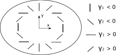
Figure 16: The quadrupole shear pattern produced by an elliptical mass distribution. The $x$-axis of the Cartesian coordinate system is aligned with the major axis of the tracer distribution, which is assumed to be aligned with the major axis of the underlying mass distribution. The sign convention for the Cartesian shear components ($\gamma_{1},\gamma_{2}$) is shown at the right. Note that the monopole shear (which is purely tangential) is not contributing to the shear pattern illustrated here. Image reproduced with permission from Clampitt and Jain (2016), copyright by the authors.

Now we introduce the Cartesian estimator of Clampitt and Jain (2016). Compared to the estimator of Natarajan and Refregier (2000), a practical advantage of this estimator is that one of the two Cartesian components ($\Delta\Sigma_{2}^{(\pm)}$ defined below) is insensitive to the spurious alignment of lens–source galaxy ellipticities (Clampitt and Jain, 2016) discussed at the end of Sect. 4.6.1. With this estimator, we measure the stacked quadrupole shear signal with respect to a coordinate system with the $x$-axis aligned with the major axis of the distribution of baryonic tracers (e.g., central galaxies, X-ray gas). The monopole signal is nulled with this Cartesian estimator. We adopt the same sign convention for the Cartesian $\gamma_{1}$ and $\gamma_{2}$ components as defined in Clampitt and Jain (2016) and use $\varphi$ to denote the azimuthal angle relative to the $x$-axis of each cluster. This is illustrated in Fig. 16.

The Cartesian shear components are related to the tangential and cross components (see Eq. (91)) by:

$$\gamma_{1}(R,\varphi) =-\gamma_{+}(R,\varphi)\cos{2\varphi}+\gamma_{\times}(R,\varphi)\sin{2\varphi},$$ (154)

$$\gamma_{2}(R,\varphi) =-\gamma_{+}(R,\varphi)\sin{2\varphi}-\gamma_{\times}(R,\varphi)\cos{2\varphi}.$$

In the framework of Adhikari et al. (2015) based on the multipole expansion, the multipole moments of the Cartesian shear components are written as follows (Clampitt and Jain, 2016):

$$\Sigma_{\mathrm{cr}}\gamma_{1}^{(2)} =\frac{e}{4}\left(\left[\Sigma^{(0)}(R)\eta_{0}(R)-2I_{1}(R)\right]\cos{4\varphi}+\Sigma^{(0)}(R)\eta_{0}(R)-2I_{2}(R)\right),$$ (155)

$$\Sigma_{\mathrm{cr}}\gamma_{2}^{(2)} =\frac{e}{4}\left[\Sigma^{(0)}(R)\eta_{0}(R)-2I_{1}(R)\right]\sin{4\varphi}.$$

Equation (155) shows that the azimuthal dependence of the Cartesian shear components goes as $\cos{4\varphi}$ (except for the two terms without $\varphi$ dependence; see Clampitt and Jain 2016 for more discussion) and $\sin{4\varphi}$, so that there is a sign change in both components after every angle $\pi/4$. When moving around the circle, the shear signal from elliptical clusters transitions between regions where $\gamma_{1}^{(2)}$ and then $\gamma_{2}^{(2)}$ alternately dominate (Clampitt and Jain, 2016), as illustrated in Fig. 16.

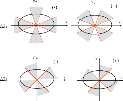
Figure 17: Illustration of the Cartesian quadrupole shear estimator of Clampitt and Jain (2016). The $x$-axis of the Cartesian coordinate system is aligned with the major axis of the tracer distribution (black solid ellipse). We group together the Cartesian first and second shear components in same-sign regions of $\cos{4\varphi}$ and $\sin{4\varphi}$ (gray-shaded regions), respectively, and define four quadrupole shear components, namely, $\Delta\Sigma_{1}^{(-)}$ (upper left), $\Delta\Sigma_{1}^{(+)}$ (upper right), $\Delta\Sigma_{2}^{(-)}$ (lower left), and $\Delta\Sigma_{2}^{(+)}$ (lower right). Image reproduced with permission from Umetsu et al. (2018), copyright by AAS.

Following Clampitt and Jain (2016), we group together the first and second shear components $(g_{1},g_{2})$ of background source galaxies in the regions where $\cos{4\varphi}$ and $\sin{4\varphi}$ have the same sign (see Fig. 17), respectively, and define the following estimator:

$$\langle\!\langle\Delta\Sigma_{i}^{(\pm)}(R)\rangle\!\rangle =\left[\sum_{l,s}w_{ls}\Delta\Sigma_{i}(R|z_{l},z_{s})\right]\left[\sum_{l,s}w_{ls}\right]^{-1}\ \ \ (i=1,2),$$ (156)

where we have introduced the notation in analogy to the tangential shear (Eq. (102)):

$$\Delta\Sigma_{i}(R|z_{l},z_{s})=\Sigma_{\mathrm{cr}}(z_{l},z_{s})g_{i}(R|z_{l},z_{s}),$$ (157)

where $w_{ls}=\Sigma_{\mathrm{cr},ls}^{-2}/\sigma_{g,ls}^{2}$ is the statistical weight for each lens–source pair ($ls$), with $\sigma_{g,ls}$ the statistical uncertainty per shear component (see Eq. (106)); and $s$ runs over all source galaxies that fall in the specified bin $(R,\varphi)$, different for each shear component $i$ and sign (Clampitt and Jain, 2016): $i=1$, $\mathrm{sign}=-$, $-\pi/8\leqslant\varphi<\pi/8$; $i=1$, $\mathrm{sign}=+$, $\pi/8\leqslant\varphi<3\pi/8$; $i=2$, $\mathrm{sign}=-$, $0\leqslant\varphi<\pi/4$; $i=2$, $\mathrm{sign}=+$, $\pi/4\leqslant\varphi<\pi/2$. For each case, the summation in Eq. (156) also includes source galaxies lying in symmetrical regions shifted by $\pi/2$, $\pi$, and $3\pi/2$, as illustrated in Fig. 17.

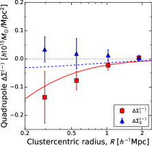
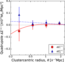
Figure 18: Stacked quadrupole shear profiles for a sample of 20 CLASH clusters measured with respect to the X-ray major axis of each cluster. Left panel: observed $\langle\!\langle\Delta\Sigma_{1}^{(-)}\rangle\!\rangle$ (red squares) and $\langle\!\langle\Delta\Sigma_{2}^{(-)}\rangle\!\rangle$ (blue triangles) profiles shown along with the best-fit elliptical-NFW model. Right panel: same as the left panel, but showing the results for the $\langle\!\langle\Delta\Sigma_{1,2}^{(+)}\rangle\!\rangle$ profiles. The best-fit model was obtained from a simultaneous elliptical-NFW fit to the four quadrupole shear profiles. Image reproduced with permission from Umetsu et al. (2018), copyright by AAS.

Figure 18 shows the stacked quadrupole shear profiles, $\langle\!\langle\Delta\Sigma_{1}^{(+)}\rangle\!\rangle$, $\langle\!\langle\Delta\Sigma_{1}^{(-)}\rangle\!\rangle$, $\langle\!\langle\Delta\Sigma_{2}^{(+)}\rangle\!\rangle$, and $\langle\!\langle\Delta\Sigma_{2}^{(-)}\rangle\!\rangle$, derived for a sample of 20 high-mass CLASH clusters (Umetsu et al., 2018). The quadrupole shear signal was measured with respect to the major axis of the X-ray gas shape of each cluster. Umetsu et al. (2018) modeled the stacked $\langle\!\langle\Delta\Sigma_{1,2}^{(\pm)}\rangle\!\rangle$ profiles by assuming an elliptical-NFW density profile with the major axis aligned with the X-ray major axis (for an elliptical extension of lensing mass models, see Keeton 2001). Any misalignment would thus lead to a dilution of the quadrupole signal and hence an underestimation of the halo ellipticity. Umetsu et al. (2018) obtained stacked constraints on the projected axis ratio of $q=0.67\pm 0.10$ (or $1-q=0.33\pm 0.10$), which is fully consistent with the median axis ratio $q=0.67\pm 0.07$ of this sample obtained from their two-dimensional shear and magnification analysis of the 20 individual clusters. Their results suggest that the total matter distribution is closely aligned with the X-ray brightness distribution (with a median misalignment angle of $|\Delta\mathrm{PA}|=21^{\circ}\pm 7^{\circ}$) as expected from cosmological hydrodynamical simulations (see Okabe et al., 2018).

5 Magnification bias

In addition to the shape distortions, gravitational lensing can cause focusing of light rays, which results in an amplification of the image flux through the solid-angle distortion (Sect. 2.6.3). Lensing magnification provides complementary and independent observational alternatives to gravitational shear, especially at high redshift where source galaxies are more difficult to resolve (Van Waerbeke et al., 2010; Hildebrandt et al., 2011; Ford et al., 2014; Chiu et al., 2016, 2020).

5.1 Magnified source counts

Let us consider source number counts $n_{0}(>F)$ per unit solid angle as a function of the limiting flux $F$ for a given population of background objects (e.g., color–magnitude-selected galaxies, quasars, etc.). In the absence of gravitational lensing, the intrinsic source counts can be written as:

$$n_{0}(>F)=\int\!dz\,\frac{d^{2}V}{dzd\Omega}\,\int_{L(z)}^{\infty}\!dL\,\frac{d^{2}N(L,z)}{dLdV}\equiv\int\!dz\,\frac{dn_{0}[z|>L(z)]}{dz},$$ (158)

where $d^{2}V(z)/dz/d\Omega$ is the comoving volume element per redshift interval per unit solid angle, $d^{2}N(L,z)/dL/dV$ is the luminosity function of the background population, $L(z)=4\pi D_{L}^{2}(z)F$ is the luminosity threshold corresponding to the flux limit $F$ at redshift $z$, with $D_{L}(z)$ the luminosity distance, and $dn_{0}[z|>L(z)]/dz$ is the redshift distribution function.

Here we focus on the subcritical regime with $\mu(\mbox{\boldmath$\theta$})>0$ (i.e., outside the critical curves). Lensing magnification causes focusing of light rays while conserving the surface brightness (Sect. 2.6.3), resulting in the following two competing effects (Broadhurst et al., 1995; Umetsu, 2013):

1. Area distortion: $\delta\Omega\to\mu(\mbox{\boldmath$\theta$})\delta\Omega$;

2. Flux amplification: $F\to\mu(\mbox{\boldmath$\theta$})F$.

The former effect reduces the geometric area in the source plane, thus decreasing the observed number of background sources per unit solid angle. On the other hand, the latter effect amplifies the flux of background sources, increasing the observed number of sources above the limiting flux.

In the presence of gravitational lensing, the magnified source counts are given as:

$$n_{\mu}(>F) =\int\!dz\,\frac{d^{2}V}{\mu(z)dzd\Omega}\,\int_{L(z)/\mu(z)}^{\infty}\!dL\,\frac{d^{2}N(L,z)}{dLdV}$$ (159)

$$=\int\!dz\,\frac{dn_{0}[z|>L(z)/\mu(z)]}{\mu(z)dz}\equiv\int\!dz\,\frac{dn_{\mu}[z|>L(z)]}{dz},$$

where $dn_{\mu}[z|>L(z)]/dz$ is the magnified redshift distribution function of the source population. Hence, the net change of the magnified source counts $n_{\mu}(>F)/n_{0}(>F)$, known as magnification bias, depends on the intrinsic (unlensed) source luminosity function, $d^{2}N(L,z)/dL/dV$. One can calculate the expectation value for the magnified source counts $n_{\mu}(>F)$ for a given background cosmology and a given source luminosity function.

In real observations, we apply different cuts (e.g., size, magnitude, and color cuts) in source selection for measuring the shear and magnification effects, thus leading to different source-redshift distributions. In contrast to the former effect, measuring the effect of magnification bias does not require source galaxies to be spatially resolved, but it does require a stringent flux limit against incompleteness effects (Hildebrandt, 2016; Chiu et al., 2020).

Equation (159) indicates that, when redshift information of individual source galaxies is available from spectroscopic redshifts, we can directly measure the magnified redshift distribution of background source galaxies for a flux-limited sample (Broadhurst et al., 1995):

$$\frac{dn_{\mu}[z|>L(z)]}{dz}=\frac{dn_{0}[z|>L(z)/\mu(z)]}{\mu(z)dz}.$$ (160)

Hence, in principle, the lensing-induced distortion of the redshift distribution $dn_{\mu}[z|>L(z)]/dz$ can be measured from spectroscopic-redshift measurements with respect to the unlensed distribution $dn_{0}[z|>L(z)]/dz$, which can be found in random fields. In particular, the integrated magnification-bias effect will translate into an enhancement in mean source redshift of the background sample (i.e., the first moment of Eq. (160)). Using 300,000 BOSS survey galaxies with accurate spectroscopic redshifts, Coupon et al. (2013) measured their mean redshift depth behind four large samples of optically selected clusters from the Sloan Digital Sky Survey (SDSS), totaling 5000–15,000 clusters. They found a $\lower 2.15277pt\hbox{$\;\buildrel>\over{\sim}\;$}1$ percent level of mean redshift increase $\delta z(R)$ toward the cluster center for SDSS-defined optical clusters with an effective mass of $M_{\mathrm{200c}}\sim(1-2)\times 10^{14}M_{\odot}$.

5.2 Magnification observables

To simplify the calculations, we discretize Eq. (159) as:

$$n_{\mu}(>F)\simeq\sum_{s}\frac{dn_{\mu}[z_{s}|>L(z_{s})]}{dz}\Delta z\equiv\sum_{s}n_{\mu}(z_{s}|>F),$$ (161)

where $n_{\mu}(z_{s}|>F)$ represents a subsample of the background population in the redshift interval $[z_{s},z_{s}+\Delta z]$. If the change in flux due to magnification is small compared to the range over which the slope of the luminosity function varies, the intrinsic source counts $n_{0}[z_{s}|>L(z_{s})]$ can be approximated at $L(z_{s})$ by a power law with a logarithmic slope of:

$$\alpha(z_{s})=-\frac{d\log n_{0}(z_{s}|>L)}{d\log L}\Big{|}_{L(z_{s})}.$$ (162)

The magnified source counts $n_{\mu}(z_{s}|>F)$ in the redshift interval $[z_{s},z_{s}+\Delta z]$ are given by:

$$n_{\mu}(z_{s}|>F) =\frac{1}{\mu}\frac{dn_{0}[z_{s}|>L(z_{s})/\mu]}{dz}\Delta z =n_{0}(z_{s}|>F)\,\mu^{\alpha(z_{s})-1}.$$ (163)

The corresponding magnification bias is given by:

$$b_{\mu}(z_{s}):=\frac{n_{\mu}(z_{s}|>F)}{n_{0}(z_{s}|>F)}=\mu^{\alpha-1}.$$ (164)

Equation (164) implies a positive bias for $\alpha>1$ and a negative bias for $\alpha<1$. The net magnification effect on the source counts vanishes at $\alpha=1$. For a depleted sample of background sources with $\alpha\ll 1$, the effect of magnification bias is dominated by the geometric area distortion ($b_{\mu}\to\mu^{-1}$ at $\alpha\to 0$) and insensitive to the intrinsic source luminosity function (Umetsu, 2013). In the weak-lensing limit ($|\gamma|,|\kappa|\ll 1$), we have:

$$b_{\mu}\simeq 1+2(\alpha-1)\kappa.$$ (165)

Hence, the flux magnification bias $b_{\mu}$ in the weak-lensing limit provides a local measure of the surface mass density field, $\kappa(\mbox{\boldmath$\theta$})$. The combination of shear and magnification can thus be used to break or alleviate mass-sheet degeneracy (Schneider et al., 2000; Broadhurst et al., 2005b; Umetsu and Broadhurst, 2008; Umetsu et al., 2011b, 2014, 2018).

In practical applications, we need to average over a broad range of source redshifts to increase the S/N. The magnification bias averaged over the source-redshift distribution is expressed as:

$$\langle b_{\mu}\rangle:=\frac{n_{\mu}(>F)}{n_{0}(>F)} =\frac{\sum_{s}n_{0}(z_{s}|>F)\mu^{\alpha(z_{s})-1}}{\sum_{s}n_{0}(z_{s}|>F)}.$$ (166)

In the continuous limit $\sum_{s}n_{0}(z_{s}|>F)\to\int\!dz\,dn_{0}(z|>F)/dz$, we have the following equation (Umetsu, 2013; Umetsu et al., 2016):

$$\langle b_{\mu}\rangle=\left[\int\!dz\,\frac{dn_{0}(z|>F)}{dz}\mu^{\alpha(z)-1}\right]\left[\int\!dz\,\frac{dn_{0}(z|>F)}{dz}\right]^{-1}=\langle\mu^{\alpha-1}\rangle.$$ (167)

Equation (167) gives a general expression for the flux magnification bias. Deep multi-band photometry spanning a wide wavelength range allows us to identify distinct populations of background galaxies (e.g., Medezinski et al., 2010, 2011, 2018b; Umetsu et al., 2012, 2014, 2015). Since a given flux limit ($F$) corresponds to different intrinsic luminosities $L(z_{s})$ at different source redshifts $z_{s}$ (Eq. (158)), source counts of distinctly different background populations probe different regimes of magnification bias. The bias is strongly negative for quiescent galaxies at $\langle z_{s}\rangle\sim 1$, with a faint-end slope of $\alpha\sim 0.4$ at the limiting magnitude $z^{\prime}\approx 25.6$ ABmag (e.g., Umetsu et al., 2014, 2015). A net count depletion ($b_{\mu}<1$) results for such a source population with $\alpha\ll 1$ (e.g., Broadhurst, 1995; Taylor et al., 1998; Broadhurst et al., 2005b; Umetsu and Broadhurst, 2008; Umetsu et al., 2011b, 2012, 2014, 2015; Ford et al., 2012; Coe et al., 2012; Medezinski et al., 2013; Radovich et al., 2015; Ziparo et al., 2016; Wong et al., 2017), because the effect of magnification bias is dominated by the geometric area distortion. In the regime of density depletion, a practical advantage is that the effect is not sensitive to the exact form of the source luminosity function. The S/N for detection of $b_{\mu}$ increases progressively as the flux limit $F$ decreases.

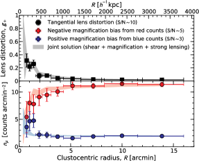
Figure 19: Weak-lensing radial profiles of MACS J1206.2$-$0847 ($z_{l}=0.439$) from Subaru Suprime-Cam observations. The top panel shows the reduced tangential shear profile $g_{+}$ (squares). The bottom panel shows the coverage- and masking-corrected number-count profiles $n_{\mu}$ for flux-limited samples of blue and red background galaxies (blue and red circles, respectively). The error bars include contributions from Poisson counting uncertainties and those from intrinsic angular clustering of each source population. For the red sample, a strong depletion of the source counts is seen toward the cluster center due to magnification of the sky area, while a slight enhancement of blue counts is present in the innermost radial bins due to the effect of positive magnification bias. Also shown for each observed profile is the joint Bayesian reconstruction (shaded area) from combined strong-lensing, weak shear lensing, and positive/negative magnification-bias measurements. Image reproduced with permission from Umetsu (2013), copyright by AAS.

Figure 19 displays weak-lensing radial profiles for the cluster MACS J1206.2$-$0847 at $z_{l}=0.439$ derived from Subaru Suprime-Cam observations (Umetsu, 2013). It is a highly massive X-ray cluster with $M_{\mathrm{200c}}=(11.1\pm 2.5)\times 10^{14}h^{-1}M_{\odot}$ (Umetsu et al., 2014) targeted by the CLASH survey. The black squares in the top panel show the reduced tangential shear profile $g_{+}(R)$. The blue and red circles in the bottom panel are positive and negative magnification-bias measurements $n_{\mu}(R)$ showing density enhancement and depletion, respectively, as a function of cluster-centric radius $R$. These weak-lensing measurements yield respective S/N values of $10.2$, $2.9$, and $4.7$. Figure 19 also shows a joint Bayesian reconstruction of each observed profile obtained from combined strong-lensing, weak shear lensing, and positive/negative magnification-bias measurements.

5.3 Nonlinear effects on the source-averaged magnification bias

It is instructive to consider a maximally depleted population of source galaxies with $\alpha=-d\log{n_{0}(>F)}/d\log{F}=0$ at the limiting flux $F$. For such a population, the effect of magnification bias is purely geometric, $\langle b_{\mu}\rangle=\langle\mu^{-1}\rangle$, and insensitive to details of the intrinsic source luminosity function, $d^{2}N(L,z)/dL/dz$. In the nonlinear subcritical regime, the source-averaged inverse magnification factor is expressed as (Umetsu, 2013):

$$\langle\mu^{-1}\rangle =\left\langle(1-\kappa)^{2}-|\gamma|^{2}\right\rangle$$ (168)

$$=\left(1-\langle\kappa\rangle\right)^{2}-|\langle\gamma\rangle|^{2}+(f_{l}-1)\left(\langle\kappa\rangle^{2}-|\langle\gamma\rangle|^{2}\right)$$

$$\equiv(1-\langle\kappa\rangle)^{2}-|\langle\gamma\rangle|^{2}+\Delta\langle\mu^{-1}\rangle,$$

where $\langle\cdots\rangle$ denotes the averaging over the source-redshift distribution (see Eq. (167)), $f_{l}=\langle\Sigma_{\mathrm{cr},l}^{-2}\rangle/\langle\Sigma_{\mathrm{cr},l}\rangle^{2}$ is a quantity of the order of unity, and $\Delta\langle\mu^{-1}\rangle$ is the correction with respect to the single source-plane approximation. The error associated with the single source-plane approximation is $\Delta\langle\mu^{-1}\rangle/\langle\mu^{-1}\rangle\simeq(f_{l}-1)\left(\langle\kappa\rangle^{2}-|\langle\gamma\rangle|^{2}\right)$, which is much smaller than unity for background populations with $\alpha\sim 0$ in the mildly nonlinear subcritical regime where $|\langle\kappa\rangle|\sim|\langle\gamma\rangle|\sim O(10^{-1})$. It is therefore reasonable to use the single source-plane approximation for calculating the magnification bias of depleted source populations with $\alpha\ll 0$.

In the regime of density enhancement ($\alpha>1$), on the other hand, interpreting the observed lensing signal requires detailed knowledge of the intrinsic source luminosity function (see, e.g., Chiu et al., 2016, 2020), especially in the nonlinear regime where the flux amplification factor is correspondingly large (say, $\mu\lower 2.15277pt\hbox{$\;\buildrel>\over{\sim}\;$}1.5$). For example, a blue distant population of background galaxies is observed to have a well-defined redshift distribution that is fairly symmetric and peaked at a mean redshift of $\langle z_{s}\rangle\sim 2$ (e.g., Lilly et al., 2007; Medezinski et al., 2010). Therefore, the majority of these faint blue galaxies are in the far background of typical cluster lenses, so that the lensing signal has a weaker dependence on the source redshift $z_{s}$. In such a case, the single source-plane approximation may well be justified (Umetsu, 2013).

5.4 Observational systematics and null tests

In real observations, contamination of the background sample by unlensed galaxies is a critical source of systematics in cluster weak lensing, as discussed in Sect. 4.1. In particular, contamination by cluster galaxies has a direct impact on the interpretation of background source counts because it will cause an apparent density enhancement at small cluster-centric radii. To avoid significant contamination and alleviate this problem as much as possible, one often relies on a stringent color–color selection (Sect. 4.1) to measure the lensing magnification signal from a distinct population of background galaxies (e.g., Broadhurst et al., 2005b; Umetsu and Broadhurst, 2008; Umetsu et al., 2011b, 2014; Ziparo et al., 2016; Chiu et al., 2016, 2020). If well-calibrated photo-$z$ PDFs are available from multi-band observations, the impact of cluster contamination can be characterized and assessed by statistically decomposing the photo-$z$ PDF $P(z)$ into the cluster and random-field populations (e.g., Gruen et al., 2014; Chiu et al., 2020).

Moreover, for unbiased magnification-bias measurements, one has to correct for the incomplete area coverage due to masked regions and incomplete measurement annuli. Specifically, masking (or blocking) of background galaxies by foreground objects, cluster members, and saturated or bad pixels needs to be properly accounted for (see Umetsu et al., 2011b; Chiu et al., 2020). Another concern is the impact of blending effects in the crowded regions of cluster environments and the presence of intracluster light (Gruen et al., 2019), which could bias the photometry and thus photo-$z$’s. The effects of masking and blending on the source counts can be examined and quantified by injecting synthetic galaxies into real images from observations (Huang et al., 2018; Chiu et al., 2020).

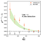
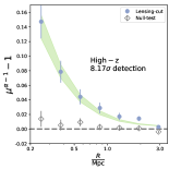
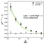
Figure 20: Stacked magnification-bias profiles around a sample of 3029 CAMIRA clusters obtained using low-$z$ (left) and high-$z$ (middle) samples, as well as the joint (right) background sample, from the Subaru HSC-SSP survey. The results are shown as a function of the projected physical cluster-centric radius $R$. Filled circles with error bars represent the stacked magnification-bias measurements with the respective lensing-cut samples. The total detection significance for each measurement is labeled in each panel. Open diamonds with error bars show the results for “null-test” samples, for which the net effect of magnification bias is expected to be zero. The green shaded region in each panel represents the $1\sigma$ confidence interval around the best-fit profile. Image reproduced with permission from Chiu et al. (2020), copyright by the authors.

Since the net effect of magnification bias is expected to vanish for a flux-limited background sample defined at $\alpha=1$ (Sect. 5.2), weak-lensing magnification provides a powerful null test, similar to the cross-shear ($B$-mode) signal in the case of weak shear lensing (Sect. 4.2). By performing a null test, one can empirically assess the level of residual bias that could be present in the measurement for a “lensing-cut” sample defined at $\alpha>1$ or $\alpha<1$. The only assumption made in this approach is that residual systematics are the same between the lensing-cut and null-test samples defined at different flux (magnitude) limits. This null test allows us to quantify the impact of deblending effects, biased photometry in crowded regions, and any incorrect assumptions about $P(z)$-decomposition (Chiu et al., 2020). This is demonstrated in Fig. 20. The figure shows the stacked magnification-bias profiles around a sample of 3029 CAMIRA clusters with richness $N>15$ in the redshift range $0.2\leqslant z<1.1$, obtained using flux-limited low-$z$ and high-$z$ background samples, as well as the joint sample, selected in the $g-i$ versus $r-z$ diagram from HSC-SSP survey data (Chiu et al., 2020). The magnification-bias signal for the full CAMIRA sample is detected at a significance level of $9.5\sigma$. On the other hand, the residual bias estimated from the null-test samples was found to be statistically consistent with zero (Chiu et al., 2020).

6 Recent advances in cluster weak-lensing observations

Galaxy clusters provide valuable information from the physics driving cosmic structure formation to the nature of dark matter and dark energy. Their content reflects that of the universe: $\sim 85\%$ dark matter and $\sim 15\%$ baryons (cf. $\mathrm{\Omega}_{\mathrm{b}}/\mathrm{\Omega}_{\mathrm{m}}=(15.7\pm 0.4)\%$; Planck Collaboration et al. 2016b), with $\sim 90\%$ of the baryons residing in a hot, X-ray-emitting phase of the intracluster medium. Massive clusters dominated by dark matter are not expected to be significantly affected by baryonic gas cooling (Blumenthal et al., 1986; Duffy et al., 2010), unlike individual galaxies, because the high temperature and low density prevent efficient cooling and gas contraction. Consequently, for clusters in a state of quasi-equilibrium, the form of their total mass profiles reflects closely the underlying dark matter distribution. Hence, galaxy clusters offer fundamental tests on the assumed properties of dark matter, as well as on models of nonlinear structure formation.

The $\mathrm{\Lambda}$CDM paradigm assumes that dark matter is effectively cold (nonrelativistic) and collisionless on astrophysical and cosmological scales (Bertone and Tait, 2018). In this context, the standard CDM model and its variants, such as self-interacting dark matter (SIDM; Spergel and Steinhardt, 2000) and wave dark matter ($\psi$DM; Peebles, 2000; Hu et al., 2000; Schive et al., 2014), can provide a range of testable predictions for the properties of cluster-size halos (Sects. 6.1 and 6.2). A prime example is the “Bullet Cluster”, a merging pair of clusters exhibiting a significant offset between the centers of the gravitational lensing mass and the X-ray peaks of the collisional cluster gas (Clowe et al., 2004, 2006). The data support that dark matter in clusters is effectively collisionless like galaxies, placing a robust upper limit on the self-interacting cross section for dark matter of $\sigma_{\mathrm{DM}}/m<1.25$ cm² g^-1 (Randall et al., 2008).

The abundance of clusters as a function of redshift provides a sensitive probe of the amplitude and growth rate of primordial density perturbations, as well as of the cosmological volume element $d^{2}V(z)/dz/d\Omega$. This cosmological sensitivity arises mainly because clusters populate the high-mass exponential tail of the halo mass function (e.g., Haiman et al., 2001). In principle galaxy clusters can complement other cosmological probes, such as CMB, galaxy clustering, cosmic shear, and distant supernova observations. To place cosmological constraints using clusters, however, it is essential to study large cluster samples with well-characterized selection functions, spanning a wide range in mass and redshift (Allen et al., 2004; Vikhlinin et al., 2009; Mantz et al., 2010). Currently, the ability of galaxy clusters to provide robust cosmological constraints is limited by systematic uncertainties in their mass calibration (Pratt et al., 2019). Since the level of mass bias is sensitive to calibration systematics of the instruments (Donahue et al., 2014; Israel et al., 2015) and is likely mass dependent (Sereno and Ettori, 2017; Umetsu et al., 2020), a concerted effort is needed to enable an accurate mass calibration with weak gravitational lensing (see Sect. 6.4).

Substantial progress has been made in constructing statistical samples of galaxy clusters thanks to dedicated wide-field surveys in various wavelengths (Planck Collaboration et al., 2014a, 2016a; Bleem et al., 2015; Miyazaki et al., 2018b; Oguri et al., 2018). Systematic lensing studies of galaxy clusters often target X-ray- or SZE-selected samples (e.g., von der Linden et al., 2014a; Postman et al., 2012; Gruen et al., 2014; Hoekstra et al., 2015; Sereno et al., 2017). This is because the hot intracluster gas provides an excellent tracer of the cluster’s gravitational potential (e.g., Donahue et al., 2014), except for the cases of massive cluster collisions caught in an ongoing phase of dissociative mergers (Clowe et al., 2006; Okabe and Umetsu, 2008). Moreover, X-ray and SZE observations provide useful centering information of individual clusters. The effect of off-centered clusters is to dilute and flatten the observed $\Sigma(R)$ profile at scales smaller than the offset scale $\sigma_{\mathrm{off}}$ (Johnston et al., 2007; George et al., 2012; Du and Fan, 2014). Since flattened, sheet-like mass distributions produce little shear, the impact of miscentering on $\Delta\Sigma(R)$ is much larger. The off-centered $\Delta\Sigma(R)$ profile is strongly suppressed by smoothing at scales $R\lower 2.15277pt\hbox{$\;\buildrel<\over{\sim}\;$}2.5\sigma_{\mathrm{off}}$ (Johnston et al., 2007). A comparison of X-ray, SZE, and optical (e.g., BCGs) center positions allows us to empirically assess the level of halo miscentering. It should be noted, however, that a merger can boost the X-ray and SZE signals and make their peaks off-centered during the compression phase (Molnar et al., 2012). Although the timescale on which this happens is expected to be short ($\sim 1$ Gyr; Ricker and Sarazin, 2001), it could induce a selection effect and contribute to the scatter in their scaling relations (Umetsu et al., 2020).

In this section, we review recent advances in our understanding of the distribution and amount of mass in galaxy clusters based on cluster weak-lensing observations.

6.1 Cluster mass distribution

The distribution and concentration of mass in dark-matter-dominated halos depend fundamentally on the properties of dark matter. For the case of collisionless CDM models, cosmological $N$-body simulations with sufficiently high resolution can provide accurate predictions for the end product of collisionless collapse in an expanding universe. Although the formation of halos is a complex, nonlinear dynamical process and halos are evolving through accretion and mergers, $\mathrm{\Lambda}$CDM models predict that the structure of quasi-equilibrium halos characterized in terms of the spherically averaged density profile $\rho(r)$ is approximately self-similar with a characteristic density cusp in their centers, $\rho(r)\propto 1/r$ (Navarro et al., 1996, 1997). The density profile $\rho(r)$ of dark-matter-dominated halos steepens continuously with radius and it is well described by the NFW form out to the virial radius, albeit with large variance associated with the assembly histories of individual halos (Jing and Suto, 2000).

Subsequent numerical studies with improved statistics and higher resolution found that the spherically averaged density profiles of $\mathrm{\Lambda}$CDM halos are better approximated by the three-parameter Einasto function with an additional degree of freedom (Merritt et al., 2006; Gao et al., 2008), which is closely linked with the mass accretion history of halos (Ludlow et al., 2013). The Einasto profile has a power-law logarithmic slope of $\gamma_{\mathrm{3D}}(r)=-2(r/r_{-2})^{\alpha_{\mathrm{E}}}$ (Sect. 4.3.3). For a given halo concentration, an Einasto profile with $\alpha_{\mathrm{E}}\approx 0.18$ closely resembles the NFW profile over roughly two decades in radius (Ludlow et al., 2013). The shape parameter $\alpha_{\mathrm{E}}$ of $\mathrm{\Lambda}$CDM halos increases gradually with halo mass and redshift (see Gao et al., 2008; Child et al., 2018, $0.15\lower 2.15277pt\hbox{$\;\buildrel<\over{\sim}\;$}\alpha_{\mathrm{E}}\lower 2.15277pt\hbox{$\;\buildrel<\over{\sim}\;$}0.25$ at $z=0$), so that the density profiles of $\mathrm{\Lambda}$CDM halos are not strictly self-similar (Navarro et al., 2010). By analyzing a large suite of $N$-body simulations in $\mathrm{\Lambda}$CDM, Child et al. (2018) found that both Einasto and NFW profiles provide a good description of the stacked mass distributions of cluster-size halos at low redshift, implying that the two fitting functions are nearly indistinguishable for stacked ensembles of low-redshift clusters, in contrast to clusters at higher redshift ($z\lower 2.15277pt\hbox{$\;\buildrel>\over{\sim}\;$}1$).

The three-dimensional shape of collisionless halos is predicted to be generally triaxial with a preference for prolate shapes (Warren et al., 1992; Jing and Suto, 2002), reflecting the collisionless nature of dark matter (Ostriker and Steinhardt, 2003). Older halos tend to be more relaxed and thus to be rounder. Since more massive halos form later on average, cluster-size halos are expected to be more elongated than less massive systems (Shaw et al., 2006; Ho et al., 2006; Despali et al., 2014, 2017; Bonamigo et al., 2015). Accretion of matter from the surrounding large-scale environment also plays a key role in determining the shape and orientation of halos. The halo orientation tends to be in the preferential infall direction of the subhalos and hence aligned along the surrounding filaments (Shaw et al., 2006). The shape and orientation of galaxy clusters thus provide an independent test of models of structure formation (see Sect. 4.6).

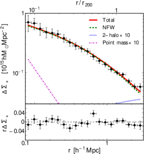
Figure 21: Stacked tangential ($\Delta\Sigma_{+}$: top) and cross ($\Delta\Sigma_{\times}$: bottom) shear profiles obtained for a sample of 50 X-ray luminous LoCuSS clusters. Solid red and dashed green lines are the total mass model and the NFW model, respectively. The dotted blue and dash-dotted magenta lines represent the 2-halo term and the central point source multiplied by a factor of 10, respectively. Image reproduced with permission from Okabe and Smith (2016), copyright by the authors.

Prior to dedicated wide-field optical imaging surveys such as Subaru HSC-SSP and DES, several cluster lensing surveys carried out deep targeted observations toward a few tens to several tens of highly massive galaxy clusters with $M_{\mathrm{200c}}\sim 10^{15}M_{\odot}$ (e.g., Postman et al., 2012; Okabe et al., 2013; von der Linden et al., 2014a; Hoekstra et al., 2015). Since such clusters are extremely rare across the sky, targeted weak-lensing observations with deep multi-band imaging currently represent the most efficient approach to study in detail the high-mass population of galaxy clusters each with sufficiently high S/N (see Contigiani et al., 2019).

In the last decade, cluster–galaxy weak-lensing observations have established that the total matter distribution within clusters in projection can be well described by cuspy, outward-steepening density profiles (Umetsu et al., 2011b, 2014, 2016; Beraldo e Silva et al., 2013; Newman et al., 2013b; Okabe et al., 2013; Sereno et al., 2017), such as the NFW and Einasto profiles with a near-universal shape (Niikura et al., 2015; Umetsu and Diemer, 2017), as predicted for collisionless halos in quasi-gravitational equilibrium (e.g., Navarro et al., 1996, 1997; Taylor and Navarro, 2001; Merritt et al., 2006; Gao et al., 2008; Hjorth and Williams, 2010; Williams and Hjorth, 2010). Moreover, the shape and orientation of galaxy clusters as constrained by weak-lensing and multiwavelength data sets are found to be in agreement with $\mathrm{\Lambda}$CDM predictions (e.g., Oguri et al., 2005; Evans and Bridle, 2009; Oguri et al., 2010; Morandi et al., 2012; Sereno et al., 2013, 2018b; Umetsu et al., 2015, 2018; Chiu et al., 2018; Shin et al., 2018), although detailed studies of individual clusters are currently limited to a relatively small number of high-mass clusters with deep multiwavelength observations (see Sereno et al., 2018b; Umetsu et al., 2018). These results are all in support of the standard explanation for dark matter as effectively collisionless and nonrelativistic on sub-megaparsec scales and beyond, with an excellent match with standard $\mathrm{\Lambda}$CDM predictions (however, see Meneghetti et al., 2020, for an excess of galaxy–galaxy strong-lensing events in clusters with respect to $\mathrm{\Lambda}$CDM).

In Fig. 21, we show the ensemble-averaged $\langle\!\langle\Delta\Sigma_{+}\rangle\!\rangle$ profile in the radial range $R\in[0.1,2.8]\,h^{-1}\mathrm{Mpc}$ obtained for a stacked sample of 50 X-ray clusters (Okabe and Smith, 2016) targeted by the LoCuSS Survey (Local Cluster Substructure Survey; Smith et al., 2016). Their weak shear lensing analysis is based on two-band imaging observations with Subaru/Suprime-Cam. Their cluster sample is drawn from the ROSAT All-Sky Survey (RASS; Voges et al., 1999) at $0.15<z<0.3$ and is approximately X-ray luminosity limited. The stacked shear profile of the LoCuSS sample is in excellent agreement with the NFW profile with $M_{\mathrm{200c}}=6.37^{+0.28}_{-0.27}\times 10^{14}h^{-1}M_{\odot}$ and $c_{\mathrm{200c}}=3.69^{+0.26}_{-0.24}$ at $z_{l}=0.23$. The 2-halo term contribution to $\Delta\Sigma$ for the LoCuSS sample is negligibly small in the radial range $\lower 2.15277pt\hbox{$\;\buildrel<\over{\sim}\;$}2r_{\mathrm{200c}}$. From a single Einasto profile fit to the stacked $\langle\!\langle\Delta\Sigma\rangle\!\rangle$ profile, Okabe and Smith (2016) obtained the best-fit Einasto shape parameter of $\alpha_{\mathrm{E}}=0.161^{+0.042}_{-0.041}$, which is consistent within the errors with the $\mathrm{\Lambda}$CDM predictions for cluster-size halos at $z_{l}=0.23$ (Gao et al., 2008; Dutton and Macciò, 2014).

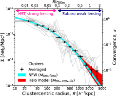
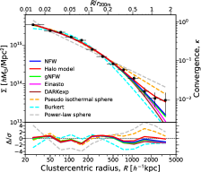
Figure 22: Left panel: ensemble-averaged projected mass density profile $\langle\!\langle\Sigma(R)\rangle\!\rangle$ (black squares) for a sample of 16 CLASH X-ray-selected clusters (gray lines), obtained from a joint analysis of strong-lensing, weak-lensing shear and magnification data. Right panel: models with $\chi^{2}$ probabilities to exceed (PTE) of $>0.05$ are shown with solid lines, while those with $\mathrm{PTE}\leqslant 0.05$ are shown with dashed lines. The averaged mass profile is well described by a family of density profiles predicted for dark-matter-dominated halos in gravitational equilibrium, such as the NFW, Einasto, and DARKexp models. Cuspy halo models (red) that include the 2-halo contribution from surrounding large-scale structure provide improved agreement with the data. This is a slightly modified version of the figure presented in Umetsu et al. (2016).

Figure 22 shows the ensemble-averaged $\langle\!\langle\Sigma\rangle\!\rangle$ profile of 16 CLASH X-ray-selected clusters (Umetsu et al., 2016) based on a joint strong and weak lensing analysis of 16-band Hubble Space Telescope (HST) observations (Zitrin et al., 2015) and wide-field multicolor imaging taken primarily with Subaru/Suprime-Cam (Umetsu et al., 2014). The CLASH survey is an HST Multi-Cycle Treasury program designed to study with 525 assigned orbits the mass distributions of 25 high-mass clusters. In this sample, 20 clusters were selected to have regular X-ray morphologies and X-ray temperatures above 5 keV. Numerical simulations suggest that this X-ray-selected subsample is mostly composed of relaxed clusters ($\sim 70\%$) but the rest ($\sim 30\%$) are unrelaxed systems (Meneghetti et al., 2014). Another subset of five clusters were selected by their high-magnification lensing properties. Umetsu et al. (2016) studied a subset of 20 CLASH clusters (16 X-ray-selected and 4 high-magnification systems) taken from Umetsu et al. (2014), who presented a joint shear and magnification weak-lensing analysis of these individual clusters. The stacked $\langle\!\langle\Sigma\rangle\!\rangle$ profile over two decades in radius, $R\in[0.02,2]r_{\mathrm{200m}}$, is well described by a family of density profiles predicted for cuspy dark-matter-dominated halos in gravitational equilibrium, namely, the NFW, Einasto, and DARKexp models (Umetsu et al., 2016). In contrast, the single power-law, cored-isothermal, and Burkert density profiles are statistically disfavored by the data. Cuspy halo models that include the 2-halo term provide improved agreement with the data.

Umetsu et al. (2016) found the best-fit NFW parameters for the stacked CLASH $\langle\!\langle\Sigma\rangle\!\rangle$ profile of $M_{\mathrm{200c}}=10.1^{+0.8}_{-0.7}\times 10^{14}h^{-1}M_{\odot}$ and $c_{\mathrm{200c}}=3.76^{+0.29}_{-0.27}$ (Umetsu et al., 2016) at a lensing-weighted mean redshift of $z_{l}\approx 0.34$. Similarly, the best-fit Einasto shape parameter for the stacked $\langle\!\langle\Sigma\rangle\!\rangle$ profile is $\alpha_{\mathrm{E}}=0.232^{+0.042}_{-0.038}$, which is in excellent agreement with predictions from $\mathrm{\Lambda}$CDM numerical simulations, $\alpha_{\mathrm{E}}=0.21\pm 0.07$ (Meneghetti et al., 2014, $\alpha_{\mathrm{E}}=0.24\pm 0.09$ when fitted to surface mass density profiles of projected halos).

Note that the innermost bin in Fig. 22 represents the mean density interior to $R_{\mathrm{min}}=40h^{-1}\mathrm{kpc}$ corresponding to the typical resolution limit of their HST strong-lensing analysis, $\delta\vartheta\approx 10$ arcsec. This scale $R_{\mathrm{min}}$ is about twice the typical half-light radius of the CLASH BCGs (see Tian et al., 2020), within which the stellar baryons dominate the total mass of the clusters (e.g., Caminha et al., 2019). Determinations of the central slope of the dark matter density profile $\rho_{\mathrm{DM}}(r)$ in clusters require additional constraints on the total mass in the innermost region, such as from stellar kinematics of the BCG (Newman et al., 2013a). To constrain $\rho_{\mathrm{DM}}(r)$, one needs to carefully model the different contributions to the cluster total mass profile, coming from the stellar mass of member galaxies, the hot gas component, the BCG stellar mass, and dark matter (Sartoris et al., 2020). Moreover, it is important to take into account the velocity anisotropy on the interpretation of the line-of-sight stellar velocity dispersion profile of the BCG (Schaller et al., 2015; Sartoris et al., 2020; He et al., 2020). For these reasons, current measurements and interpretations of the asymptotic central slope of $\rho_{\mathrm{DM}}(r)$ in galaxy clusters appear to be controversial (e.g., Newman et al., 2013a; Sartoris et al., 2020; He et al., 2020).

According to cosmological $N$-body simulations, the spherically averaged density profiles in the halo outskirts are most self-similar when expressed in units of overdensity radii $r_{\Delta_{\mathrm{m}}}$ defined with respect to the mean density of the universe, $\overline{\rho}(z)$, especially to $r_{\mathrm{200m}}$ (Diemer and Kravtsov, 2014). This self-similarity indicates that overdensity radii defined with respect to the mean cosmic density are preferred to describe the structure and evolution of the outer density profiles. The structure and dynamics of the infall region are expected to be universal in units of the turnaround radius, according to self-similar infall models (Gunn and Gott, 1972; Fillmore and Goldreich, 1984; Bertschinger, 1985; Shi, 2016). In these models, the turnaround radius is a fixed multiple of the radius enclosing a given fixed overdensity with respect to the mean cosmic density. The outer profiles can thus be expected to be self-similar in $r/r_{\mathrm{200m}}$. In contrast, the density profiles in the intra-halo (1-halo) region are found to be most self-similar when they are scaled by $r_{\mathrm{200c}}$ (or any other critical overdensity radius with a reasonable threshold; Diemer and Kravtsov, 2014). That is, density profiles of $\mathrm{\Lambda}$CDM halos in $N$-body simulations prefer different scaling radii in different regions of the density profile (Diemer and Kravtsov, 2014). These empirical scalings were confirmed in cosmological hydrodynamical simulations of galaxy clusters (Lau et al., 2015, see also Shi 2016). However, the physical explanation for the self-similarity of the inner density profile when rescaled with $r_{\mathrm{200c}}$ is less clear.

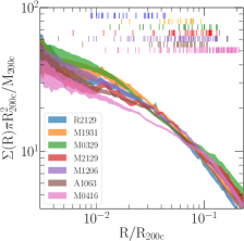
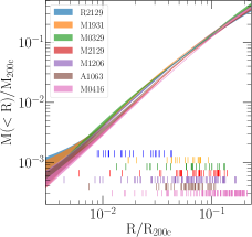
Figure 23: Projected mass density (left) and enclosed mass (right) profiles for seven CLASH clusters derived from a detailed strong-lensing analysis, rescaled by $M_{\mathrm{200c}}$ and $r_{\mathrm{200c}}$ obtained from NFW fits to independent weak-lensing measurements (Umetsu et al., 2018). Vertical lines color-coded for each cluster indicate the positions of multiple images used for the lens modeling, all belonging to spectroscopic confirmed families. MACS J0416 with a shallower inner density slope is a highly asymmetric merging system. Image reproduced with permission from Caminha et al. (2019), copyright by ESO.

In Fig. 23, we show the projected total mass density ($\Sigma$) and enclosed mass ($M_{\mathrm{2D}}$) profiles for seven CLASH clusters derived from a detailed strong-lensing analysis of Caminha et al. (2019) based on extensive spectroscopic information, primarily from the Multi Unit Spectroscopic Explorer (MUSE) archival data complemented with CLASH-VLT redshift measurements (Biviano et al., 2013; Rosati et al., 2014). In the figure, the projected mass profiles of individual clusters are rescaled using $M_{\mathrm{200c}}$ and $r_{\mathrm{200c}}$ obtained from NFW fits to independent ground-based weak-lensing measurements (Umetsu et al., 2018). All clusters have a relatively large number of multiple-image constraints in the region $10^{-2}\lower 2.15277pt\hbox{$\;\buildrel<\over{\sim}\;$}R/r_{\mathrm{200c}}\lower 2.15277pt\hbox{$\;\buildrel<\over{\sim}\;$}10^{-1}$, where the shapes of the rescaled $\Sigma(R)$ and $M_{\mathrm{2D}}(<R)$ profiles are remarkably similar. Even MACS J0416 (Zitrin et al., 2013; Jauzac et al., 2015; Grillo et al., 2015; Balestra et al., 2016), which is a highly asymmetric merging system, does not deviate significantly from the overall homologous profiles. Within $10\%$ and $20\%$ of $r_{\mathrm{200c}}$ for the seven clusters, Caminha et al. (2019) measured a mean projected total mass value of $0.13$ and $0.32\times M_{\mathrm{200c}}$, respectively, finding a remarkably small scatter of $5\%$ and $6\%$. At these same radii, for the projected total mass density profiles, they found a mean value of $9.0$ and $4.7\times M_{\mathrm{200c}}/(\pi r_{\mathrm{200c}}^{2})$, with a slightly larger scatter of $7\%$ and $9\%$, respectively. The observed trend is qualitatively consistent with the predictions by Diemer and Kravtsov (2014) and Lau et al. (2015).

6.2 The concentration–mass relation

The halo concentration $c_{\Delta}$ is a key quantity that characterizes the density structure of dark matter halos, where $c_{\Delta}$ is defined as the ratio of the outer halo radius $r_{\Delta}$ (typically defined at an overdensity of $\Delta_{\mathrm{c}}=200$) and the inner characteristic radius $r_{\mathrm{s}}$ at which the logarithmic density slope is $-2$ (Sect. 4.2). The halo concentration as a function of halo mass and redshift is referred to as the concentration–mass ($c$–$M$) relation (e.g., Bullock et al., 2001; Wechsler et al., 2002). For NFW halos, the $c$–$M$ relation fully specifies the structure of halos at fixed halo mass and thus is a key ingredient of cluster cosmology.

In hierarchical $\mathrm{\Lambda}$CDM models, $c_{\Delta}$ is predicted to depend on the accretion history. In the early phase of rapid mass accretion, the scale radius $r_{\mathrm{s}}$ of a halo scales approximately as the virial radius and thus $c_{\Delta}$ remains nearly constant (Zhao et al., 2003). During the subsequent slow accretion phase, the scale radius stays approximately constant, whereas $r_{\Delta}$ continues to grow through a mixture of physical accretion and pseudo-evolution, resulting in an increase in halo concentration (Navarro et al., 1997; Bullock et al., 2001; Wechsler et al., 2002; Diemer et al., 2013; Correa et al., 2015). Since the mass accretion history depends on the amplitude and shape of peaks in the initial density field, as well as on the mass scale and the background cosmology, $c_{\Delta}$ depends on halo mass, redshift, and cosmological parameters (Prada et al., 2012; Dutton and Macciò, 2014; Diemer and Kravtsov, 2015; Diemer and Joyce, 2019). There have been a number of attempts to obtain a more universal representation of $c_{\Delta}$ as a function of physical parameters, such as the halo peak height $\nu(M_{\Delta},z)$ and the local slope of the matter power spectrum $d\ln{P(k)}/d\ln{k}$ (see Zhao et al., 2009; Prada et al., 2012; Diemer and Kravtsov, 2015; Diemer and Joyce, 2019).

Since galaxy clusters are, on average, dynamically young and still growing through accretion and mergers, cluster halos are expected to have relatively low concentrations, $c_{\mathrm{200c}}(z=0)\sim 4$, in contrast to individual galaxy halos that have denser central regions, $c_{\mathrm{200c}}(z=0)\sim 7-8$ (Bhattacharya et al., 2013; Dutton and Macciò, 2014; Diemer and Kravtsov, 2015; Child et al., 2018; Diemer and Joyce, 2019). These general trends are complicated by diverse formation and assembly histories of individual halos (Ludlow et al., 2013), which translate into substantial scatter in the $c$–$M$ relation, with a lognormal intrinsic dispersion of $\sigma_{\mathrm{int}}(\ln{c_{\mathrm{200c}}})\sim 35\%$ at fixed halo mass (e.g., Duffy et al., 2008; Bhattacharya et al., 2013; Diemer and Kravtsov, 2015)

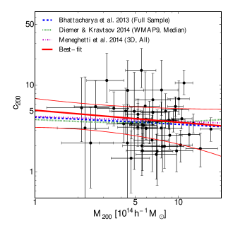
Figure 24: The concentration–mass ($c_{\mathrm{200c}}$–$M_{\mathrm{200c}}$) relation for a sample of 50 X-ray luminous clusters (black circles with error bars) derived from the LoCuSS survey (Okabe and Smith, 2016). The results are based on weak-lensing measurements from Subaru Suprime-Cam observations. The thick and thin red lines show the best-fitting function and the errors, respectively. The dashed blue, dotted green, and dot-dashed magenta lines are the mean $c$–$M$ relation of $\mathrm{\Lambda}$CDM halos derived from numerical simulations of Bhattacharya et al. (2013), Diemer and Kravtsov (2015), and Meneghetti et al. (2014) at $z_{l}=0.23$, respectively. Image reproduced with permission from Okabe and Smith (2016), copyright by the authors.

On the observational side, cluster lensing studies targeting lensing-unbiased samples (e.g., Merten et al., 2015; Du et al., 2015; Umetsu et al., 2016, 2020; Okabe and Smith, 2016; Cibirka et al., 2017; Sereno et al., 2017; Klein et al., 2019) have found that the $c$–$M$ relations derived for these cluster samples agree well with theoretical models calibrated for recent $\mathrm{\Lambda}$CDM cosmologies (e.g., Bhattacharya et al., 2013; Dutton and Macciò, 2014; Meneghetti et al., 2014; Diemer and Kravtsov, 2015; Child et al., 2018; Diemer and Joyce, 2019).

In Fig. 24, we show the $c_{\mathrm{200c}}$–$M_{\mathrm{200c}}$ relation derived from a Subaru weak-lensing analysis of 50 X-ray-selected clusters targeted by the LoCuSS survey (see Sect. 6.1; Okabe and Smith, 2016). Their results are based on NFW profile fits to the reduced tangential shear profiles of individual clusters. The best-fit $c_{\mathrm{200c}}$–$M_{\mathrm{200c}}$ relation for the LoCuSS sample is $c_{\mathrm{200c}}=5.12^{+2.08}_{-1.44}\times(M_{\mathrm{200c}}/10^{14}h^{-1}M_{\odot})^{-0.14\pm 0.16}$ at $z_{l}=0.23$ (Okabe and Smith, 2016). The normalization and slope of the $c_{\mathrm{200c}}$–$M_{\mathrm{200c}}$ relation for the LoCuSS sample are in excellent agreement with those found for mass-selected samples of dark-matter halos in $\mathrm{\Lambda}$CDM numerical simulations (Bhattacharya et al., 2013; Meneghetti et al., 2014; Diemer and Kravtsov, 2015), indicating no significant impact of the X-ray selection on the normalization and mass slope parameters. Okabe and Smith (2016) found an intrinsic lognormal dispersion of $\sigma_{\mathrm{int}}(\ln{c_{\mathrm{200c}}})<20\%$ ($68.3\%$ CL) at fixed halo mass, which is lower than found for $\mathrm{\Lambda}$CDM halos in $N$-body simulations ($\sim 35\%$ for the full population of halos including both relaxed and unrelaxed systems; Bhattacharya et al., 2013; Diemer and Kravtsov, 2015). Similar results on the concentration scatter were obtained for independent X-ray cluster samples (e.g., the CLASH and the XXL samples with $\sigma_{\mathrm{int}}(\ln{c_{\mathrm{200c}}})=(13\pm 6)\%$ and $\sigma_{\mathrm{int}}(\ln{c_{\mathrm{200c}}})<24\%$ at the $99.7\%$ CL, respectively; see Umetsu et al., 2016, 2020). This is likely caused in part by the X-ray selection bias in terms of the cool-core or relaxation state, as found by previous studies (Buote et al., 2007; Ettori et al., 2010; Eckert et al., 2011; Meneghetti et al., 2014).

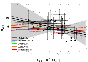
Figure 25: The concentration–mass ($c_{\mathrm{200c}}$–$M_{\mathrm{200c}}$) relation at $z_{l}=0.20$, derived from a weak-lensing analysis of 35 PSZ2LenS clusters (Sereno et al., 2017) selected from the Planck SZE survey. The solid and dashed black lines show the median $c$–$M$ relation and its intrinsic scatter, respectively. The shaded gray region encloses the $68.3\%$ probability around the median relation due to uncertainties on the scaling parameters. The blue, green, and orange lines show the $c$–$M$ relation of $\mathrm{\Lambda}$CDM halos derived from numerical simulations of Bhattacharya et al. (2013), Dutton and Macciò (2014), and Ludlow et al. (2016), respectively. The solid and dashed red lines show the $c$–$M$ relation of $\mathrm{\Lambda}$CDM halos and its $1\sigma$ scatter, respectively, from Meneghetti et al. (2014). Image reproduced with permission from Sereno et al. (2017), copyright by the authors.

Cluster samples are traditionally defined by X-ray or optical observables, and more recently through the thermal SZE strength (e.g., Planck Collaboration et al., 2016a). The SZE is a characteristic spectral distortion in the CMB induced by inverse Compton scattering between cold CMB photons and hot ionized electrons (Sect. 2.6.5; Rephaeli, 1995; Birkinshaw, 1999). Unlike any other detection techniques, SZE-selected cluster samples are nearly mass-limited and have well-behaved selection functions. This is because the SZE detection signal has a very weak dependence on the redshift (see Eq. (38)) and it is also less sensitive to the relaxation state of the cluster. Blind SZE surveys can thus provide representative cluster samples representative of the full population of halos out to high redshift. This makes SZE surveys ideal for cosmological tests based on the evolution of the cluster abundance.

We show in Fig. 25 the $c_{\mathrm{200c}}$–$M_{\mathrm{200c}}$ relation at $z_{l}=0.20$ obtained for a sample of Planck clusters targeted by the PSZ2LenS project (Sereno et al., 2017). The PSZ2LenS sample includes 35 optically confirmed Planck clusters selected from the second Planck catalog of Sunyaev–Zel’dovich sources (PSZ2; Planck Collaboration et al., 2016a) located in the fields of two lensing surveys, namely the CFHTLenS (Canada France Hawaii Telescope Lensing Survey; Heymans et al., 2012) and RCSLenS (Red Cluster Sequence Lensing Survey; Hildebrandt et al., 2016) surveys. The PSZ2LenS sample represents a faithful subsample of the whole population of Planck clusters, for which homogeneous weak-lensing data and photometric redshifts are available from the CFHTLenS and RCSLenS surveys (Sereno et al., 2017). The resulting relation between mass and concentration is in broad agreement with theoretical predictions from $N$-body simulations calibrated for recent $\mathrm{\Lambda}$CDM cosmologies (Bhattacharya et al., 2013; Dutton and Macciò, 2014; Meneghetti et al., 2014; Ludlow et al., 2016).

6.2.1 Superlens clusters: are they overconcentrated?

In contrast to X-ray- or SZE-selected samples, galaxy clusters identified by the presence of strongly lensed giant arcs represent a highly biased population. In particular, cluster lenses selected to have large Einstein radii (e.g., $\vartheta_{\mathrm{Ein}}>30$ arcsec for $z_{s}=2$) represent the most lensing-biased population of clusters with their major axis preferentially aligned with the observer’s line of sight (Hennawi et al., 2007; Oguri and Blandford, 2009; Meneghetti et al., 2010a, 2011). Such an extreme population of cluster lenses is referred to as superlenses (Oguri and Blandford, 2009). A selection bias in favor of prolate structure pointed to the observer is expected because this orientation boosts the projected surface mass density and hence the lensing signal. A population of superlens clusters is also expected to be biased toward halos with intrinsically higher concentrations (Hennawi et al., 2007; Sereno et al., 2010). Accordingly, in the context of $\mathrm{\Lambda}$CDM, superlens clusters are predicted to have large apparent concentrations in projection of the sky, compared to typical clusters with similar masses and redshifts (Oguri and Blandford, 2009). Calculations of the enhancement of the projected mass and thus boosted Einstein radii find a statistical bias of $\sim 34\%$ in concentration based on $N$-body simulations of $\mathrm{\Lambda}$CDM cosmologies (Hennawi et al., 2007). Semianalytical simulations based on triaxial halos find a concentration bias of $\sim 40\%$–$60\%$ for superlens clusters (Oguri and Blandford, 2009).

Despite attempts to correct for potential projection and selection biases inherent to lensing, initial results from combined strong- and weak-lensing measurements assuming a spherical halo revealed a relatively high degree of halo concentration in lensing clusters (Gavazzi et al., 2003; Kneib et al., 2003; Broadhurst et al., 2005b, 2008; Oguri et al., 2009; Zitrin et al., 2011; Umetsu et al., 2011a), lying above the $c$–$M$ relation calibrated for $\mathrm{\Lambda}$CDM cosmologies (e.g., Neto et al., 2007; Duffy et al., 2008) based on earlier Wilkinson Microwave Anisotropy Probe (WMAP) releases (Spergel et al., 2003; Komatsu et al., 2009). A possible explanation for the apparent discrepancy was that cluster halos are highly overconcentrated than expected from $\mathrm{\Lambda}$CDM models. Motivated by possible implications for the overconcentration problem, one of the key objectives of the CLASH survey is to establish the degree of mass concentration for a lensing-unbiased sample of high-mass clusters using combined strong- and weak-lensing measurements with homogeneous data sets.

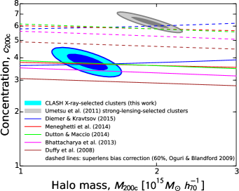
Figure 26: Stacked lensing constraints on the $c$–$M$ relation derived assuming spherical NFW halos for the CLASH X-ray-selected subsample (Umetsu et al., 2016, $c_{\mathrm{200c}}=3.76^{+0.29}_{-0.27}$ at $z_{l}\approx 0.34$; blue contours) and for the superlens sample of Umetsu et al. (2011a, $c_{\mathrm{200c}}=6.31\pm 0.35$ at $z_{l}\approx 0,32$; gray contours). Both results are based on their respective strong and weak lensing analyses. For each case, the contours show the $68.3\%$ and $95.4\%$ confidence levels. The results are compared to theoretical $c$–$M$ relations (solid lines) from numerical simulations of $\mathrm{\Lambda}$CDM cosmologies (Duffy et al., 2008; Bhattacharya et al., 2013; Dutton and Macciò, 2014; Meneghetti et al., 2014; Diemer and Kravtsov, 2015), all evaluated at $z=0.32$ for the full population of halos. The dashed lines show 60% superlens corrections to the solid lines, accounting for the effects of strong-lensing selection and orientation bias expected for the population of superlens clusters (Oguri and Blandford, 2009). Image reproduced with permission from Umetsu et al. (2016), copyright by AAS.

As a precursor study of the CLASH survey, Umetsu et al. (2011a) carried out a combined strong- and weak-lensing analysis of four superlens clusters of similar masses (A1689, A1703, A370, and Cl0024$+$1654; see Umetsu et al., 2011b) using strong-lensing, weak-lensing shear and magnification measurements obtained from high-quality HST and Subaru observations. The stacked sample has a lensing-weighted mean redshift of $z_{l}\approx 0.32$. These clusters display prominent strong-lensing features characterized by large Einstein radii, $\theta_{\mathrm{Ein}}\lower 2.15277pt\hbox{$\;\buildrel>\over{\sim}\;$}30$ arcsec for $z_{s}=2$. Umetsu et al. (2011a) found that the stacked $\langle\!\langle\Sigma\rangle\!\rangle$ profile of the four clusters in the range $R\in[40,2800]h^{-1}\mathrm{kpc}$ is well described by a single NFW profile, with an effective concentration of $c_{\mathrm{200c}}=6.31\pm 0.35$ at $M_{\mathrm{200c}}=(13.4\pm 0.9)\times 10^{14}h^{-1}M_{\odot}$, corresponding to an Einstein radius of $\vartheta_{\mathrm{Ein}}\approx 36$ arcsec for $z_{s}=2$. After applying a 50% superlens correction, Umetsu et al. (2011a) found a discrepancy of $\sim 2\sigma$ with respect to the $c$–$M$ relation of Duffy et al. (2008) calibrated for the WMAP five-year cosmology. They concluded that there is no significant tension between the concentrations of the four clusters and those of $\mathrm{\Lambda}$CDM halos if lensing biases are coupled to a sizable intrinsic scatter in the $c$–$M$ relation.

In Fig. 26, we show in the $c_{\mathrm{200c}}$–$M_{\mathrm{200c}}$ plane the stacked lensing constraints obtained for the CLASH X-ray-selected subsample (Umetsu et al., 2016) and those for the superlens sample of Umetsu et al. (2011a). The stacked lensing constraints for the two cluster samples are compared to theoretical $c$–$M$ relations of Duffy et al. (2008), Bhattacharya et al. (2013), Dutton and Macciò (2014), Meneghetti et al. (2014), and Diemer and Kravtsov (2015, their mean relation), all evaluated for the full population of halos at $z=0.32$. This comparison demonstrates that $c$–$M$ relations that are calibrated for more recent simulations and $\mathrm{\Lambda}$CDM cosmologies (WMAP seven- and nine-year cosmologies and Planck cosmologies) provide better agreement with the CLASH lensing measurements (Umetsu et al., 2014, 2016; Merten et al., 2015). This is also in line with the findings of Dutton and Macciò (2014), who showed that the $c$–$M$ relation in the WMAP five-year cosmology has a 20% lower normalization at $z=0$ than in the Planck cosmology, which has a correspondingly higher normalization in terms of $\mathrm{\Omega}_{\mathrm{m}}$ and $\sigma_{8}$.

To account for the superlens bias in the Umetsu et al. (2011a) sample, Fig. 26 shows each of the $c$–$M$ predictions with a maximal 60% correction applied (Oguri and Blandford, 2009). We see from the figure that, once the effects of selection and orientation bias are taken into account, the results of Umetsu et al. (2011a) come into line with the models of Dutton and Macciò (2014), Meneghetti et al. (2014), and Diemer and Kravtsov (2015), the three most recent $c$–$M$ models studied in Umetsu et al. (2016). Hence, the discrepancy found by Umetsu et al. (2011a) can be fully reconciled by the higher normalization of the $c$–$M$ relation as favored by more recent WMAP and Planck cosmologies (Komatsu et al., 2011; Hinshaw et al., 2013; Planck Collaboration et al., 2016b). Therefore, there appears to be no compelling evidence for the overconcentration problem within the standard $\mathrm{\Lambda}$CDM framework (see also Oguri et al., 2012; Foëx et al., 2014; Robertson et al., 2020).

Another issue when comparing to theoretical relations is that they are generally quantified by the mean and median concentration of individual halos (Diemer and Kravtsov, 2015), rather than that of stacked density profiles (Child et al., 2018). Since the lensing signal depends nonlinearly on halo concentration, even if $c_{\mathrm{200c}}(M_{\mathrm{200c}})$ is normally distributed, there is no guarantee that the concentration extracted from a stacked lensing profile would be equal to the mean of the concentrations of the halos in the stack. The difference can be significant especially when taking into account different stacking procedures used in lensing measurements (Umetsu and Diemer, 2017).

It is intriguing to note that, as already discussed in Sect. 4.3.1, full triaxial modeling of Abell 1689 ($z_{l}=0.183$) shows that combined lensing, X-ray, and SZE observations of the cluster can be consistently explained by its intrinsically high mass concentration combined with a chance alignment of its major axis with the line-of-sight direction (Umetsu et al., 2015). A careful interpretation of lensing, dynamical, and X-ray data based on $N$-body/hydrodynamical simulations suggests that Cl0024$+$1654 ($z_{l}=0.395$) is the result of a high-speed, line-of-sight collision of two massive clusters viewed approximately $2$–$3$ Gyr after impact when the gravitational potential has had time to relax in the center, but before the gas has recovered (Umetsu et al., 2010). Similar to the case of Cl0024$+$1654, Abell 370 ($z_{l}=0.375$) is faint in both X-ray and SZE signals and does not follow the X-ray/SZE observable–mass-scaling relations (see Czakon et al., 2015). $N$-body/hydrodynamical simulations constrained by lensing, dynamical, X-ray, and SZE observations suggest that Abell 370 is a post major merger after the second core passage in the infalling phase, just before the third core passage (Molnar et al., 2020). In this post-collision phase, the gas has not settled down in the gravitational potential well of the cluster, which explains why A370 does not follow the mass scaling relations. Note that, because of its large projected mass and high lensing magnification capability, Abell 370 has been selected as one of the six Hubble Frontier Fields clusters (Lotz et al., 2017).

Finally, it should be noted that high-magnification-selected clusters at $z_{l}>0.5$, such as those selected by the CLASH and Frontier Fields surveys, often turn out to be dynamically disturbed, highly massive ongoing mergers (e.g., Torri et al., 2004; Zitrin and Broadhurst, 2009; Merten et al., 2011; Zitrin et al., 2013; Medezinski et al., 2013, 2016). These ongoing mergers can produce substructured, highly elongated lenses in projection of the sky (e.g., Umetsu et al., 2005; Acebron et al., 2019), enhancing the lensing efficiency (Meneghetti et al., 2003, 2007; Redlich et al., 2012) by boosting the number of multiple images per critical area, due to the increased ratio of the caustic area relative to the critical area (Zitrin et al., 2013). The projected mass distributions of such ongoing mergers cannot be well described by a single NFW profile. In contrast to the superlens clusters at $z_{l}<0.4$ (Umetsu et al., 2011a), NFW fits to the lensing profiles of high-magnification CLASH clusters yield relatively low concentrations (see Umetsu et al., 2016).

6.3 Splashback radius

In the standard $\mathrm{\Lambda}$CDM paradigm of hierarchical structure formation, galaxy clusters form through accretion of matter along surrounding filamentary structures, as well as through successive mergers of smaller objects. An essential picture of halo assembly is that shells of matter surrounding an overdense region in the early universe will initially expand with the Hubble flow, decelerate, turn around, and fall back in. Each shell will cross previously collapsed shells that are oscillating in the growing halo potential. In this picture, accreting particles will pile up near the apocenter of their first orbit, thus creating a sharp density enhancement or caustic in the halo outskirts (Fillmore and Goldreich, 1984; Bertschinger, 1985). This steepening feature depends on the slope of the initial mass perturbation, which determines the mass accretion rate of dark matter halos (Fillmore and Goldreich, 1984; Lithwick and Dalal, 2011). This is illustrated in Fig. 27.

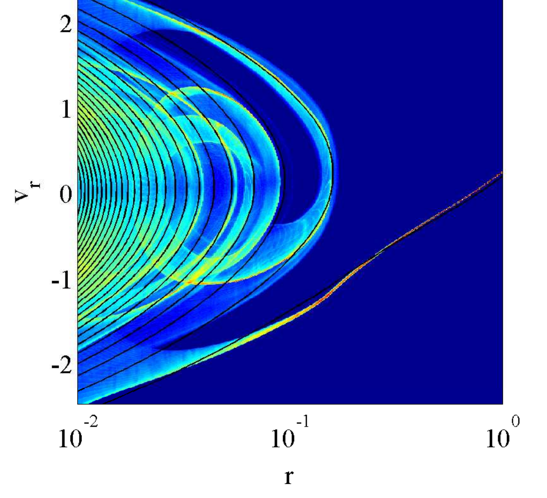
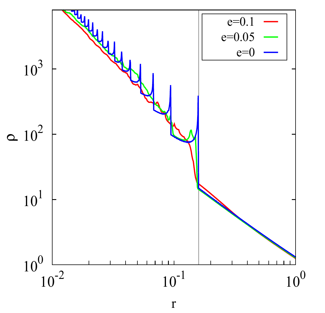
Figure 27: Density caustics for self-similar collisionless halos with an accretion rate of $s=d\ln{M}/d\ln{a}=3$ (Fillmore and Goldreich, 1984; Lithwick and Dalal, 2011). The left panel shows particle trajectories in the phase space diagram for spherically symmetric collapse (solid black curve) and for three-dimensional triaxial collapse (color map). The horizontal axis is the halo-centric distance ($r$) and the vertical axis is the radial velocity ($V_{r}$). The right panel shows the spherically averaged density profile $\rho(r)$ for different values of the initial ellipticity parameter $e$ (Lithwick and Dalal, 2011). The vertical line indicates the location of the outermost caustic, or the splashback radius, predicted by the similarity solution for spherical collisionless collapse with this value of accretion rate. The caustic location depends on the mass accretion rate of halos, while the steepening caustic feature in the spherically averaged $\rho(r)$ depends on $e$. Image reproduced with permission from Adhikari et al. (2014), copyright by IOP and SISSA. See also Shi (2016) for an analytical approach to modeling the outer profile of dark matter halos.

Recently, a closer examination of the halo density profiles in cosmological $N$-body simulations has revealed systematic deviations from the NFW and Einasto profiles in the outskirts at $r\lower 2.15277pt\hbox{$\;\buildrel>\over{\sim}\;$}0.5r_{\mathrm{200m}}$ (Diemer and Kravtsov, 2014). In particular, the halo profiles exhibit a sharp drop in density, a feature associated with the orbital apocenter of the recently accreted matter in the growing halo potential (see Fig. 27). The location of the outermost density caustic expected in collisionless halos is referred to as the splashback radius (Diemer and Kravtsov, 2014; Adhikari et al., 2014; More et al., 2015). The splashback radius constitutes a physical boundary of halos because it sharply separates (at least in perfect spherical symmetry) the multistream intra-halo region from the outer infall region (Diemer and Kravtsov, 2014; More et al., 2015; Mansfield et al., 2017; Okumura et al., 2018). The splashback radius is also related to the transition scale between the 1-halo and 2-halo regimes of the halo–mass correlation function (Garcia et al., 2020).

Splashback features are determined by the orbits of dark matter particles in the halo potential and thus fully characterized in phase space (Diemer, 2017; Okumura et al., 2018). Hence, the steepening feature in the density profile alone cannot capture the full dynamical information of dark matter halos (see Okumura et al., 2018). In particular, the “true” location of the splashback radius based on particle orbits is not equivalent to a particular location in the spherically averaged density profile (Diemer, 2017; Diemer et al., 2017). Nevertheless, it is convenient to define the splashback radius $r_{\mathrm{sp}}$ as the halo radius where the logarithmic slope of the three-dimensional density profile, $\gamma_{\mathrm{3D}}(r)=d\ln{\rho}(r)/d\ln{r}$, is steepest (Diemer and Kravtsov, 2014; More et al., 2015). The splashback radius is a genuine prediction of the standard CDM picture of structure formation. We can possibly learn something about the nature of dark matter and cosmology (Adhikari et al., 2018; Banerjee et al., 2020). Moreover, this steepening feature may be used to make the connection to the dynamical relaxation state of halos.

In the context of $\mathrm{\Lambda}$CDM, the location of $r_{\mathrm{sp}}$ with respect to $r_{\mathrm{200m}}$ is predicted to decrease with mass accretion rate $s(a)\equiv d\ln{M_{\mathrm{vir}}(a)}/d\ln{a}$ (Diemer and Kravtsov, 2014; Adhikari et al., 2014; More et al., 2015; Diemer et al., 2017) and to increase with $\mathrm{\Omega}_{\mathrm{m}}(a)\equiv\overline{\rho}(a)/\rho_{\mathrm{c}}(a)$ (More et al., 2015; Diemer et al., 2017), with some additional dependence on peak height $\nu$ (see Diemer et al., 2017). In $\mathrm{\Lambda}$CDM cosmologies, fast accreting halos have $r_{\mathrm{sp}}\lower 2.15277pt\hbox{$\;\buildrel<\over{\sim}\;$}r_{\mathrm{200m}}$ with a sharper splashback feature, while for slowly accreting halos $r_{\mathrm{sp}}$ can be as large as $(2-3)r_{\mathrm{200m}}$ (More et al., 2015; Diemer et al., 2017). The steepening splashback signal is thus expected to be strongest for massive galaxy clusters because they are, on average, fast accreting systems (Adhikari et al., 2014; Diemer and Kravtsov, 2014). Galaxy clusters are thus the best objects to look for the splashback feature.

The steepening feature near the splashback radius $r_{\mathrm{sp}}$ can be inferred from weak lensing and density statistics of the galaxy distribution. When using galaxies as a tracer of the mass distribution around clusters, however, one needs to account for the effect of dynamical friction that acts to reduce the orbital apocenter of sufficiently massive subhalos hosting cluster galaxies (see Adhikari et al., 2016). Since the efficiency of dynamical friction increases with the ratio of subhalo to cluster halo mass, the impact of dynamical friction on the splashback feature is expected to depend on the luminosity of tracer galaxies (e.g., More et al., 2016; Chang et al., 2018). The splashback feature in stacked galaxy surface density profiles has been routinely detected using cluster–galaxy cross correlations, thanks to statistical samples of clusters defined from large optical or SZE surveys (More et al., 2016; Baxter et al., 2017; Chang et al., 2018; Shin et al., 2019; Zürcher and More, 2019; Murata et al., 2020).

Cluster–galaxy weak lensing can be used to directly test detailed predictions for the splashback feature in the outer density profile of cluster halos. Since the location of the steepest slope in three dimensions is a trade-off between the steepening 1-halo term and the 2-halo term, one needs to precisely measure the lensing signal in both 1-halo and 2-halo regimes spanning a wide range in cluster-centric radius. The location of the three-dimensional splashback radius $r_{\mathrm{sp}}$ can then be inferred by forward-modeling the projected lensing profile ($\Delta\Sigma(R)$ or $\Sigma(R)$) assuming a flexible fitting function, such as the DK14 profile (Sect. 4.3.3). As discussed in More et al. (2016) and Umetsu and Diemer (2017), one would apply two requirements to claim a detection of the splashback radius using a DK14 model (Eq. (130)), namely (1) that the location of the steepest slope in three dimensions can be identified at high statistical significance and (2) that this steepening is greater than expected from a model without a steepening feature, such as an Einasto profile (or a DK14 model with $f_{\mathrm{trans}}(r)=1$). The second criterion is important to ensure that the steepening is associated with a density caustic rather than the transition between the 1-halo and 2-halo terms.

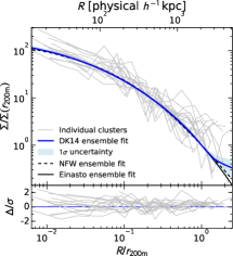
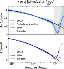
Figure 28: An overview of the first attempt to detect $r_{\mathrm{sp}}$ from lensing (Umetsu and Diemer, 2017). Left: The top panel shows the scaled surface mass density $\Sigma/\Sigma(r_{\mathrm{200m}})$ of the CLASH X-ray-selected sample as a function of $R/r_{\mathrm{200m}}$. The blue thick solid line and the blue shaded area show the best-fit DK14 profile and its $1\sigma$ uncertainty derived from a simultaneous ensemble fit to the scaled $\Sigma$ profiles of 16 individual clusters (gray lines). The corresponding NFW (black dashed) and Einasto (black solid) fits are also shown. The lower panel shows deviations (in units of $\sigma$) of the observed cluster profiles from the best-fit DK14 profile. Right: similarly, the top panel shows the logarithmic gradient of the inferred three-dimensional density profiles as a function of $r/r_{\mathrm{200m}}$ for the DK14, NFW, and Einasto models. The gray vertical shaded area indicates the range from the $16$th to the $84$th percentile of the marginalized posterior distribution of the splashback radius $r_{\mathrm{sp}}/r_{\mathrm{200m}}$. The bottom panel is the same as the top panel, but showing the logarithmic slope of the surface mass density profiles. The best-fit DK14 profile is shown as blue dots at the locations of the data points. This is a slightly modified version of the figure presented in Umetsu and Diemer (2017).

Umetsu and Diemer (2017) were the first to attempt to place direct constraints on the splashback radius $r_{\mathrm{sp}}$ around clusters by using gravitational lensing observations. They developed methods for modeling averaged cluster lensing profiles scaled to a chosen halo overdensity $\Delta$, which can be optimized for the extraction of gradient features that are local in cluster radius, in particular the density steepening due to the splashback radius. Umetsu and Diemer (2017) examined the ensemble mass distribution of 16 CLASH X-ray-selected clusters with a weighted mean mass of $M_{\mathrm{200m}}\approx 13\times 10^{14}h^{-1}M_{\odot}$, by forward-modeling the $\Sigma(R)$ profiles of individual clusters (Fig. 22) obtained by Umetsu et al. (2016). The maximum radius of their ensemble analysis is $R_{\mathrm{max}}\approx 5h^{-1}\mathrm{Mpc}\sim 2.5r_{\mathrm{200m}}$. Their results are shown in Fig. 28. They found that the CLASH ensemble mass profile in projection is remarkably well described by an NFW or Einasto density profile out to $R\approx 1.2r_{\mathrm{200m}}$ (Sect. 6.1), beyond which the data exhibit a flattening with respect to the NFW or Einasto profile due to the 2-halo term. The gradient feature in the cluster outskirts is most pronounced for a scaling with $r_{\mathrm{200m}}$, which is consistent with simulation results of Diemer and Kravtsov (2014) and Lau et al. (2015) (Sect. 6.1). Umetsu and Diemer (2017), however, did not find statistically significant evidence for the existence of $r_{\mathrm{sp}}$ in the CLASH lensing data, as limited by the field of view of Suprime-Cam ($34\times 27$ arcmin²) on the Subaru telescope. Assuming the DK14 profile form and generic priors calibrated with numerical simulations, they placed an informative lower limit on the splashback radius of the clusters, if it exists, of $r_{\mathrm{sp}}/r_{\mathrm{200m}}>0.89$ at $68\%$ confidence. This constraint is in agreement with the $\mathrm{\Lambda}$CDM expectation for the CLASH sample, $r_{\mathrm{sp}}/r_{\mathrm{200m}}\approx 0.97$ (More et al., 2015).

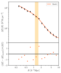
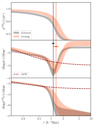
Figure 29: The first successful $r_{\mathrm{sp}}$ determination from weak lensing by Chang et al. (2018). Left: The top panel shows the stacked $\langle\!\langle\Delta\Sigma_{+}\rangle\!\rangle$ profile as a function of (comoving) cluster-centric radius $R$ (black points with error bars) derived for a sample of $3684$ redMaPPer clusters ($0.2<z_{l}<0.55$; $20<\lambda<100$) in the first-year DES data. The red line shows the model fit to the lensing measurements. The inferred location of the splashback radius $r_{\mathrm{sp}}$ with its $1\sigma$ uncertainty is marked by the vertical orange band. The bottom panel shows the residual in the fits divided by the uncertainty of the measurement. Right: comparison of model-fits from the projected galaxy distribution (gray) and weak lensing (red). The upper panel shows the fraction of the density profile $\rho^{\mathrm{coll}}(r)/\rho(r)$ for the collapsed material $\rho^{\mathrm{coll}}(r)\equiv\rho_{\mathrm{E}}(r)f_{\mathrm{trans}}(r)$ over the total density profile $\rho(r)$ (see Eq. (130)). The middle panel shows the logarithmic gradient of the total density profile compared to that of an NFW profile (dashed line). The lower panel shows the logarithmic gradient of the profile for the collapsed material compared to that of an NFW profile. The vertical lines mark the mean values of $r_{\mathrm{sp}}$ inferred from the model fits for both galaxy and lensing measurements, while the horizontal bars in the middle panel indicate the uncertainties on $r_{\mathrm{sp}}$. Image reproduced with permission from Chang et al. (2018), copyright by AAS.

The first successful determination of $r_{\mathrm{sp}}$ from lensing was achieved by Chang et al. (2018), who measured both galaxy number density ($\Sigma_{\mathrm{g}}$) and tangential shear ($\Delta\Sigma_{+}$) profiles around a statistical sample of clusters detected by the red-sequence Matched-filter Probabilistic Percolation (redMaPPer; Rykoff et al., 2016) algorithm in the first year DES data. Their fiducial sample of 3684 clusters is defined by a redshift selection of $0.2<z_{l}<0.55$ and a richness selection of $20<\lambda<100$. The sample is characterized by an effective mass of $M_{\mathrm{200m}}\approx 1.8\times 10^{14}h^{-1}M_{\odot}$ at a mean redshift of $z_{l}\approx 0.41$. The left panels of Fig. 29 show the stacked $\langle\!\langle\Delta\Sigma_{+}(R)\rangle\!\rangle$ profile around their fiducial sample along with the best-fit DK14 profile. For DK14 modeling of the weak-lensing signal (see Sect. 4.3.3), Chang et al. (2018) assumed uniform priors on $(\rho_{-2},r_{-2},b_{\mathrm{e}}\overline{\rho},s_{\mathrm{e}})$ and Gaussian priors on the shape parameters of $\log_{10}{\alpha_{\mathrm{E}}}=\log_{10}(0.19)\pm 0.1$, $\log_{10}{\beta}=\log_{10}(6.0)\pm 0.2$, and $\log_{10}{\gamma}=\log_{10}(4.0)\pm 0.2$ (More et al., 2016; Umetsu and Diemer, 2017), allowing a representative range of values calibrated by $N$-body simulations (Diemer and Kravtsov, 2014; More et al., 2015). They also marginalized over two additional parameters describing the cluster miscentering effect expected for optically selected clusters (Johnston et al., 2007).

With the stacked DES weak-lensing measurements, Chang et al. (2018) constrained the location of the steepest slope in the three-dimensional density profile to lie in the range $r_{\mathrm{sp}}/r_{\mathrm{200m}}=0.97\pm 0.15$. The location and steepness of this gradient feature inferred from the weak-lensing signal agrees within the errors with those inferred from the stacked galaxy density measurements ($r_{\mathrm{sp}}/r_{\mathrm{200m}}=0.82\pm 0.05$), as shown in the right panels of Fig. 29. Note that, as mentioned above, the $r_{\mathrm{sp}}$ determined by the galaxy density profile is expected to be smaller than that of the underlying matter distribution because of dynamical friction, depending on the mass of the galaxies used. From the weak-lensing (or galaxy density) profile, Chang et al. (2018) found the total cluster density profile at the location of $r_{\mathrm{sp}}$ to be steeper than the NFW profile form at a significance level of $2.0\sigma$ (or $3.0\sigma$). Similarly, they found the 1-halo term of the DK14 profile $\rho_{\mathrm{E}}(r)f_{\mathrm{trans}}(r)$ at the location of $r_{\mathrm{sp}}$ to be steeper than the NFW form at the $2.9\sigma$ (or $4.6\sigma$) level.

Chang et al. (2018) found that $r_{\mathrm{sp}}$ measured from weak lensing is smaller than but consistent with the expectation from $N$-body simulations within the large errors. The $r_{\mathrm{sp}}$ measured from the galaxy density profile with a higher precision is significantly smaller than that determined from the corresponding population of subhalos in $N$-body simulations (see also Shin et al., 2019), which is in agreement with the previous results based on the SDSS redMaPPer samples (More et al., 2016; Baxter et al., 2017). Using $N$-body simulations, Chang et al. (2018) found that the effect of dynamical friction is significant only for very massive subhalos and the fiducial galaxy sample used in their analysis is likely not significantly affected by dynamical friction. This discrepancy is likely due to the systematic effects associated with the optical cluster finding algorithm (Zu et al., 2017; Busch and White, 2017; Murata et al., 2020). By analyzing synthetic galaxy catalogs created from $N$-body simulations, Murata et al. (2020) found that the level of systematic bias in the inferred location of $r_{\mathrm{sp}}$ can be significantly alleviated when increasing the aperture size of optical cluster finders beyond the splashback feature.

More recently, Contigiani et al. (2019) placed a stacked lensing constraint on the splashback feature for their sample of 27 high-mass clusters at $0.15<z_{l}<0.55$ targeted by the CCCP survey (Cluster Canadian Comparison Project; Hoekstra et al., 2015). The cluster sample is characterized by a weighted mean mass of $M_{\mathrm{200m}}\approx 12\times 10^{14}h^{-1}M_{\odot}$ at a mean redshift of $z_{l}\sim 0.2$. Their analysis is based on wide-field weak-lensing data taken with CFHT/MegaCam with a $1$ deg² field of view. Their data set is very similar in nature to the CLASH sample of Umetsu and Diemer (2017) because both studies are based on targeted lensing observations of similarly high-mass clusters. Although they did not detect a significant steepening, Contigiani et al. (2019) constrained the splashback radius for their stacked sample as $r_{\mathrm{sp}}=3.6^{+1.2}_{-0.7}$ Mpc (comoving) assuming a DK14 profile with generic priors calibrated with numerical simulations. Although the sample size of clusters in Contigiani et al. (2019) is not significantly larger than that of Umetsu and Diemer (2017), the large field-of-view of CFHT/MegaCam allowed them to better constrain the location and steepness of the splashback feature in the cluster outskirts.

These studies represent a first step toward using cluster–galaxy weak lensing and density statistics of the galaxy distribution to examine well-defined predictions for the splashback features from cosmological $N$-body simulations (e.g., Diemer et al., 2017) and to explore the physics associated with the splashback radius of collisionless halos. A significant improvement in the statistical quality of data is expected from ongoing and upcoming wide-field surveys. On the other hand, improved understanding of systematic effects, such as selection bias of observable-selected clusters and projection effects, will be needed to harness the full potential of such high-precision measurements. Furthermore, the use of phase-space statistics will be extremely useful to explore the properties and signatures of dark matter, in particular of dark matter self interactions (More et al., 2016; Okumura et al., 2018).

6.4 Mass calibration for cluster cosmology

Determining the abundance of rare massive galaxy clusters above a given mass threshold provides a powerful probe of cosmological parameters, especially $\mathrm{\Omega}_{\mathrm{m}}$ and $\sigma_{8}$ (e.g., Rosati et al., 2002). This constraining power is primarily due to the fact that clusters constitute the high-mass tail of hierarchical structure formation, which is exponentially sensitive to the growth of cosmic structure (Haiman et al., 2001; Watson et al., 2014). Conversely, obtaining an accurate calibration of the mass scale for a given cluster sample is key to harness the power of cluster cosmology (Pratt et al., 2019). In this context, large statistical samples of clusters spanning a wide range in mass and redshift, with a well-characterized selection function, provide an independent means of examining any viable cosmological model (e.g., Allen et al., 2004, 2011; Vikhlinin et al., 2009; Mantz et al., 2010; Weinberg et al., 2013; de Haan et al., 2016). In principle, clusters can complement other cosmological probes if the systematics are well understood and controlled.

Thanks to dedicated blind SZE surveys that are made possible in recent years, large homogeneous samples of clusters have been obtained through the SZE selection, out to and beyond a redshift of unity over a wide area of the sky (e.g., Planck Collaboration et al., 2014a, 2016a; Bleem et al., 2015; Hilton et al., 2018). In particular, the Planck satellite mission produced representative catalogs of galaxy clusters detected via the SZE signal from its all-sky survey. The Planck PSZ2 catalog contains 1653 SZE detections of cluster candidates from the 29 month full-mission Planck data (Planck Collaboration et al., 2016a). The full-mission Planck cosmology sample contains $439$ clusters down to S/N of 6, representing the most massive population of clusters with a well-behaved selection function (Planck Collaboration et al., 2016a, c).

Despite these recent advances, we must reiterate that accurate cluster mass measurements are essential in the cosmological interpretation of the cluster abundance (Pratt et al., 2019). Since clusters are detected by the observable baryonic signature, an external calibration of the corresponding observable–mass scaling relation is necessary for a cosmological interpretation of the cluster sample, by accounting for inherent statistical effects and selection bias (e.g., Battaglia et al., 2016; Miyatake et al., 2019; Sereno et al., 2020). This was acutely demonstrated as an internal tension in the Planck analyses (Planck Collaboration et al., 2014b, 2016c), which revealed a non-negligible level of discrepancy between the cosmological parameters $(\mathrm{\Omega}_{\mathrm{m}},\sigma_{8})$ derived from the Planck cluster counts and those from combining the Planck primary CMB measurements with non-cluster data sets, both within the framework of the standard $\mathrm{\Lambda}$CDM cosmology. Here it should be noted that Planck Collaboration et al. (2014b) employed X-ray observations with XMM-Newton to calibrate the scaling relation between the SZE signal strength and cluster mass for their Planck cluster cosmology sample. However, the determination of cluster mass relied on the assumption that the intracluster gas is in hydrostatic equilibrium (hereafter HSE) with the gravitational potential dominated by dark matter.

To characterize the overall level of mass bias (assumed to be constant in cluster mass and redshift) for their SZE-selected clusters, Planck Collaboration et al. (2014b) introduced a parameter defined as (see also Planck Collaboration et al., 2016c):

$$1-b=\left\langle\frac{M_{\mathrm{SZE}}}{M_{\mathrm{true}}}\right\rangle,$$ (169)

where $M_{\mathrm{SZE}}$ denotes the SZE mass proxy and $M_{\mathrm{true}}$ is the true mass (see Penna-Lima et al., 2017), both defined at an overdensity of $\Delta_{\mathrm{c}}=500$. Note that this factor includes not only astrophysical biases but also all systematics encoded in the statistical relationship between the Planck-based mass and the true mass (see Planck Collaboration et al., 2014b; Donahue et al., 2014). The Planck team initially adopted $1-b=0.8$ as a fiducial value with a flat prior in the range $[0.7,1.0]$ (Planck Collaboration et al., 2014b), which is about the level expected due to deviations from the assumed HSE, $b\sim(10-20)\%$ (e.g., Nagai et al., 2007; Meneghetti et al., 2010b; Angelinelli et al., 2020). If the bias were zero, the Planck CMB cosmology would predict far more massive clusters than observed. By analyzing the Planck cosmology sample from the full PSZ2 cluster catalog, Planck Collaboration et al. (2016c) found that the level of mass bias required to bring the Planck cluster counts and Planck primary CMB into full agreement in their base $\mathrm{\Lambda}$CDM cosmology is $1-b=0.58\pm 0.04$. Intriguingly, this would imply that Planck masses underestimate the true values by $b=(42\pm 4)\%$, compared to $b\sim 20\%$ initially adopted by Planck Collaboration et al. (2014b). The level of disagreement between the Planck cluster counts and Planck primary CMB is about $2\sigma$.

While this tension could potentially reflect a higher-than-expected sum of neutrino masses or more exotic physics, the confidence in such a scenario would be limited by systematic uncertainties arising from both astrophysical and observational effects (e.g., Planck Collaboration et al., 2014b; Donahue et al., 2014; Sereno and Ettori, 2017). In fact, the level of disagreement appears to slightly decrease after accounting for updated lower values of the reionization optical depth (Planck Collaboration et al., 2016d). Nevertheless, this tension has attracted considerable attention in the cluster community and led to deeper investigations into the mass calibration for this representative cosmology sample of Planck clusters.

Weak gravitational lensing offers a direct probe of the cluster mass distribution. Cluster–galaxy weak lensing can provide an unbiased mass calibration of galaxy clusters, if one can carefully control systematic effects, such as shear calibration bias (Sect. 3.4.2), photo-$z$ bias, residual cluster contamination (Sect. 4.1), and mass modeling bias (Sect. 4.3). This has become possible thanks to concerted efforts by various groups over the last few decades (e.g., Kaiser et al., 1995; Hoekstra et al., 1998, 2015; Okabe and Umetsu, 2008; Okabe et al., 2010, 2013; Medezinski et al., 2010, 2018b; Oguri, 2010; Umetsu et al., 2011b, 2014; Rosati et al., 2014; von der Linden et al., 2014a; Kelly et al., 2014; Applegate et al., 2014; Merten et al., 2015; Sereno and Ettori, 2015; Melchior et al., 2017; Mandelbaum et al., 2018a, b; Gruen et al., 2019).

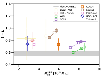
Figure 30: Comparison of $1-b$ as a function of the SZE mass proxy $M_{\mathrm{SZE}}$ for Planck clusters and for clusters detected by the Atacama Cosmology Telescope Polarimeter (ACTpol) experiment. The data points show the ratios of $M_{\mathrm{SZE}}$ to $M_{\mathrm{WL}}$, $1-b_{\mathrm{WL}}=\langle M_{\mathrm{SZE}}/M_{\mathrm{WL}}\rangle$. These $M_{\mathrm{SZE}}$ masses (denoted as $M_{\mathrm{SZ}}^{\mathrm{UPP}}$ in the figure) are derived using the universal pressure profile (UPP) and X-ray mass-scaling relation from Arnaud et al. (2010), which assumes that the intracluster gas is in hydrostatic equilibrium. The gray band indicates the values of $(1-b)$ required to reconcile the Planck cluster counts (Planck Collaboration et al., 2016c) with cosmological parameters from Planck primary CMB (Planck Collaboration et al., 2016b). The blue diamond shows the HSC weak-lensing mass calibration of ACTpol clusters by Miyatake et al. (2019). Previous $(1-b)$ measurements by CS82-ACT (Battaglia et al., 2016), LoCuSS (Smith et al., 2016), CLASH (Penna-Lima et al., 2017), PSZ2LenS (Sereno et al., 2017), and HSC-Planck (Medezinski et al., 2018a) are shown in yellow, brown, orange, pink, and red squares, respectively. The green and purple squares with error bars show the original measurements from the Weighing the Giants project (WtG; von der Linden et al., 2014b) and CCCP (Hoekstra et al., 2015), respectively, and the same colored squares connected by the dashed lines show the $3\%$–$15\%$ range for the Eddington-bias-corrected measurements calculated in Battaglia et al. (2016). Image reproduced with permission from Miyatake et al. (2019), copyright by AAS.

Several recent studies used weak-lensing mass estimates, $M_{\mathrm{WL}}$, to recalibrate cluster masses for subsets of the Planck cosmology sample assuming that the average weak-lensing mass is unbiased (von der Linden et al., 2014b; Hoekstra et al., 2015; Smith et al., 2016; Sereno et al., 2017; Penna-Lima et al., 2017). The samples used in these studies typically contain a few tens of Planck clusters. The results of mass calibrations are controversial in terms of the inferred level of bias, with some studies finding relatively high values of mass bias, $1-b_{\mathrm{WL}}\equiv\langle M_{\mathrm{SZE}}/M_{\mathrm{WL}}\rangle\sim 0.6-0.8$ with typical uncertainties of $\pm 0.1$ (von der Linden et al., 2014b; Hoekstra et al., 2015; Sereno et al., 2017; Penna-Lima et al., 2017), and some finding little bias for low-$z$ Planck clusters, $1-b_{\mathrm{WL}}=0.95\pm 0.04$ (at $0.15<z<0.3$; Smith et al., 2016). However, it should be noted that some of these mass calibrations did not include the correction for Eddington bias and their inferred values of $(1-b_{\mathrm{WL}})$ are thus likely overestimated (see Battaglia et al., 2016; Medezinski et al., 2018a; Miyatake et al., 2019). The results of mass-calibration efforts for SZE-selected cluster samples are summarized in Fig. 30 (for details, see Miyatake et al., 2019).

Recently, Medezinski et al. (2018a) performed a weak-lensing analysis of five Planck clusters located within $\sim 140$ deg² of full-depth and full-color HSC-SSP data. With its unique combination of area and depth, the HSC Wide layer will provide uniformly determined weak-lensing mass measurements for thousands of clusters over the total sky area of $\sim 1000$ deg². This is different from previous studies in which weak-lensing measurements are based on targeted observations and/or archival data. Using the high-quality HSC weak-lensing data and accounting for Eddington bias, Medezinski et al. (2018a) determined the mean level of mass bias to be $1-b_{\mathrm{WL}}=\langle M_{\mathrm{SZE}}/M_{\mathrm{WL}}\rangle=0.80\pm 0.14$ at a mean weak-lensing mass of $M_{\mathrm{WL}}=(4.15\pm 0.61)\times 10^{14}M_{\odot}$. Since Medezinski et al. (2018a) analyzed only five Planck clusters in a lower-mass regime than previous weak-lensing studies, as shown in Fig. 30, this relatively low bias, $b_{\mathrm{WL}}=(20\pm 14)\%$, does not stand in tension with previous higher values of $b_{\mathrm{WL}}$ nor with the level needed to explain the high value of $\sigma_{8}$ found from Planck primary CMB, $b=(42\pm 4)\%$ (Planck Collaboration et al., 2016c).

Therefore, the mystery continues. More representative subsamples with greater overlap with the Planck cosmology sample are needed to draw a definitive conclusion about $(1-b)$ and its cosmological implications. When the full HSC-Wide survey is complete, we expect to have $\sim 40$ Planck clusters observed in the total area of $\sim 1000$ deg². The level of uncertainty on the mass calibration, if assuming it is statistics dominated, will be reduced from the $\sim 10\%$ level achieved with five Planck-HSC clusters (Medezinski et al., 2018a) to reach $\sim 4\%$. This is below the current level of systematic uncertainty in the cluster mass calibration, $\lower 2.15277pt\hbox{$\;\buildrel<\over{\sim}\;$}10\%$ (Medezinski et al., 2018a; Miyatake et al., 2019) and will thus require an even more stringent treatment of weak-lensing systematics. It will also allow us to examine in detail the level of HSE bias and study its possible dependence on cluster mass and redshift, providing valuable information about the thermodynamic history of intracluster gas.

7 Conclusions

In this paper, we presented a comprehensive review of cluster–galaxy weak lensing, covering a range of topics relevant to its cosmological and astrophysical applications. The goals of this review were (1) to provide a self-contained pedagogical overview of the theoretical foundations for gravitational lensing from first principles (Sect. 2), with special attention to the basics and advanced concepts of cluster weak lensing (Sects. 3, 4, and 5), and (2) to summarize and highlight recent advances in our understanding of the mass distribution in and around cluster halos based on numerical simulations and observational results (Sect. 6).

Thanks to concerted community efforts, there has been substantial progress over the last few decades in this area on both observational and theoretical grounds. In this review, we focused on several key issues, namely, the shape of the mass density profile (Sect. 6.1), the $c$–$M$ relation and its intrinsic scatter (Sect. 6.2), splashback features in the cluster outskirts (Sect. 6.3), and cluster mass calibrations for cluster cosmology (Sect. 6.4). Observations of cluster–galaxy weak lensing are, thus far, generally favorable for the standard $\mathrm{\Lambda}$CDM paradigm of structure formation, in terms of the standard explanation for dark matter as effectively collisionless and nonrelativistic on sub-megaparsec scales and beyond, with an excellent match between data and predictions for cluster-size massive halos (Sect. 6).

These studies constitute an encouraging step toward using cluster–galaxy weak lensing to robustly test detailed predictions of $\mathrm{\Lambda}$CDM and its variants, such as SIDM and $\psi$DM, calibrated from cosmological numerical simulations. Such predictions can be unambiguously tested across a wide range in cluster mass and redshift, with large statistical samples of clusters from ongoing and planned lensing surveys, such as Subaru HSC-SSP, DES, LSST, WFIRST, and Euclid.