Graph Classification via Heat Diffusion on Simplicial Complexes

Abstract

In this paper, we study the graph classification problem in vertex-labeled graphs. Our main goal is to classify the graphs comparing their higher-order structures thanks to heat diffusion on their simplices. We first represent vertex-labeled graphs as simplex-weighted super-graphs. We then define the diffusion Fréchet function over their simplices to encode the higher-order network topology and finally reach our goal by combining the function values with machine learning algorithms. Our experiments on real-world bioinformatics networks show that using diffusion Fréchet function on simplices is promising in graph classification and more effective than the baseline methods. To the best of our knowledge, this paper is the first paper in the literature using heat diffusion on higher-dimensional simplices in a graph mining problem. We believe that our method can be extended to different graph mining domains, not only the graph classification problem.

1 Introduction

Graphs (networks) are important structures used to model complex data where nodes (vertices) represent entities and edges represent the interactions or relationships among them aggarwal2010managing ; Cook2006 . We can see the applications of network data in many different areas such as (1) social networks consisting of individuals and their interconnections such as Facebook, coauthorship and citation networks of scientists akbas2017attributed ; akbas2017truss ; tanner2019paper , (2) protein interaction networks from biological networks consisting of proteins that work together to perform some particular biological functions Newman06062006 ; przulj2003graph . Furthermore, we can assign labels to the graph structures such as vertices, edges, or whole graphs. As an example to a vertex-labeled network, in a World Wide Web network of a university, where webpages are vertices and hyperlinks are edges, we can label the nodes as faculty, course, department. As another example, in chemoinformatics, molecules are represented as labeled networks depending on their properties such as anti-cancer activity, molecule toxicity. In addition to labels of each network, vertices, representing atoms, can have labels based on groups of atoms.

Graph classification, as one of many network analysis applications, is the task of identifying the labels of graphs in a graph dataset. It found applications in many different disciplines such as biology borgwardt2005protein , chemistry duvenaud2015convolutional , social network analysis keil2018topological and urban planning bao2017planning . For example, in chemistry, the graph classification task can be detecting labels of graphs, for instance, anti-cancer activity or molecule toxicity.

Although graph classification is practical and essential, there are some challenges of using machine learning algorithms in this task:

1. The enormous sizes of real-world networks make the existing solutions for different graph classification problems hard to adapt with the high computation and space costs.

2. Most current methods only use the vertex and edge information in networks, i.e., only pairwise relations between entities, for classification. However, as we see in different real-world applications, such as human communication, chemical reactions, and ecological systems, interactions can occur in groups of three or more nodes. They cannot be simply described as pairwise relations battiston2020networks .

3. Graph data is complex, and its non-linear structure makes it difficult to apply machine learning algorithms. For example, one cannot use regular measures to compute the similarity between two graphs. These graphs may have a different number of vertices and edges with no clear correspondence.

In this paper, we study the graph classification problem by modeling the higher-order interaction among graphs via heat diffusion on simplicial complexes. While our primary goal in this paper is to address the second challenge of the graph classification using higher-dimensional simplicial complexes, our novel approach also addresses the other challenges as well. Our graph classification model employs the simplex-weighted super-graph representation, heat diffusion on simplicial complexes, and machine learning techniques. We first represent a vertex-labeled graph as a simplex-weighted super-graph with super-nodes being the unique vertex labels. This step compresses the original large graph into a relatively small graph, keeping the crucial information of the original graph as simplex weights in the compressed graph. This scales up the graph classification, hence, addresses the first challenge. Then, we define the heat diffusion not only on vertices (i.e., 0-simplices) but also on higher dimensional simplices such as edges, triangles (i.e., 1-simplices, 2-simplices). We further design the diffusion Fréchet function (DFF) on simplices of the network to extract the higher-order graph topology. DFF is the right choice since it is defined based on the topological and geometrical structure of higher-order graph architecture thanks to the heat diffusion. That is why it allows us to take the higher-order structures in graphs into consideration for the classification problem, hence addresses the second challenge. Applying DFF on a simplex-weighted super-graph will give a value to each super-node in the graph. Then, we create a uniform feature list using the labels of super-nodes for each graph and use DFF values of super-nodes as its features. This feature list provides a clear correspondence between graphs, hence addresses the third challenge. As the last step, we employ machine learning algorithms for classification using these features. We summarize our contributions as follows.

• We design simplex-weighted super-graphs with super-nodes being the unique vertex labels in the vertex-labeled graph. This relatively small graph scales up the graph classification

• We define the heat diffusion on higher dimensional simplices such as edges, triangles and develop the diffusion Fréchet function (DFF) for higher-dimensional simplices to capture the complex structure of the higher-order graph architecture.

• We represent each graph as a vector using the nodes’ labels and their DFF values and use these features for learning.

The paper is structured as follows. In Section 2, we give the necessary background for our method. We first give a formal definition to a network and the graph classification problem, then define simplicial complexes, simplicial Laplacian, and the diffusion Fréchet function on manifolds. We also provide related work in this section. In Section 3, we introduce our graph classification model with explaining our simplex-weighted super-graphs and diffusion Fréchet function on simplicial complexes. In Section 4, we present our experimental results and compare them with the baseline methods. Our final remarks are reported in Section 5.

2 Background

In this section, we discuss the preliminary concepts for networks, graph classification problem, simplicial complexes, and the diffusion Fréchet function (DFF). We also elaborate on related work with a particular focus on the graph classification problem and DFF in graph mining.

2.1 Preliminaries

2.1.1 Networks

In a formal definition, a network $G$ is a pair of sets $G=(V,E)$ where $V$ is the set of vertices and $E\subset V\times V$ is the set of edges of the network. There are various types of networks that represent the differences in the relations between vertices. While in an undirected network, edges link two vertices symmetrically, in a directed network, edges link two vertices asymmetrically. If there is a score for the relationship between vertices that could represent the strength of interaction, it is represented as a weighted network. In a weighted network, a weight function $W:E\rightarrow\mathbb{R}$ on edges is defined to assign a weight for each edge. Furthermore, If vertices of a network have labels, we call these networks as vertex-labeled network. More formally, for a vertex-labeled network, there is a function $l:V\rightarrow L$ defined on vertices that assign a label from the label set $L$ to each vertex.

Graph classification problem is the task of classifying graphs into categories. More formally, given a set of graphs $\mathbb{G}$ and a set of class labels $L$, the graph classification task is to learn a model that maps graphs in $\mathbb{G}$ to the label set $L$.

2.1.2 Simplicial complexes

A simplicial complex $K$ is a finite collection of simplices, i.e., points, edges, triangles, tetrahedron, and higher-dimensional polytopes, such that every face of a simplex of $K$ belongs to $K$ and the intersection of any two simplices of $K$ is a common face of both of them. 0-simplices correspond to vertices, 1-simplices to edges, 2-simplices to triangles, and so on.

Let $S_{p}(K)$ be the set of all $p$-simplices of $K$. An $i$-chain of a simplicial complex $K$ over the field of integers is a formal sum of its $i$-simplices and $i$-th chain group of $K$ with integer coefficients, $C_{i}(K)=C_{i}(K,\mathbb{Z})$, is a vector space over the integer field $\mathbb{Z}$ with basis $S_{i}(K)$. The $i$-th cochain group $C^{i}(K)=C^{i}(K,\mathbb{Z})$ is the dual of the chain group which can be defined by $C^{i}(K):=\text{Hom}(C_{i}(K),\mathbb{Z})$. Here Hom$(C_{i},\mathbb{Z})$ is the set of all homomorphisms of $C_{i}$ into $\mathbb{Z}$. For an $(i+1)$-simplex $\sigma=[v_{0},\dots,v_{i+1}]$, its coboundary operator, $\delta_{i}:C^{i+1}(K)\rightarrow C^{i}(K)$, is defined as

$$(\delta_{i}f)(\sigma)=\sum_{j=1}^{i+1}(-1)^{j}f([v_{0},\dots,\hat{v}_{j},\dots,v_{i+1}]),$$

where $\hat{v}_{j}$ denotes that the vertex $v_{j}$ has been omitted. The boundary operators, $\delta_{i}^{*}$, are the adjoints of the coboundary operators,

$$\cdots C^{i+1}(K)\overset{\delta_{i}}{\underset{\delta_{i}^{*}}{\rightleftarrows}}C^{i}(K)\overset{\delta_{i-1}}{\underset{\delta_{i-1}^{*}}{\rightleftarrows}}C^{i-1}(K)\cdots$$

satisfying $(\delta_{i}a,b)_{C^{i+1}}=(a,\delta_{i}^{*}b)_{C^{i}}$ for every $a\in C^{i}(K)$ and $b\in C^{i+1}(K)$, where $(\cdot,\cdot)_{C^{i}}$ denote the scalar product on the cochain group.

Lastly, we explain how tocreate a simplicial complex from an undirected graph, namely the clique complex.

Definition 1

The clique complex $Cl(G)$ of an undirected graph $G$ is a simplicial complex where vertices of $G$ are its vertices and each $k$-clique, i.e., the complete subgraphs with $k$ vertices, in $G$ corresponds to a $(k-1)$-simplex in $Cl(G)$.

For example, in Figure 1-a, there is a graph with a 4-clique on the left, 2-clique in the middle and 3-clique on the right. Hence, its clique complex, Figure 1-b, has a 3-simplex (tetrahedron), a 1-simplex (edge) and a 2-simplex (triangle).

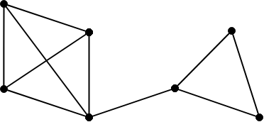
(a) A graph $G$

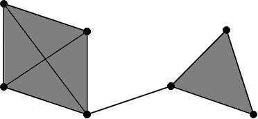
(b) The clique complex $Cl(G)$ of the graph on the left

Figure 1: An example for constructing the clique complex of a graph (borrowed from aktas2019persistence ).

2.1.3 Diffusion Fréchet Function on Manifolds

Originally, Martinez et al. martinez2016multiscale ; martinez2019probing define the diffusion Fréchet function (DFF) on manifolds, and particularly networks, to observe and quantify the local variations on data inspiring from the heat (diffusion) equation. Let $X$ be a compact $C^{\infty}$ manifold in $\mathbb{R}^{n}$. Recall the heat equation PDE

$$\left(\frac{\partial}{\partial t}-\Delta_{X}\right)u=0$$

where the operator $\Delta_{X}$ is the Laplace-Beltrami operator, which is the infinitesimal generator of the heat diffusion process. $\Delta_{X}$ is a self-adjoint, positive semi-definite operator that acts on square integrable functions defined on $X$. Since $X$ is compact, there exists a countable orthonormal basis $\{\phi_{1},\phi_{2},\dots\}$ in the space of the square-integrable functions $\pazocal{L}^{2}(X)$ with real eigenvalues $0\leq\lambda_{1}\leq\lambda_{2}\leq\dots$ such that $\Delta_{X}\phi_{i}=\lambda_{i}\phi_{i}$.

To define DFF on $X$, they first embed each point on $X$ to $\pazocal{L}^{2}(X)$. For each $x\in X$, they associate the function $k_{t}(x,\cdot)=k_{t,x}$ where $k_{t}:X\times X\rightarrow\mathbb{R}$, is the fundamental solution of the heat equation which can be defined as

$$k_{t}(x,y)=\sum_{i=1}^{\infty}e^{-t\lambda_{i}}\phi_{i}(x)\phi_{i}(y).$$ (1)

This function is also called the heat kernel. Here, $k_{t}(x,y)$ can be interpreted as the temperature at time $t$ at point $y$ when the heat source is at the point $x$ at time 0. The larger $k_{t}(x,y)$ means that heat diffuses fast from $x$ to $y$. This is a crucial fact since local geometrical affinities between different points on $X$ can be encoded through this function. For example, if $X$ is a graph with $x$ and $y$ being its vertices, DFF contains information on their connectivity in $X$. The heat kernel can also be seen as a function that describes the topological and geometrical similarity between points points in $X$.

Next, they define the diffusion distance, $d_{t}$, between two points in $X$ as the distance between their functions in $\pazocal{L}^{2}(X)$ with the usual metric of this space, i.e.

$$d_{t}^{2}(x,y)=||k_{t,x}-k_{t,y}||_{\pazocal{L}^{2}(X)}^{2}=\int_{X}(k_{t,x}(z)-k_{t,y}(z))^{2}dz$$ (2)

where $k_{t,x}(\cdot)=k_{t}(x,\cdot)$ for $x\in X$. The main idea here is that if heat diffuses in a similar way from points $x,y\in X$ to any other point $z\in X$, the functions $k_{t,x}$ and $k_{t,y}$ will be close in $\pazocal{L}^{2}(X)$, hence $x$ and $y$ are close in $X$. When we substitute Equation 1 in Equation 2, the diffusion distance can be written as

$$d_{t}^{2}(x,y)=\sum_{k=1}^{n}e^{-2\lambda_{k}t}(\phi_{k}(i)-\phi_{k}(j))^{2}.$$

This distance is robust to noise coifman2006diffusion , which is a crucial fact for using it in data mining problems.

Finally, instead of using the Euclidean distance in the classical Fréchet function, they use the diffusion distance and define the diffusion Fréchet function on manifold as follows.

Definition 2

Let $\alpha$ be some probability measure defined on $X$. The diffusion Fréchet function for manifolds is defined as

$$V_{\alpha,t}:=\int_{X}d_{t}^{2}(x,y)\alpha(dy)=\int_{X}\sum_{k=1}^{n}e^{-2\lambda_{k}t}(\phi_{k}(i)-\phi_{k}(j))^{2}\alpha(dy).$$

To define DFF on the vertices of a network, they first define a heat diffusion process on the network, and for this, they use the Laplacian on vertices. Let $G=(V,E)$ be an undirected, weighted network. The graph Laplacian matrix $\Delta$ is defined by

$$\Delta=D-W$$

where $D$ is the diagonal degree matrix, and $W$ is the weighted adjacency matrix. Then the diffusion Fréchet function on a network can be defined as follows.

Definition 3

Let $\rho=[\rho_{1},\dots,\rho_{n}]^{T}\in\mathbb{R}^{n}$ be a probability distribution on the vertex set $V$ of an undirected weighted network $G$. For $t>0$, the diffusion Fréchet function on vertex $v_{i}$ is defined as

$$F_{\rho,t}(i)=\sum_{j=1}^{n}d_{t}^{2}(i,j)\rho_{j}$$

with

$$d_{t}^{2}(i,j)=\sum_{k=1}^{n}e^{-2\lambda_{k}t}(\phi_{k}(i)-\phi_{k}(j))^{2}$$

where t is the heat diffusion time, $0\leq\lambda_{1}\leq\dots\leq\lambda_{n}$ are the eigenvalues of the graph Laplacian $\Delta$ with orthonormal eigenvectors $\phi_{1},\dots,\phi_{n}$.

Diffusion distance takes manifolds’ and networks’ topological and geometrical structure into consideration. Hence, DFF values provide information on the relative topology of a vertex in the network. In this paper, we extend the diffusion distance to higher-order network structures, namely $p$-th simplices for any $p\geq 0$, beyond the vertices.

2.2 Related work

2.2.1 Graph classification

In literature, there are four main graph classification methods: graph isomorphism zelinka1975certain , graph edit distance bunke2000recent ; blumenthal2020comparing , graph kernels bastiangc ; gkernel ; borgwardt2005protein ; shervashidze2009efficient ; shervashidze2011weisfeiler ; borgwardt2005shortest ; gartner2003graph and graph neural networks errica2019fair ; kernelnn ; zhang2018end . These methods basically measure the similarity between networks by comparing the three network structures in these networks: network topology, vertex weights/attributes, and edge weights/attributes aggarwal2010managing .

In graph isomorphism, one can check whether there is a graph isomorphism or subgraph isomorphism between given two graphs, i.e., match the vertices and edges between these graphs or their subgraphs. Graph edit distances (GED) count graph edit operations, such as node and edge insertion/deletion, that are necessary to transform one graph to another. While GED is very popular for many graph mining problems, exact GED computation is NP-hard. Therefore, many different heuristic algorithms are proposed to compute approximate solutions BORIA202019 ; zeng2009ged ; blumenthal2020comparing ; riesen2009approximate ; kasparged14 . Among them, local search based algorithms zeng2009ged ; BORIA202019 provide the tightest upper bounds for GED.

The graph kernels kriege2020survey ; nikolentzos2019graph , that have attracted a lot of attention during the last decade, are functions employed to handle the non-linear structure of graph data. They are used to measure the similarity between pairs of graphs. One can define kernels using different graph structures such as random walks, shortest paths, and graphlets. Graph kernel methods have high complexity due to a pairwise similarity calculation, which makes it challenging to apply on today’s large graphs. To address the challenges of graph kernels, Graph neural networks have emerged in recent years. Recent methods errica2019fair ; ying2018hierarchical ; morris2019weisfeiler on graph neural networks combine node features and graph topology while extracting the features of the graph for classification. When graphs are noisy or specific sub-networks are essential for the classification, the attention mechanism is used on neural networks lee2018graph .

More recently, persistent homology has been used for graph classification aktas2019persistence ; carriere2019perslay ; zhao2019learning . In these studies, persistent homology is employed to extract the topological features of graphs that persist across multiple scales. The basic idea here is to replace the vertices with a parametrized family of simplicial complexes and encode the change of the topological features (such as the number of connected components, holes, voids) of the simplicial complexes across different parameters aktas2019persistence .

2.2.2 Diffusion Fréchet function in network mining

There are different applications of DFF in network mining problems. The author in martinez2016multiscale studies the co-occurrence networks of microbial communities to analyze the fecal microbiota transplantation in the treatment of C. difficile infection. Besides, in aktas2019classification and aktas2019text , the authors use DFF to classify music networks and text networks respectively. After defining DFF on networks, they use DFF values for classification. Furthermore, in keil2018topological , the authors use the diffusion Fréchet function for the attributed network clustering problem in social networks.

3 Methodology

In this section, we introduce the main parts of our method. We first show how to create simplex-weighted super-graphs from vertex-labeled networks. In the second part, we present how we define the diffusion Fréchet function on simplicial complexes. Finally, we outline our feature extraction and classification methods.

3.1 Simplex-weighted super-graphs

In this paper, we assume that vertices of a network are labeled, i.e., there is a label function $l:V\rightarrow L$ from the vertex set $V$ to a finite label set $L$.

In order to reduce the graph size and create a unified feature list, we first represent a given vertex-labeled network $G=(V,E,l)$ as a compressed super-graph $\mathscr{G}=(\mathscr{V},\mathscr{E})$. It consists of a super-node set, $\mathscr{V}$, and a super-edge set, $\mathscr{E}$; each super-node $\nu\in\mathscr{V}$ represents a unique vertex label of the network, each super-edge $(\nu,\mu)\in\mathscr{E}$ between two super-nodes $(\nu$ and $\mu)$ represents the edge between a vertex with the label $\nu$ and a vertex with the label $\mu$ in the original network. Besides, we define weights on super-nodes and super-edges to reflect the frequency and co-occurrences of labels. We assign weights to super-nodes as the number of the corresponding label occurrences weights to super-edges as the co-occurrence frequency of the labels. The formal definition of our representation is as follows.

Definition 4 (Compressed super-graphs)

Let $G=(V,E,l)$ be a vertex-labeled network with $l:V\rightarrow L$ being the label function and $L$ being the set of unique labels of $V$. Let $\mathscr{G}=(\mathscr{V},\mathscr{E},W_{\mathscr{V}},Y_{\mathscr{E}})$ be the simplex-weighted super-graph of $G$ where $\mathscr{V}$ is the set of super-nodes, $\mathscr{E}$ is the set of super-edges, $W_{V}$ is the set of super-node weights and $Y_{E}$ is the set of super-edge weights. $\mathscr{G}$ is defined as follows

• $\mathscr{V}=\{\nu_{1},\dots,\nu_{n_{L}}|n_{L}\text{ is the size of }L\}$,

• $\mathscr{E}=\{e_{1},\dots,e_{m}|e_{k}=(\nu_{i},\nu_{j})\text{ for }1\leq i,j\leq n_{L},1\leq k\leq m\text{ where }m\text{ is the number}\\ \text{of different co-occurrences of labels in }G\}$,

• $W_{\mathscr{V}}=\{\omega_{1},\dots,\omega_{n_{L}}|\omega_{i}\text{ is the frequency of the label }l_{i}\in L\text{ for }1\leq i\leq n_{L}\}$

• $Y_{\mathscr{E}}=\{y_{1},\dots,y_{m}|y_{k}\text{ is the frequency of the co-occurrence}\text{ of the labels }l_{i},l_{j}\\ \text{ for }1\leq i,j\leq n_{L},1\leq k\leq m\}$,

Furthermore, as the next step, we assign weights on simplices of the super-graph to record the co-occurrence frequency of higher-order structures on graphs.

Definition 5 (Simplex weights)

Let $S_{p}$ be the $p$-simplices of a super-graph $\mathscr{G}$, i.e., $S_{p}=\{\sigma_{1},\dots,\sigma_{n_{p}}|\sigma_{i}=[v_{0},\dots,v_{p}]\in Cl(G)\text{ for }1\leq i\leq n_{p}\text{ where }n_{p}\text{ is the number of }\\ p\text{-cliques in }\mathscr{G}\text{ with }p>1\}$. We define a weight function $z:S_{p}\rightarrow\mathbb{Z}^{+}$ on $S_{p}$ such that for any $\sigma_{i}\in S_{p}$, $z(\sigma_{i})=\text{ min}\{y_{1},\dots,y_{r}\}$ with $r={p+1\choose 2}$, where $y_{j}$’s are the weights of the edges in $\sigma_{i}$.

The weights defined here will be used to define DFF on simplicial complexes in the next section. We close this section with an example of a simplex-weighted super-graph.

Example 1

In Figure 2, we present a simplex-weighted super-graph of a vertex-labeled network in the DD dataset. While the original network has 327 vertices (0-simplices), 1798 edges (1-simplices), and 4490 triangles (2-simplices), its simplex-weighted super-graph has only 19 vertices, 172 edges and 1031 triangles since the original graph has only 19 different vertex labels. The darker vertices and edges have larger weights in Figure 2-(b).

(a) Original network $G$

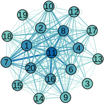
(b) Weighted super-graph $\mathscr{G}$ of $G$ in (a)

Figure 2: Example of our simplex-weighted super-graph representation of a network in the DD dataset. The darker vertices and edges have larger weights in (b).

3.2 Diffusion Fréchet function on simplicial complexes

In this section, we explain how to extend the diffusion Fréchet function to any dimensional simplices beyond the vertices. For this, we first explain the simplicial Laplacian, and then we use it to define DFF on simplicial complexes.

3.2.1 Simplicial Laplacian

As we show in Section 2.1.3, the Laplacian matrix $\Delta$ is used to define the heat diffusion among the vertices of a graph through edges. However, as we explained before, this model is only considers the pairwise relations between vertices and ignores higher-order structures in graphs. In order to model heat diffusion on higher dimensional simplices and extract higher-order structures in graphs, we need to use an analog of the Laplacian matrix $\Delta$ for higher dimensions. In horak2013spectra , the three simplicial Laplacian operators for higher-dimensional simplices, using the boundary and coboundary operators between chain groups, are defined as

$$\pazocal{L}_{p}^{\text{down}}=\delta_{p-1}\delta_{p-1}^{*}\textit{ ~{}~{}~{}~{}~{}~{}~{}~{}~{}~{} down Laplacian~{}~{}}$$

$$\pazocal{L}_{p}^{\text{up}}(K)=\delta_{p}^{*}\delta_{p}\textit{ ~{}~{}~{}~{}~{}~{}~{}~{}~{}~{}~{}~{}~{} up Laplacian~{}~{}~{}~{}~{}}$$

$$~{}\pazocal{L}_{p}(K)=\pazocal{L}_{p}^{\text{up}}+\pazocal{L}_{p}^{\text{down}}\textit{ ~{}~{}~{}~{}~{} Laplacian~{}~{}~{}~{}~{}~{}~{}~{}~{}~{}}$$

These operators are self-adjoint, non-negative, compact and have different spectral properties horak2013spectra .

To make the expression of Laplacian explicit, they identify each coboundary operator $\delta_{p}$ with an incidence matrix $D_{p}$ in horak2013spectra . The incidence matrix $D_{p}\in\mathbb{Z}_{2}^{n_{p+1}}\times\mathbb{Z}_{2}^{n_{p}}$ encodes which $p$-simplices are incident to which $(p+1)$-simplices where $n_{p}$ is number of $p$-simplices. It is defined as

$$D_{p}(i,j)=\left\{\begin{tabular}[]{ll}$1$&if $\sigma_{j}^{p}$ is on the boundary of $\sigma_{i}^{p+1}$\\ $0$&otherwise\end{tabular}\right.$$

Here, we assume the simplices are not oriented. One can incorporate the orientations by simply adding “$D_{p}(i,j)=-1$ if $\sigma_{j}^{p}$ is not coherent with the induced orientation of $\sigma_{i}^{p+1}$” in the definition if needed.

Furthermore, we assume that the simplices are weighted, i.e. there is a weight function $z$ defined on the set of all simplices of $K$ whose range is $\mathbb{R}^{+}$. let $W_{p}$ be an $n_{p}\times n_{p}$ diagonal matrix with $W_{p}(j,j)=z(\sigma_{j}^{p})$ for all $j\in\{1,\dots,n_{p}\}$. Then, the $i$-dimensional up Laplacian can be expressed as the matrix

$$\pazocal{L}_{i}^{\text{up}}=W_{i}^{-1}D_{i}^{T}W_{i+1}D_{i}.$$

Similarly, the $i$-dimensional down Laplacian can be expressed as the matrix

$$\pazocal{L}_{i}^{\text{down}}=D_{i-1}W_{i-1}^{-1}D_{i-1}^{T}W_{i}.$$

Then, to express the $i$-dimensional Laplacian $\pazocal{L}_{i}$, we can add these two matrices.

3.2.2 Diffusion Fréchet function on simplicial complexes

The graph Laplacian used in Definition 3 is the $0$-th dimensional up Laplacian, i.e. $\Delta=D-W=\pazocal{L}_{0}^{\text{up}}$. Hence, in the case of DFF on vertices, we assume that the heat source is on vertices, and heat diffuses between vertices through edges. However, heat diffusion, the diffusion distance, and DFF can also be defined on $p$-simplices using the simplicial Laplacian operators for any $p>0$. In the case of down Laplacian, $\pazocal{L}_{p}^{\text{down}}$, we assume that heat sources are located on $p$-simplices and heat diffuses through $(p-1)$-simplices. In the case of up Laplacian, $\pazocal{L}_{p}^{\text{up}}$, we assume that heat sources are located on $p$-simplices and heat diffuses through $(p+1)$-simplices. In the case of Laplacian, $\pazocal{L}_{p}$, we assume that heat sources are located on $p$-simplices and heat diffuses both through $(p-1)$-simplices and $(p+1)$-simplices.

Moreover, to define DFF on $p$-simplices with $p\geq 0$, we need to define a probability distribution on these simplices. We define a probability distribution on $p$-simplices using the simplex weights as follows.

Definition 6 (Probability distribution on $p$-simplices)

Let $\mathscr{G}=(\mathscr{V},\mathscr{E},\\ W_{\mathscr{V}},Y_{\mathscr{E}})$ be a simplex-weighted super-graph and $S_{p}=\{\sigma_{1},\dots,\sigma_{k}\}$ be its $p$-simplices with weights $z(S_{p})=\{z_{1},\dots,z_{k}\}$. Then the probability distribution $\rho=[\rho_{1},\dots,\rho_{k}]^{T}\in\mathbb{R}^{k}$ is defined as

$$\rho_{i}=\frac{z_{i}}{\sum_{j=1}^{k}z_{j}}$$

for $1\leq i\leq k$.

This definition allows us to make larger weights having more contribution to the diffusion Fréchet function. This fact is crucial since the labels that occur more often in a network can have a vital role in classification.

Using Laplacian on simplicial complexes and probability distribution on $p$-simplices, we can define the diffusion Fréchet function on simplicial complexes as follows.

Definition 7 (DFF on simplicial complexes)

Let $\rho=[\rho_{1},\dots,\rho_{n_{p}}]^{T}\in\mathbb{R}^{n_{p}}$ be a probability distribution on $p$-simplices of a simplicial complex $K$. For $t>0$, the diffusion Fréchet function on a $p$-simplex $\sigma_{i}$ is defined as

$$F_{\rho,t}(i)=\sum_{j=1}^{n_{p}}d_{t}^{2}(i,j)\rho_{j}$$

with

$$d_{t}^{2}(i,j)=\sum_{k=1}^{n_{p}}e^{-2\lambda_{k}t}(\phi_{k}(i)-\phi_{k}(j))^{2}$$

where $0\leq\lambda_{1}\leq\dots\leq\lambda_{n_{p}}$ are the eigenvalues of the Laplacian $\pazocal{L}_{p}$ with orthonormal eigenvectors $\phi_{1},\dots,\phi_{n_{p}}$.

We can define the up diffusion Fréchet function $F_{\mathscr{E},t}^{\text{up}}$ and down diffusion Fréchet function $F_{\mathscr{E},t}^{\text{down}}$ by using the up Laplacian $\pazocal{L}_{p}^{\text{up}}$ and the down Laplacian $\pazocal{L}_{p}^{\text{down}}$ in the definition respectively. All these functions extract the topology and geometry of higher-order graph structures thanks to heat diffusion in different directions.

3.3 Feature extraction and classification

For feature extraction, we first need to define the feature list for networks, and we employ the vertex labels for this sake. For 0-simplices, i.e., vertices, the feature list is the unique vertex labels observed in a given dataset. We first compute DFF on vertices. Then, we assign the reciprocal of that label’s vertex’ DFF value as the corresponding feature for that network. We use the reciprocal of the DFF values as features since the vertices of high degree with larger vertex and edge weights have smaller DFF values. However, these vertices are more critical for networks. Hence they need to have larger feature value to stress their importance. If a label in the feature list is not observed in a network, we assign zero as the corresponding feature. This process provides a feature vector for each network.

For $p$-simplices with $p>0$, such as edges, triangles, we use vertex labels to label simplices and take the feature list as the all different labels of $p$-simplices observed in a given dataset. Then, we compute DFF on these $p$-simplices. As we do in the vertex case, if a label in the feature list is not observed in a network, we assign zero as the corresponding feature for the document. Otherwise, we assign the reciprocal of that label’s simplex’ DFF value as the corresponding feature for that network. This process provides a feature vector for each network for a fixed dimension of $p$.

Furthermore, the scale parameter $t$ in Definition 3 and Definition 7, which is the heat diffusion time as given by definitions, can be considered as the locality index, i.e., the smaller the scale parameter value we use, the more local information on the networks we obtain. We can see the effect of this value in Figure 3. In our experiments, we use different parameter values to understand their impact on classification.

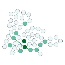
(a) Original network

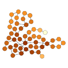
(b) $t=1$

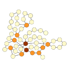
(c) $t=10^{-3}$

Figure 3: Diffusion Fréchet function defined on a weighted network (a) in two different scale parameters (b) $t=1$, and (c) $t=10^{-3}$. While the darker vertices and edges have larger weights in (a), it means smaller diffusion Fréchet function values in (b) and (c) (borrowed from aktas2019text ).

After obtaining the features of each network up to a scale parameter value $t$ in the diffusion Fréchet function, we train a classifier using these features of networks and their class values with a machine learning algorithm.

4 Experiments

In this section, we first introduce the datasets we use in our experiments. Then, we share the classification results for different simplex dimensions and scale parameter values in DFF. Lastly, we compare our method with the baseline graph classification methods.

4.1 Datasets

To test the efficiency of our method, we apply our framework to real-world bioinformatics networks: MUTAG, PROTEINS, PTC, and DD. MUTAG debnath1991structure is a mutagenic nitro compound dataset, including 188 samples with two classes: aromatic and heteroaromatic. Its vertices have seven discrete labels. PROTEINS borgwardt2005protein is a protein-protein interaction network whose vertices are secondary structure elements, and vertices that are neighbors in the amino-acid sequence of in 3D space are connected with an edge. Its vertices have 3 discrete labels, representing helix, sheet or turn. PTC toivonen2003statistical is a dataset of 344 chemical compounds about the carcinogenicity for male and female rats, and its vertices have 19 discrete labels. DD dobson2003distinguishing is a collection of 1,178 protein network structures with 82 discrete vertex labels, where each graph is classified as enzyme or non-enzyme class. Table 1 has a summary of the statistics of these datasets.

Table 1: Properties of the network datasets used in experiments.

Datasets	Size	Classes	Avg. nodes	Avg. edges	Labels
MUTAG	188	2	17.9	19.8	7
PROTEINS	1113	2	39.1	72.9	3
PTC	344	2	14.3	14.7	19
DD	1178	2	284.3	715.7	82

4.2 Results

In our experiments, we compute DFF on vertices, edges, and triangles (i.e., 0-, 1- and 2-simplices). For vertices, we define the heat diffusion only for up Laplacian since down Laplacian is not defined for vertices. For edges, we define the heat diffusion using down Laplacian, up Laplacian, and both. Lastly, we only define down Laplacian for triangles since we only need to compute the 1-dimensional incidence matrix $D_{1}$. Furthermore, we use the simplex weights of $p$-simplices with $p\in\{0,1,2\}$ only in the probability distribution, but not in Laplacian (i.e., we assume $W_{p}$ is the identity matrix in $\pazocal{L}_{p}$), to keep the Laplacian matrix symmetric.

Besides, we use the parameter values $t\in\{1,10^{-1},10^{-2},10^{-3},10^{-4},10^{-5}\}$ to test the efficiency of our method for different parameter values.

After obtaining the feature vector of each network, we apply the Random Forest classification algorithm to build our prediction model. We use the 10-fold cross-validation process to evaluate our method. Finally, we obtain classification results (accuracy) for each dataset and different $t$ values in Table 2.

Table 2: Classification results (accuracy) for different simplex dimensions and scale parameter $t$ values. The cells for the best result in each column for each dataset is colored gray.

		$1$	$10^{-1}$	$10^{-2}$	$10^{-3}$	$10^{-4}$	$10^{-5}$
MUTAG	Vertex-up	81.91	82.98	82.45	82.45	84.04	82.98
	Edge-down	85.64	86.17	86.70	86.17	87.23	86.70
	Edge-up	82.45	84.04	86.70	86.17	87.23	88.30
	Edge-both	84.04	84.04	87.77	88.30	88.30	87.77
	Triangle-down	84.57	84.04	84.04	81.91	82.45	83.51
PROTEINS	Vertex-up	67.20	69.84	76.46	72.75	71.69	69.31
	Edge-down	73.50	73.23	69.81	69.90	70.17	70.89
	Edge-up	72.42	72.42	74.39	71.25	69.90	71.34
	Edge-both	70.44	71.52	74.39	70.89	70.89	70.44
	Triangle-down	74.03	71.70	69.99	69.00	68.64	69.27
PTC	Vertex-up	55.52	58.14	62.79	59.88	59.59	59.59
	Edge-down	61.92	60.47	60.47	62.50	61.05	61.05
	Edge-up	56.98	59.88	62.79	58.43	59.01	56.98
	Edge-both	61.34	60.47	63.66	59.01	59.59	58.43
	Triangle-down	54.65	55.52	54.36	54.94	53.78	54.65
DD	Vertex-up	71.22	76.32	76.91	77.67	79.03	78.35
	Edge-down	75.55	75.89	73.34	71.65	73.43	73.60
	Edge-up	73.26	74.79	76.15	75.98	73.94	72.16
	Edge-both	74.70	75.13	74.28	75.30	74.36	73.17
	Triangle-down	77.67	77.08	77.08	76.40	76.66	76.91

While the best accuracy results are obtained with the heat diffusion on vertices in PROTEINS and DD, the heat diffusion on edges provides the best results in MUTAG and PTC. Furthermore, the heat diffusion on triangles gives the best results in DD for three different $t$ values since the DD dataset has many triangles comparing to other datasets.

Furthermore, the effect of the scale parameter values also changes depending on both dataset and dimension. For example, while the smaller $t$ values increase the accuracy in MUTAG for edges, it decreases the accuracy in PROTEINS and DD for triangles.

4.3 Comparison

We compare our model with the following baseline methods; graphlet kernel (GK) shervashidze2009efficient , Weisfeiler-Lehman kernel (WL) shervashidze2011weisfeiler , shortest-path kernel (SP) borgwardt2005shortest , and random walk kernel (RW) gartner2003graph . The same classification process has been applied with these methods for a fair comparison. The comparison results are in Table 3 and Figure 4. Here, for our each different method, we choose the $t$ values that gives the best results.

As we see in the table and the figure, our method performs better than the baseline methods on MUTAG, PROTEINS, and PTC and performs similar to WL in DD. This clearly indicates that higher-order network features obtained from heat diffusion on simplicial complexes is quite effective in the graph classification problem.

Table 3: Classification rates (accuracy) of the proposed algorithms and the baseline methods. The cells for the best result in each column is colored gray. $>$ 24h indicates that the computation did not finish after 24 hours.

	MUTAG	PROTEINS	PTC	DD
Vertex-up	84.04	76.46	62.79	79.03
Edge-down	87.23	73.50	62.50	75.89
Edge-up	88.30	74.39	62.79	76.15
Edge-both	88.30	74.39	63.66	75.30
Triangle-down	84.57	74.03	55.52	77.67
GK	81.66	71.67	57.26	78.40
WL	80.72	72.92	56.97	79.70
SP	85.22	75.07	58.24	$>$ 24h
RW	83.72	74.22	57.85	$>$ 24h

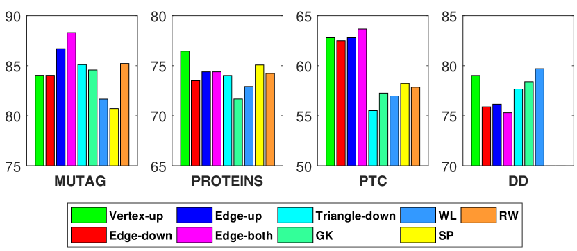
Figure 4: Classification rates (accuracy) of the proposed algorithm and the baseline methods

5 Conclusion

In this paper, we propose a novel method for the graph classification problem. We first represent a vertex-labeled network with a simplex-weighted super-graph. We then define the diffusion Fréchet function over the simplices of the networks to encode their non-trivial relations as the network features. We then classify graphs with the Random Forest classification algorithm and 10-fold cross-validation using these features. We show that the proposed algorithm has better classification results than the baseline methods. This paper is the first study in the literature showing the potential of using heat diffusion on simplicial Laplacians in the graph mining area.

Conflict of interest

The authors declare that they have no conflict of interest.

References

- (1) Aggarwal, C.C., Wang, H.: Managing and mining graph data, vol. 40. Springer (2010)
- (2) Akbas, E., Zhao, P.: Attributed graph clustering: An attribute-aware graph embedding approach. In: Proceedings of the 2017 IEEE/ACM International Conference on Advances in Social Networks Analysis and Mining 2017, pp. 305–308 (2017)
- (3) Akbas, E., Zhao, P.: Truss-based community search: a truss-equivalence based indexing approach. Proceedings of the VLDB Endowment 10(11), 1298–1309 (2017)
- (4) Aktas, M.E., Akbas, E.: Text classification via network topology: A case study on the holy quran. In: 2019 18th IEEE International Conference On Machine Learning And Applications (ICMLA), pp. 1557–1562. IEEE (2019)
- (5) Aktas, M.E., Akbas, E., El Fatmaoui, A.: Persistence homology of networks: methods and applications. Applied Network Science 4(1), 61 (2019)
- (6) Aktas, M.E., Akbas, E., Papayik, J., Kovankaya, Y.: Classification of turkish makam music: a topological approach. Journal of Mathematics and Music 13(2), 135–149 (2019)
- (7) Bao, J., He, T., Ruan, S., Li, Y., Zheng, Y.: Planning bike lanes based on sharing-bikes’ trajectories. In: Proceedings of the 23rd ACM SIGKDD international conference on knowledge discovery and data mining, pp. 1377–1386 (2017)
- (8) Battiston, F., Cencetti, G., Iacopini, I., Latora, V., Lucas, M., Patania, A., Young, J.G., Petri, G.: Networks beyond pairwise interactions: structure and dynamics. arXiv preprint arXiv:2006.01764 (2020)
- (9) Blumenthal, D.B., Boria, N., Gamper, J., Bougleux, S., Brun, L.: Comparing heuristics for graph edit distance computation. The VLDB Journal 29(1), 419–458 (2020)
- (10) Borgwardt, K.M., Kriegel, H.P.: Shortest-path kernels on graphs. In: Fifth IEEE International Conference on Data Mining (ICDM’05), pp. 8–pp. IEEE (2005)
- (11) Borgwardt, K.M., Ong, C.S., Schönauer, S., Vishwanathan, S., Smola, A.J., Kriegel, H.P.: Protein function prediction via graph kernels. Bioinformatics 21(suppl_1), i47–i56 (2005)
- (12) Boria, N., Blumenthal, D.B., Bougleux, S., Brun, L.: Improved local search for graph edit distance. Pattern Recognition Letters 129, 19 – 25 (2020)
- (13) Bunke, H.: Recent developments in graph matching. In: Proceedings 15th International Conference on Pattern Recognition. ICPR-2000, vol. 2, pp. 117–124. IEEE (2000)
- (14) Carriere, M., Chazal, F., Ike, Y., Lacombe, T., Royer, M., Umeda, Y.: Perslay: A neural network layer for persistence diagrams and new graph topological signatures. stat 1050, 17 (2019)
- (15) Coifman, R.R., Lafon, S.: Diffusion maps. Applied and computational harmonic analysis 21(1), 5–30 (2006)
- (16) Cook, D.J., Holder, L.B.: Mining Graph Data. John Wiley & Sons (2006)
- (17) Debnath, A.K., Lopez de Compadre, R.L., Debnath, G., Shusterman, A.J., Hansch, C.: Structure-activity relationship of mutagenic aromatic and heteroaromatic nitro compounds. correlation with molecular orbital energies and hydrophobicity. Journal of medicinal chemistry 34(2), 786–797 (1991)
- (18) Dobson, P.D., Doig, A.J.: Distinguishing enzyme structures from non-enzymes without alignments. Journal of molecular biology 330(4), 771–783 (2003)
- (19) Duvenaud, D.K., Maclaurin, D., Iparraguirre, J., Bombarell, R., Hirzel, T., Aspuru-Guzik, A., Adams, R.P.: Convolutional networks on graphs for learning molecular fingerprints. In: Advances in neural information processing systems, pp. 2224–2232 (2015)
- (20) Errica, F., Podda, M., Bacciu, D., Micheli, A.: A fair comparison of graph neural networks for graph classification. arXiv preprint arXiv:1912.09893 (2019)
- (21) Gärtner, T., Flach, P., Wrobel, S.: On graph kernels: Hardness results and efficient alternatives. In: Learning theory and kernel machines, pp. 129–143. Springer (2003)
- (22) Horak, D., Jost, J.: Spectra of combinatorial laplace operators on simplicial complexes. Advances in Mathematics 244, 303–336 (2013)
- (23) Keil, W., Aktas, M.: Topological data analysis of attribute networks using diffusion frechet function with ego-networks. In: The 7th International Conference on Complex Networks and Their Applications (extended Abstract), Cambridge, United Kingdom, pp. 194–196 (2018)
- (24) Kriege, N.M., Johansson, F.D., Morris, C.: A survey on graph kernels. Applied Network Science 5(1), 1–42 (2020)
- (25) Lee, J.B., Rossi, R., Kong, X.: Graph classification using structural attention. In: Proceedings of the 24th ACM SIGKDD International Conference on Knowledge Discovery & Data Mining, pp. 1666–1674 (2018)
- (26) Martinez, D.H.D.: Multiscale summaries of probability measures with applications to plant and microbiome data. Ph.D. thesis, The Florida State University (2016)
- (27) Martínez, D.H.D., Lee, C.H., Kim, P.T., Mio, W.: Probing the geometry of data with diffusion fréchet functions. Applied and Computational Harmonic Analysis 47(3), 935–947 (2019)
- (28) Morris, C., Ritzert, M., Fey, M., Hamilton, W.L., Lenssen, J.E., Rattan, G., Grohe, M.: Weisfeiler and leman go neural: Higher-order graph neural networks. In: Proceedings of the AAAI Conference on Artificial Intelligence, vol. 33, pp. 4602–4609 (2019)
- (29) Newman, M.J.: Modularity and community structure in networks. Proceedings of the National Academy of Sciences 103(23), 8577–8582 (2006). National Academy of Sciences
- (30) Nikolentzos, G., Meladianos, P., Tixier, A.J.P., Skianis, K., Vazirgiannis, M.: Kernel graph convolutional neural networks. In: V. Kůrková, Y. Manolopoulos, B. Hammer, L. Iliadis, I. Maglogiannis (eds.) Artificial Neural Networks and Machine Learning – ICANN 2018, pp. 22–32. Springer International Publishing, Cham (2018)
- (31) Nikolentzos, G., Siglidis, G., Vazirgiannis, M.: Graph kernels: A survey. arXiv preprint arXiv:1904.12218 (2019)
- (32) Przulj, N.: Graph theory approaches to protein interaction data analysis. Tech. rep., University of Toronto (2004)
- (33) Rieck, B., Bock, C., Borgwardt, K.: A persistent weisfeiler-lehman procedure for graph classification. In: K. Chaudhuri, R. Salakhutdinov (eds.) Proceedings of the 36th International Conference on Machine Learning, Proceedings of Machine Learning Research, vol. 97, pp. 5448–5458. PMLR, Long Beach, California, USA (2019)
- (34) Riesen, K., Bunke, H.: Approximate graph edit distance computation by means of bipartite graph matching. Image and Vision computing 27(7), 950–959 (2009)
- (35) Riesen, K., Fischer, A., Bunke, H.: Combining bipartite graph matching and beam search for graph edit distance approximation. In: N. El Gayar, F. Schwenker, C. Suen (eds.) Artificial Neural Networks in Pattern Recognition, pp. 117–128. Springer International Publishing, Cham (2014)
- (36) Shervashidze, N., Schweitzer, P., Van Leeuwen, E.J., Mehlhorn, K., Borgwardt, K.M.: Weisfeiler-lehman graph kernels. Journal of Machine Learning Research 12(77), 2539–2561 (2011)
- (37) Shervashidze, N., Vishwanathan, S., Petri, T., Mehlhorn, K., Borgwardt, K.: Efficient graphlet kernels for large graph comparison. In: Artificial Intelligence and Statistics, pp. 488–495 (2009)
- (38) Tanner, W., Akbas, E., Hasan, M.: Paper recommendation based on citation relation. In: 2019 IEEE International Conference on Big Data (Big Data), pp. 3053–3059. IEEE (2019)
- (39) Toivonen, H., Srinivasan, A., King, R.D., Kramer, S., Helma, C.: Statistical evaluation of the predictive toxicology challenge 2000–2001. Bioinformatics 19(10), 1183–1193 (2003)
- (40) Yanardag, P., Vishwanathan, S.: Deep graph kernels. In: Proceedings of the 21th ACM SIGKDD International Conference on Knowledge Discovery and Data Mining, KDD ’15, p. 1365–1374. Association for Computing Machinery, New York, NY, USA (2015)
- (41) Ying, Z., You, J., Morris, C., Ren, X., Hamilton, W., Leskovec, J.: Hierarchical graph representation learning with differentiable pooling. In: Advances in neural information processing systems, pp. 4800–4810 (2018)
- (42) Zelinka, B.: On a certain distance between isomorphism classes of graphs. Časopis pro pěstování matematiky 100(4), 371–373 (1975)
- (43) Zeng, Z., Tung, A.K.H., Wang, J., Feng, J., Zhou, L.: Comparing stars: On approximating graph edit distance. Proc. VLDB Endow. 2(1), 25–36 (2009)
- (44) Zhang, M., Cui, Z., Neumann, M., Chen, Y.: An end-to-end deep learning architecture for graph classification. In: Thirty-Second AAAI Conference on Artificial Intelligence (2018)
- (45) Zhao, Q., Wang, Y.: Learning metrics for persistence-based summaries and applications for graph classification. In: Advances in Neural Information Processing Systems, pp. 9855–9866 (2019)