Hydration free energies from kernel-based machine learning: Compound-database bias

Abstract

We consider the prediction of a basic thermodynamic property—hydration free energies—across a large subset of the chemical space of small organic molecules. Our in silico study is based on computer simulations at the atomistic level with implicit solvent. We report on a kernel-based machine learning approach that is inspired by recent work in learning electronic properties, but differs in key aspects: The representation is averaged over several conformers to account for the statistical ensemble. We also include an atomic-decomposition ansatz, which we show offers significant added transferability compared to molecular learning. Finally, we explore the existence of severe biases from databases of experimental compounds. By performing a combination of dimensionality reduction and cross-learning models, we show that the rate of learning depends significantly on the breadth and variety of the training dataset. Our study highlights the dangers of fitting machine-learning models to databases of narrow chemical range.

I Introduction

Applications of machine-learning (ML) models to atomic and molecular systems have had tremendous impact in our ability to tackle a more systematic exploration of chemical compound space behler2016perspective ; ramakrishnan2017machine ; sanchez2018inverse ; von2018quantum . Much of these developments stem from a combination of apt representations that incorporate the relevant symmetries together with flexible and expressive interpolation machines bartok2013representing ; schutt2017quantum ; huo2017unified ; chmiela2017machine ; glielmo2017accurate ; grisafi2018symmetry ; bereau2018non ; thomas2018tensor . Work in the last few years has been devoted to the learning of electronic properties of molecules: atomization energies rupp2012fast ; hansen2013assessment , multipole moments bereau2015transferable ; gastegger2017machine , the electron density grisafi2018transferable , or the wave function schutt2019unifying .

In contrast, applications of machine learning have not transpired as much to biomolecular systems and soft matter, where configurational averages can lead to significant entropic effects bereau2016research ; ferguson2017machine ; Bereau2018 ; jackson2019recent . Recent examples include developments in coarse-grained force fields john2017many ; wang2019machine ; chan2019machine ; moradzadeh2019transfer , optimizing collective variables sultan2018automated ; wehmeyer2018time ; varolgunes2020interpretable , as well as compound screening and optimization lee2016mapping ; hoffmann2019controlled .

Predicting thermodynamic properties across chemical space is of high industrial and technological relevance. Strong interests in drug design, for instance predictions of water-octanol partitioning or protein-ligand binding, are illustrated by decades-old contributions hopfinger1976application ; marshall1987computer . Computationally efficient predictions of protein-ligand binding traditionally entail the statistical scoring of a docked ligand in a protein pocket leach2006prediction . Virtual drug discovery adopted early on a framework to correlate molecular structure with physicochemical as well as biochemical properties kubinyi19933d . More recent applications have leveraged the use of modern machine-learning techniques to improve predictive capabilities ghasemi2018neural . The field remains plagued by limited and noisy reference experimental data, despite efforts at improving transferability altae2017low . This overall hinders ML models in reaching satisfying generalization across chemical space.

At the crux of ML generalization is the breadth and variety of the chemical space spanned by the training set Lin2018 ; glavatskikh2019dataset . Chemical space is overwhelmingly large—supposedly up to $10^{60}$ drug-like molecules—making any exhaustive treatment unconceivable dobson2004chemical ; reymond2015chemical . Any compound dataset, typically in the range $10^{3}-10^{7}$ molecules, thereby stands as a minuscule subsampling of chemical space. How uniform—or at least representative—can such a subsampling be? Experimental datasets suffer from biases due to both practical interests in specific interactions (e.g., hydrogen bonds), as well as historic developments in synthetic chemistry menichetti2019drug . Recent successes in ML applications for electronic properties, on the other hand, have largely stemmed from dense subsets of chemical space, incorporating a rich, representative coverage over a small neighborhood. Databases such as the GDB algorithmically enumerate molecules that ought to be chemically stable ruddigkeit2012enumeration , unlike experimentally available compounds that are scarcely populated in chemical space.

In this work we focus on a basic yet fundamental thermodynamic property: hydration free energies (HFEs). HFEs quantify the free energy required to transfer a solute molecule from vacuum to bulk-liquid water. We point out the existence of several recent deep ML models for hydration free energies, including AIMNet based on a density-based solvation model zubatyuk2019accurate , DeepChemHutchinson2019Solvent , which works on functional class fingerprints, and Delfos targeting different solutes and solvents lim2019delfos . The present report consists of a comparative study of the performance of kernel-based ML models against three databases:

• QM9 is based on the algorithmically-grown GDB database ramakrishnan2014quantum . QM9 consists of 134k molecules with up to 9 heavy atoms, including chemical elements C, O, N, and F. For this study we removed all molecules containing fluorine. We restrict our study to 4000 randomly-selected compounds.

• eMolecules consists of more than 20 million commercially available compounds emolecules . We limit the set to up to 9 heavy atoms and elements C, O, and N. From the resulting 34 517 molecules we randomly selected 4000.

• FreeSolv consisting of around 500 molecules with experimentally available HFEs mobley2014freesolv . Further limiting this set to up to 9 heavy elements C, O, and N reduces to 259 compounds.

Various methods exist to predict HFEs in silico, the main workhorse being molecular dynamics (MD) together with physics-based force fields, coupled with rigorous free-energy calculation techniques (e.g., alchemical transformations) shivakumar2010prediction . Though explicit-solvent MD simulations remain the best compromise in terms of accuracy and transferability, they remain computationally expensive, preventing us from easily generating large databases. Furthermore, setting up a protocol for accurate explicit-solvent simulations requires extreme care, at odds with a screening study gaieb2018d3r . Instead we turn to implicit-solvent MD simulations to generate our reference free energies. Implicit-solvent simulations run in the gas phase and add a Poisson-Boltzmann solvation term to the Hamiltonian genheden2015mm . They display larger errors compared to explicit-solvent simulations (2.6 versus 1.3 kcal/mol nicholls2008predicting ), but at a significantly lower computational cost.

To enhance the generalization of the ML model, we explore two aspects. First, rather than feeding the representation of a single conformer, our representation averages over several snapshots—a proxy for the underlying configurational average. Physically any arbitrary configuration is devoid of any statistical weight, it is only the configurational average that ought to link to the free energy. Second, we probe the ability to learn atomic contributions of the free energy via an additive decomposition ansatz. Despite the absence of physical justification, we propose it in an effort to reduce the underlying interpolation space, and will empirically test its ability to improve transferability.

We first describe the theoretical setting, in particular the kernel-based ML modeling. We describe the formalism behind the atomic-decomposition ansatz and test its transferability. Atom-decomposed ML models will be compared to simple linear regression as baseline to better grasp the requirements on the training set. Finally, we compare the learning performance in the three databases, operate cross-learning between databases to probe their transferability, and study the breadth and variety of the spanned chemical space through dimensionality reduction.

II Methods

II.1 Linear Model

To later assess the quality of our ML models, we first propose the use of linear regression as a baseline. We express the molecular free energy of hydration (HFE), $G$, as a linear combination of atomic contributions, weighted by the number of corresponding atoms in the compound. For molecule $i$ this would correspond to

$$G_{i}=\sum_{j}N_{i}^{j}g^{j},$$ (1)

where $N_{i}^{j}$ is the number of atoms of type $j$ in molecule $i$, and $g^{j}$ is the contribution of atom type $j$ to the molecular free energy. We can then write the linear system as a matrix equation ${\bm{G}}=N{\bm{g}}$, where $N$ is the matrix of atomic contributions and ${\bm{g}}$ is the unknown vector of atomic contributions.

We consider two models with different numbers of atomic parameters: ($i$) four chemical elements (C, O, N, H) and ($ii$) 39 atom types of the GAFF force field, as assigned by the force-field generating Antechamber program wang2001antechamber .

II.2 Kernel-ridge regression

We use kernel-ridge regression (KRR) to learn the mapping ${\bm{Q}}\mapsto G$, where ${\bm{Q}}$ denotes an input molecular representation and $G$ its corresponding HFE. The two quantities can be linked via a kernel, $\hat{K}_{ij}=\hat{K}({\bm{Q}}_{i},{\bm{Q}}_{j})={\rm Cov}({\bm{G}}_{i},{\bm{G}}_{j})$, that encodes the similarity between inputs ${\bm{Q}}_{i}$ and ${\bm{Q}}_{j}$. Training a kernel model is equivalent to solving the set of linear equations ${\bm{G}}=\hat{K}{\bm{\alpha}}$, where ${\bm{\alpha}}$ is the vector of weight coefficients. This vector is optimized by inversion of the Tikhonov-regularized problem

$${\bm{\alpha}}=(\hat{K}+\lambda\mathbbm{1})^{-1}{\bm{G}},$$ (2)

with hyperparameter $\lambda$ and the identity matrix $\mathbbm{1}$. Prediction for compound ${\bm{Q}}^{*}$ is subsequently obtained through an expansion of the kernel evaluated on the training set

$$G({\bm{Q}}^{*})=\sum_{i=1}^{N}\alpha_{i}\hat{K}({\bm{Q}}_{i},{\bm{Q}}^{*}),$$ (3)

where index $i$ runs over all $N$ training points.

We use a Gaussian kernel with Euclidean norm

$$K({\bm{Q}}_{i},{\bm{Q}}_{j})=\exp\left(-\frac{||{\bm{Q}}_{i}-{\bm{Q}}_{j}||_{2}^{2}}{2\sigma^{2}}\right),$$ (4)

where hyperparameter $\sigma$ defines the width of the kernel distribution. The molecular representation, ${\bm{Q}}$, used in this work is the Spectrum of London and Axilrod-Teller-Muto (ATM) potential (SLATM).huang2017dna ; Huang2018 It encodes each atom $i$ of a molecule via a histogram of 1-, 2-, and 3-body terms in the neighborhood of atom $i$, stored in one vector. Each level of interaction encodes respectively ($i$) the nuclear charge $Z_{i}$, ($ii$) the spectrum of radial distribution of the London potential $\rho^{ij}_{i}(r)$, and ($iii$) the spectrum of angular distribution of the ATM potential $\rho^{ijk}_{i}(\theta)$, where $r$ is a distance, $\theta$ is an angle, and $i\neq j\neq k$. The representation is invariant to translation, rotation, and permutation. A molecular representation is thereby built through the concatenation of each atom vector. Both molecular and atomic variants of this representation exist, and are used here. SLATM describes a single molecular configuration, while free energies inherently result from a configurational average. Therefore, we adapt the representation used to be not just the SLATM vector of one conformation, but be the average of the SLATM vectors over 30 Boltzmann-weighted snapshots sampled every 100ps from the gas phase simulations used to calculate the HFEs (see Section II.4. Working with the average, rather than a concatenation, allows us to bypass any ordering issue of the conformations in the representation vector.

II.3 Atomic-decomposition ansatz

The above-mentioned KRR scheme aims at the prediction of HFEs for an entire molecule at once—one pair of molecules per entry in the kernel matrix $\hat{K}$. As an alternative, we explore the possibility to learn atomic contributions to the HFE. We generalize our linear models (Sec. II.1) such that each atomic contribution may not be strictly limited in resolution to a chemical element alone, but more broadly its local environment, which we refer to here as an atom-in-molecule contribution. This approach will benefit from a smaller interpolation space, thereby facilitating learning Ceriotti2018 ; Scherer2020 . Expressing the HFE of a molecule from atomic contributions de facto assumes a decomposition

$$G({\bm{Q}})=\sum_{l=1}^{n_{\rm atoms}}g({\bm{q}}_{l}),$$ (5)

where ${\bm{q}}_{l}$ is the atom-in-molecule representation of atom $l$ and $g({\bm{q}}_{l})$ is its contribution to the molecular HFE, $G$. We will refer to Eq. 5 as the atomic-decomposition ansatz. Effectively the aSLATM representation of ${\bm{q}}_{l}$ generalizes the concept of atom types in Eq. 1.

We aim at establishing a second mapping ${\bm{q}}\mapsto g$ via a local kernel $\hat{k}$. Eq. 5 links the two kernels, $\hat{K}$ and $\hat{k}$. The target properties available for the global kernel will allow us to infer an ML model for the local kernel, despite the lack of atomic target properties. We rewrite Eq. 5 as a set of $N$ molecules with a corresponding set of $M$ atomic contributions by introducing the mapping matrix $\hat{L}$

$${\bm{G}}=\hat{L}{\bm{g}}.$$ (6)

The coefficient $\hat{L}_{ij}$ is 1 if molecule $i$ contains atomic contribution $j$, and 0 otherwise. In case that molecule $i$ contains $n$ identical atomic contributions $j$, this would lead to a coefficient $\hat{L}_{ij}=n$, reducing the size of the matrix. This bookkeeping matrix allows us to link the global and local kernels $\hat{K}=\hat{L}\hat{k}\hat{L}^{\intercal}$ Scherer2020 . Training an ML model takes advantage of both this relationship between kernels and the linear system of equation ${\bm{G}}=\hat{K}{\bm{\alpha}}$

$${\bm{\alpha}}=\left(\hat{L}\hat{k}\hat{L}^{\intercal}+\lambda\mathbbm{1}\right)^{-1}{\bm{G}}.$$ (7)

Once trained, predictions of both atomic contributions and molecular free energies are respectively given by

$${\bm{g}}^{*} =\left(\hat{L}\hat{k}^{*}\right)^{\intercal}{\bm{\alpha}}$$ (8)

$${\bm{G}}^{*} =\hat{L}^{*}\left(\hat{L}\hat{k}^{*}\right)^{\intercal}{\bm{\alpha}},$$ (9)

where $\hat{k}^{*}$ and $\hat{K}^{*}$ refer to the local and global kernels between training and test data, respectively.

In the following, $\hat{k}$ takes the same form as $\hat{K}$ (see Eq. 4). For the atomic representation we use the atomic variant of SLATM, denoted herein aSLATM.

The hyperparameters that need optimization consist of the regularization term $\lambda$ in Eq. 2 as well as the length-scale normalization $\sigma$ of the Gaussian kernel (Eq. 4). A systematic grid search led to the values $\sigma=100$ and $\lambda=10^{-8}$. We found the latter being very much insensitive to the accuracy of the kernel over a wide range of values. For all KRRs the results shown are averaged over 5 independent runs using random train-test splits.

II.4 Computer simulations

Computer simulations were carried out in Gromacs 2016.4 Abraham2015 . We generated initial molecular configurations using rdkit starting from their SMILES string rdkit . The force field was generated from the Antechamber program package with AM1-BCC atomic charges wang2001antechamber ; da2012acpype . We ran gas-phase molecular dynamics simulations using Langevin dynamics at $T=300$ K for 3 ns, of which we omit the first $100\text{\,}\mathrm{p}\mathrm{s}$ for equilibration. We average over 29 evenly-spaced snapshots of the trajectory, and compute the HFE from the molecular mechanics Poisson-Boltzmann surface area (MM-PBSA), as implemented in g_mm/pbsaKumari2014gmmpbsa ; Baker2001Electrostatics . The polar contribution was obtained using the Poisson-Boltzmann solver with the vacuum, solute and solvent dielectric constants set to $\varepsilon=1$, $2$, and $80$, respectively. The nonpolar solvation energy was calculated using the solvent accessible surface area method using a probe radius $r=1.4$ Å³, surface-tension parameter $\gamma=0.0226778$ kJ mol^-1 Å^-2, and an offset $\Delta G_{\rm corr}=3.84982$ kJ mol^-1.

III Results

III.1 Reference free energies

We first benchmark our implicit-solvent calculations against experimental HFEs. We focus on a subset of 355 molecules from the FreeSolv database, consisting solely of chemical elements C, H, O, and N (herein denoted CHON). Fig. 1 shows a correlation of the HFEs from both simulations and experiments. The mean absolute error (MAE) of the implicit solvation HFEs of these molecules is $1.29\pm 1.24$ kcal/mol. The standard deviation is heavily impacted by outliers of large molecular weight. However, the databases we work with in this study contain mostly compounds up to 9 heavy atoms, which feature a lower standard deviation (highlighted in Fig. 1)—MAE of $1.24\pm 0.86$ kcal/mol.

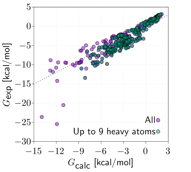
Figure 1: Correlation of experimental, $G_{\rm exp}$, and implicit-solvent, $G_{\rm calc}$, hydration free energies (HFEs) for 355 CHON molecules from the FreeSolv database. The subset of points in green focuses on compounds up to 9 heavy atoms. The dotted line indicates perfect agreement.

We further compare the consistency of calculated implicit-solvent and experimental free-energy datasets by comparing learning curves of ML models. KRR was applied to learn reference free energies obtained by each data set. We use the FreeSolv dataset with up to 9 heavy atoms. For both learning procedures, we rely on the same averaged aSLATM vectors obtained from the conformational ensemble of the simulations. The results for both sets of HFEs are shown in Fig. 2. The implicit-solvation free energies yield better learning performance than the experimental values. Despite a virtually identical slope, the experimental predictions are shifted up by roughly $0.3$ kcal/mol. We point at two possible reasons: ($i$) This shift can be affected by the conformational sampling being identical for both curves, leading to more consistency for the calculated implicit-solvent free energies, as conformational sampling and free energies were obtained from the same set of simulations. ($ii$) However, it could also be caused by the experimental free energies being more heterogeneous. All in all, the results show that implicit-solvent calculations offer a reasonable proxy for the experimental values, which we rely on in the rest of this work.

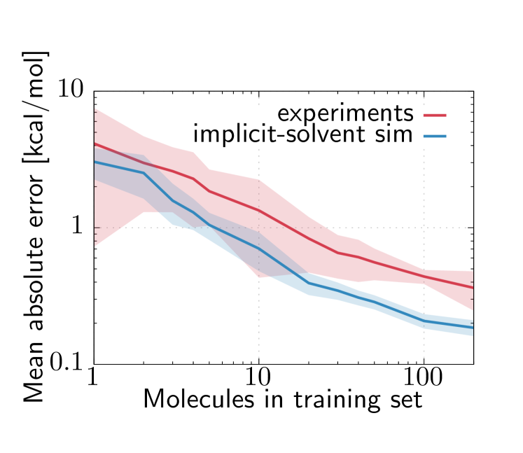
Figure 2: Learning curves for the HFE of the freeSolv dataset using both the experimental and the calculated implicit-solvent free energies. Both curves are averaged over 5 independent simulations.

In the Supporting Information we provide CSV files containing all reference free energies calculated as basis of this work.

III.2 Atomic-decomposition ansatz

We set out to compare the learning performance of HFEs from the molecular representation and the atomic-decomposition ansatz exposed in Section II.3. As a challenging test we specifically focus on learning both types of transferability simultaneously: across databases and compound size. We first picked 663 molecules out of QM9, with 86 and 577 compounds featuring 7 and 8 heavy atoms, respectively. Using this training set we optimized both a global and a local ML model to predict implicit-solvent HFEs. We apply the two ML models to predict the implicit-solvent HFEs of a different set of 351 molecules taken out of the FreeSolv database, which feature a broad range of molecular weights. Fig. 3 displays the mean absolute error of the two ML models as a function of the number of heavy atoms in the predicted (test) compounds. Overall, we find that the global ML model $\hat{K}$ leads to significantly larger errors—up to a factor of 5 in error compared to the atomic kernel for the smallest and largest compounds. The atomic-decomposed ML model, on the other hand, features a slight improvement around 7 and 8 heavy atoms—used for the training set. Furthermore, it displays a remarkably flat behavior (shown on a logarithmic scale), indicating robust transferability across molecular weight. We do observe an increase of the error for molecules toward 15 heavy atoms, likely hinting at a lack of coverage of sufficient chemical environments in the training. The effect may be compounded with significant errors of the implicit-solvent method for large compounds, suggesting a lack of coherence across molecular weight.

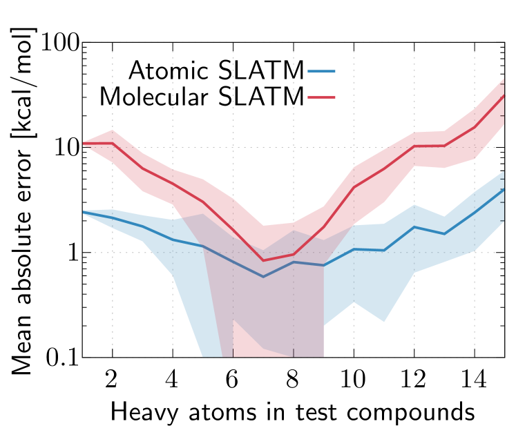
Figure 3: Atomic and Molecular SLATM representations using a KRR model learned on 1000 QM9 compounds with 7 and 8 heavy atoms. Predictions on the FreeSolv database.

The results empirically justify the atomic-decomposition ansatz: the ML model using the aSLATM atom-in-molecule representation reaches better performance across molecular weights, despite the lack of formal justification for Eq. 5. Indeed, the free energy is an ensemble property of the entire system. A decomposition of $G$ into finer components may be considered, for instance via the thermodynamic integration (TI) formula.Kirkwood1935 TI couples the two Hamiltonians of the solute without and with solvent

$$G=\int_{0}^{1}{\rm d}\lambda\left\langle\frac{\partial U}{\partial\lambda}\right\rangle_{\lambda},$$ (10)

where $U$ is the potential energy of the system, $\lambda$ is a coupling parameter between the two Hamiltonians, and $\langle\cdot\rangle_{\lambda}$ denotes an average over the canonical ensemble at coupling parameter $\lambda$. For most explicit-solvent atomistic force fields, the non-bonded interactions of $U$ are pairwise decomposable. In our case, the use of MM-PBSA clouds a simple decomposition, due to the solvation term. However, establishing links between TI and an atom-decomposed ML model may help to shed light on key contributions of the free energy.

The present results indicate that any error due to the decomposition ansatz must be smaller than the accuracy of learning reached from this small dataset. The behavior of the atomic-decomposed ML model as a function of training-set size is probed next.

III.3 Atomic decomposition: Rate of learning

In order to test the performance of our atomic-decomposed ML model, we take as a training set 4000 random molecules sampled from the QM9 database for which we have calculated the HFE using MM/PBSA.

As a baseline model we predict the HFEs using linear regression, with both the 4 elements CHON and the 39 GAFF atom types. Both models were trained on the HFEs of 2000 randomly-selected molecules. We report the mean absolute errors for the held-out 2000 compounds in Tab. 1. The 4-element CHON model has an MAE of $1.80\pm 1.98$ kcal/mol, while the refined 39-atom-type GAFF model yields $1.06\pm 0.02$ kcal/mol. As such, splitting chemical environments in the 39 atom types defined by GAFF almost yield chemical accuracy (1 kcal/mol).

Model name	Parameters	MAE (kcal$/$mol)
CHON elements	4	1.80 $\pm$ 1.98
GAFF atom types	39	1.06 $\pm$ 0.02

Table 1: Mean absolute error for both CHON and GAFF linear regression models. Both models were trained and tested on a 50% hold-out split of 4000 QM9 molecules.

These linear models offer us a way to better assess the performance of the atomic-decomposed ML model. Fig. 4 compares the different regressions in terms of their out-of-sample predictions, displaying the MAE as a function of the training-set size. The atom-decomposed ML model needs 40 and 300 molecules to outperform the CHON and GAFF linear models, respectively. With 2500 molecules in the training set, the atom-decomposed ML model yields an MAE of only 0.7 kcal/mol. It illustrates how offering a richer description consistently improves the performance: from chemical elements (CHON), to a select list of force-field-based atom types (GAFF), to the atom-in-molecule aSLATM representation. The latter can be seen as a continuous generalization of the others, offering a more accurate mapping between local chemical environment and free-energy contribution.

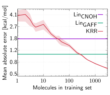
Figure 4: Learning curve of the hydration free energies for 4000 randomly chosen molecules of the QM9 database. The two lines show the prediction error for the CHON and GAFF linear models. KRR is the atomic-decomposed ML model.

III.4 Database bias

If learning HFEs across a subset of QM9 requires $\sim 10^{2}$ training compounds, how transferable is this result to other databases? We set the stage for this question by comparing atom-decomposed learning in three different databases, which differently try to span chemical space: QM9, eMolecules, and FreeSolv. We will more directly address the question further down in Sec. III.5.

Figure 5 shows independent learning curves for the three databases. While QM9 and eMolecules show similar learning performance—the latter being slightly more performant—we observe surprisingly different behavior for FreeSolv: the learning curve reaches chemical accuracy after less than 10 compounds, and only 0.3 kcal/mol after 200 training molecules. The three ML models featuring identical architectures and representations, the results suggest a significant bias in the nature of the subsets of chemical space they span.

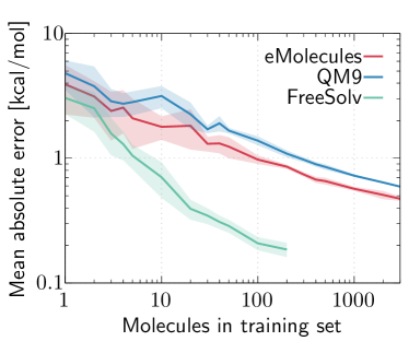
Figure 5: Learning curves for the HFE ML models for the three databases QM9, eMolecules and FreeSolv. All curves are averaged over 5 independent runs.

To probe the difference in the spanned chemistries of the three databases, we performed dimensionality reduction. We used the UMAP algorithm.mcinnes2018umap UMAP builds a fuzzy topological representation in the original high-dimensional space, and identifies a low-dimensional embedding by means of a cross-entropy measure. The UMAP parameters consisted of the number of neighbors (15), the minimum distance (0.1), the dimensionality of the embedding (1 or 2), and the metric (Euclidean).

To compare the three databases we need to project them onto the same reduced subspace. A one-dimensional (1D) projection was first trained from the atomic SLATM representation on QM9, as we assumed QM9 to cover chemical space more broadly than the other two, since it represents a subset of the GDB. After training we map all three databases onto this 1D projection, subsequently called $\varphi_{1}$. Fig. 6a shows the probability distribution, $p(\varphi_{1})$, as a measure of coverage in that subspace. The results are striking: While QM9 shows a remarkably flat distribution across the range of $\varphi_{1}$, eMolecules displays larger fluctuations, while FreeSolv yields high peaks, indicating significant localization within the subspace. This localization translates into significant bias in the chemical space spanned by the database—most atomic environments cluster at few points within the $\varphi_{1}$ subspace. This behavior explains the exceptional learning behavior shown in Fig. 5. The intermediate regime of eMolecules (between broad and spiked) indicates slight but noticeable localizations in chemical space, translating in learning performance that is slightly more favorable than QM9. As such the commercially available database shows less diversity than the algorithmically generated database.

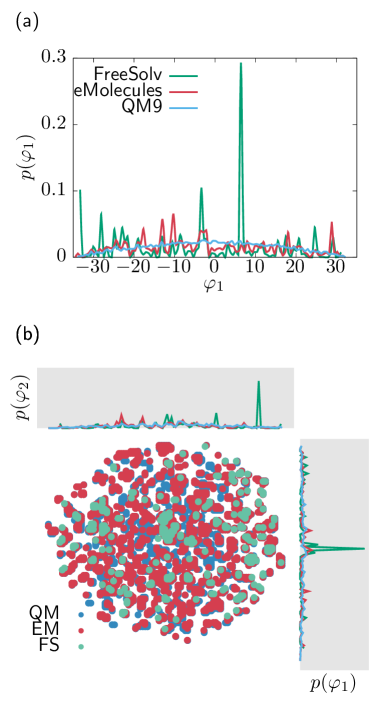
Figure 6: (a) Probability distribution, $p(\varphi_{1})$, of the 1D UMAP projection of the three databases. (b) Probability distribution, $p(\varphi_{1},\varphi_{2})$, and 1-dimensional cuts of the 2D UMAP projection of the three databases QM9 (QM), eMolecules (EM), and FreeSolv (FS).

The same trend applies when mapping to a 2-dimensional (2D) mapping of the chemical space spanned by these databases. A similar training procedure is applied as for the 1D case. Fig. 6b shows the 2D probability distribution, $p(\varphi_{1},\varphi_{2})$, as well as 1D cuts thereof. The sharp peaks of FreeSolv subsist in both dimensions. The 2D space more explicitly illustrates the presence of “islands” in chemical space—most strongly pronounced for FreeSolv—but we also find significant differences between QM9 and eMolecules.

III.5 Cross-Learning

To further probe the overlap between subsets of chemical space spanned by the three datasets, we performed cross-learning experiments, in which we train on one dataset and predict on another. For FreeSolv all 259 molecules were used for the training and test sets, while for QM9 and eMolecules we considered all 4000 molecules for training, and up to 3000 randomly-selected compounds for testing. Fig. 7 and Tab. 2 report the cross-learning results for our ML models, which we analyze in the following.

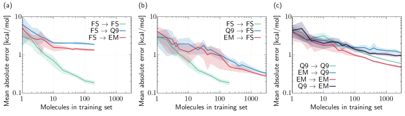
Figure 7: Learning curves for the cross-learning experiments: training on one dataset and prediction on another. FS, EM, and QM stand for FreeSolv, eMolecules, and QM9, respectively. The legends indicate the type of cross-learning: $X\to Y$ means training on $X$ and prediction on $Y$.

Training	Prediction
	QM9	eMolecules	FreeSolv
QM9	$0.65\pm 0.02$	$1.00\pm 0.03$	$0.36\pm 0.02$
eMolecules	$1.26\pm 0.05$	$0.61\pm 0.01$	$0.35\pm 0.01$
FreeSolv	$2.04\pm 0.06$	$1.26\pm 0.05$	$0.24\pm 0.02$

Table 2: Cross-learning machine learning models of the three databases considered in this study. All energies given in kcal/mol.

Fig. 7a reports cross-learning trained on the FreeSolv database. The FreeSolv $\to$ FreeSolv is identical to what was shown in Fig. 5, and cross-learning to the other databases shows a significant deterioration of the accuracy: QM9 and eMolecules saturate to roughly 1.9 and 1.3 kcal/mol. We recall the results from Fig. 4: the CHON and GAFF linear models reach an accuracy of 1.80 and 1.06 kcal/mol. As such the FreeSolv cross-learning on QM9 is worse than a 4-parameter linear regression. Beyond the MAEs at highest training size, what is striking is the apparent plateau behavior after the first decade of training points: Learning improves negligibly from 10 to $10^{2}$ data points. This aspect speaks for the lack of breadth of chemical space—the dataset features few, overrepresented chemical environments. Furthermore, the small but noticeable offset between eMolecules and QM9 suggests more difficulties in learning the latter, which further hints at its broader diversity of chemical environments.

Panel b of Fig. 7 demonstrates the opposite effect: to what extent the three databases can predict FreeSolv. All three databases eventually lead to similar accuracy, albeit with different learning rates: FreeSolv is more efficient at learning itself than the others, while QM9 and eMolecules show significant offsets. This is another hint at the broader diversity of compounds from eMolecules and, to a larger extent, QM9.

Finally, Fig. 7c focuses on the comparison between eMolecules and QM9. All curves roughly start at the same offset at low training data. Both self-learning curves (QM9 $\to$ QM9 and eMolecules $\to$ eMolecules) reach the lowest MAE, thanks to a slightly more favorable rate of learning. When it comes to cross-learning, QM9 shows a slight advantage at learning eMolecules than vice versa. Based on the dimensionality reduction (Fig. 6), we argue that this arises from the broader diversity of chemical environments present in QM9.

IV Conclusions

In the present work we study the machine learning (ML) of hydration free energies (HFEs) across a subset of small organic molecules—those made of chemical elements C, H, O, and N. To probe the effects of database biases on the learning of thermodynamic properties, we generated reference HFEs using implicit-solvent computer simulations at an atomistic resolution. We find that an atomic-decomposition ansatz, in which we assume a linear decomposition of the HFE in atomic contributions, offers remarkable transferability, compared to the more straightforward learning of the molecular property. As baseline we compare two linear models based on atom types, as often used in force fields. A 39-parameter model based on the GAFF atom types yields 1.06 kcal/mol. Training a better performing atom-decomposed ML model requires a couple hundred molecules in the training set. The atom-in-molecule environment encoded in the aSLATM representation offers de facto a generalization of the concept of force-field atom types.

ML models trained on different databases show significantly different performance. Using dimensionality reduction, we find that FreeSolv and eMolecules, two databases of commercially available compounds, show strong localizations in the chemical space spanned. We can very efficiently train an ML model out of the FreeSolv database, but it fails to generalize to the other databases. Furthermore, cross-learning across databases shows that training a model on FreeSolv and deploying it on QM9 is worse than a 4-parameter linear model, and shows a severe plateau behavior, highlighting the lack of chemical diversity. The combination of cross-learning and dimensionality reduction shows that supervised learning can help empirically establish which database probes a broader chemical space. It also shows that deploying an ML model on independent databases can help probe its generalization.

V Supplementary Material

CSV data files for subsets of the FreeSolv,mobley2014freesolv eMolecules,emolecules and QM9ramakrishnan2014quantum databases containing SMILES strings and associated hydration free energies, as calculated from atomistic simulations with implicit solvent. The data file for FreeSolv additionally contains reference experimental free energies.mobley2014freesolv

VI Acknowledgements

We thank Bernadette Mohr and Roberto Menichetti for critical reading of the manuscript. We also thank Denis Andrienko, Kiran H. Kanekal, and Christoph Scherer for insightful discussions. This work was partially supported by the Emmy Noether program of the Deutsche Forchungsgemeinschaft (DFG). TB acknowledges the Institute for Pure and Applied Mathematics (IPAM), which is supported by the National Science Foundation (Grant No. DMS-1440415).

VII Data availability

The data that supports the findings of this study are available within the article and its supplementary material.

References

- [1] Jörg Behler. Perspective: Machine learning potentials for atomistic simulations. The Journal of chemical physics, 145(17):170901, 2016.
- [2] Raghunathan Ramakrishnan and O Anatole von Lilienfeld. Machine learning, quantum chemistry, and chemical space. Reviews in Computational Chemistry, pages 225–256, 2017.
- [3] Benjamin Sanchez-Lengeling and Alán Aspuru-Guzik. Inverse molecular design using machine learning: Generative models for matter engineering. Science, 361(6400):360–365, 2018.
- [4] O Anatole Von Lilienfeld. Quantum machine learning in chemical compound space. Angewandte Chemie International Edition, 57(16):4164–4169, 2018.
- [5] Albert P Bartók, Risi Kondor, and Gábor Csányi. On representing chemical environments. Physical Review B, 87(18):184115, 2013.
- [6] Kristof T Schütt, Farhad Arbabzadah, Stefan Chmiela, Klaus R Müller, and Alexandre Tkatchenko. Quantum-chemical insights from deep tensor neural networks. Nature communications, 8(1):1–8, 2017.
- [7] Haoyan Huo and Matthias Rupp. Unified representation for machine learning of molecules and crystals. arXiv preprint arXiv:1704.06439, 13754, 2017.
- [8] Stefan Chmiela, Alexandre Tkatchenko, Huziel E Sauceda, Igor Poltavsky, Kristof T Schütt, and Klaus-Robert Müller. Machine learning of accurate energy-conserving molecular force fields. Science advances, 3(5):e1603015, 2017.
- [9] Aldo Glielmo, Peter Sollich, and Alessandro De Vita. Accurate interatomic force fields via machine learning with covariant kernels. Physical Review B, 95(21):214302, 2017.
- [10] Andrea Grisafi, David M Wilkins, Gábor Csányi, and Michele Ceriotti. Symmetry-adapted machine learning for tensorial properties of atomistic systems. Physical review letters, 120(3):036002, 2018.
- [11] Tristan Bereau, Robert A DiStasio Jr, Alexandre Tkatchenko, and O Anatole Von Lilienfeld. Non-covalent interactions across organic and biological subsets of chemical space: Physics-based potentials parametrized from machine learning. The Journal of chemical physics, 148(24):241706, 2018.
- [12] Nathaniel Thomas, Tess Smidt, Steven Kearnes, Lusann Yang, Li Li, Kai Kohlhoff, and Patrick Riley. Tensor field networks: Rotation-and translation-equivariant neural networks for 3d point clouds. arXiv preprint arXiv:1802.08219, 2018.
- [13] Matthias Rupp, Alexandre Tkatchenko, Klaus-Robert Müller, and O Anatole Von Lilienfeld. Fast and accurate modeling of molecular atomization energies with machine learning. Physical review letters, 108(5):058301, 2012.
- [14] Katja Hansen, Grégoire Montavon, Franziska Biegler, Siamac Fazli, Matthias Rupp, Matthias Scheffler, O Anatole Von Lilienfeld, Alexandre Tkatchenko, and Klaus-Robert Müller. Assessment and validation of machine learning methods for predicting molecular atomization energies. Journal of Chemical Theory and Computation, 9(8):3404–3419, 2013.
- [15] Tristan Bereau, Denis Andrienko, and O Anatole von Lilienfeld. Transferable atomic multipole machine learning models for small organic molecules. Journal of chemical theory and computation, 11(7):3225–3233, 2015.
- [16] Michael Gastegger, Jörg Behler, and Philipp Marquetand. Machine learning molecular dynamics for the simulation of infrared spectra. Chemical science, 8(10):6924–6935, 2017.
- [17] Andrea Grisafi, Alberto Fabrizio, Benjamin Meyer, David M Wilkins, Clemence Corminboeuf, and Michele Ceriotti. Transferable machine-learning model of the electron density. ACS Central Science, 5(1):57–64, 2018.
- [18] KT Schütt, Michael Gastegger, Alexandre Tkatchenko, K-R Müller, and Reinhard J Maurer. Unifying machine learning and quantum chemistry with a deep neural network for molecular wavefunctions. Nature communications, 10(1):1–10, 2019.
- [19] Tristan Bereau, Denis Andrienko, and Kurt Kremer. Research update: Computational materials discovery in soft matter. APL Materials, 4(5):053101, 2016.
- [20] Andrew L Ferguson. Machine learning and data science in soft materials engineering. Journal of Physics: Condensed Matter, 30(4):043002, 2017.
- [21] Tristan Bereau. Data-driven methods in multiscale modeling of soft matter. In Handbook of Materials Modeling, pages 1–12. Springer International Publishing, 2018.
- [22] Nicholas E Jackson, Michael A Webb, and Juan J de Pablo. Recent advances in machine learning towards multiscale soft materials design. Current Opinion in Chemical Engineering, 23:106–114, 2019.
- [23] ST John and Gábor Csányi. Many-body coarse-grained interactions using gaussian approximation potentials. The Journal of Physical Chemistry B, 121(48):10934–10949, 2017.
- [24] Jiang Wang, Simon Olsson, Christoph Wehmeyer, Adrià Pérez, Nicholas E Charron, Gianni De Fabritiis, Frank Noé, and Cecilia Clementi. Machine learning of coarse-grained molecular dynamics force fields. ACS central science, 5(5):755–767, 2019.
- [25] Henry Chan, Mathew J Cherukara, Badri Narayanan, Troy D Loeffler, Chris Benmore, Stephen K Gray, and Subramanian KRS Sankaranarayanan. Machine learning coarse grained models for water. Nature communications, 10(1):1–14, 2019.
- [26] Alireza Moradzadeh and Narayana R Aluru. Transfer-learning-based coarse-graining method for simple fluids: Toward deep inverse liquid-state theory. The journal of physical chemistry letters, 10(6):1242–1250, 2019.
- [27] Mohammad M Sultan and Vijay S Pande. Automated design of collective variables using supervised machine learning. The Journal of chemical physics, 149(9):094106, 2018.
- [28] Christoph Wehmeyer and Frank Noé. Time-lagged autoencoders: Deep learning of slow collective variables for molecular kinetics. The Journal of chemical physics, 148(24):241703, 2018.
- [29] Yasemin Bozkurt Varolgunes, Tristan Bereau, and Joseph F Rudzinski. Interpretable embeddings from molecular simulations using gaussian mixture variational autoencoders. Machine Learning: Science and Technology, 2020.
- [30] Ernest Y Lee, Benjamin M Fulan, Gerard CL Wong, and Andrew L Ferguson. Mapping membrane activity in undiscovered peptide sequence space using machine learning. Proceedings of the National Academy of Sciences, 113(48):13588–13593, 2016.
- [31] Christian Hoffmann, Roberto Menichetti, Kiran H Kanekal, and Tristan Bereau. Controlled exploration of chemical space by machine learning of coarse-grained representations. Physical Review E, 100(3):033302, 2019.
- [32] Anton J Hopfinger and Robert D Battershell. Application of scap to drug design. 1. prediction of octanol-water partition coefficients using solvent-dependent conformational analyses. Journal of medicinal chemistry, 19(5):569–573, 1976.
- [33] Garland R Marshall. Computer-aided drug design. Annual review of pharmacology and toxicology, 27(1):193–213, 1987.
- [34] Andrew R Leach, Brian K Shoichet, and Catherine E Peishoff. Prediction of protein-ligand interactions. docking and scoring: Successes and gaps. Journal of medicinal chemistry, 49(20):5851–5855, 2006.
- [35] Hugo Kubinyi. 3D QSAR in drug design: volume 1: theory methods and applications, volume 1. Springer Science & Business Media, 1993.
- [36] Fahimeh Ghasemi, Alireza Mehridehnavi, Alfonso Perez-Garrido, and Horacio Perez-Sanchez. Neural network and deep-learning algorithms used in qsar studies: merits and drawbacks. Drug Discov. Today, 23(10):1784–1790, 2018.
- [37] Han Altae-Tran, Bharath Ramsundar, Aneesh S Pappu, and Vijay Pande. Low data drug discovery with one-shot learning. ACS central science, 3(4):283–293, 2017.
- [38] Arkadii Lin, Dragos Horvath, Valentina Afonina, Gilles Marcou, Jean-Louis Reymond, and Alexandre Varnek. Mapping of the available chemical space versus the chemical universe of lead-like compounds. ChemMedChem, 13(6):540–554, January 2018.
- [39] Marta Glavatskikh, Jules Leguy, Gilles Hunault, Thomas Cauchy, and Benoit Da Mota. Dataset’s chemical diversity limits the generalizability of machine learning predictions. Journal of Cheminformatics, 11(1):69, 2019.
- [40] Christopher M Dobson. Chemical space and biology. Nature, 432(7019):824, 2004.
- [41] Jean-Louis Reymond. The chemical space project. Accounts of chemical research, 48(3):722–730, 2015.
- [42] Roberto Menichetti, Kiran H Kanekal, and Tristan Bereau. Drug–membrane permeability across chemical space. ACS central science, 5(2):290–298, 2019.
- [43] Lars Ruddigkeit, Ruud Van Deursen, Lorenz C Blum, and Jean-Louis Reymond. Enumeration of 166 billion organic small molecules in the chemical universe database gdb-17. Journal of chemical information and modeling, 52(11):2864–2875, 2012.
- [44] Roman Zubatyuk, Justin S Smith, Jerzy Leszczynski, and Olexandr Isayev. Accurate and transferable multitask prediction of chemical properties with an atoms-in-molecules neural network. Science advances, 5(8):eaav6490, 2019.
- [45] Samuel T Hutchinson and Rika Kobayashi. Solvent-specific featurization for predicting free energies of solvation through machine learning. J. Chem. Inf. Model., 59(4):1338–1346, 2019.
- [46] Hyuntae Lim and YounJoon Jung. Delfos: deep learning model for prediction of solvation free energies in generic organic solvents. Chemical Science, 10(36):8306–8315, 2019.
- [47] Raghunathan Ramakrishnan, Pavlo O Dral, Matthias Rupp, and O Anatole Von Lilienfeld. Quantum chemistry structures and properties of 134 kilo molecules. Scientific data, 1:140022, 2014.
- [48] eMolecules. https://www.emolecules.com.
- [49] David L Mobley and J Peter Guthrie. Freesolv: a database of experimental and calculated hydration free energies, with input files. Journal of computer-aided molecular design, 28(7):711–720, 2014.
- [50] Devleena Shivakumar, Joshua Williams, Yujie Wu, Wolfgang Damm, John Shelley, and Woody Sherman. Prediction of absolute solvation free energies using molecular dynamics free energy perturbation and the opls force field. Journal of chemical theory and computation, 6(5):1509–1519, 2010.
- [51] Zied Gaieb, Shuai Liu, Symon Gathiaka, Michael Chiu, Huanwang Yang, Chenghua Shao, Victoria A Feher, W Patrick Walters, Bernd Kuhn, Markus G Rudolph, et al. D3r grand challenge 2: blind prediction of protein–ligand poses, affinity rankings, and relative binding free energies. Journal of computer-aided molecular design, 32(1):1–20, 2018.
- [52] Samuel Genheden and Ulf Ryde. The mm/pbsa and mm/gbsa methods to estimate ligand-binding affinities. Expert opinion on drug discovery, 10(5):449–461, 2015.
- [53] Anthony Nicholls, David L Mobley, J Peter Guthrie, John D Chodera, Christopher I Bayly, Matthew D Cooper, and Vijay S Pande. Predicting small-molecule solvation free energies: an informal blind test for computational chemistry. Journal of medicinal chemistry, 51(4):769–779, 2008.
- [54] Junmei Wang, Wei Wang, Peter A Kollman, and David A Case. Antechamber: an accessory software package for molecular mechanical calculations. J. Am. Chem. Soc, 222:U403, 2001.
- [55] Bing Huang and O Anatole von Lilienfeld. The “dna” of chemistry: Scalable quantum machine learning with “amons”. arXiv preprint arXiv:1707.04146, 2017.
- [56] Bing Huang, Nadine O. Symonds, and O. Anatole von Lilienfeld. Quantum machine learning in chemistry and materials. In Handbook of Materials Modeling, pages 1–27. Springer International Publishing, 2018.
- [57] Michele Ceriotti, Michael J. Willatt, and Gábor Csányi. Machine learning of atomic-scale properties based on physical principles. In Handbook of Materials Modeling, pages 1–27. Springer International Publishing, 2018.
- [58] Christoph Scherer, Rene Scheid, Denis Andrienko, and Tristan Bereau. Kernel-based machine learning for efficient simulations of molecular liquids. Journal of Chemical Theory and Computation, 16(5):3194–3204, April 2020.
- [59] Mark James Abraham, Teemu Murtola, Roland Schulz, Szilárd Páll, Jeremy C. Smith, Berk Hess, and Erik Lindahl. GROMACS: High performance molecular simulations through multi-level parallelism from laptops to supercomputers. SoftwareX, 1-2:19–25, September 2015.
- [60] RDKit: open-source cheminformatics. http://www.rdkit.org.
- [61] Alan W Sousa Da Silva and Wim F Vranken. Acpype-antechamber python parser interface. BMC research notes, 5(1):367, 2012.
- [62] Rashmi Kumari, Rajendra Kumar, Open Source Drug Discovery Consortium, and Andrew Lynn. g_mmpbsa—a GROMACS tool for high-throughput MM-PBSA calculations. Journal of Chemical Information and Modeling, 54(7):1951–1962, 2014.
- [63] Nathan A. Baker, David Sept, Simpson Joseph, Michael J. Holst, and J. Andrew McCammon. Electrostatics of nanosystems: Application to microtubules and the ribosome. Proc. Natl. Acad. Sci., 98(18):10037–10041, 2001.
- [64] John G. Kirkwood. Statistical mechanics of fluid mixtures. The Journal of Chemical Physics, 3(5):300–313, May 1935.
- [65] Leland McInnes, John Healy, and James Melville. Umap: Uniform manifold approximation and projection for dimension reduction. arXiv preprint arXiv:1802.03426, 2018.