Nitsche’s method for Kirchhoff plates

Abstract

We introduce a Nitsche’s method for the numerical approximation of the Kirchhoff–Love plate equation under general Robin-type boundary conditions. We analyze the method by presenting a priori and a posteriori error estimates in mesh-dependent norms. Several numerical examples are given to validate the approach and demonstrate its properties.

65N30

1 Introduction

Implementation of $H^{2}$-conforming finite element methods can be a challenge due to the $C^{1}$-continuity requirement of the finite element basis [7]. In fact, it is a common motivation for developing discontinuous Galerkin techniques [5] where it is sufficient to guarantee the conformity in a weak sense only, other nonconforming methods using special finite elements [2, 3], or mixed methods [1] where the fourth-order problem is split into a system of lower order problems. At the same time, however, finite element codes including classical $H^{2}$-conforming elements—such as, e.g., the Argyris triangle and the rectangular Bogner–Fox–Schmit element [25]—abound and many are free and readily available [8, 22, 14, 23] to be used in the discretization of fourth-order differential operators. Thus, the main challenge remaining for the end user is the proper implementation of external loads and boundary conditions.

In [21], Nitsche introduced a consistent penalty-type method for imposing Dirichlet boundary conditions in the second-order Poisson problem. Nitsche’s method was extended to other boundary conditions (in particular, inhomogeneous Robin) in Juntunen–Stenberg [16] by unifying the implementation and analysis via a parameter-dependent boundary value problem; an improved a priori analysis was presented in Lüthen–Juntunen–Stenberg [19]. Different boundary conditions (Dirichlet, Neumann, Robin) were obtained by changing the value of a single nonnegative parameter. The resulting method performed similarly well in all cases, i.e. altering the parameter value did not deteoriate the conditioning of the resulting linear system or lead to an overrefinement as in traditional methods.

In this study we explore the above ideas [21, 16, 19] in the context of fourth-order $H^{2}$-conforming problems. In particular, we seek to unify the implementation and the analysis of different boundary conditions for the Kirchhoff–Love plate equation [17, 18] by presenting a Nitsche’s method which incorporates the boundary conditions in the discrete formulation as consistent penalty terms. We consider elastic Robin-type boundary conditions for the deflection and the rotation including applied external forces and moments. The classical boundary conditions for the Kirchhoff plates (clamped, simply supported and free) are recovered as special cases. Moreover, we allow general matching conditions at the corners of the domain so that ball supports, point forces and springs [10, 4, 24] are all covered by the same formalism.

Figure 1: Definition sketch of the plate with different boundary conditions and elastic supports: springs at $c_{1}$ and $c_{4}$, a ball support at $c_{2}$, applied point forces at $c_{4}$ and $c_{5}$, an applied shear force on $\Gamma_{1}$, a spring support on $\Gamma_{2}$ and $\Gamma_{3}$, an applied torque on $\Gamma_{3}$, a torsion spring support on $\Gamma_{4}$.

The Nitsche method is not only practical to implement but has also other advantages. For a very stiff support, i.e. with almost clamped conditions, the traditional method leads to two potential problems: 1) the corresponding stiffness matrix becomes ill-conditioned and 2) the standard a posteriori estimators lead to overrefinement. As for the Poisson problem, these phenomena can be avoided using the Nitsche method presented in this work. Moreover, if one is using plate elements in which second derivatives are included as degrees-of-freedom, e.g., the Argyris triangle and the Bogner–Fox–Schmit element, and if the boundary conditions are enforced by eliminating degrees-of-freedom, one must verify separately that the second-order derivatives are zero along the boundary of the domain. In practice, e.g., in case of non-right angles, this introduces additional linear constraints for the solution to satisfy. Nitsche’s method circumvents this issue by enforcing the boundary conditions weakly.

The rest of the paper is organized as follows. In Section 2, we introduce the Kirchhoff plate bending model and its boundary conditions. In Section 3, we derive the Nitsche method by augmenting the model’s weak formulation with consistent penalty-type terms. In Section 4, we prove the stability of the resulting discrete formulation and present the ensuing a priori error estimate. In Section 5, we present the residual a posteriori error estimators and prove an error estimate via a saturation assumption. Finally in Section 6, we demonstrate the approach by performing computational experiments.

2 The Kirchhoff plate model

We start by recalling the Kirchhoff plate model with general boundary conditions, cf. [10, 20, 9]. Let $\Omega\subset\mathbb{R}^{2}$ be a polygonal domain, with corners $c_{i}$, and the boundary $\partial\Omega=\cup_{i=1}^{m}\Gamma_{i}$, $i=1,\dots,m$, where each $\Gamma_{i}$ is a line segment, see Figure 1. Given the deflection $u:\Omega\to\mathbb{R}$ of the midsurface of the plate, the curvature $\boldsymbol{K}$ is defined through

(2.1) $$\boldsymbol{K}(u)=-\boldsymbol{\varepsilon}(\nabla u),$$

where the infinitesimal strain $\boldsymbol{\varepsilon}$ is given by

(2.2) $$\boldsymbol{\varepsilon}(\boldsymbol{v})=\frac{1}{2}\left\lparen\nabla\boldsymbol{v}+\nabla\boldsymbol{v}^{T}\right\rparen,\quad(\nabla\boldsymbol{v})_{ij}=\frac{\partial v_{i}}{\partial x_{j}},\quad i,j=1,2.$$

The moment tensor $\boldsymbol{M}$ is given by the constitutive relation

(2.3) $$\qquad\boldsymbol{M}(u)=\frac{Ed^{3}}{12(1+\nu)}\left\lparen\boldsymbol{K}(u)+\frac{\nu}{1-\nu}(\text{tr}\,\boldsymbol{K}(u))\boldsymbol{I}\right\rparen,$$

where $d$ denotes the plate thickness and $\boldsymbol{I}$ is the identity tensor. Above, $E$ and $\nu$ are the Young’s modulus and the Poisson ratio, respectively.

The shear force $\boldsymbol{Q}$ is related to the moment tensor through the moment equilibrium equation

(2.4) $$\boldsymbol{\mathrm{div}\,}\boldsymbol{M}(u)=\boldsymbol{Q}(u),$$

where $\boldsymbol{\mathrm{div}\,}$ is the vector-valued divergence operator. The transverse shear equilibrium reads as follows

(2.5) $$-\mathrm{div}\,\boldsymbol{Q}(u)=f$$

where $f$ is an external transverse loading. Combining the above expressions yields the Kirchhoff–Love plate equation

(2.6) $$D\Delta^{2}u=f,$$

where $D$, the plate rigidity, is defined as

(2.7) $$D=\frac{Ed^{3}}{12(1-\nu^{2})}.$$

We consider quite general boundary conditions. A vertical force $g^{v}_{i}$ and a normal moment $g^{r}_{i}$ act on each segment $\Gamma_{i}$ of the boundary and the support is elastic with respect to both the deflection and the rotation, with the spring constants $1/\varepsilon^{v}_{i}$ and $1/\varepsilon^{r}_{i}$, respectively. At the corner $c_{i}$, also connected to a spring with constant $1/\varepsilon^{c}_{i}$, acts a point force $g^{c}_{i}$.

The energy of the system can be written as

(2.8) $$I(v) =\frac{1}{2}\int_{\Omega}\boldsymbol{M}(v):\boldsymbol{K}(v)\,\mathrm{d}x$$

$$\phantom{=}~{}+\sum_{i=1}^{m}\bigg{\{}\frac{1}{2\varepsilon^{v}_{i}}\int_{\Gamma_{i}}v^{2}\,\mathrm{d}s+\frac{1}{2\varepsilon^{r}_{i}}\int_{\Gamma_{i}}\Big{(}\frac{\partial v}{\partial\boldsymbol{n}}\Big{)}^{2}\mathrm{d}s+\frac{1}{2\varepsilon^{c}_{i}}v(c_{i})^{2}$$

$$\qquad\qquad~{}~{}-\int_{\Gamma_{i}}g^{v}_{i}v\,\mathrm{d}s+\int_{\Gamma_{i}}g^{r}_{i}\frac{\partial v}{\partial\boldsymbol{n}}\,\mathrm{d}s-\sum_{i=1}^{m}g^{c}_{i}v(c_{i})\bigg{\}}-\int_{\Omega}fv\,\mathrm{d}x,$$

from where follows the variational formulation: find $u\in H^{2}(\Omega)$ such that

(2.9) $$\int_{\Omega}\boldsymbol{M}(u):\boldsymbol{K}(v)\,\mathrm{d}x+\sum_{i=1}^{m}\bigg{\{}\frac{1}{\varepsilon^{v}_{i}}\int_{\Gamma_{i}}uv\,\mathrm{d}s+\frac{1}{\varepsilon^{r}_{i}}\int_{\Gamma_{i}}\frac{\partial u}{\partial\boldsymbol{n}}\frac{\partial v}{\partial\boldsymbol{n}}\mathrm{d}s+\frac{1}{\varepsilon^{c}_{i}}u(c_{i})v(c_{i})\bigg{\}}$$

$$=\int_{\Omega}fv\,\mathrm{d}x+\sum_{i=1}^{m}\bigg{\{}\int_{\Gamma_{i}}g^{v}_{i}v\,\mathrm{d}s-\int_{\Gamma_{i}}g^{r}_{i}\frac{\partial v}{\partial\boldsymbol{n}}\,\mathrm{d}s+\sum_{i=1}^{m}g^{c}_{i}v(c_{i})\bigg{\}}\quad\forall v\in H^{2}(\Omega).$$

The corresponding boundary value problem is posed using the normal shear force, and the normal and twisting moments

(2.10) $$Q_{n}(w) =\boldsymbol{Q}(w)\cdot\boldsymbol{n},$$

$$M_{nn}(w) =\boldsymbol{n}\cdot\boldsymbol{M}(w)\boldsymbol{n},$$

$$M_{ns}(w) =M_{sn}(w)=\boldsymbol{s}\cdot\boldsymbol{M}(w)\boldsymbol{n}.$$

Above $\boldsymbol{n}$ denotes the outward unit normal on $\partial\Omega$ and $\boldsymbol{s}=(n_{1},-n_{2})$ is the respective unit tangent vector. Moreover, we define the Kirchhoff shear force as

(2.11) $$V_{n}(w)=Q_{n}(w)+\frac{\partial M_{ns}(w)}{\partial s},$$

and the jump in the twisting moment

(2.12) $$\llbracket M_{ns}(u)\rrbracket|_{c_{i}}=\lim_{\epsilon\rightarrow 0+}\Big{(}M_{ns}(u)|_{c_{i}+\epsilon(c_{i+1}-c_{i})}-M_{ns}(u)|_{c_{i}+\epsilon(c_{i-1}-c_{i})}\Big{)},$$

$i=1,\dots,m,$ with $c_{m+1}=c_{1}$. After repeated integrations by parts, one then obtains

(2.13) $$\int_{\Omega}D\Delta^{2}uv\,\mathrm{d}x= \int_{\Omega}\boldsymbol{M}(u):\boldsymbol{K}(v)\,\mathrm{d}x$$

$$+\sum_{i=1}^{m}\bigg{\{}\int_{\Gamma_{i}}M_{nn}(u)\frac{\partial v}{\partial\boldsymbol{n}}\,\mathrm{d}s$$

$$\qquad~{}~{}~{}~{}-\int_{\Gamma_{i}}V_{n}(u)v\,\mathrm{d}s-\llbracket M_{ns}(u)\rrbracket|_{c_{i}}v(c_{i})\bigg{\}}.$$

Substituting (2.13) into the weak form (2.9) leads to the differential equation (2.6) and the boundary conditions on $\Gamma_{i}$

(2.14) $$V_{n}(u)+\frac{1}{\varepsilon^{v}_{i}}u=g^{v}_{i},\quad M_{nn}(u)-\frac{1}{\varepsilon^{r}_{i}}\frac{\partial u}{\partial\boldsymbol{n}}=g^{r}_{i},\ i=1,\dots,m,$$

and the corner conditions

(2.15) $$\llbracket M_{ns}(u)\rrbracket|_{c_{i}}+\frac{1}{\varepsilon^{c}_{i}}u(c_{i})=g^{c}_{i},\quad i=1,\ldots,m,$$

with the letters $v,r,c$ indicating vertical, rotational and corner, respectively. The boundary value problem is now formed by the equations (2.6), (2.14) and (2.15).

Remark 1.

The boundary and corner conditions (2.14) and (2.15) include

• clamped at edge $\Gamma_{i}$ when $\varepsilon^{v}_{i},\varepsilon^{r}_{i},\varepsilon^{c}_{i},\varepsilon^{c}_{i+1}\rightarrow 0$,

• simply supported at edge $\Gamma_{i}$ when $\varepsilon^{v}_{i},\varepsilon^{c}_{i},\varepsilon^{c}_{i+1}\rightarrow 0$, $\varepsilon^{r}_{i}\rightarrow\infty$, $g^{r}_{i}=0$,

• free at edge $\Gamma_{i}$ when $\varepsilon^{v}_{i},\varepsilon^{r}_{i},\varepsilon^{c}_{i},\varepsilon^{c}_{i+1}\rightarrow\infty$ and $g^{v}_{i}=g^{r}_{i}=g^{c}_{i}=g_{i+1}^{c}=0$,

and various other combinations of prescribed forces and moments on the boundary and at the corners of the domain.

3 The finite element method

The domain $\Omega$ is split into non-overlapping regular elements $K\in\mathcal{C}_{h}$. As usual, the mesh parameter is $h=\max_{K\in\mathcal{C}_{h}}h_{K}$. The set of the interior edges of the mesh is denoted by $\mathcal{E}_{h}$ and the set of the boundary edges by $\mathcal{G}_{h}$. By $h_{E}$ we denote the length of the edge $E\in\mathcal{E}_{h}\cup\mathcal{G}_{h}$ and by $h_{i}=\max_{K\in\mathcal{C}_{h},c_{i}\in K}h_{K}$ the local mesh length around the corner $c_{i}$.

At times, we write in the estimates $a\lesssim b$ (or $a\gtrsim b$) when $a\leq Cb$ (or $a\geq Cb$), for some positive constant $C$, independent of the mesh parameter $h$ and the parameters $\varepsilon^{v}_{i},\varepsilon^{r}_{i},\varepsilon^{c}_{i}$. Moreover, we use the standard notation $(\cdot,\cdot)_{R}$ for the $L^{2}(R)$-inner product and write $(\cdot,\cdot)$ for the $L^{2}(\Omega)$-inner product.

The (conforming) finite element space is defined as

(3.1) $$V_{h}=\{v\in H^{2}(\Omega):v|_{K}\in V_{K}\ \forall K\in\mathcal{C}_{h}\}$$

with the polynomial $V_{K}$ space satisfying

(3.2) $$P_{p}(K)\subset V_{K}\subset P_{l}(K),$$

for some $p$ and $l$; $P_{l}(K)$ is the complete space of polynomials of degree $l$ in $K$. Examples of such spaces include (cf. [6]), the Argyris triangle with $p=l=5$, the Bell triangle with $p=3$ and $l=5$ and the Bogner–Fox–Schmit rectangular element with $p=3$ and $l=6$. The Hsieh–Clough–Tocher element is another option, but will lead to an additional term in the a posteriori estimator and hence is not included in the analysis.

The starting point for the design of the Nitsche method is the integration by parts formula (2.13). From this we conclude that the exact solution $u$ satisfies the equation

(3.3) $$\int_{\Omega}\boldsymbol{M}(u):\boldsymbol{K}(v)\,\mathrm{d}x$$

$$+\sum_{i=1}^{m}\bigg{\{}\int_{\Gamma_{i}}M_{nn}(u)\frac{\partial v}{\partial\boldsymbol{n}}\,\mathrm{d}s-\int_{\Gamma_{i}}V_{n}(u)v\,\mathrm{d}s-\llbracket M_{ns}(u)\rrbracket|_{c_{i}}v(c_{i})\bigg{\}}$$

$$=\int_{\Omega}fv\,\mathrm{d}x\quad\forall v\in V_{h}.$$

Defining the bilinear form $\mathcal{A}(u,v)$ as the left-hand side in (3.3), it follows that

(3.4) $$\mathcal{A}(u,v)=(f,v)\quad\forall v\in V_{h}.$$

Next, we introduce the stabilizing and symmetrizing terms that will be added to the bilinear form. The spring constants and the loads corresponding to an edge $E\subset\Gamma_{i}$ are denoted by

(3.5) $$\varepsilon^{v}_{i}|_{E}=\varepsilon^{v}_{E},\quad\varepsilon^{r}_{i}|_{E}=\varepsilon^{r}_{E},\quad g^{v}_{i}|_{E}=g_{E}^{v},\quad g^{r}_{i}|_{E}=g_{E}^{r}.$$

The first boundary condition in (2.14), which at edge $E$ can be written as

(3.6) $$\varepsilon^{v}_{E}V_{n}(u)+u=\varepsilon^{v}_{E}g_{E}^{v},$$

thus prompts the definition of the residual

(3.7) $$R_{E}^{v}(v)=\varepsilon^{v}_{E}(V_{n}(v)-g_{E}^{v})+v.$$

Now, let $\gamma>0$ denote the stabilization parameter. The boundary condition (3.6) implies that

(3.8) $$\sum_{E\in\mathcal{G}_{h}}\frac{1}{\varepsilon^{v}_{E}+\gamma h_{E}^{3}}(R_{E}^{v}(u),v)_{E}=0\qquad\forall v\in V_{h},$$

and

(3.9) $$\sum_{E\in\mathcal{G}_{h}}\frac{\gamma h_{E}^{3}}{\varepsilon^{v}_{E}+\gamma h_{E}^{3}}\big{(}R_{E}^{v}(u),V_{n}(v)\big{)}_{E}=0\qquad\forall v\in V_{h}.$$

Similarly, we introduce the residuals for the remaining boundary conditions, namely

(3.10) $$R_{E}^{r}(v)=\varepsilon^{r}_{E}(M_{nn}(v)-g_{E}^{r})-\frac{\partial v}{\partial\boldsymbol{n}},\quad R_{i}^{c}(v)=\varepsilon^{c}_{i}(\llbracket M_{ns}(v)\rrbracket|_{c_{i}}-g^{c}_{i})+v(c_{i}),$$

and write them all together as

(3.11) $$\mathcal{R}_{h}(u,v)=0,$$

where

(3.12) $$\mathcal{R}_{h}(u,v)= \sum_{E\in\mathcal{G}_{h}}\bigg{\{}\frac{1}{\varepsilon^{v}_{E}+\gamma h_{E}^{3}}(R_{E}^{v}(u),v)_{E}+\frac{\gamma h_{E}^{3}}{\varepsilon^{v}_{E}+\gamma h_{E}^{3}}\big{(}R_{E}^{v}(u),V_{n}(v)\big{)}_{E}$$

$$\hskip 28.45274pt-\frac{1}{\varepsilon^{r}_{E}+\gamma h_{E}}\left(R_{E}^{r}(u),\tfrac{\partial v}{\partial\boldsymbol{n}}\right)_{E}-\frac{\gamma h_{E}}{\varepsilon^{r}_{E}+\gamma h_{E}}\big{(}R_{E}^{r}(u),M_{nn}(v)\big{)}_{E}\bigg{\}}$$

$$+\sum_{i=1}^{m}\bigg{\{}\ \frac{1}{\varepsilon^{c}_{i}+\gamma h_{i}^{2}}R_{i}^{c}(u)v(c_{i})+\frac{\gamma h_{i}^{2}}{\varepsilon^{c}_{i}+\gamma h_{i}^{2}}R_{i}^{c}(u)\llbracket M_{ns}(v)\rrbracket|_{c_{i}}\bigg{\}}.$$

Hence, the exact solution $u\in H^{2}(\Omega)$ satisfies

(3.13) $$\mathcal{A}(u,v)+\mathcal{R}_{h}(u,v)=(f,v)\quad\forall v\in V_{h}.$$

Finally, rearranging the terms, (3.13) can be written as

(3.14) $$\mathcal{A}_{h}(u,v)=\mathcal{L}_{h}(v)\quad\forall v\in V_{h},$$

with the symmetric bilinear form $\mathcal{A}_{h}$ and the linear form $\mathcal{L}_{h}$ defined as

(3.15) $$\mathcal{A}_{h}(w,v) =a(w,v)+b_{h}(w,v)+c_{h}(w,v)+d_{h}(w,v),$$

$$\mathcal{L}_{h}(v) =l(v)+f_{h}(v)+g_{h}(v)+l_{h}(v),$$

where

(3.16) $$a(w,v)=\int_{\Omega}\boldsymbol{M}(w):\boldsymbol{K}(v)\,\mathrm{d}x,\quad l(v)=\int_{\Omega}fv\,\mathrm{d}x,$$

(3.17) $$b_{h}(w,v)=\sum_{E\in\mathcal{G}_{h}}\frac{1}{\varepsilon^{v}_{E}+\gamma h_{E}^{3}}\Big{\{} \gamma h_{E}^{3}\big{(}(V_{n}(w),v)_{E}+(w,V_{n}(v))_{E}\big{)}$$

$$-\gamma h_{E}^{3}\varepsilon^{v}_{E}\big{(}V_{n}(w),V_{n}(v)\big{)}_{E}+(w,v)_{E}\Big{\}},$$

(3.18) $$c_{h}(w,v)=\sum_{E\in\mathcal{G}_{h}}\frac{1}{\varepsilon^{r}_{E}+\gamma h_{E}}\Big{\{} \gamma h_{E}\left(\left(M_{nn}(w),\tfrac{\partial v}{\partial\boldsymbol{n}}\right)_{E}+\left(\tfrac{\partial w}{\partial\boldsymbol{n}},M_{nn}(v)\right)_{E}\right)$$

$$-\gamma h_{E}\varepsilon^{r}_{E}(M_{nn}(w),M_{nn}(v))_{E}+\left(\tfrac{\partial w}{\partial\boldsymbol{n}},\tfrac{\partial v}{\partial\boldsymbol{n}}\right)_{E}\Big{\}},$$

(3.19) $$d_{h}(w,v)=\sum_{i=1}^{m}\frac{1}{\varepsilon^{c}_{i}+\gamma h_{i}^{2}}\Big{\{} -\gamma h_{i}^{2}(\llbracket M_{ns}(w)\rrbracket|_{c_{i}}v(c_{i})+\llbracket M_{ns}(v)\rrbracket|_{c_{i}}w(c_{i}))$$

$$-\gamma h_{i}^{2}\varepsilon^{c}_{i}\llbracket M_{ns}(w)\rrbracket|_{c_{i}}\llbracket M_{ns}(v)\rrbracket|_{c_{i}}+w(c_{i})v(c_{i})\Big{\}},$$

and

(3.20) $$f_{h}(v)=\sum_{E\in\mathcal{G}_{h}}\frac{\varepsilon^{v}_{E}}{\varepsilon^{v}_{E}+\gamma h_{E}^{3}}\Big{\{}(g_{E}^{v},v)_{E}-\gamma h_{E}^{3}(g_{E}^{v},V_{n}(v))_{E}\Big{\}},$$

(3.21) $$g_{h}(v)=\sum_{E\in\mathcal{G}_{h}}\frac{\gamma\varepsilon^{r}_{E}h_{E}}{\varepsilon^{r}_{E}+\gamma h_{E}}\Big{\{}-\left(g_{E}^{r},\tfrac{\partial v}{\partial\boldsymbol{n}}\right)_{E}-\gamma h_{E}(g_{E}^{r},M_{nn}(v))_{E}\Big{\}},$$

(3.22) $$l_{h}(v)=\sum_{i=1}^{m}\frac{\varepsilon^{c}_{i}}{\varepsilon^{c}_{i}+\gamma h_{i}^{2}}\Big{\{}-g_{i}v(c_{i})-\gamma h_{i}^{2}g_{i}\llbracket M_{ns}(v)\rrbracket|_{c_{i}}\Big{\}}.$$

The Nitsche method now reads as follows: find $u_{h}\in V_{h}$ satisfying

(3.23) $$\mathcal{A}_{h}(u_{h},v)=\mathcal{L}_{h}(v)\quad\forall v\in V_{h}.$$

In the literature, it is often stated that the Nitsche’s method and stabilized methods are consistent only for a sufficiently smooth solution. In the present case, the assumption would mean that $V_{n}(u)|_{E}$ and $M_{nn}(u)|_{E}$ are in $L^{2}(E)$. However, recalling that we arrived at the method by adding weighted residuals to the variational formulation, these residuals are smooth and vanish identically for the exact solution. Hence the following theorem holds.

Theorem 1 (Consistency).

The solution $u$ to (2.9) satisfies

(3.24) $$\mathcal{A}_{h}(u,v)=\mathcal{L}_{h}(v)\quad\forall v\in V_{h}.$$

4 Stability and a priori error analysis

The error analysis will be presented in the mesh-dependent norms

(4.1) $$\|w\|_{h}^{2}=a(w,w) +\sum_{E\in\mathcal{G}_{h}}\bigg{\{}\frac{1}{\varepsilon^{v}_{E}+h_{E}^{3}}\|w\|_{0,E}^{2}+\frac{1}{\varepsilon^{r}_{E}+h_{E}}\left\|\frac{\partial w}{\partial\boldsymbol{n}}\right\|^{2}_{0,E}\bigg{\}}$$

$$+\sum_{i=1}^{m}\frac{1}{\varepsilon^{c}_{i}+h_{i}^{2}}w(c_{i})^{2},$$

$${\left|\kern-1.07639pt\left|\kern-1.07639pt\left|w\right|\kern-1.07639pt\right|\kern-1.07639pt\right|}_{h}^{2}=\|w\|^{2}_{h} +\sum_{E\in\mathcal{G}_{h}}\Big{\{}h_{E}^{3}\|V_{n}(w)\|_{0,E}^{2}+h_{E}\|M_{nn}(w)\|_{0,E}^{2}\Big{\}}$$

$$+\sum_{i=1}^{m}h_{i}^{2}\big{(}\llbracket M_{ns}(w)\rrbracket|_{c_{i}}\big{)}^{2}.$$

The following inverse estimate—true for every $v\in V_{h}$ with a constant $C_{I}>0$ independent of the parameters $h,\varepsilon^{v}_{i},\varepsilon^{r}_{i},\varepsilon^{c}_{i}$—can be proven by a scaling argument:

(4.2) $$\sum_{E\in\mathcal{G}_{h}}\Big{\{}h_{E}^{3}\|V_{n}(v)\|_{0,E}^{2} +h_{E}\|M_{nn}(v)\|_{0,E}^{2}\Big{\}}+\sum_{i=1}^{m}h_{i}^{2}\big{(}\llbracket M_{ns}(w)\rrbracket|_{c_{i}}\big{)}^{2}\leq C_{I}a(v,v).$$

Consequently, the norms $\|\cdot\|_{h}$ and ${\left|\kern-1.07639pt\left|\kern-1.07639pt\left|\,\cdot\,\right|\kern-1.07639pt\right|\kern-1.07639pt\right|}_{h}$ are equivalent.

We will start by showing that the discrete bilinear form $\mathcal{A}_{h}$ is coercive.

Theorem 2 (Stability).

Suppose that $0<2\gamma<C_{I}^{-1}$. Then

(4.3) $$\mathcal{A}_{h}(v,v)\gtrsim\|v\|_{h}^{2}\quad\forall v\in V_{h}.$$

Proof.

For $v\in V_{h}$, the Schwarz and Young’s inequalities with some $\delta>0$ give

(4.4) $$b_{h}(v,v) =\sum_{E\in\mathcal{G}_{h}}\frac{1}{\varepsilon^{v}_{E}+\gamma h_{E}^{3}}\Big{\{}-2\gamma h_{E}^{3}(V_{n}(v),v)_{E}-\gamma\varepsilon^{v}_{E}h_{E}^{3}\|V_{n}(v)\|_{0,_{E}}^{2}+\|v\|_{0,E}^{2}\Big{\}}$$

$$\geq\sum_{E\in\mathcal{G}_{h}}\frac{\gamma h_{E}^{3}}{\varepsilon^{v}_{E}+\gamma h_{E}^{3}}\Big{\{}-2\gamma h_{E}^{3}\|V_{n}(v)\|_{0,E}\|v\|_{0,E}$$

$$\hskip 87.35016pt-\gamma\varepsilon^{v}_{E}h_{E}^{3}\|V_{n}(v)\|_{0,_{E}}^{2}+\|v\|_{0,E}^{2}\Big{\}}$$

$$\geq\sum_{E\in\mathcal{G}_{h}}\frac{\gamma h_{E}^{3}}{\varepsilon^{v}_{E}+\gamma h_{E}^{3}}\Big{\{}-\gamma h_{E}^{3}(\varepsilon^{v}_{E}+\delta\gamma h_{E}^{3})\|V_{n}(v)\|_{0,_{E}}^{2}+(1-\delta^{-1})\|v\|_{0,E}^{2}\Big{\}}.$$

Choosing $\delta=2$ yields

(4.5) $$b_{h}(v,v) \geq\sum_{E\in\mathcal{G}_{h}}\bigg{\{}-\gamma h_{E}^{3}\frac{\varepsilon^{v}_{E}+2\gamma h_{E}^{3}}{\varepsilon^{v}_{E}+\gamma h_{E}^{3}}\|V_{n}(v)\|_{0,_{E}}^{2}+\frac{1}{2(\varepsilon^{v}_{E}+\gamma h_{E}^{3})}\|v\|_{0,E}^{2}\bigg{\}}$$

$$\geq\sum_{E\in\mathcal{G}_{h}}\bigg{\{}-2\gamma h_{E}^{3}\|V_{n}(v)\|_{0,_{E}}^{2}+\frac{1}{2(\varepsilon^{v}_{E}+\gamma h_{E}^{3})}\|v\|_{0,E}^{2}\bigg{\}}.$$

By similar arguments, we get

(4.6) $$c_{h}(v,v)\geq\sum_{E\in\mathcal{G}_{h}}\!\Bigg{\{}-2\gamma h_{E}\|M_{nn}(v)\|_{0,E}^{2}+\frac{1}{2(\varepsilon^{r}_{E}+\gamma h_{E})}\left\|\frac{\partial v}{\partial\boldsymbol{n}}\right\|_{0,E}^{2}\!\Bigg{\}},$$

and

(4.7) $$d_{h}(v,v)\geq\sum_{i=1}^{m}\bigg{\{}-2\gamma h_{i}^{2}\big{(}\llbracket M_{ns}(v)\rrbracket|_{c_{i}}\big{)}^{2}+\frac{1}{2(\varepsilon^{c}_{i}+\gamma h_{i}^{2})}v(c_{i})^{2}\bigg{\}}.$$

This gives

(4.8) $$\mathcal{A}_{h}(v,v)\geq a(v,v) -2\gamma\bigg{(}\sum_{E\in\mathcal{G}_{h}}\Big{\{}h_{E}^{3}\|V_{n}(v)\|_{0,E}^{2}+h_{E}\|M_{nn}(v)\|_{0,E}^{2}\Big{\}}$$

$$\hskip 28.45274pt+\sum_{i=1}^{m}h_{i}^{2}\big{(}\llbracket M_{ns}(w)\rrbracket|_{c_{i}}\big{)}^{2}\bigg{)}$$

$$+\frac{1}{2}\bigg{(}\sum_{E\in\mathcal{G}_{h}}\bigg{\{}\frac{1}{\varepsilon^{v}_{E}+h_{E}^{3}}\|v\|_{0,E}^{2}+\frac{1}{\varepsilon^{r}_{E}+h_{E}}\left\|\frac{\partial v}{\partial\boldsymbol{n}}\right\|^{2}_{0,E}\bigg{\}}$$

$$\hskip 25.6073pt+\sum_{i=1}^{m}\frac{1}{\varepsilon^{c}_{i}+h_{i}^{2}}v(c_{i})^{2}\bigg{)}.$$

The assertion is thus proved after choosing $0<\gamma<C_{I}^{-1}/2.$

Stability, consistency and the continuity of the bilinear form $\mathcal{A}_{h}$ together imply that

(4.9) $$\|u-u_{h}\|_{h}\lesssim{\left|\kern-1.07639pt\left|\kern-1.07639pt\left|u-v\right|\kern-1.07639pt\right|\kern-1.07639pt\right|}_{h}\quad\forall v\in V_{h}.$$

Using standard interpolation theory, we thus arrive at the following error estimate:

Theorem 3 (A priori estimate).

Let $7/2<s\leq p+1$. For any solution $u\in H^{s}(\Omega)$ of (2.9) it holds that

(4.10) $$\|u-u_{h}\|_{h}\lesssim h^{s-2}\|u\|_{s}.$$

Remark 2.

The regularity assumption $s>7/2$ stems from the use of the mesh-dependent norm ${\left|\kern-1.07639pt\left|\kern-1.07639pt\left|\,\cdot\,\right|\kern-1.07639pt\right|\kern-1.07639pt\right|}_{h}$. When Nitsche’s method is applied to the Poisson problem, the corresponding assumption can be avoided, cf. [19]. Similar approach could probably be used for the plate problem as well, but it is bound to be very technical and we did not attempt to carry it out. However, numerical computations with less regular solutions lead to optimal convergence rates also if $s\leq 7/2$.

5 A posteriori error analysis

The local error estimators are defined through

(5.1) $$\eta_{K}^{2}(v) =h_{K}^{4}\|D\Delta^{2}v-f\|_{0,K}^{2}\quad \forall K\in\mathcal{C}_{h},$$

(5.2) $$\eta_{V,E}^{2}(v) =h_{E}^{3}\|\llbracket V_{n}(v)\rrbracket\|_{0,E}^{2}\quad \forall E\in\mathcal{E}_{h},$$

(5.3) $$\eta_{M,E}^{2}(v) =h_{E}\|\llbracket M_{nn}(v)\rrbracket\|_{0,E}^{2}\quad \forall E\in\mathcal{E}_{h},$$

(5.4) $$\eta_{v,E}^{2}(v) =\frac{h^{3}_{E}}{(\varepsilon^{v}_{E}+h_{E}^{3})^{2}}\left\|R^{v}_{E}(v)\right\|_{0,E}^{2}\quad \forall E\in\mathcal{G}_{h},$$

(5.5) $$\eta_{r,E}^{2}(v) =\frac{h_{E}}{(\varepsilon^{r}_{E}+h_{E})^{2}}\left\|R^{r}_{E}(v)\right\|_{0,E}^{2}\quad \forall E\in\mathcal{G}_{h},$$

(5.6) $$\eta_{c,i}^{2}(v) =\frac{h_{i}^{2}}{(\varepsilon^{c}_{i}+h_{i}^{2})^{2}}\big{(}R^{c}_{i}(v)\big{)}^{2} i=1,\dots,m,$$

for any $v\in V_{h}$, and the global error estimator $\eta_{h}$ reads as

(5.7) $$\eta_{h}^{2}(u_{h})= \sum_{K\in\mathcal{C}_{h}}\eta_{K}^{2}(u_{h})+\sum_{E\in\mathcal{E}_{h}}(\eta_{M,E}^{2}(u_{h})+\eta_{V,E}^{2}(u_{h}))$$

$$+\sum_{E\in\mathcal{G}_{h}}(\eta_{v,E}^{2}(u_{h})+\eta_{r,E}^{2}(u_{h}))+\sum_{i=1}^{m}\eta_{i}(u_{h})^{2}.$$

In order to prove the reliability of the error estimator, we will use the following assumption, justified by the a priori estimate for a regular enough solution.

Assumption 1 (Saturation assumption).

There exists $0<\beta<1$ such that

(5.8) $$\|u-u_{h/2}\|_{h/2}\leq\beta\|u-u_{h}\|_{h},$$

where $u_{h/2}\in V_{h/2}$ is the solution on the mesh $\mathcal{C}_{h/2}$ obtained by splitting the elements of the mesh $\mathcal{C}_{h}$.

Theorem 4 (Reliability).

If Assumption 5.8 holds true, then we have the estimate

(5.9) $$\|u-u_{h}\|_{h}\lesssim\eta_{h}(u_{h})\,.$$

Proof.

From the coercivity of the bilinear form $\mathcal{A}_{h/2}$ and the saturation assumption, it follows that

(5.10) $$\|u-u_{h}\|_{h}\leq\frac{1}{1-\beta}\|u_{h/2}-u_{h}\|_{h}\lesssim\mathcal{A}_{h/2}(u_{h/2}-u_{h},v)\,,$$

for some $v\in V_{h/2}$ such that $\|v\|_{h/2}=1$. Let $\tilde{v}\in V_{h}$ be the Hermite interpolant of $v\in V_{h/2}$. We have the following estimates

(5.11) $$\sum_{K\in\mathcal{C}_{h/2}}h_{K}^{-4}\|v-\tilde{v}\|_{0,K}^{2}+\sum_{E\in\mathcal{G}_{h}\cup\mathcal{E}_{h/2}}\Big{\{}h_{E}^{-1}\|\nabla(v-\tilde{v})\|_{0,E}^{2}+h_{E}^{-3}\|v-\tilde{v}\|_{0,E}^{2}\Big{\}}$$

$$+\sum_{E\in\mathcal{G}_{h/2}}\bigg{\{}h_{E}^{3}\|V_{n}(v-\tilde{v})\|_{0,E}^{2}+h_{E}\|M_{nn}(v-\tilde{v})\|_{0,E}^{2}$$

$$\hskip 48.36958pt+\frac{1}{\varepsilon^{v}_{E}+h_{E}^{3}}\|v-\tilde{v}\|_{0,E}^{2}+\frac{1}{\varepsilon^{v}_{E}+h_{E}}\left\|\frac{\partial(v-\tilde{v})}{\partial\boldsymbol{n}}\right\|_{0,E}^{2}\,\bigg{\}}$$

$$+\sum_{i=1}^{m}h_{i}^{2}\big{(}\llbracket M_{ns}(v-\tilde{v})\rrbracket|_{c_{i}}\big{)}^{2}$$

$$\leq C\,\|v\|_{h/2}^{2}\lesssim 1,$$

and

(5.12) $$\|\tilde{v}\|_{h/2}\lesssim\|v\|_{h/2}\lesssim\|v\|_{h}\lesssim 1.$$

Let $w=v-\tilde{v}$ and write

(5.13) $$\mathcal{A}_{h/2}(u_{h/2}-u_{h},v)=\mathcal{A}_{h/2}(u_{h/2}-u_{h},w)+\mathcal{A}_{h/2}(u_{h/2}-u_{h},\tilde{v}).$$

To estimate the first term in (5.13), we write it as

(5.14) $$\mathcal{A}_{h/2}(u_{h/2}-u_{h},w) =\mathcal{A}_{h/2}(u_{h/2},w)-\mathcal{A}_{h/2}(u_{h},w)$$

$$=(f,w)-\mathcal{A}(u_{h},w)-\mathcal{R}_{h/2}(u_{h},w).$$

A repeated partial integration, and the fact that $w$ vanishes at the nodes of $\mathcal{C}_{h}$ gives

(5.15) $$(f,w)-\mathcal{A}(u_{h},w)$$

$$=\sum_{K\in\mathcal{C}_{h}}\Big{\{}(f-D\Delta^{2}u_{h},w)_{K}-(V_{n}(u_{h}),w)_{\partial K}+\left(M_{nn}(u_{h}),\tfrac{\partial w}{\partial\boldsymbol{n}}\right)_{\partial K}\Big{\}}$$

$$=\sum_{K\in\mathcal{C}_{h}}(f-D\Delta^{2}u_{h},w)_{K}$$

$$\phantom{=}\,+\sum_{E\in\mathcal{E}_{h}}\Big{\{}-(\llbracket V_{n}(u_{h})\rrbracket,\,w)_{E}+\left(\llbracket M_{nn}(u_{h})\rrbracket,\tfrac{\partial w}{\partial\boldsymbol{n}}\right)_{E}\Big{\}}.$$

Recalling that $w=v-\tilde{v}$, estimate (5.11) leads to the bounds

(5.16) $$\sum_{K\in\mathcal{C}_{h}}(f-D\Delta^{2}u_{h},w)_{K}$$

$$\leq\left(\sum_{K\in\mathcal{C}_{h}}h_{K}^{4}\|D\Delta^{2}u_{h}-f\|_{0,K}^{2}\right)^{1/2}\left(\sum_{K\in\mathcal{C}_{h}}h_{K}^{-4}\|w\|_{0,K}^{2}\right)^{1/2}$$

$$\lesssim\left(\sum_{K\in\mathcal{C}_{h}}h_{K}^{4}\|D\Delta^{2}u_{h}-f\|_{0,K}^{2}\right)^{1/2}\lesssim\eta_{h}(u_{h}),$$

and

(5.17) $$\sum_{E\in\mathcal{E}_{h}}\Big{\{}(\llbracket V_{n}(u_{h})\rrbracket,\,w)_{E}+\left(\llbracket M_{nn}(u_{h})\rrbracket,\tfrac{\partial w}{\partial\boldsymbol{n}}\right)_{E}\Big{\}}$$

$$\leq\left(\sum_{E\in\mathcal{E}_{h}}h_{E}^{3}\|\llbracket V_{n}(u_{h})\rrbracket\|_{0,E}^{2}\right)^{1/2}\left(\sum_{E\in\mathcal{E}_{h}}h_{E}^{-3}\|w\|_{0,E}^{2}\right)^{1/2}$$

$$\phantom{=}~{}+\left(\sum_{E\in\mathcal{E}_{h}}h_{E}\|\llbracket M_{nn}(u_{h})\rrbracket\|_{0,E}^{2}\right)^{1/2}\left(\sum_{E\in\mathcal{E}_{h}}h_{E}^{-1}\left\|\frac{\partial w}{\partial\boldsymbol{n}}\right\|_{0,E}^{2}\right)^{1/2}$$

$$\lesssim\left(\sum_{E\in\mathcal{E}_{h}}h_{E}^{3}\|\llbracket V_{n}(u_{h})\rrbracket\|_{0,E}^{2}\right)^{1/2}+\left(\sum_{E\in\mathcal{E}_{h}}h_{E}\|\llbracket M_{nn}(u_{h})\rrbracket\|_{0,E}^{2}\right)^{1/2}$$

$$\lesssim\eta_{h}(u_{h}).$$

Moreover, using the Schwarz inequality on each $E\in\mathcal{G}_{h/2}$, the Cauchy inequality for sums, and estimate (5.11), we get

(5.18) $$-\mathcal{R}_{h/2}(u_{h},w)\lesssim\eta_{h/2}(u_{h})\lesssim\eta_{h}(u_{h}).$$

Next, we consider the second term in (5.13). First, we note that

(5.19) $$\mathcal{A}_{h/2}(u_{h/2}-u_{h},\tilde{v}) =\mathcal{A}_{h/2}(u_{h/2},\tilde{v})-\mathcal{A}_{h/2}(u_{h},\tilde{v})$$

$$=\mathcal{R}_{h}(u_{h},\tilde{v})-\mathcal{R}_{h/2}(u_{h},\tilde{v}).$$

For an edge $E\in\mathcal{G}_{h/2}$ such that $E\subset F$, with $F\in\mathcal{G}_{h}$, it holds $h_{F}=2h_{E}$. Thus we get

(5.20) $$\mathcal{R}_{h}(u_{h},\tilde{v})-\mathcal{R}_{h/2}(u_{h},\tilde{v})$$

$$=\sum_{E\in\mathcal{G}_{h/2}}\bigg{\{}-\frac{7\gamma h_{E}^{3}}{(\varepsilon^{v}_{E}+\gamma h_{E}^{3})(\varepsilon^{v}_{E}+8\gamma h_{E}^{3})}(R_{E}^{v}(u_{h}),\tilde{v})_{E}$$

$$\hskip 51.21504pt+\frac{7\varepsilon^{v}_{E}h_{E}^{3}}{(\varepsilon^{v}_{E}+\gamma h_{E}^{3})(\varepsilon^{v}_{E}+8\gamma h_{E}^{3})}\big{(}R_{E}^{v}(u_{h}),V_{n}(\tilde{v})\big{)}_{E}$$

$$\hskip 51.21504pt+\frac{\gamma h_{E}}{(\varepsilon^{r}_{E}+\gamma h_{E})(\varepsilon^{r}_{E}+2\gamma h_{E})}\big{(}R_{E}^{r}(u_{h}),\tfrac{\partial\tilde{v}}{\partial\boldsymbol{n}}\big{)}_{E}$$

$$\hskip 51.21504pt-\frac{\gamma\varepsilon^{r}_{E}h_{E}}{(\varepsilon^{r}_{E}+\gamma h_{E})(\varepsilon^{r}_{E}+2\gamma h_{E})}\big{(}R_{E}^{r}(u_{h}),M_{nn}(\tilde{v})\big{)}_{E}\bigg{\}}$$

$$\phantom{=}~{}+\sum_{i=1}^{m}\bigg{\{}-\frac{3\gamma h_{i}^{2}}{(\varepsilon^{c}_{i}+\gamma h_{i}^{2})(\varepsilon^{c}_{i}+4\gamma h_{i}^{2})}R_{i}^{c}(u_{h})v(c_{i})$$

$$\hskip 46.94687pt+\frac{-3\gamma\varepsilon^{c}_{i}h_{i}^{2}}{(\varepsilon^{c}_{i}+\gamma h_{i}^{2})(\varepsilon^{c}_{i}+4\gamma h_{i}^{2})}R_{i}^{c}(u)\llbracket M_{ns}(\tilde{v})\rrbracket|_{c_{i}}\bigg{\}}.$$

The first term above we estimate as follows:

(5.21) $$\Bigg{|}\sum_{E\in\mathcal{G}_{h/2}}\frac{7\gamma h_{E}^{3}}{(\varepsilon^{v}_{E}+\gamma h_{E}^{3})(\varepsilon^{v}_{E}+8\gamma h_{E}^{3})}(R_{E}^{v}(u_{h}),\tilde{v})_{E}\Bigg{|}$$

$$\lesssim\sum_{E\in\mathcal{G}_{h/2}}\frac{h_{E}^{3}}{(\varepsilon^{v}_{E}+h_{E}^{3})^{2}}\|R_{E}^{v}(u_{h})\|_{0,E}\|\tilde{v}\|_{0,E}$$

$$\lesssim\left(\sum_{E\in\mathcal{G}_{h/2}}\frac{h_{E}^{3}}{(\varepsilon^{v}_{E}+h_{E}^{3})^{2}}\|R_{E}^{v}(u_{h})\|_{0,E}^{2}\right)^{1/2}\left(\sum_{E\in\mathcal{G}_{h/2}}\frac{h_{E}^{3}}{(\varepsilon^{v}_{E}+h_{E}^{3})^{2}}\|\tilde{v}\|_{0,E}^{2}\right)^{1/2}$$

$$\lesssim\left(\sum_{E\in\mathcal{G}_{h/2}}\frac{h_{E}^{3}}{(\varepsilon^{v}_{E}+h_{E}^{3})^{2}}\|R_{E}^{v}(u_{h})\|_{0,E}^{2}\right)^{1/2}\left(\sum_{E\in\mathcal{G}_{h/2}}\frac{1}{(\varepsilon^{v}_{E}+h_{E}^{3})}\|\tilde{v}\|_{0,E}^{2}\right)^{1/2}$$

$$\lesssim\eta_{h/2}(u_{h})\|\tilde{v}\|_{h/2}\lesssim\eta_{h}(u_{h}).$$

The other terms are estimated in the same way. Now, estimating separately each term above, we conclude that

(5.22) $$\mathcal{R}_{h}(u_{h},\tilde{v})-\mathcal{R}_{h/2}(u_{h},\tilde{v})\lesssim\eta_{h}(u_{h}).$$

The claim is now proved by collecting the estimates.

Next we turn to the lower bounds. We denote by $\omega_{E}$ the union of two elements that have $E\in\mathcal{E}_{h}$ as one of their edges, and by $K(E)$ the element which has $E\in\mathcal{G}_{h}$ as one of its edges. The data oscillations are defined as

$$\mathrm{osc}_{K}(f) =h_{K}^{2}\|f-f_{h}\|_{0,K},$$

$$\mathrm{osc}_{v,E}(g_{E}^{v}) =\frac{h_{E}^{3/2}}{\varepsilon^{v}_{E}+h_{E}^{3}}\|\varepsilon^{v}_{E}(g_{E}^{v}-g_{E,h}^{v})\|_{0,E},$$

$$\mathrm{osc}_{r,E}(g_{E}^{r}) =\frac{h_{E}^{1/2}}{\varepsilon^{r}_{E}+h_{E}}\|\varepsilon^{r}_{E}(g_{E}^{r}-g_{E,h}^{r})\|_{0,E},$$

where $f_{h},\,g_{E,h}^{v},\,g_{E,h}^{r}$ are polynomial approximations to $f,\,g_{E}^{v}$ and $g_{E}^{r}$, respectively.

Theorem 5 (Efficiency).

For all $v\in V_{h}$ it holds

(5.23) $$\eta_{K}(v) \lesssim|u-v|_{2,K}+\mathrm{osc}_{K}(f) K\in\mathcal{C}_{h},$$

(5.24) $$\eta_{V,E}(v) \lesssim|u-v|_{2,E}+\sum_{K\subset\omega_{E}}\mathrm{osc}_{K}(f) E\in\mathcal{E}_{h},$$

(5.25) $$\eta_{M,E}(v) \lesssim|u-v|_{2,\omega_{E}}+\sum_{K\subset\omega_{E}}\mathrm{osc}_{K}(f) E\in\mathcal{E}_{h},$$

(5.26) $$\eta_{{v,E}}(v) \lesssim|u-v|_{2,\omega_{E}}+\frac{1}{\sqrt{\varepsilon^{v}_{E}+h_{E}^{3}}}\|u-v\|_{0,E}$$

$$\quad+\mathrm{osc}_{K(E)}(f)+\mathrm{osc}_{v,E}(g_{E}^{v}) E\in\mathcal{G}_{h},$$

(5.27) $$\eta_{r,E}(v) \lesssim|u-v|_{2,\omega_{E}}+\frac{1}{\sqrt{\varepsilon^{r}_{E}+h_{E}}}\left\|\frac{\partial(u-v)}{\partial\boldsymbol{n}}\right\|_{0,E}\quad$$

$$\quad+\mathrm{osc}_{K(E)}(f)+\mathrm{osc}_{r,E}(g_{E}^{r}) E\in\mathcal{G}_{h}.$$

Proof.

The bounds (5.23), (5.24), and (5.25) are proved in [15]. Let us now consider (5.26). The triangle inequality gives

(5.28) $$\eta_{{v,E}}(v)\leq\frac{h_{E}^{3/2}}{\varepsilon^{v}_{E}+h_{E}^{3}}\|R_{E,h}^{v}(v)\|_{0,E}+\mathrm{osc}_{v,E}(g_{E}^{v}),$$

where

(5.29) $$R_{E,h}^{v}(v)=\varepsilon^{v}_{E}(V_{n}(v)-g_{E,h}^{v})+v.$$

Let $\phi_{E}$ denote the eight degree polynomial with support in $K(E)$ satisfying

(5.30) $$\frac{\partial\phi_{E}}{\partial\boldsymbol{n}}\Big{|}_{\partial K(E)} =0,$$

$$\phi_{E} >0\ \mbox{on }E\mbox{ and in the interior of }K,$$

$$\phi_{E} =0\ \mbox{on }\partial K(E)\setminus E,$$

$$\max\phi_{E} =1.$$

Denoting $w=\phi_{E}R_{E,h}^{v}(v)$ we have

(5.31) $$\|R_{E,h}^{v}\|_{0,E}^{2} \lesssim\|\phi_{E}^{1/2}R_{E,h}^{v}\|_{0,E}^{2}$$

$$=(R_{E,h}^{v},w)_{E}=(R_{E}^{v},w)_{E}+(g_{E}^{v}-g_{E,h}^{v},w)_{E}.$$

Integrating by parts we have

(5.32) $$(V_{n}(v),w)_{E}=-(D\Delta^{2}v,w)_{K(E)}+(\boldsymbol{M}(v),\boldsymbol{K}(w))_{K(E)}.$$

On the other hand, from (2.9) we get

(5.33) $$(g_{E}^{v},w)_{E}+(f,w)_{K(E)}=(\boldsymbol{M}(u),\boldsymbol{K}(w))_{K(E)}+\frac{1}{\varepsilon^{v}_{E}}(u,w)_{E},$$

and, hence, it holds that

(5.34) $$(R_{E}^{v},w)_{E}= \,\varepsilon^{v}_{E}\big{(}(\boldsymbol{M}(v-u),\boldsymbol{K}(w))_{K(E)}+(f-D\Delta^{2}v,w)_{K(E)}\big{)}$$

$$+(v-u,w)_{E}.$$

By scaling arguments, we have

(5.35) $$\|\boldsymbol{K}(w)\|_{K(E)}\lesssim h_{E}^{-3/2}\|w\|_{0,E}\lesssim h_{E}^{-3/2}\|R_{E,h}^{v}\|_{0,E},$$

and

(5.36) $$\|w\|_{K(E)}\lesssim h_{E}^{1/2}\|w\|_{0,E}\lesssim h_{E}^{1/2}\|R_{E,h}^{v}\|_{0,E}.$$

This implies that

(5.37) $$|(R_{E}^{v},w)_{E}|\lesssim\Big{(} \varepsilon^{v}_{E}\big{(}h_{E}^{-3/2}|u-v|_{2,K(E)}+h^{1/2}\|D\Delta^{2}v-f\|_{0,K(E)}\big{)}$$

$$+\|u-v\|_{0,E}\Big{)}\|R_{E,h}^{v}\|_{0,E}.$$

From (5.37) and (5.31) we finally conclude that

(5.38) $$\frac{h_{E}^{3/2}}{\varepsilon^{v}_{E}+h_{E}^{3}}\|R_{E,h}^{v}\|_{0,E}$$

$$\lesssim\frac{\varepsilon^{v}_{E}}{\varepsilon^{v}_{E}+h_{E}^{3}}|u-v|_{2,K(E)}+\frac{\varepsilon^{v}_{E}h_{E}^{2}}{\varepsilon^{v}_{E}+h_{E}^{3}}\|D\Delta^{2}v-f\|_{0,K(E)}$$

$$\phantom{\lesssim}~{}+\frac{h_{E}^{3/2}}{\varepsilon^{v}_{E}+h_{E}^{3}}\|u-v\|_{0,E}+\mathrm{osc}_{v,E}(g_{E}^{v})$$

$$\lesssim|u-v|_{2,K(E)}+h_{E}^{2}\|D\Delta^{2}v-f\|_{0,K(E)}$$

$$\phantom{\lesssim}~{}+(\varepsilon^{v}_{E}+h_{E}^{3})^{-1/2}\|u-v\|_{0,E}+\mathrm{osc}_{v,E}(g_{E}^{v}).$$

Estimate (5.38) together with (5.28) and (5.24) leads to the asserted estimate (5.26).

The lower bound (5.27) is proved in an analogous manner using a weight function $\phi_{E}^{\prime}$ satisfying

(5.39) $$\frac{\partial\phi_{E}^{\prime}}{\partial\boldsymbol{n}}\Big{|}_{E} >0,$$

$$\frac{\partial\phi_{E}^{\prime}}{\partial\boldsymbol{n}}\Big{|}_{\partial K(E)\setminus E} =0,$$

$$\phi_{E}^{\prime} >0\ \mbox{in the interior of }K,$$

$$\phi_{E}^{\prime} =0\ \mbox{on }\partial K(E),$$

$$\max\phi_{E}^{\prime} =1.$$

nothing

Remark 3.

We are unable to prove the efficiency of the corner estimators $\eta_{c,i}$ for all values $0\leq\varepsilon^{r}_{i},\varepsilon^{v}_{i},\varepsilon^{c}_{i}\leq\infty$, $i=1,\dots,m$. In particular, when $\varepsilon^{c}_{i}\neq 0$ and $\varepsilon^{v}_{i}$ is close to zero there seems to be a nontrivial coupling between $\eta_{c,i}$ and $R^{v}_{E}$.

6 Computational results

For numerical experiments, we implement a finite element solver based on the Argyris element. Our solver allows enforcing boundary conditions either via the Nitsche method of Section 3 or, in simple cases, via the classical method of directly eliminating degrees-of-freedom. In all examples, we consider the square domain $\Omega=[0,1]^{2}$ defined by the corner points

$$c_{1}=(0,0),\quad c_{2}=(1,0),\quad c_{3}=(1,1),\quad c_{4}=(0,1).$$

6.1 Clamped square plate

Let $E=1$, $\nu=0.3$, and $d=1$. The analytical solution to the fully clamped problem ($\varepsilon^{r}_{i}=\varepsilon^{v}_{i}=\varepsilon^{c}_{i}=0,~{}i=1,\dots,4$) with loading

$$g^{v}_{i} =g^{r}_{i}=g^{c}_{i}=0,~{}i=1,\dots,4,$$

$$f(x,y) =8\pi^{4}D(\cos^{2}\pi x\cos^{2}\pi y-2\sin^{2}\pi x\cos^{2}\pi y$$

$$\qquad\qquad-2\cos^{2}\pi x\sin^{2}\pi y+3\sin^{2}\pi x\sin^{2}\pi y),$$

reads as follows

$$u(x,y)=\sin^{2}\pi x\sin^{2}\pi y.$$

To validate our implementation, we solve the problem using a uniform mesh family for both Nitsche’s method with $\gamma=10^{-3}$ and the classical method—the meshes and the solutions are given in Figure 2. The approximate deflections $u_{h}(1/2,1/2)$ presented in Table 1 show how the exact maximum deflection $u(1/2,1/2)=1$ is reproduced with high accuracy by both approaches.

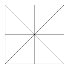
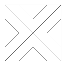
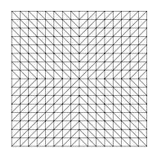
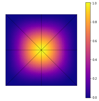
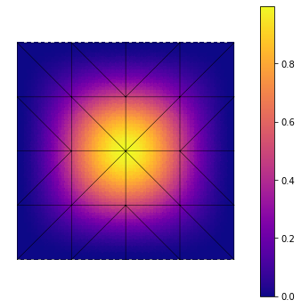
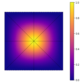
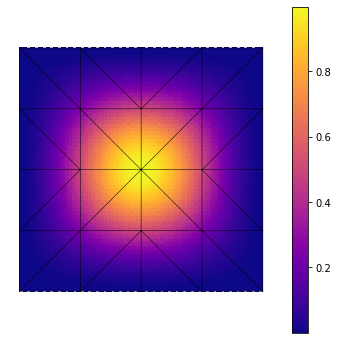
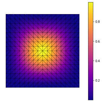
Figure 2: Mesh sequence (top row) and the deflections computed with the classical method (middle row) and Nitsche’s method (bottom row). The source code for reproducing these results is available in [11].

Table 1: Pointwise deflections in the mid point of the clamped square plate.

$h$	Nitsche, $u_{h}(1/2,1/2)$	traditional, $u_{h}(1/2,1/2)$
$0.7071068$	$1.0058542$	$1.0109074$
$0.3535534$	$0.9999617$	$1.000042$
$0.1767767$	$0.9999951$	$0.9999951$
$0.0883883$	$0.9999999$	$0.9999999$

Continuing only with the Nitsche method, we calculate the discrete norm $\|u-u_{h}\|_{h}$ and the following elementwise a posteriori error indicator:

$$E_{K}(u_{h})= \,h_{K}^{2}\|D\Delta^{2}u_{h}-f\|_{0,K}+\frac{1}{2}h_{K}^{3/2}\|\llbracket V_{n}(u_{h})\rrbracket\|_{0,\partial K}$$

$$+\frac{1}{2}h_{K}^{1/2}\|\llbracket M_{nn}(u_{h})\rrbracket\|_{0,\partial K}+h^{3/2}_{K}\|u_{h}\|_{0,\partial K\cap\partial\Omega}$$

$$+h^{1/2}_{K}\left\|\frac{\partial u_{h}}{\partial\boldsymbol{n}}\right\|_{0,\partial K\cap\partial\Omega}+h_{K}^{-1}\sum_{i=1}^{4}u_{h}(c_{i})\chi_{K}(c_{i}),$$

where

(6.1) $$\chi_{K}(x)=\begin{cases}1&\text{if $x\in K$},\\ 0&\text{otherwise}.\end{cases}$$

The results are summarized in Table 2. We observe that the convergence rates are consistent with the expected rate $\mathcal{O}(h^{4})$ for fifth degree polynomials and regular solutions. Moreover, the error indicator converges with similar rates as the true error which is also a consequence of Theorems 5.9 and 5.

Table 2: Convergence of the error and the error estimator.

$h$	$\|u-u_{h}\|_{h}$	rate		$\sqrt{\sum_{K\in\mathcal{C}_{h}}E_{K}^{2}(u_{h})}$	rate
$0.7071068$	$2.5089$			$24.8552837$
$0.3535534$	$0.1935319$	$3$	$.69642$	$2.3444698$	$3$	$.40622$
$0.1767767$	$0.0130669$	$3$	$.88858$	$0.161088$	$3$	$.86334$
$0.0883883$	$7.6500122\cdot 10^{-4}$	$4$	$.09433$	$0.0103163$	$3$	$.96483$

6.2 Plate supported at the corners

Next we consider the same problem with loading $f=1$ and $\varepsilon^{c}_{i}=0$, $\varepsilon^{r}_{i}=\varepsilon^{v}_{i}=\infty$, $g^{v}_{i}=g^{r}_{i}=g^{c}_{i}=0$, $i=1,\dots,4$, i.e. the deflection is prevented only at the corners of the plate. We investigate the convergence rate of the error indicator

$$E_{K}(u_{h})= \,h_{K}^{2}\|D\Delta^{2}u_{h}-1\|_{0,K}+\frac{1}{2}h_{K}^{3/2}\|\llbracket V_{n}(u_{h})\rrbracket\|_{0,\partial K}$$

$$+\frac{1}{2}h_{K}^{1/2}\|\llbracket M_{nn}(u_{h})\rrbracket\|_{0,\partial K}+h^{3/2}_{K}\|V_{n}(u_{h})\|_{0,\partial K\cap\partial\Omega}$$

$$+h^{1/2}_{K}\left\|M_{nn}(u_{h})\right\|_{0,\partial K\cap\partial\Omega}+h_{K}^{-1}\sum_{i=1}^{4}u_{h}(c_{i})\chi_{K}(c_{i})$$

as a function of the number of degrees-of-freedom $N$ with uniform and adaptive mesh refinement strategies. The results shown in Figure 3 indicate that an adaptive refinement based on the error indicator $E_{K}(u_{h})$ successfully recovers the convergence rate $\mathcal{O}(N^{-2})$.

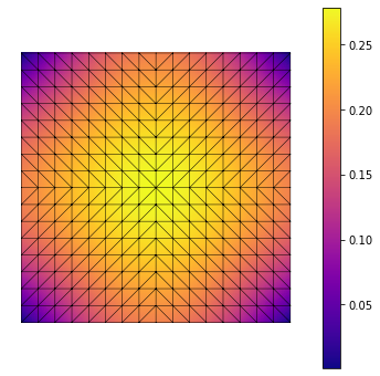
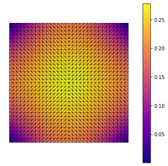
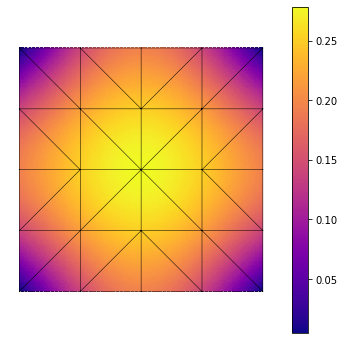
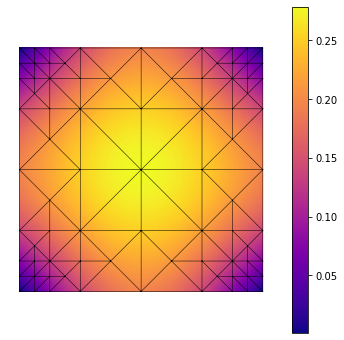
Figure 3: The first four meshes in the uniform (top row) and the adaptive (middle row) mesh sequences with the corresponding solutions and the a posteriori error estimator (bottom row) plotted as a function of the number of degrees-of-freedom $N$ with $\gamma=10^{-3}$. The source code for reproducing the example is available in [12].

6.3 Elastic support with applied loads at the boundaries

As the final example, we consider the square plate problem with $\nu=0$, $\varepsilon^{v}_{i}=1$, $\varepsilon^{c}_{i}=\infty$, the loading $f=0$, and

(6.2) $$g^{v}_{i}=g^{v}(y)=\begin{cases}1&\text{if $y<3/4$},\\ 0&\text{otherwise},\end{cases}\qquad g^{r}_{i}=g^{r}(y)=\begin{cases}10&\text{if $y<1/4$},\\ 0&\text{otherwise},\end{cases}$$

for each $i=1,\dots,4$. Our aim is to compare the adaptive meshes resulting from the Nitsche method and the classical method when $\varepsilon^{r}_{i}=\varepsilon^{r}=10^{-k}$, $k=0,2,4,6$, $i=1,\dots,4$. The error indicator for Nitsche’s method reads as

$$E_{K}(u_{h})= \,h_{K}^{2}\|D\Delta^{2}u_{h}\|_{0,K}+\frac{1}{2}h_{K}^{3/2}\|\llbracket V_{n}(u_{h})\rrbracket\|_{0,\partial K}+\frac{1}{2}h_{K}^{1/2}\|\llbracket M_{nn}(u_{h})\rrbracket\|_{0,\partial K}$$

$$+\frac{h^{3/2}_{K}}{1+h_{K}^{3}}\|V_{n}(u_{h})-g^{v}+u_{h}\|_{0,\partial K\cap\partial\Omega}$$

$$+\frac{h_{K}^{1/2}}{\varepsilon^{r}+h_{K}}\left\|\varepsilon^{r}(M_{nn}(u_{h})-g^{r})-\frac{\partial u_{h}}{\partial\boldsymbol{n}}\right\|_{0,\partial K\cap\partial\Omega}$$

$$+h_{K}\sum_{i=1}^{4}\llbracket M_{ns}(u_{h})\rrbracket|_{c_{i}}\chi_{K}(c_{i}).$$

The error indicator for the classical method is

$$E_{K}(u_{h})= \,h_{K}^{2}\|D\Delta^{2}u_{h}\|_{0,K}+\frac{1}{2}h_{K}^{3/2}\|\llbracket V_{n}(u_{h})\rrbracket\|_{0,\partial K}+\frac{1}{2}h_{K}^{1/2}\|\llbracket M_{nn}(u_{h})\rrbracket\|_{0,\partial K}$$

$$+h^{3/2}_{K}\|V_{n}(u_{h})-g^{v}+u_{h}\|_{0,\partial K\cap\partial\Omega}$$

$$+h_{K}^{1/2}\left\|M_{nn}(u_{h})-g^{r}-\frac{1}{\varepsilon^{r}}\frac{\partial u_{h}}{\partial\boldsymbol{n}}\right\|_{0,\partial K\cap\partial\Omega}.$$

The resulting adaptive meshes are presented in Figure 4. The results show that the classical method can lead to overrefinement in the case of stiff elastic supports.

$\varepsilon^{r}=1$
  
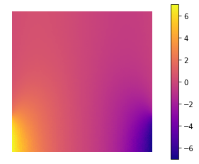
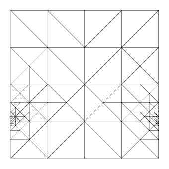
$\varepsilon^{r}=10^{-2}$

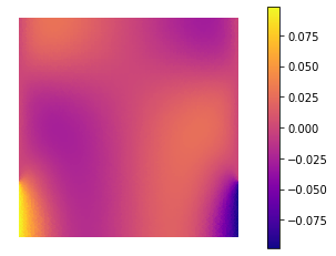
$\varepsilon^{r}=10^{-4}$

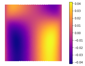
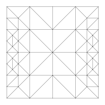
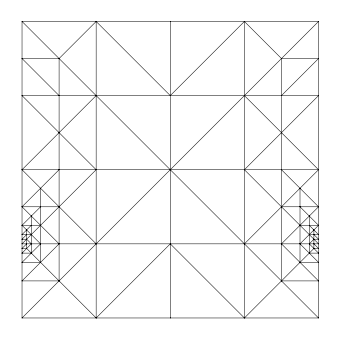
$\varepsilon^{r}=10^{-6}$

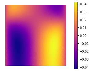
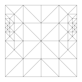
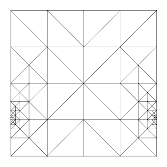
Figure 4: (Left column.) The derivative of the deflection $u$ with respect to $x$. The presence of a singularity at $y=1/4$—due to a jump in the applied normal moment—is evident in the two topmost figures but not so much in the two bottom figures. (Middle column.) The meshes corresponding to the fifth adaptive refinement in the Nitsche method for different values of $\varepsilon^{r}$. If $\varepsilon^{r}$ is small enough, the estimators successfully discard the lower singularity at $y=1/4$ and focus instead on the singularity at $y=3/4$ caused by a jump in the Kirchhoff shear force. (Right column.) The meshes corresponding to the fifth adaptive refinement in the classical method for different values of $\varepsilon^{r}$. The estimators of the classical method remain dominant near the lower singularity for small values of $\varepsilon^{r}$ due to the estimators scaling as $\mathcal{O}(1/\varepsilon^{r})$. The source code for reproducing the example is available in [13].

References

- [1] D. Arnold and S. Walker, The Hellan-Herrmann-Johnson method with curved elements, (2019), https://arxiv.org/abs/1909.09687.
- [2] L. Beirão da Veiga, J. Niiranen, and R. Stenberg, A family of finite elements for Kirchhoff plates. I. Error analysis, SIAM J. Numer. Anal., 45 (2007), pp. 2047–2071, https://doi.org/10.1137/06067554X.
- [3] L. Beirão da Veiga, J. Niiranen, and R. Stenberg, A family of finite elements for Kirchhoff plates. II. Numerical results, Comput. Methods Appl. Mech. Engrg., 197 (2008), pp. 1850–1864, https://doi.org/10.1016/j.cma.2007.11.015.
- [4] J. Blaauwendraad, Plates and Fem, Springer Netherlands, 2010, https://doi.org/10.1007/978-90-481-3596-7.
- [5] S. Brenner, M. Neilan, and L.-Y. Sung, Isoparametric Interior Penalty Methods for Plate Bending Problems on Smooth Domains, Calcolo, 50 (2012), pp. 35–67, https://doi.org/10.1007/s10092-012-0057-1.
- [6] P. G. Ciarlet, The finite element method for elliptic problems, vol. 4 of Studies in Mathematics and its Applications, North-Holland Publishing Co., 1978.
- [7] P. G. Ciarlet, The Finite Element Method for Elliptic Problems, Society for Industrial and Applied Mathematics, 2002, https://doi.org/10.1137/1.9780898719208.
- [8] V. Domínguez and F.-J. Sayas, Algorithm 884: A Simple Matlab Implementation of the Argyris Element, ACM Trans. Math. Softw., 35 (2008), https://doi.org/10.1145/1377612.1377620.
- [9] K. Feng and Z.-C. Shi, Mathematical theory of elastic structures, Springer-Verlag, Berlin; Science Press, Beijing, 1996.
- [10] K. Friedrichs, Die Randwert-und Eigenwertprobleme aus der Theorie der elastischen Platten. (Anwendung der direkten Methoden der Variationsrechnung), Math. Ann., 98 (1928), pp. 205–247, https://doi.org/10.1007/BF01451590.
- [11] T. Gustafsson, kinnala/kirchhoff-nitsche-ex1 v1, 2020, https://doi.org/10.5281/zenodo.3925365.
- [12] T. Gustafsson, kinnala/kirchhoff-nitsche-ex2 v1, 2020, https://doi.org/10.5281/zenodo.3925367.
- [13] T. Gustafsson, kinnala/kirchhoff-nitsche-ex3 v1, 2020, https://doi.org/10.5281/zenodo.3925375.
- [14] T. Gustafsson and G. D. McBain, kinnala/scikit-fem 1.0.0, 2020, https://doi.org/10.5281/zenodo.3773438.
- [15] T. Gustafsson, R. Stenberg, and J. Videman, A Posteriori Estimates for Conforming Kirchhoff Plate Elements, SIAM J. Sci. Comput., 40 (2018), pp. A1386–A1407, https://doi.org/10.1137/17m1137334.
- [16] M. Juntunen and R. Stenberg, Nitsche’s method for general boundary conditions, Math. Comput., 78 (2009), pp. 1353–1374.
- [17] G. Kirchhoff, Über das Gleichgewicht und die Bewegung einer elastischen Scheibe, J. Reine. Angew. Math., 40 (1850), pp. 51–88.
- [18] A. Love, XVI. The small free vibrations and deformation of a thin elastic shell, Philos. T. Roy. Soc. A, (1888), pp. 491–546.
- [19] N. Lüthen, M. Juntunen, and R. Stenberg, An improved a priori error analysis of Nitsche’s method for Robin boundary conditions, Numer. Math., 138 (2018), pp. 1011–1026, https://doi.org/10.1007/s00211-017-0927-1.
- [20] J. Nečas and I. Hlaváček, Mathematical Theory of Elastic and Elasto-Plastic Bodies: An Introduction, vol. 3 of Studies in Applied Mechanics, Elsevier Scientific Publishing Co., Amsterdam-New York, 1980.
- [21] J. A. Nitsche, Über ein Variationsprinzip zur Lösung von Dirichlet-Problemen bei Verwendung von Teilräumen, die keinen Randbedingungen unterworfen sind, in Abhandlungen aus dem mathematischen Seminar der Universität Hamburg, vol. 36, Springer, 1971, pp. 9–15.
- [22] Y. Renard and K. Poulios, GetFEM: Automated FE modeling of multiphysics problems based on a generic weak form language, (2020), https://hal.archives-ouvertes.fr/hal-02532422 .
- [23] J. Valdman, MATLAB Implementation of C1 Finite Elements: Bogner-Fox-Schmit Rectangle, in Parallel Processing and Applied Mathematics, R. Wyrzykowski, E. Deelman, J. Dongarra, and K. Karczewski, eds., Cham, 2020, Springer International Publishing, pp. 256–266.
- [24] J. Zhang, C. Zhou, S. Ullah, Y. Zhong, and R. Li, Accurate Bending Analysis of Rectangular Thin Plates With Corner Supports By a Unified Finite Integral Transform Method, Acta Mech., 230 (2019), pp. 3807–3821.
- [25] O. C. Zienkiewicz and R. L. Taylor, The Finite Element Method. Volume 2: Solid Mechanics, Butterworth-Heinemann, Oxford, fifth ed., 2000.