Cobalt and copper abundances in 56 Galactic bulge red giants

Abstract

Context. The Milky Way bulge is an important tracer of the early formation and chemical enrichment of the Galaxy. The abundances of different iron-peak elements in field bulge stars can give information on the nucleosynthesis processes that took place in the earliest supernovae. Cobalt (Z=27) and copper (Z=29) are particularly interesting.

Aims. We aim to identify the nucleosynthesis processes responsible for the formation of the iron-peak elements Co and Cu.

Methods. We derived abundances of the iron-peak elements cobalt and copper in 56 bulge giants, 13 of which were red clump stars. High-resolution spectra were obtained using FLAMES-UVES at the ESO Very Large Telescope by our group in 2000-2002, which appears to be the highest quality sample of high-resolution data on bulge red giants obtained in the literature to date. Over the years we have derived the abundances of C, N, O, Na, Al, Mg; the iron-group elements Mn and Zn; and neutron-capture elements. In the present work we derive abundances of the iron-peak elements cobalt and copper. We also compute chemodynamical evolution models to interpret the observed behaviour of these elements as a function of iron.

Results. The sample stars show mean values of [Co/Fe]$\sim$0.0 at all metallicities, and [Cu/Fe]$\sim$0.0 for [Fe/H]$\geq$-0.8 and decreasing towards lower metallicities with a behaviour of a secondary element.

Conclusions. We conclude that [Co/Fe] varies in lockstep with [Fe/H], which indicates that it should be produced in the alpha-rich freezeout mechanism in massive stars. Instead [Cu/Fe] follows the behaviour of a secondary element towards lower metallicities, indicating its production in the weak s-process nucleosynthesis in He-burning and later stages. The chemodynamical models presented here confirm the behaviour of these two elements (i.e. [Co/Fe] vs. [Fe/H]$\sim$constant and [Cu/Fe] decreasing with decreasing metallicities).

1 Introduction

The detailed study of element abundances in the Milky Way bulge can inform on the chemical enrichment processes in the Galaxy, and on the early stages of the Galaxy formation. Field stars in the Galactic bulge are old (Renzini et al. 2018, and references therein), and bulge globular clusters, in particular the moderately metal-poor ones, are very old (e.g. Kerber et al. 2018, 2019, Oliveira et al. 2020). The study of bulge stars can therefore provide hints on the chemical enrichment of the earliest stellar populations in the Galaxy. Abundance ratio indicators have been extensively used in the literature and interpreted in terms of nucleosynthesis typical of different types of supernovae and chemical evolution models. The studies are most usually based on the alpha-elements O, Mg, Ca, and Si, and on Al and Ti, which behave like alpha-elements that are enhanced in metal-poor stars (e.g. Mishenina et al. 2002, Cayrel et al. 2004, Lai et al. 2008), in the Galactic bulge (e.g. McWilliam 2016, Friaça & Barbuy 2017), and elliptical galaxies (e.g. Matteucci & Brocato 1990). The alpha-element enhancement in old stars is due to a fast chemical enrichment by supernovae type II (SNII). Other independent indicators have so far been less well studied, notably iron-peak elements, s-elements, and r-elements. Ting et al. (2012) aimed to identify which groups of elements are independent indicators of the supernova type that produced them. Their study reveals two types of SNII: one that produces mainly $\alpha$-elements and one that produces both $\alpha$-elements and Fe-peak elements with a large enhancement of heavy Fe-peak elements, which may be the contribution from hypernovae. This shows the importance of deriving Fe-peak element abundances.

The Fe-peak elements have atomic numbers in the range 21 $\leq$ Z $\leq$ 32. The lower iron group includes Sc, Ti, V, Cr, Mn, and Fe and the upper iron-group contains Co, Ni, Cu, and Zn, and probably also Ga and Ge. Most of these elements vary in lockstep with Fe as a function of metallicity, with the exception of Sc, Ti, Mn, Cu, and Zn, and perhaps Co (e.g. Gratton 1989, Nissen et al. 2000, Sneden et al. 1991, Cayrel et al. 2004, Ishigaki et al. 2013, da Silveira et al. 2018). This occurs because most Fe is produced in SNIa, whereas some of the iron-peak elements, in particular Co and Cu, are well produced in massive stars (Sukhbold et al. 2016, and references therein).

We previously analysed the iron-peak elements Mn and Zn (Barbuy et al. 2013, 2015, da Silveira et al. 2018) in the same sample of field stars studied in the present work, as well as Sc, V, Cu, Mn, and Zn in bulge globular cluster stars (Ernandes et al. 2018). In this paper we analyse abundances of the iron-peak elements cobalt and copper. These two elements, and copper in particular, deserve attention because the nucleosynthesis processes that produce them have been discussed over the years in the literature. The production of Cu in massive stars as a secondary product was only challenged by Mishenina et al. (2002), who argued that a sum of a secondary and a primary process would be needed to explain the behaviour of [Cu/Fe] versus [Fe/H] in metal-poor stars. Bisterzo et al. (2004) concluded that most Cu derives from a secondary weak-s process in massive stars; a small primary contribution of $\sim$5% in the Sun would be due to the decay of ^63,65Zn, and this becomes dominant for [Fe/H]$<$-2.0. On the other hand, asymptotic giant branch (AGB) stars and SNIa contribute little to Cu. Pignatari et al. (2010) presented nucleosynthesis calculations showing an increased production of Cu from a weak-s process in massive stars. Romano & Matteucci (2007) concluded that Cu enrichment is due to a primary contribution from explosive nucleosynthesis in SNII, and a weak s-process in massive stars. Lai et al. (2008) data on halo stars agreed with these models.

According to Woosley & Weaver (1995, hereafter WW95), Limongi et al. (2003), and Woosley et al. (2002), the upper iron-group elements are mainly synthesized in two processes: either neutron capture on iron-group nuclei during He burning and later burning stages (also called the weak s-component); or the $\alpha$-rich freezeout in the deepest layers. Both cobalt and copper are produced as primary elements in the $\alpha$-rich freezeout and as secondary elements in the weak s-process in massive stars. The relative efficiency of these two contributions to the nucleosynthesis of Co and Cu can be tested by deriving their abundances in the Galaxy. Abundances gathered so far, in the Galactic bulge in particular, indicate that copper behaves as a secondary element, therefore with a significant contribution from the weak s-process. Cobalt, which appears to vary in lockstep with Fe, seems instead to be mostly contributed from the $\alpha$-rich freezeout mechanism (Barbuy et al. 2018, Woosley, private communication).

Very few previous analyses of iron-peak elements in Galactic bulge stars are available in the literature. For copper, Johnson et al. (2014) and Xu et al. (2019) are so far the only available data derived from moderately high-resolution spectra. For cobalt, Johnson et al. (2014) present results from moderately high-resolution spectra, Schultheis et al. (2017) from near-infrared (NIR) spectra, and Lomaeva et al. (2019) from high-resolution spectra.

Our observations are outlined in Sect. 2. In Sect. 3 we list the basic stellar parameters, report atomic constants under study for the lines of Co and Cu, and describe the abundance derivation of Co and Cu. Chemical evolution models are presented in Sect. 4. The results are discussed in Sect. 5, and conclusions are drawn in Sect. 6.

2 Observations

The present data consist of high-resolution spectra of 43 bulge red giants, chosen to have one magnitude brighter than the red clump, from ESO programmes 71.B-0617A and 73.B0074A (PI: A. Renzini) obtained with the FLAMES-UVES spectrograph (Dekker et al. 2000) at the 8.2 m Kueyen Very Large Telescope at the Paranal Observatory of the European Southern Observatory (ESO). The stars were observed in four fields, namely Baade’s Window (BW) (l=1.14^∘, b=-4.2^∘), a field at $\rm b=-6^{\circ}$ (l=0.2^∘, b=$-6^{\circ}$), the Blanco field (l=0^∘, b=$-12^{\circ}$), and a field near NGC 6553 (l=5.2^∘, b=$-3^{\circ}$). Thirteen additional red clump bulge giants were observed in programme GTO 71.B-0196 (PI: V. Hill), as described in Hill et al. (2011).

The mean wavelength coverage is 4800-6800 Å. With the UVES (Ultraviolet and Visual Echelle Spectrograph) standard setup 580, the resolution is R $\sim$ 45 000 for a 1 arcsec slit width, given that the fibres are 1.0” wide. Typical signal-to-noise ratios obtained by considering average values at different wavelengths vary in the range 30 $\leq$ S/N $\leq$ 280 per pixel in the programme stars. Here the analysis is based uniquely on the UVES spectra, but it is noteworthy that the same sample of stars was also observed with the GIRAFFE spectrograph, as part of a larger sample (Zoccali et al. 2008), with the purpose of validating their abundance analysis at the lower resolution (R $\sim$ 22,000) of GIRAFFE.

As described in Zoccali et al. (2006), Lecureur et al. (2007), and Hill et al. (2011), the spectra were reduced using the FLAMES-UVES pipeline, including bias and inter-order background subtraction, flat-field correction, extraction, and wavelength calibration (Ballester et al. 2000).

This sample of stars had the abundances of O, Na, Mg, and Al studied in Zoccali et al. (2006) and Lecureur et al. (2007). The C, N, and O abundances were revised in Friaça & Barbuy (2017). The iron-peak elements Mn and Zn were studied in Barbuy et al. (2013, 2015) and da Silveira et al. (2018), and heavy elements in van der Swaelmen et al. (2016). In summary, the abundances of C, N, O, Na, Mg, Al, Mn, Zn, and heavy elements were derived. González et al. (2011) derived abundances of Mg, Si, Ca, and Ti for a GIRAFFE counterpart of the sample, obtained at R $\sim$ 22 000). Da Silveira et al. (2018) derived O and Zn from GIRAFFE data in two fields.

It is interesting to note that this data set, including both the high-resolution UVES data as well as the moderately high-resolution GIRAFFE data, has become an important reference for bulge studies; from this same ESO programme, Johnson et al. (2014) analysed GIRAFFE data for 156 red giants in the Blanco and near-NGC 6553 fields, and Xu et al. (2019) reanalysed 129 of these same stars. Jönsson et al. (2017) reanalysed UVES spectra of a sub-sample of 33 stars from our sample of 43 red giants, and additionally analysed two other stars, BW-b1 and B2-b8, that were observed but not included in the studies by Zoccali et al. (2006, 2008). A comparison of stellar parameters between Zoccali et al. (2006) and Lecureur et al. (2007) relative to Jönsson et al. (2017) is discussed in da Silveira et al. (2018). The same sub-sample that was reanalysed by Jönsson et al. (2017) was further analysed by Forsberg et al. (2019), Lomaeva et al. (2019), and Grisoni et al. (2020) for different elements, adopting their own stellar parameters. Finally, Schultheis et al. (2017) compared APOGEE (Apache Point Observatory Galactic Evolution Experiment) results with stars in common with Zoccali et al. (2008)’s results for stars observed with GIRAFFE.

3 Abundance analysis

The stellar parameters effective temperature (T_eff), gravity (log g), metallicity ([Fe/H]), and microturbulence velocity (v_t) are adopted from our previous determinations (Zoccali et al. 2006, 2008, Lecureur et al. 2007), which we summarize below.

The VIJKH de-reddened magnitudes were combined to obtain photometric temperatures from V-I, V-J, V-H, and V-K colours. The mean of the four values was used as a first guess for a spectroscopic analysis. Photometric gravity was calculated from the classical relation

$$\log g_{*}=4.44+4\log\frac{T_{*}}{T_{\odot}}+0.4(M_{\rm bol}-4.75)+\log\frac{M_{*}}{M_{\odot}},$$

adopting T_⊙=5770 K, M_∗=0.85 M_⊙, M_bol⊙ = 4.75, and a mean distance of 8 kpc for the Galactic bulge.

The equivalent widths for selected lines of Fe, Na, Mg, Al, Si, Ca, Sc, Ti, and Ni were measured using the code DAOSPEC (Stetson and Pancino 2008). The selection of clean Fe lines and their atomic parameters was compiled using a spectrum of $\mu$ Leo as reference (Lecureur et al. 2007).

The LTE abundance analysis was performed using an updated version of the code ABON2 (Spite 1967) and MARCS models (Gustafsson et al. 2008). Excitation equilibrium was imposed on the Fe I lines in order to refine the photometric T_eff, while photometric gravity was imposed even if ionization equilibrium was not fulfilled.

Elemental abundances were obtained through line-by-line spectrum synthesis calculations. The calculations of synthetic spectra were carried out using the PFANT code described in Barbuy et al. (2018b), where molecular lines of the CN A²$\Pi$-X²$\Sigma$, C₂ Swan A³$\Pi$-X³$\Pi$ and TiO A³$\Phi$-X³$\Delta$ $\gamma,$ and B³$\Pi$-X³$\Delta$ $\gamma$’ systems are taken into account. The MARCS model atmospheres are adopted (Gustafsson et al. 2008).

The abundances derived line-by-line are reported in Table 3. The final mean abundances are given in the last three columns of Table 4, where the final mean values of [Cu/Fe] and [Co/Fe] in LTE and NLTE-corrected are reported.

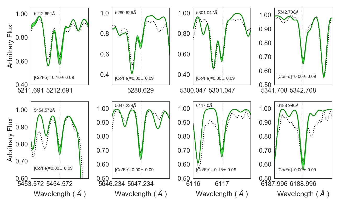
Figure 1: Fits of synthetic spectra to the eight observed lines of Co I in star BWc-4. The dotted line is the observed spectrum. The green lines correspond to the value adopted, and with [Co/Fe]=+0.09 and -0.09.

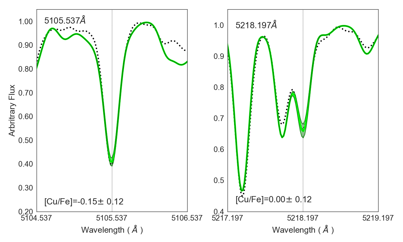
Figure 2: Fits of synthetic spectra to the two observed lines of Cu I in star BL-7. The dotted line is the observed spectrum. The green lines correspond to the value adopted, and with [Cu/Fe]=+0.12 and -0.12.

Figure 1 shows the fit to the eight Co I lines in star BWc-4. Figure 2 shows the fit to the Cu I 5105.537 and 5218.197 Å lines for star BL-7.

3.1 Line parameters: hyperfine structure, oscillator strengths, and solar abundances

We derive cobalt and copper abundances for the 56 sample stars using the lines of Co I and Cu I reported in Table 1. The oscillator strengths and the hyperfine structure (HFS) we adopted are described below.

Cobalt: Co I lines

Cobalt has the unique species ⁵⁹Co (Asplund et al. 2009). The HFS was taken into account by applying the code made available by McWilliam et al. (2013) together with the A and B constants reported in Table 7 that were adopted from Pickering et al. (1996). Cobalt has a nuclear spin I = 7/2. Central wavelengths and excitation potential values from Kurúcz (1993), the oscillator strengths from Kurúcz (1993), NIST (Martin et al. 2002), and VALD (Piskunov et al. 1995), and the final values adopted are presented in Table 1.

Tables 8, 9, and 10 show the HFS components of the Co I lines studied. All these lines were checked by comparing synthetic spectra to high-resolution spectra of the Sun (using the same instrument settings as the present sample of spectra ), Arcturus (Hinkle et al. 2000), and the metal-rich giant star $\mu$ Leo (Lecureur et al. 2007). We adopted the following stellar parameters: effective temperature (T_eff), surface gravity (log g), metallicity ([Fe/H]), and microturbulent velocity (v_t) of (4275 K, 1.55, -0.54, 1.65 km.s^-1) for Arcturus from Meléndez et al. (2003), and (4540 K, 2.3, +0.30, 1.3 km.s^-1) for $\mu$ Leo from Lecureur et al. (2007). The adopted abundances for the Sun, Arcturus, and $\mu$ Leo are reported in Table 2.

Copper: Cu I lines

Copper abundances were derived from the two Cu I lines at 5105 and 5218 Å already employed and described in detail in Ernandes et al. (2018). The 5782 Å line is not available in the UVES spectra. Isotopic fractions of 0.6894 for ⁶³Cu and 0.3106 for ⁶⁵Cu (Asplund et al. 2009), as well as the HFS structure as given in Ernandes et al. (2018), are adopted.

Figures 6 and 7 show the fits to the spectra of the Sun, Arcturus, and $\mu$ Leo. The Cu I atomic parameters and fits to these reference stars were already extensively discussed in Ernandes et al. (2018).

Table 1: Central wavelengths and total oscillator strengths.

species	$\lambda$ (Å)	$\chi_{ex}$ (eV)	gfKurucz	gfNIST	gfVALD	gfadopted
CoI	4749.669	3.053457	-0.321	—	-0.236	-0.321
CoI	5212.691	3.514439	-0.110	-0.11	-0.110	-0.110
CoI	5280.629	3.628984	-0.030	-0.03	-0.030	-0.030
CoI	5301.039	1.710426	-2.000	-1.99	-2.000	-2.000
CoI	5342.695	4.020881	0.690	—	0.741	0.690
CoI	5454.572	4.071888	-0.238	—	+0.238	+0.238
CoI	5647.234	2.280016	-1.560	-1.56	-1.560	-1.560
CoI	6117.000	1.785283	-2.490	-2.49	-2.490	-2.490
CoI	6188.996	1.710426	-2.450	-2.46	-2.450	-2.450
CuI	5105.537	1.389035	-1.516	-1.50	hfs	-1.52
CuI	5218.197	3.816948	0.476	0.264	hfs	+0.124

Table 2: Adopted abundances for the Sun, Arcturus, and $\mu$Leo. References: [1]: Grevesse et al. (1996); Grevesse & Sauval (1998); Asplund et al. (2009); Lodders (2009); [2]: Steffen et al. (2015); [3]: Ramírez & Allende Prieto (2011); [4]: Meléndez et al. (2003) [5]: Barbuy et al. (2015); Friaça & Barbuy (2017); [6]: Smith et al. (2013); [7]: Gratton & Sneden (1990); [8]: Lecureur et al. (2007) [9]: Barbuy et al. (2014) [10]: Smith & Ruck (2000) [11]: Scott et al. (2015a,b) [12]: McWilliam et al. (2013)

El.	Z	A(X)⊙	A(X)Arcturus	A(X)μLeo
Fe	26	7.50 [1]	6.96 [4]	7.80 [5]
C	6	8.55 [1]	7.79 [8]	8.55 [5]
N	7	7.97 [1]	7.65 [8]	8.83 [5]
O	8	8.77 [2]	8.62 [9]	8.97 [5]
Na	11	6.33 [1]	5.90 [3]	7.07 [10]
Mg	12	7.58 [1]	7.41 [3]	7.91 [10]
Al	13	6.47 [1]	6.26 [3]	6.90 [6]
Si	14	7.55 [1]	7.34 [11]	8.02 [7]
K	19	5.12 [1]	4.99 [3]	5.63 [6]
Ca	20	6.36 [1]	5.94 [3]	6.62 [6]
Sc	21	3.17 [1]	2.86 [5]	3.34 [7]
Ti	22	5.02 [1]	4.74 [13]	5.39 [10]
V	23	4.00 [1]	3.58 [3]	4.34 [7]
Cr	24	5.67 [1]	5.08 [3]	5.97 [7]
Mn	25	5.39 [1]	4.71 [12]	5.70 [7]
Co	27	4.92 [1]	5.11 [3]	4.93 [7]
Ni	28	6.25 [1]	5.77 [3]	6.60 [10]
Cu	29	4.21 [1]	4.09 [3]	4.46 [10]
Zn	30	4.60 [1]	4.06 [5]	4.80 [5]

3.2 Non-local thermodynamic equilibrium corrections

We applied the NLTE corrections for each cobalt line following the same method used by Kirby et al. (2018), with the formalism of Bergemann & Cescutti (2010) and Bergemann et al. (2010) . The derivation of corrections from the online code made available requires the choice of atmospheric model, inclusion of stellar parameters of each star, and the line list, followed by the atomic number (Z) under study. The corrections so derived line-by-line for the Co abundances are reported in Table 11, and final NLTE-corrected Co abundance values are given in Table 4.

3.3 Uncertainties

As with our previous papers regarding this sample of spectra, and given that the final adopted atmospheric parameters for the program stars were based on Fe I and Fe II lines together with photometric gravities, we have adopted their estimated uncertainties in the atmospheric parameters (i.e. $\pm$ 100 K for temperature, $\pm$ 0.20 for surface gravity, and $\pm$ 0.20 kms^-1 for microturbulent velocity). In Table 5 we compute Co and Cu abundances for the metal-rich star B6-f8 and the metal-poor star BW-f8 by changing their parameters by these amounts. The errors computed by adopting models with $\Delta$T_eff=+100K, $\Delta$log g=+0.2, and $\Delta$v_t=+0.2 km.s^-1, as well as final errors, are shown in Table 5.

For comparison purposes, we have listed the stars that were also analysed by Johnson et al. (2014) and Jönsson et al. (2016) in Table 6, reporting the respective stellar parameters they adopted. Johnson et al. (2014) analysed their corresponding GIRAFFE spectra, while Jönsson et al. (2016) reanalysed the same UVES data as Zoccali (2006, 2008) and Lecureur et al. (2007); these data and stellar parameters are the same as given in Lomaeva et al. (2019).

The differences in stellar parameters between the present ones adopted from Zoccali et al. (2006, 2008), Lecureur et al. (2007), and the reanalysis by Jönsson et al. (2017) were discussed in da Silveira et al. (2018). As reported in Sect. 3, the present parameters (see Sect. 3) were obtained by applying excitation equilibrium imposed on the Fe I lines in order to refine the photometric T_eff, and photometric gravity was imposed.

The Lomaeva et al. (2019) parameters, adopted from Jönsson et al. (2017), were obtained by using the software Spectroscopy Made Easy (SME; Valenti & Piskunov 1996). The SME software simultaneously fits stellar parameters and/or abundances by fitting calculated synthetic spectra to an observed spectrum. All the stellar parameters (T_eff , log g, [Fe/H], and v_t) were derived simultaneously using relatively weak, unblended Fe I, Fe II , and Ca I lines and gravity-sensitive Ca I-wings.

In the mean, the differences in parameters amount to $\Delta$T_eff(Jönsson+17-Zoccali+06)=-94 K in effective temperatures and $\Delta$log g(Jönsson+17-Zoccali+06)=+0.46 in gravities. The gravities adopted by Jönsson et al. (2017) are possibly too high because the sample stars were chosen to have one magnitude brighter than the red clump or horizontal branch. It is well known that the red clump stars have rather homogeneous gravity values of log g$\sim$2.2 that can go up to log g$\sim$2.5 at most, depending on metallicity (Girardi 2016), and should be around log g$\sim$2.3 for the stellar parameters of the present metallicities. Therefore, it appears natural that red giants located at one magnitude above the red clump should have gravities around log g$\sim$2.0 (or lower). On the other hand, the patchy extinction towards the bulge might arguably accommodate larger gravities for the sample stars, as assumed by Jönsson et al. (2017). In any case, we prefer to keep the parameters from our group for the sake of homogeneity of elemental abundances between this paper and the previous ones. Furthermore, since we have 56 stars, including 33 in common with Jönsson et al. (2017), it is also important to have an internal consistency in the analysis of the 56 stars.

A check of lines used by each author can explain some differences in the results, as follows. (i) Comparison of lines used for cobalt: Johnson et al. (2014) used the Co I 5647.23 and 6117.00 Å lines. Lomaeva et al. (2019) only used the UVES spectra from the red arm and relied on the Co I 6005.020, 6117.000, 6188.996, and 6632.430 Å. We have used lines from both the red arm and the blue arm spectra, as listed in Table 1; (ii) Comparison of lines used for copper: Johnson et al. (2014) and Xu et al. (2019) used the same Cu I 5782.11 Å line for the same stars, which is a well-known suitable line with identified HFS structure.

Table 3: LTE abundances of Co and Cu derived in the present work.

Star	[Fe/H]	[Cu/Fe]	[Cu/Fe]	[Co/Fe]	[Co/Fe]	[Co/Fe]	[Co/Fe]	[Co/Fe]	[Co/Fe]	[Co/Fe]	[Co/Fe]
		5105.5374 Å	5218.1974 Å	5212.691 Å	5280.629 Å	5301.047 Å	5342.708 Å	5454.572 Å	5647.234 Å	6117.000 Å	6188.996 Å
B6-b1	0.07	-0.30	-0.10	-0.15	-0.25	-0.30	-0.30	-0.30	-0.15	-0.15	0.00
B6-b2	-0.01	-0.15	0.20	-0.20	+0.00	+0.00	-0.30	-0.25	-0.25	+0.00	-0.20
B6-b3	0.10	0.05	0.00	-0.20	0.00	0.00	-0.15	-0.10	0.00	0.00	0.05
B6-b4	-0.41	0.00	-0.15	-0.15	-0.15	0.00	-0.15	0.00	0.00	0.00	0.00
B6-b5	-0.37	0.35	-0.10	0.00	0.00	-0.15	-0.15	0.00	0.00	-0.15	+0.05
B6-b6	0.11	-0.05	0.00	-0.15	0.00	-0.10	-0.10	-0.15	-0.15	-0.10	+0.10
B6-b8	0.03	-0.30	0.00	-0.28	0.00	-0.30	-0.30	-0.30	-0.10	-0.30	-0.05
B6-f1	-0.01	-0.30	-0.10	-0.15	0.00	-0.15	-0.30	-0.15	-0.10	-0.30	0.00
B6-f2	-0.51	-0.30	-0.10	0.00	0.00	—	0.00	-0.15	0.00	-0.30	—
B6-f3	-0.29	0.10	0.00	0.00	0.00	0.00	0.00	-0.10	+0.10	0.00	+0.10
B6-f5	-0.37	-0.30	0.15	-0.10	0.00	0.00	-0.15	-0.15	-0.05	0.00	+0.15
B6-f7	-0.42	-0.35	0.00	0.00	0.00	0.00	0.00	0.00	0.00	0.00	0.00
B6-f8	0.04	0.30	-0.10	0.00	0.00	+0.10	0.00	-0.15	+0.05	-0.15	+0.08
BW-b2	0.22	—	-0.15	0.00	0.00	-0.15	—	-0.20	-0.20	-0.25	0.00
BW-b4	0.07	—	-0.30	-0.20	-0.10	-0.30	+0.05	-0.30	-0.15	+0.15	-0.15
BW-b5	0.17	—	-0.35	0.00	0.00	-0.05	-0.10	0.00	0.00	0.00	0.00
BW-b6	-0.25	—	-0.30	0.00	-0.05	-0.15	-0.10	0.00	0.00	-0.15	0.00
BW-b7	0.10	—	-0.25	-0.30	0.00	-0.30	0.00	-0.30	-0.30	-0.15	-0.10
BW-f1	0.32	-0.40	-0.40	0.00	—	0.00	-0.30	0.00	0.00	0.00	0.00
BW-f4	-1.21	-1.00	-0.60	—	—	—	0.00	0.00:	0.00:	0.00	0.00
BW-f5	-0.59	0.00	-0.30	+0.05	0.00	-0.30	0.00	-0.15	0.00	-0.10	0.00
BW-f6	-0.21	—	-0.50	0.00	0.00	- 0.10	-0.15	-0.05	0.00	0.00	+0.30
BW-f7	0.11	—	—	-0.12	0.00	-0.30	—	-0.30	-0.30	-0.25	0.00
BW-f8	-1.27	-0.70	-0.60	0.00:	—	—	0.00	+0.30	0.00	-0.10:	—
BL-1	-0.16	0.00	0.10	0.00	+0.15	+0.35	+0.30	0.00	+0.30	-0.15	0.00
BL-3	-0.03	0.10	-0.30	0.00	0.00	0.00	+0.05	0.00	+0.05	-0.25	0.00
BL-4	0.13	0.30	0.15	0.00	0.00	+0.10	-0.10	-0.10	+0.12	-0.15	+0.12
BL-5	0.16	0.00	0.00	0.00	0.00	0.00	-0.15	-0.15	-0.15	-0.15	0.00
BL-7	-0.47	0.15	0.00	+0.05	+0.10	+0.10	+0.15	+0.10	+0.10	-0.10	-0.05
B3-b1	-0.78	—	—	+0.10	—	—	—	—	+0.30	-0.30	-0.15
B3-b2	0.18	0.00	-0.30	-0.22	-0.20	+0.15	0.00	-0.20	0.00	-0.18	-0.25
B3-b3	0.18	—	—	-0.07	0.00	+0.10	+0.30	0.00	0.00	-0.25	-0.05
B3-b4	0.17	0.05	-0.30	-0.12	+0.15	-0.05	-0.20	-0.10	+0.25	0.00	-0.07
B3-b5	0.11	0.30	-0.20	-0.10	-0.10	-0.10	0.00	0.00	+0.10	-0.30	+0.05
B3-b7	0.20	0.30	-0.05	0.00	+0.25	0.00	0.00	-0.15	0.00	-0.10	0.00
B3-b8	-0.62	0.20	0.00	0.00	0.00	0.00	0.00	0.00	0.00	-0.03	0.00
B3-f1	0.04	-0.05	-0.20	-0.10	+0.15	-0.30	0.00	-0.10	+0.20	-0.30	0.00
B3-f2	-0.25	0.30	0.30	0.00	-0.20	+0.25	0.00	-0.25	+0.30	0.00	0.00
B3-f3	0.06	-0.30	0.30	-0.23	0.00	0.00	+0.15	-0.15	-0.15	-0.30	-0.05
B3-f4	0.09	-0.40	0.00	—	-0.30	0.00	0.00	0.00	-0.15	-0.30	+0.05
B3-f5	0.16	-0.40	-0.40	-0.15	0.00	-0.30	0.00	+0.15	-0.15	0.00	+0.20
B3-f7	0.16	0.00	0.00	-0.10	+0.15	-0.30	0.00	-0.30	0.00	-0.30	+0.25
B3-f8	0.20	0.50	0.30	-0.10	-0.10	-0.05	-0.07	-0.20	+0.10	0.00	+0.25
BWc-1	0.09	0.00	0.00	-0.10	0.00	0.00	0.00	-0.05	0.00	+0.10	0.00
BWc-2	0.18	-0.60	-0.60	-0.30	0.00	-0.15	—	-0.10	-0.30	-0.30	-0.20
BWc-3	0.28	0.35	0.00	-0.20	0.00	0.00	0.00	-0.30	+0.12	-0.20	0.00
BWc-4	0.05	-0.30	-0.10	-0.10	0.00	0.00	0.00	0.00	0.00	-0.15	0.00
BWc-5	0.42	0.00	-0.20	0.00	0.00	0.00	0.00	-0.25	+0.15	-0.20	+0.20
BWc-6	-0.25	0.30	-0.30	0.00	0.00	0.00	0.00	—	+0.15	-0.08	0.00
BWc-7	-0.25	-0.30	0.00	0.00	+0.10	0.00	0.00	-0.30	+0.10	-0.25	—
BWc-8	0.37	0.00	-0.10	-0.18	-0.12	0.00	0.00	-0.15	-0.15	-0.20	0.00
BWc-9	0.15	0.30	0.30	0.00	0.00	0.00	0.00	0.00	-0.15	-0.15	+0.15
BWc-10	0.07	-0.30	-0.30	-0.15	0.00	0.00	0.00	-0.15	-0.10	-0.30	-0.05
BWc-11	0.17	0.00	-0.30	0.00	0.00	0.00	0.00	—	-0.05	—	-0.30
BWc-12	0.23	-0.35	0.00	-0.18	0.00	-0.05	-0.20	0.00	0.00	-0.15	0.00
BWc-13	0.36	-0.20	-0.30	—	-0.05	0.00	0.00	—	0.00	—	-0.20

Table 4: Atmospheric parameters and radial velocities adopted from Zoccali et al. (2006) and Lecureur et al. (2007), and resulting Co and Cu abundances.

Star	OGLE no.	$\alpha$(J2000)	$\delta$(J2000)	Teff	logg	[Fe/H]	vt	vr	vhelio	[Cu/Fe]LTE	[Co/Fe]LTE	[Co/Fe]NLTE
				[K]			[kms-1]	[kms-1]	[kms-1]
B6-b1	29280c3	18 09 50.480	-31 40 51.61	4400	1.8	0.07	1.6	-88.3	11.59	-0.20	-0.20	-0.07
B6-b2	83500c6	18 10 33.980	-31 49 09.15	4200	1.5	-0.01	1.4	17.0	11.66	0.03	-0.15	-0.04
B6-b3	31220c2	18 10 19.060	-31 40 28.19	4700	2.0	0.10	1.6	-145.8	11.64	0.03	-0.05	0.08
B6-b4	60208c7	18 10 07.770	-31 52 41.36	4400	1.9	-0.41	1.7	-20.3	11.61	-0.08	-0.06	0.03
B6-b5	31090c2	18 10 37.380	-31 40 29.14	4600	1.9	-0.37	1.3	-4.2	11.67	0.13	-0.05	0.06
B6-b6	77743c7	18 09 49.100	-31 50 07.66	4600	1.9	0.11	1.8	44.1	11.58	-0.03	-0.08	0.05
B6-b8	108051c7	18 09 55.950	-31 45 46.33	4100	1.6	0.03	1.3	-110.3	11.59	-0.15	-0.20	-0.11
B6-f1	23017c3	18 10 04.460	-31 41 45.31	4200	1.6	-0.01	1.5	38.4	10.95	-0.20	-0.14	-0.03
B6-f2	90337c7	18 10 11.510	-31 48 19.28	4700	1.7	-0.51	1.5	-98.5	10.96	-0.20	-0.08	0.05
B6-f3	21259c2	18 10 17.720	-31 41 55.20	4800	1.9	-0.29	1.3	90.2	10.97	0.05	+0.01	0.14
B6-f5	33058c2	18 10 41.510	-31 40 11.88	4500	1.8	-0.37	1.4	22.1	11.02	-0.08	-0.04	0.06
B6-f7	100047c6	18 10 52.300	-31 46 42.18	4300	1.7	-0.42	1.6	-10.4	11.03	-0.18	0.00	0.09
B6-f8	11653c3	18 09 56.840	-31 43 22.56	4900	1.8	0.04	1.6	58.5	10.94	0.10	-0.01	0.14
BW-b2	214192	18 04 23.950	-30 05 57.80	4300	1.9	0.22	1.5	-19.2	-6.15	-0.15	-0.11	0.00
BW-b4	545277	18 04 05.340	-30 05 52.50	4300	1.4	0.07	1.4	85.6	-6.18	-0.30	-0.13	0.00
BW-b5	82760	18 04 13.270	-29 58 17.80	4000	1.6	0.17	1.2	68.8	-6.17	-0.35	-0.02	0.05
BW-b6	392931	18 03 51.840	-30 06 27.90	4200	1.7	-0.25	1.3	140.4	-6.21	-0.30	-0.06	0.04
BW-b7	554694	18 04 04.570	-30 02 39.60	4200	1.4	0.10	1.2	-211.1	-6.19	-0.25	-0.18	-0.06
BW-f1	433669	18 03 37.140	-29 54 22.30	4400	1.8	0.32	1.6	202.6	-2.73	-0.40	-0.04	0.09
BW-f4	537070	18 04 01.400	-30 10 20.70	4800	1.9	-1.21	1.7	-144.1	-2.68	-0.80	0.00	0.22
BW-f5	240260	18 04 39.620	-29 55 19.80	4800	1.9	-0.59	1.3	-6.1	-2.61	-0.15	-0.06	0.08
BW-f6	392918	18 03 36.890	-30 07 04.30	4100	1.7	-0.21	1.5	182.0	-2.73	-0.50	0.00	0.08
BW-f7	357480	18 04 43.920	-30 03 15.20	4400	1.9	0.11	1.7	-139.5	-2.60	—	-0.17	-0.05
BW-f8	244598	18 03 30.490	-30 01 44.80	5000	2.2	-1.27	1.8	-24.8	-2.74	-0.65	+0.05	0.35
BL-1	1458c3	18 34 58.643	-34 33 15.241	4500	2.1	-0.16	1.5	106.6	-6.37	0.05	+0.12	0.22
BL-3	1859c2	18 35 27.640	-34 31 59.353	4500	2.3	-0.03	1.4	50.6	-6.32	-0.10	-0.02	0.09
BL-4	3328c6	18 35 21.240	-34 44 48.217	4700	2.0	0.13	1.5	117.9	-6.34	0.23	+0.00	0.14
BL-5	1932c2	18 36 01.148	-34 31 47.913	4500	2.1	0.16	1.6	57.9	-6.27	0.00	-0.08	0.05
BL-7	6336c7	18 35 57.392	-34 38 04.621	4700	2.4	-0.47	1.4	108.1	-6.27	0.08	+0.06	0.16
B3-b1	132160C4	18 08 15.840	-25 42 09.83	4300	1.7	-0.78	1.5	-123.8	2.32	—	-0.01	0.07
B3-b2	262018C7	18 09 14.062	-25 56 47.35	4500	2.0	0.18	1.5	7.8	2.43	-0.15	-0.11	0.03
B3-b3	90065C3	18 08 46.405	-25 42 44.40	4400	2.0	0.18	1.5	12.2	2.38	—	0.00	0.13
B3-b4	215681C6	18 08 44.472	-25 57 56.85	4500	2.1	0.17	1.7	78.6	2.37	-0.13	-0.03	0.10
B3-b5	286252C7	18 09 00.527	-25 48 06.78	4600	2	0.11	1.5	-51.3	2.41	0.05	-0.06	0.07
B3-b7	282804C7	18 09 16.540	-25 49 26.08	4400	1.9	0.20	1.3	159.7	2.44	0.13	0.00	0.14
B3-b8	240083C6	18 08 24.602	-25 48 44.39	4400	1.8	-0.62	1.4	-9.6	2.34	0.10	0.00	0.09
B3-f1	129499C4	18 08 16.176	-25 43 19.18	4500	1.9	0.04	1.6	29.4	3.35	-0.13	-0.06	0.06
B3-f2	259922C7	18 09 15.609	-25 57 32.75	4600	1.9	-0.25	1.8	3.4	3.46	0.30	+0.01	0.11
B3-f3	95424C3	18 08 49.628	-25 40 36.93	4400	1.9	0.06	1.7	-19.1	3.41	0.00	-0.09	0.03
B3-f4	208959C6	18 08 44.293	-26 00 25.05	4400	2.1	0.09	1.5	-81.9	3.40	-0.20	-0.10	0.08
B3-f5	49289C2	18 09 18.404	-25 43 37.41	4200	2.0	0.16	1.8	-34.7	3.47	-0.40	-0.03	0.00
B3-f7	279577C7	18 09 23.694	-25 50 38.19	4800	2.1	0.16	1.7	-9.2	3.48	0.00	-0.08	0.05
B3-f8	193190C5	18 08 12.632	-25 50 04.45	4800	1.9	0.20	1.5	11.0	3.34	0.40	0.00	0.15
BWc-1	393125	18 03 50.445	-30 05 31.993	4476	2.1	0.09	1.5	—	111.8	0.00	0.00	0.12
BWc-2	545749	18 03 56.824	-30 05 37.390	4558	2.2	0.18	1.2	—	62.6	-0.60	-0.15	-0.01
BWc-3	564840	18 03 54.730	-30 01 06.096	4513	2.1	0.28	1.3	—	237.6	0.18	-0.07	0.08
BWc-4	564857	18 03 55.416	-30 00 57.314	4866	2.2	0.05	1.3	—	1.1	-0.20	-0.03	0.10
BWc-5	575542	18 03 56.021	-29 55 43.716	4535	2.1	0.42	1.5	—	65.0	-0.10	-0.01	0.14
BWc-6	575585	18 03 56.543	-29 55 11.787	4769	2.2	-0.25	1.3	—	104.9	0.00	0.00	0.11
BWc-7	67577	18 03 56.543	-29 55 11.787	4590	2.2	-0.25	1.1	—	0.0	-0.15	-0.05	0.05
BWc-8	78255	18 03 12.494	-30 03 59.111	4610	2.2	0.37	1.3	—	-4.2	-0.05	-0.10	0.05
BWc-9	78271	18 03 16.683	-30 03 51.406	4539	2.1	0.15	1.5	—	47.8	0.30	-0.02	0.11
BWc-10	89589	18 03 18.914	-30 01 09.983	4793	2.2	0.07	1.3	—	188.0	-0.30	-0.09	0.04
BWc-11	89735	18 03 04.749	-29 59 35.301	4576	2.1	0.17	1.0	—	98.0	-0.15	-0.06	0.09
BWc-12	89832	18 03 20.102	-29 58 25.785	4547	2.1	0.23	1.3	—	-47.6	-0.18	-0.07	0.07
BWc-13	89848	18 03 04.612	-29 58 14.080	4584	2.1	0.36	1.1	—	-201.1	-0.25	-0.06	0.10

Table 5: Abundance uncertainties for the metal-rich star B6-f8 and the metal-poor star BW-f8 for uncertainties of $\Delta$T_eff = 100 K, $\Delta$log g = 0.2, and $\Delta$v_t = 0.2 km s^-1, and corresponding total error. The errors are to be added to reach the reported abundances.

Element	$\Delta$T	$\Delta$log $g$	-$\Delta$vt	-($\sum$x2)1/2
	100 K	0.2 dex	0.2 kms-1
(1)	(2)	(3)	(4)	(5)
		B6-f8
[CoI/Fe]	+0.09	+0.01	+0.01	0.09
[CuI/Fe]	+0.12	+0.02	+0.00	0.12
		BW-f8
[CoI/Fe]	+0.03	+0.00	+0.00	0.03
[CuI/Fe]	+0.10	+0.00	-0.02	0.10

4 Chemical evolution models

We have computed chemodynamical evolution models for cobalt and copper for a small classical spheroid with a baryonic mass of 2$\times$10⁹ M_⊙ and a dark halo mass $M_{H}$= 1.3$\times$10¹⁰ M_⊙, with the same models presented in Barbuy et al. (2015) and Friaça & Barbuy (2017). The code allows for inflow and outflow of gas, treated with hydrodynamical equations coupled with chemical evolution.

As decribed in detail in Friaça & Barbuy (2017), metallicity dependent yields from SNe II, SNe Ia, and intermediate mass stars (IMS) are included. The core-collapse SNII yields are adopted from WW95. For lower metallicities we also adopt, in a second calculation, yields from high explosion-energy hypernovae from Nomoto et al. (2013, and references therein). Yields of SNIa resulting from Chandrasekhar mass white dwarfs are taken from Iwamoto et al. (1999), namely their models W7 (progenitor star of initial metallicity Z=Z_⊙) and W70 (initial metallicity Z=0). The yields for IMS ($0.8-8$ M_⊙) with initial Z=0.001, 0.004, 0.008, 0.02, and 0.4 are from van den Hoek & Groenewegen (1997) (variable $\eta_{AGB}$ case).

Specific star formation rates (SFR) are defined as the inverse of the timescale for the system formation, represented by $\nu_{\rm SF}$ and given in Gyr^-1. It is the ratio of the SFR in M_⊙ Gyr^-1 over the gas mass in M_⊙ available for star formation. In the present models we assume $\nu_{\rm SF}=$ 3 and 1 Gyr^-1, corresponding to fast timescales of 0.3 and 1 Gyr, respectively, for the chemical enrichment of the bulge.

The model calculations overplotted to the data are shown in Fig. 3. Models where only the WW95 yields for massive stars are included are shown in black, together with a specific star formation rate of 3 Gyr^-1. The models in green have a specific star formation rate of 1 Gyr^-1 and adopting yields from hypernovae (Kobayashi et al. 2006, Nomoto et al. 2013) instead of yields from WW95 for metallicities lower than [Fe/H]$<$-4.0. We have concluded that for these elements (Co, Cu) the inclusion of hypernovae makes essentially no difference. Since the yields from core-collapse SNII by WW95 underestimate the Co abundance, as recognized by Timmes et al. (1995), we have multiplied the yields of Co by a factor of two for all metallicities Z/Z_⊙.

In Figure 3 [Co/Fe] versus [Fe/H] is shown with the present results in LTE and corrected for NLTE in the upper panel; [Cu/Fe] versus [Fe/H] is shown in the lower panel. Literature data include: a) Johnson et al. (2014) and b) Xu et al. (2019), where stars are the same but they are plotted as if there were different samples; c) Lomaeva et al. (2019) only for the stars not in common with the present sample, which are 11 stars from the SW field (see Jönsson et al. 2017). We do not plot the stars in common with the present work in order to avoid too much clutter in the plot; d) Ernandes et al. (2018) for bulge globular clusters.

In conclusion, Co is well reproduced by the models, whereas Cu is overproduced. Chemical evolution models from Kobayashi et al. (2006) show a similar Co abundance compatible with the observations, and also overproduce Cu.

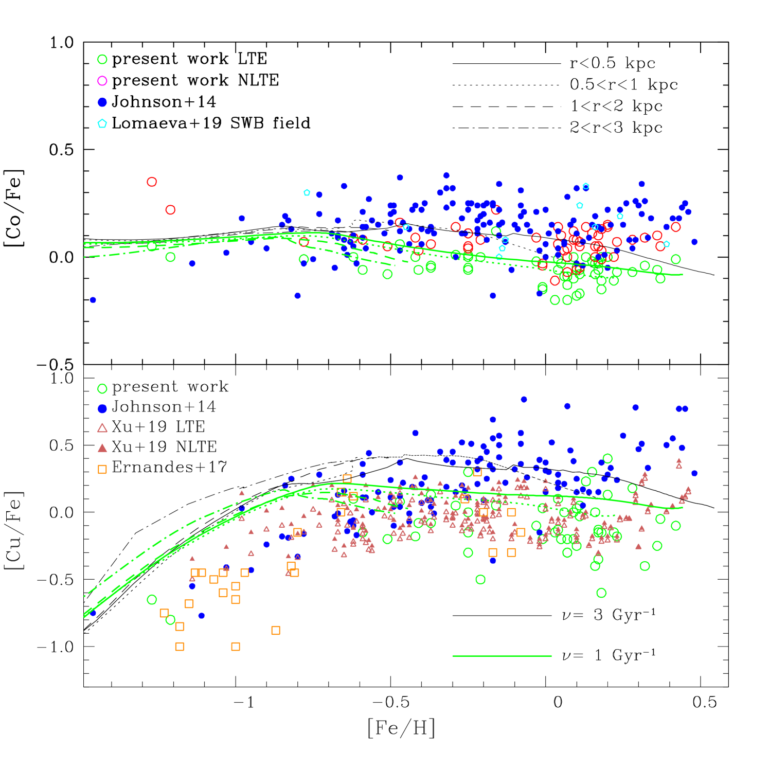
Figure 3: Upper panel: [Co/Fe] vs. [Fe/H] with the present results in LTE and corrected for NLTE, together with literature data. Lower panel: [Cu/Fe] vs. [Fe/H] with the present results and literature data. Shown are: the present results in LTE (open green circles); present results in NLTE (open magenta circles); Johnson et al. (2014) (filled blue circles); Lomaeva et al. (2019) for the SW field (open cyan circles); Xu et al. (2019) in LTE (open Indian red triangles); Xu et al. (2019) in NLTE (filled Indian red triangles); Ernandes et al. (2018) for bulge globular clusters (open dark orange squares) and chemodynamical evolution models are overplotted; specific star formation rates of 3 Gyr^-1, with SNII yields from WW95 (black lines); specific star formation rates of 1 Gyr^-1, with SNII yields from WW95 and from Kobayashi et al. (2006) for [Fe/H]$<$-4.0 (green lines). Models are for distances to the Galactic center of: r $<$ 0.5 kpc (solid lines), 0.5 $<$ r $<$ 1 kpc (dotted lines), 1 $<$ r $<$ 2 kpc (dashed lines), and 2 $<$ r $<$ 3 kpc (dash-dotted lines).

5 Discussion of results

Our main interest in the present work is to compare the behaviour of cobalt and copper. They are produced both in the alpha-rich freezeout as primary elements (Sukhbold et al. 2016) and in the weak-s process in massive stars as secondary elements. The iron-peak elements are mainly formed during explosive oxygen and silicon burning in massive supernovae (WW95). For the larger values of the neutron fraction $\eta$, the main products of silicon burning are completed. On the other hand, if the density is low and the supernova envelope expansion is fast, $\alpha$ particles will be frozen and not captured by the heavier elements (Woosley et al. 2002). This so-called $\alpha$-rich freezeout will produce ⁵⁹Co. As pointed out by S. Woosley (private communication) and Barbuy et al. (2018a), their abundances as a function of Fe can reveal the relative efficiencies of these two contributions.

In thick-disc and halo stars, Nissen et al. (2000), Cayrel et al. (2004), and Ishigaki et al. (2013), among others, derived abundances of iron-peak elements. Nissen et al. (2000) observed that Sc might be enhanced in metal-poor stars, and that Mn decreases with decreasing metallicities. Ishigaki et al. (2013) has also shown that most Fe-peak elements show solar abundance ratios as a function of metallicity, with the exception of Mn, Cu, and Zn. In particular as regards Co and Cu, Ishigaki et al. finds that Co varies in lockstep with Fe for [Fe/H]$>$-2.0, but appears enhanced for [Fe/H]$<$-2.0, as previously already found by Cayrel et al. (2004), and that Cu decreases with decreasing metallicities. Barbuy (2013, 2015) and da Silveira et al. (2018) derived Mn and Zn for the present sample of 56 UVES spectra of red giants, and confirmed that Mn decreases with decreasing metallicity and that Zn is enhanced in metal-poor stars. Ernandes et al. (2018) discussed Sc, V, Mn, Cu, and Zn in bulge globular-cluster stars from UVES spectra, with Sc and V varying in lockstep with Fe, Mn; Cu, increasing with metallicity; and Zn enhanced in metal-poor stars. We will now examine the [Co/Fe] and [Cu/Fe] versus [Fe/H] behaviour.

Before drawing conclusions, we present literature results here on Co and Cu in bulge stars. Johnson et al. (2014) derived abundances of Cr, Co, Ni, and Cu in 156 giants, and Xu et al. (2019) derived Cu abundances for 129 of these same stars, applying NLTE corrections. Recently, Lomaeva et al. (2019) derived Sc, V, Cr, Mn, Co, and Ni for bulge giants that include 33 stars in common using the same UVES data as the present sample. Schultheis et al. (2017) derived abundances of Cr, Co, Ni, and Mn from APOGEE results, which show, however, a large spread and are not considered here.

5.1 Comments on results for cobalt

Figure 3 shows that [Co/Fe] varies in lockstep with [Fe/H], and this appears in all samples. It appears therefore that the nucleosynthesis process dominating the formation of cobalt is the alpha-rich freezeout.

Figure 3 shows that the mean [Co/Fe] value differs among the different authors. The Johnson et al. (2014) and Lomaeva et al. (2019) results are in the mean 0.2 dex, more Co-rich than the present results. A main reason for the discrepancies might be the location of continuum. In order to further investigate the disagreement on the level of Co deficiency or over-enhancement, it is interesting to note the deficiency in Co relative to Fe in the Sagittarius dwarf galaxy. In Fig. 4 we compare the present results for Co in LTE and NLTE, compared with Co abundances in 158 red giants of the Sagittarius dwarf galaxy by Hasselquist et al. (2017). These authors used the H-band from APOGEE data and found that Co is deficient with respect to stars in the Milky Way. Hasselquist et al. (2017) did not consider NLTE effects; therefore, we compare our results in LTE and theirs, which leads to a difference in Co abundances of $\Delta$[Co/Fe]$\sim$0.3, reduced by 0.2 with respect to results by Johnson et al. (2014) and Lomaeva et al. (2019). Therefore, the deficiency of Co in Sagittarius relative to the present paper is not as drastic as in previous results discussed in the literature. A possible explanation of the deficiency in Co in Sagittarius, previously already suggested by McWilliam et al. (2013), is that Sagittarius was less enriched by SNe II relative to the Milky Way, which could be caused by a top-light initial mass function (IMF).

5.2 Comments on results for copper

In Fig. 3 all data agree on [Cu/Fe] versus [Fe/H] having a flat behaviour between -0.8 $<$ [Fe/H] $<$ +0.1. For [Fe/H] $<$ -0.8, copper-to-iron clearly decreases with decreasing metallicity, indicating the behaviour of a secondary element. For the metal-rich stars, our data would be compatible with a flat trend, or a slightly decreasing trend with metallicity, but this is not shown in the Johnson et al. and Xu et al. results. Finally, there is a shift in enhancements between Johnson et al. and Xu et al. Since they use the same spectra of the same stars, and the same line, this could be due to a different placement of continua. Our results fit the abundance values from Xu et al. better and we note that the NLTE corrections from Xu et al. are small.

The behaviour of [Cu/Fe] versus [Fe/H], which shows a decrease in [Cu/Fe] towards decreasing metallicities, confirms that [Cu/Fe] essentially has a secondary-element behaviour and that its production should be dominated by a weak s-process. Another characteristic, as noted by McWilliam (2016), is that [Cu/O] has much less spread than [Cu/Fe] data, indicating a production of Cu and O in the same massive stars. This is confirmed in Fig. 5, where our data are plotted in NLTE together with data from Johnson et al. (2014) and Ernandes et al. (2018), the latter corresponding to red giants in bulge globular clusters. It is clear that the spread of points is lower, confirming the suggestion by McWilliam (2016).

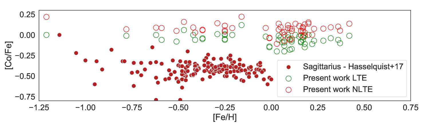
Figure 4: [Co/Fe] vs. [Fe/H]: present results in LTE and corrected for NLTE, compared with data from Hasselquist et al. (2017) for the Sagittarius dwarf galaxy. Symbols: open green circles represent present results in LTE; red circles represent present results in NLTE; filled blue dots represent Hasselquist et al. (2017).

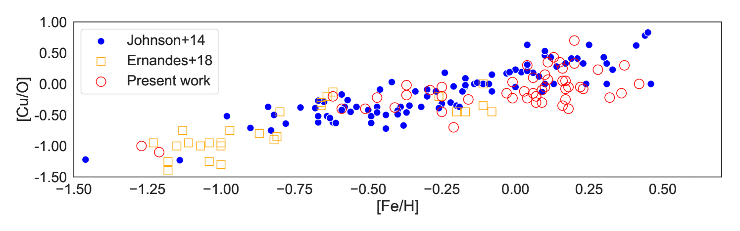
Figure 5: [Cu/O] vs. [Fe/H] for the present results in NLTE and literature data. Symbols: open magenta circles represent present results in NLTE; filled blue dots represent Jonhson et al. (2014); open orange squares represent Ernandes et al. (2018).

6 Conclusions

We derived the abundances of the iron-peak elements Co and Cu in 56 red giants of the Galactic bulge, for which we have previously derived abundances of C, N, O, Na, Mg, Al, Mn, Zn, and heavy elements. The abundances of C, N, O, Na, Mg, Al, Mn, Co, Cu, and Zn are gathered in Table 12.

Cobalt and copper are in the so-called upper iron-group. The upper iron-group elements Co, Ni, Cu, Zn, Ga, and Ge with 27 $\leq$ Z $\leq$ 32, or 57$\leq$A$\leq$66 (up to ⁶⁶Zn, but excluding ^67,68Zn, ⁶⁹Ga,^70,71Ge) are mainly produced in two processes, namely, a) neutron capture on iron-group nuclei during He burning and later burning stages, also called weak s-component, and b) the $\alpha$-rich freezeout in the deepest layers (Woosley et al. 1973), also discussed in WW95, Limongi et al. (2003), Woosley et al. (2002), and Sukhbold et al. (2016). The nucleosynthesis yields from the weak s-component show a characteristic secondary behaviour.

In this work we analysed a sample of high-quality spectroscopic data for 56 Galactic bulge red giants. The present results show [Co/Fe] $\sim$ constant $\sim$ 0.0, indicating cobalt mainly produced from the $\alpha$-rich freezeout. Copper instead shows a secondary element behaviour, with [Cu/Fe] decreasing with decreasing metallicity, indicating its production to be dominated by the weak s-process. The yields of Co and Cu considered in the models appear to include these two mechanisms in the right proportions, and the chemodynamical models reproduce their behaviour well.

Table 6: Comparison of stellar parameters and Co and Cu abundances of the present work with Johnson et al. (2014) and Lomaeva et al. (2019).

Star	OGLE	Teff	logg	[Fe/H]	vt	[Co/Fe]LTE	[Co/Fe]NLTE	[Cu/Fe]	Teff	logg	[Fe/H]	[Co/Fe]	[Cu/Fe]
			Present work								Johnson et al. 2014
B3-b2	262018C7	4500	2.0	0.18	1.5	-0.11	0.03	-0.15	4700	2.75	0.08	0.15	0.46
B3-b4	215681C6	4500	2.1	0.17	1.7	-0.03	0.10	-0.13	4800	2.75	0.31	0.20	0.51
B3-b5	286252C7	4600	2.0	0.11	1.5	-0.06	0.07	0.05	4700	3.10	0.43	0.18	0.77
B3-b7	282804C7	4400	1.9	0.20	1.3	0.00	0.14	0.13	4575	2.50	0.10	0.11	0.25
B3-b8	240083C6	4400	1.8	-0.62	1.4	0.00	0.09	0.10	4425	1.65	-0.58	0.04	—
B3-f1	129499C4	4500	1.9	0.04	1.6	-0.06	0.06	-0.13	4900	2.75	0.13	0.32	—
B3-f8	193190C5	4800	1.9	0.20	1.5	0.00	0.15	0.40	4675	2.75	0.24	0.22	—
Star	OGLE	Teff	logg	[Fe/H]	vt	[Co/Fe]LTE	[Co/Fe]NLTE	[Cu/Fe]	Teff	logg	[Fe/H]	vt	[Co/Fe]LTE
			Present work								Lomaeva et al. 2019
B3-b1	132160C4	4300	1.7	-0.78	1.5	-0.01	0.07	—	4414	1.35	-0.89	1.41	0.04
B3-b5	286252C7	4600	2.0	0.11	1.5	-0.06	0.07	0.05	4425	2.70	0.25	1.43	-0.25
B3-b7	282804C7	4400	1.9	0.20	1.3	0.00	0.14	0.13	4303	2.36	0.08	1.58	-0.08
B3-b8	240083C6	4400	1.8	-0.62	1.4	0.00	0.09	0.10	4287	1.79	-0.67	1.46	0.67
B3-f1	129499C4	4500	1.9	0.04	1.6	-0.06	0.06	-0.13	4485	2.25	-0.15	1.88	0.15
B3-f2	259922C7	4600	1.9	-0.25	1.8	+0.01	0.11	0.30	4207	1.64	-0.66	1.74	0.66
B3-f3	95424C3	4400	1.9	0.06	1.7	-0.09	0.03	0.00	4637	2.96	0.24	1.89	-0.24
B3-f4	208959C6	4400	2.1	0.09	1.5	-0.10	0.08	-0.20	4319	2.60	-0.12	1.50	0.12
B3-f7	279577C7	4800	2.1	0.16	1.7	-0.08	0.05	0.00	4517	2.93	0.17	1.55	-0.17
B3-f8	193190C5	4800	1.9	0.20	1.5	0.00	0.15	0.40	4436	2.88	0.24	1.54	-0.24
BW-b1									4042	2.39	0.46	1.43	-0.46
BW-b2	214192	4300	1.9	0.22	1.5	-0.11	0.00	-0.15	4367	2.39	0.18	1.68	-0.18
BW-b5	82760	4000	1.6	0.17	1.2	-0.02	0.05	-0.35	3939	1.68	0.25	1.31	-0.25
BW-b6	392931	4200	1.7	-0.25	1.3	-0.06	0.04	-0.30	4262	1.98	-0.32	1.44	0.32
BW-b8									4424	2.54	0.30	1.52	-0.30
BW-f1	433669	4400	1.8	0.32	1.6	-0.04	0.09	-0.40	4359	2.51	0.28	1.93	-0.28
BW-f5	240260	4800	1.9	-0.59	1.3	-0.06	0.08	-0.15	4818	2.89	-0.51	1.29	0.51
BW-f6	392918	4100	1.7	-0.21	1.5	0.00	0.08	-0.50	4117	1.43	-0.43	1.69	0.43
B6-b1	29280c3	4400	1.8	0.07	1.6	-0.20	-0.07	-0.20	4372	2.59	0.25	1.57	-0.25
B6-b3	31220c2	4700	2.0	0.10	1.6	-0.05	0.08	0.03	4468	2.48	0.05	1.67	-0.05
B6-b4	60208c7	4400	1.9	-0.41	1.7	-0.06	0.03	-0.08	4215	1.38	-0.62	1.68	0.62
B6-b5	31090c2	4600	1.9	-0.37	1.3	-0.05	0.06	0.13	4340	2.02	-0.48	1.34	0.20
B6-b6	77743c7	4600	1.9	0.11	1.8	-0.08	0.05	-0.03	4396	2.37	0.19	1.77	0.23
B6-b8	108051c7	4100	1.6	0.03	1.3	-0.20	-0.11	-0.15	4021	1.90	0.06	1.45	0.06
B6-f1	23017c3	4200	1.6	-0.01	1.5	-0.14	-0.03	-0.20	4149	2.01	0.10	1.65	0.10
B6-f3	21259c2	4800	1.9	-0.29	1.3	+0.01	0.14	0.05	4565	2.60	-0.35	1.28	0.17
B6-f5	33058c2	4500	1.8	-0.37	1.4	-0.04	0.06	-0.08	4345	2.32	-0.33	1.41	0.29
B6-f7	100047c6	4300	1.7	-0.42	1.6	0.00	0.09	-0.18	4250	2.10	-0.31	1.65	0.25
B6-f8	11653c3	4900	1.8	0.04	1.6	-0.01	0.14	0.10	4470	2.78	0.13	1.30	0.13
BL-1	1458c3	4500	2.1	-0.16	1.5	+0.12	0.22	0.05	4370	2.19	-0.19	1.50	0.10
BL-3	1859c2	4500	2.3	-0.03	1.4	-0.02	0.09	-0.10	4555	2.48	-0.09	1.53	0.16
BL-4	3328c6	4700	2.0	0.13	1.5	+0.00	0.14	0.23	4476	2.94	0.27	1.41	0.19
BL-5	1932c2	4500	2.1	0.16	1.6	-0.08	0.05	0.00	4425	2.65	0.28	1.68	0.22
BL-7	6336c7	4700	2.4	-0.47	1.4	+0.06	0.16	0.08	4776	2.52	-0.5	1.53	0.19

Appendix A Atomic data

The hyperfine structure constants of Co I and Cu I lines employed in this work are given in Table 7. In Tables 8, 9, and 10, the lines of Co I in terms of their HFS components, and corresponding oscillator strengths, are listed.

Table 7: Atomic constants for CoI and CuI used to compute hyperfine structure: A and B constants from Pickering (1996) for CoI. For CuI, the A and B constants are from Kurúcz (1993) and Biehl (1976), and they are reported in Ernandes et al. (2018).

Species	$\lambda$ (Å)	-Lower level	-J	-A(mK)	-A(MHz)	-B(mK)	-B(MHz)	-Upper level	-J	-A(mK)	-A(MHz)	-B(mK)	-B(MHz)
59CoI	4749.612	(4F)4sp z6D	9/2	28.05	840.9180	0.08	2.3983	(5F)s5s e6F	11/2	31.45	942.8475	0.07	2.0985
59CoI	5212.691	(4F)4sp z4F	9/2	27.02	810.0394	0.08	2.3983	(5F)s5s f4F	11/2	35.92	1076.8546	0.07	2.0985
59CoI	5280.629	(4F)4sp z4G	9/2	17.25	517.1420	0.09	2.6981	(5F)s5s f4F	7/2	28.25	846.9138	0.07	2.0985
59CoI	5301.047	d7s4 a44P	5/2	5.90	176.8776	0.20	5.9959	(3F)4p y4D	5/2	15.50	464.6784	0.20	5.9959
59CoI	5342.708	(3F)4p y4G	11/2	10.0	299.7925	0.20	5.9959	(3F)4d e4H	13/2	7.60	227.8423	0.20	5.9959
59CoI	5454.572	(3F)4p y4F	9/2	9.90	296.7946	0.10	2.9979	(3F)4d g4F	9/2	9.18	275.2095	0.08	2.3983
59CoI	5647.234	(3P)4s a2P	3/2	11.20	335.7676	0.20	5.9959	(3F)4p y3D	5/2	16.40	491.6597	0.10	2.9979
59CoI	6117.000	d4s2 a4P	1/2	-23.60	-707.5103	0.20	5.9959	3(4F)4sp z4D	1/2	27.50	824.4294	0.10	2.9979
59CoI	6188.996	d7s2 a4P	5/2	5.90	176.8776	0.08	2.3983	(5F)4sp z4D	5/2	23.22	696.1182	0.09	2.6981
63CuI	5105.537	4p 2P [case e]	1.5	6.5	194.865	-0.96	-28.78	4s2 2D [case b]	2.5	24.97	748.582	6.20	185.871
	5218.197	4p 2P [case e]	1.5	6.5	194.865	-0.96	-28.78	4d 2D [—]	2.5	0.0*	0.0*	0.0*	0.0*
65CuI	5105.537	4p 2P [case e]	1.5	6.96	208.66	-0.86	-25.78	4s2 2D [case b]	2.5	26.79	803.14	5.81	174.18
	5218.197	4p 2P [case e]	1.5	6.96	208.66	-0.86	-25.78	4d 2D [—]	2.5	0.0*	0.0*	0.0*	0.0*

Table 8: Hyperfine structure for Co I lines.

4749.612Å; $\chi$= 3.053 eV				5212.691Å; $\chi$= 3.514 eV				5280.629Å; $\chi$= 3.629 eV
log gf(total) = $-$0.321				log gf(total) = $-$0.110				log gf(total) = $-$0.030
$\lambda$ (Å)	log gf	iso		$\lambda$ (Å)	log gf	iso		$\lambda$ (Å)	log gf	iso
4746.669	-1.7470	59		5212.691	-1.5360	59		5280.629	-1.8362	59
4749.651	-1.7470	59		5212.771	-1.5360	59		5280.660	-1.8362	59
4749.664	-2.1985	59		5212.786	-1.9875	59		5280.652	-1.7692	59
4749.643	-1.6287	59		5212.757	-1.4177	59		5280.637	-2.4682	59
4749.683	-3.1985	59		5212.808	-2.9875	59		5280.662	-1.5729	59
4749.662	-1.9877	59		5212.779	-1.7767	59		5280.646	-1.5729	59
4749.633	-1.5106	59		5212.740	-1.2996	59		5280.623	-2.3133	59
4749.687	-2.9925	59		5212.808	-2.7815	59		5280.661	-1.3688	59
4749.659	-1.8921	59		5212.770	-1.6811	59		5280.637	-1.4682	59
4749.623	-1.3992	59		5212.721	-1.1882	59		5280.605	-2.3133	59
4749.690	-2.9645	59		5212.806	-2.7535	59		5280.656	-1.1994	59
4749.655	-1.8561	59		5212.757	-1.6451	59		5280.625	-1.4212	59
4749.612	-1.2954	59		5212.699	-1.0844	59		5280.585	-2.4102	59
4749.693	-3.0436	59		5212.801	-2.8326	59		5280.649	-1.0532	59
4749.650	-1.8717	59		5212.743	-1.6607	59		5280.609	-1.4268	59
4749.601	-1.1989	59		5212.674	-0.9879	59		5280.563	-2.6143	59
4749.694	-3.2355	59		5212.794	-3.0245	59		5280.638	-0.9241	59
4749.645	-1.9539	59		5212.726	-1.7429	59		5280.591	-1.5004	59
4749.588	-1.1088	59		5212.648	-0.8978	59		5280.536	-3.0123	59
4749.695	-3.6245	59		5212.785	-3.4135	59		5280.625	-0.8082	59
4749.639	-2.1722	59		5212.707	-1.9612	59		5280.570	-1.7112	59
4749.575	-1.0245	59		5212.619	-0.8135	59		5280.608	-0.7026	59

Table 9: Hyperfine structure for Co I lines.

5301.047Å; $\chi$= 1.710 eV				5342.708Å; $\chi$= 4.021 eV				5454.572Å; $\chi$= 4.072 eV
log gf(total) = $-$2.000				log gf(total) = 0.690				log gf(total) = +0.238
$\lambda$ (Å)	log gf	iso		$\lambda$ (Å)	log gf	iso		$\lambda$ (Å)	log gf	iso
5301.077	-3.6513	59		5342.700	-0.5933	59		5454.568	-1.4018	59
5301.068	-3.3960	59		5342.708	-1.3181	59		5454.562	-1.5981	59
5301.081	-3.3960	59		5342.700	-0.5100	59		5454.574	-1.5981	59
5301.072	-5.3045	59		5342.720	-2.5312	59		5454.568	-1.3877	59
5301.059	-3.1973	59		5342.711	-1.0998	59		5454.560	-1.3774	59
5301.077	-3.1973	59		5342.701	-0.4239	59		5454.577	-1.3774	59
5301.064	-4.0615	59		5342.726	-2.2971	59		5454.569	-1.2504	59
5301.046	-3.1328	59		5342.715	-1.0058	59		5454.558	-1.2738	59
5301.070	-3.1328	59		5342.702	-0.3396	59		5454.581	-1.2738	59
5301.053	-3.3442	59		5342.732	-2.2513	59		5454.570	-1.0827	59
5301.031	-3.1639	59		5342.719	-0.9739	59		5454.556	-1.2313	59
5301.061	-3.1639	59		5342.704	-0.2585	59		5454.584	-1.2313	59
5301.040	-2.9376	59		5342.739	-2.3183	59		5454.571	-0.9143	59
5301.013	-3.3454	59		5342.724	-0.9941	59		5454.554	-1.2416	59
5301.049	-3.3454	59		5342.707	-0.1810	59		5454.588	-1.2416	59
5301.023	-2.6465	59		5342.747	-2.5012	59		5454.572	-0.7549	59
				5342.729	-1.0809	59		5454.553	-1.3194	59
				5342.709	-0.1073	59		5454.593	-1.3194	59
				5342.755	-2.8833	59		5454.573	-0.6070	59
				5342.735	-1.3036	59		5454.552	-1.5340	59
				5342.713	-0.0370	59		5454.597	-1.5340	59
								5454.575	-0.4706	59

Table 10: Hyperfine structure for Co I lines.

5647.234Å; $\chi$= 2.280 eV				6117.000Å; $\chi$= 1.785 eV				6188.996Å; $\chi$= 1.710 eV
log gf(total) = $-$1.560				log gf(total) = $-$2.490				log gf(total) = $-$2.450
$\lambda$ (Å)	log gf	iso		$\lambda$ (Å)	log gf	iso		$\lambda$ (Å)	log gf	iso
5105.562	$-$2.8856	59		5218.195	$-$1.2041	63		5218.195	$-$1.2041	59
5647.269	-2.7641	59		6117.043	-3.4511	59		6189.071	-4.1013	59
5647.258	-2.7641	59		6117.002	-2.9740	59		6189.053	-3.8460	59
5647.243	-3.0652	59		6117.008	-2.9740	59		6189.075	-3.8460	59
5647.269	-2.9402	59		6116.967	-3.1201	59		6189.058	-5.7545	59
5647.253	-2.6003	59						6189.031	-3.6473	59
5647.232	-2.6258	59						6189.064	-3.6473	59
5647.268	-3.1901	59						6189.038	-4.5115	59
5647.247	-2.5924	59						6189.002	-3.5828	59
5647.220	-2.3425	59						6189.046	-3.5828	59
5647.265	-3.6180	59						6189.011	-3.7942	59
5647.238	-2.7527	59						6188.967	-3.6139	59
5647.207	-2.1273	59						6189.022	-3.6139	59
								6188.978	-3.3876	59
								6188.924	-3.7954	59
								6188.991	-3.7954	59
								6188.938	-3.0965	59

Appendix B NLTE corrections to cobalt abundances

The NLTE corrections to the derived LTE abundances of Co, derived from calculations made available online by Bergemann et al. (2010) (see text), are given in Table 11.

Table 11: NLTE corrections to the derived LTE abundances of Co.

Star	[Co/Fe]	[Co/Fe]	[Co/Fe]	[Co/Fe]	[Co/Fe]	[Co/Fe]	[Co/Fe]	[Co/Fe]
	5212.691 Å	5280.629 Å	5301.047 Å	5342.708 Å	5454.572 Å	5647.234 Å	6117.000 Å	6188.996 Å
B6-b1	0.117	0.169	0.341	0.000	0.000	0.219	0.088	0.081
B6-b2	0.097	0.146	0.312	0.000	0.000	0.186	0.074	0.066
B6-b3	0.124	0.185	0.320	0.000	0.000	0.216	0.094	0.106
B6-b4	0.105	0.119	0.274	0.000	0.000	0.138	0.038	0.036
B6-b5	0.123	0.158	0.255	0.000	0.000	0.169	0.072	0.074
B6-b6	0.122	0.181	0.333	0.000	0.000	0.220	0.088	0.097
B6-b8	0.088	0.129	0.266	0.000	0.000	0.157	0.052	0.047
B6-f1	0.095	0.137	0.302	0.000	0.000	0.182	0.068	0.061
B6-f2	0.158	0.199	0.245	0.000	0.000	0.192	0.123	0.115
B6-f3	0.147	0.202	0.255	0.000	0.000	0.204	0.126	0.128
B6-f5	0.116	0.145	0.285	0.000	0.000	0.165	0.060	0.059
B6-f7	0.101	0.116	0.302	0.000	0.000	0.139	0.036	0.031
B6-f8	0.139	0.216	0.283	0.000	0.000	0.224	0.145	0.163
BW-b2	0.111	0.167	0.287	0.000	0.000	0.191	0.075	0.067
BW-b4	0.111	0.186	0.342	0.000	0.000	0.214	0.102	0.091
BW-b5	0.078	0.123	0.210	0.000	0.000	0.121	0.012	0.030
BW-b6	0.101	0.122	0.320	0.000	0.000	0.164	0.052	0.039
BW-b7	0.105	0.177	0.322	0.000	0.000	0.196	0.087	0.077
BW-f1	0.131	0.212	0.314	0.000	0.000	0.213	0.098	0.091
BW-f4	0.305	0.270	0.343	0.000	0.000	0.305	0.285	0.244
BW-f5	0.188	0.220	0.243	0.000	0.000	0.212	0.155	0.140
BW-f6	0.091	0.116	0.268	0.000	0.000	0.135	0.035	0.028
BW-f7	0.118	0.165	0.329	0.000	0.000	0.216	0.088	0.079
BW-f8	0.407	0.347	0.468	0.000	0.000	0.412	0.415	0.363
BL-1	0.105	0.132	0.301	0.000	0.000	0.173	0.051	0.052
BL-3	0.106	0.133	0.307	0.000	0.000	0.190	0.057	0.049
BL-4	0.128	0.194	0.329	0.000	0.000	0.227	0.100	0.109
BL-5	0.122	0.174	0.327	0.000	0.000	0.222	0.092	0.081
BL-7	0.131	0.160	0.197	0.000	0.000	0.154	0.074	0.070
B3-b1	0.122	0.119	0.216	0.000	0.000	0.113	0.039	0.022
B3-b2	0.131	0.193	0.348	0.000	0.000	0.233	0.106	0.092
B3-b3	0.124	0.177	0.329	0.000	0.000	0.218	0.097	0.080
B3-b4	0.122	0.171	0.322	0.000	0.000	0.219	0.090	0.081
B3-b5	0.125	0.185	0.340	0.000	0.000	0.229	0.091	0.092
B3-b7	0.131	0.200	0.348	0.000	0.000	0.226	0.105	0.087
B3-b8	0.120	0.130	0.244	0.000	0.000	0.135	0.046	0.034
B3-f1	0.115	0.168	0.339	0.000	0.000	0.216	0.080	0.079
B3-f2	0.112	0.149	0.260	0.000	0.000	0.162	0.065	0.075
B3-f3	0.112	0.154	0.324	0.000	0.000	0.207	0.076	0.071
B3-f4	0.108	0.148	0.304	0.000	0.000	0.200	0.074	0.063
B3-f5	0.089	0.120	0.235	0.000	0.000	0.155	0.045	0.045
B3-f7	0.124	0.189	0.301	0.000	0.000	0.213	0.102	0.118
B3-f8	0.141	0.222	0.342	0.000	0.000	0.248	0.130	0.141
BWc-1	0.112	0.158	0.317	0.000	0.000	0.211	0.077	0.069
BWc-2	0.132	0.191	0.340	0.000	0.000	0.232	0.107	0.087
BWc-3	0.146	0.221	0.355	0.000	0.000	0.239	0.117	0.095
BWc-4	0.124	0.186	0.270	0.000	0.000	0.202	0.106	0.120
BWc-5	0.155	0.247	0.328	0.000	0.000	0.231	0.114	0.099
BWc-6	0.125	0.174	0.231	0.000	0.000	0.178	0.090	0.095
BWc-7	0.114	0.145	0.282	0.000	0.000	0.173	0.062	0.060
BWc-8	0.159	0.244	0.347	0.000	0.000	0.243	0.125	0.104
BWc-9	0.125	0.178	0.331	0.000	0.000	0.226	0.093	0.084
BWc-10	0.122	0.182	0.290	0.000	0.000	0.206	0.097	0.107
BWc-11	0.139	0.207	0.365	0.000	0.000	0.244	0.117	0.097
BWc-12	0.141	0.209	0.353	0.000	0.000	0.240	0.116	0.097
BWc-13	0.162	0.262	0.373	0.000	0.000	0.252	0.129	0.108

Appendix C Fits of studied lines to the spectra of the Sun, Arcturus, and $\mu$ Leo

The lines of Cu I and Co I employed to derive abundances in the present work were first fitted to the spectra of the Sun, Arcturus, and $\mu$ Leo, as shown in Figs. 6 and 7. Details on the adopted parameters are given in Sect. 3.

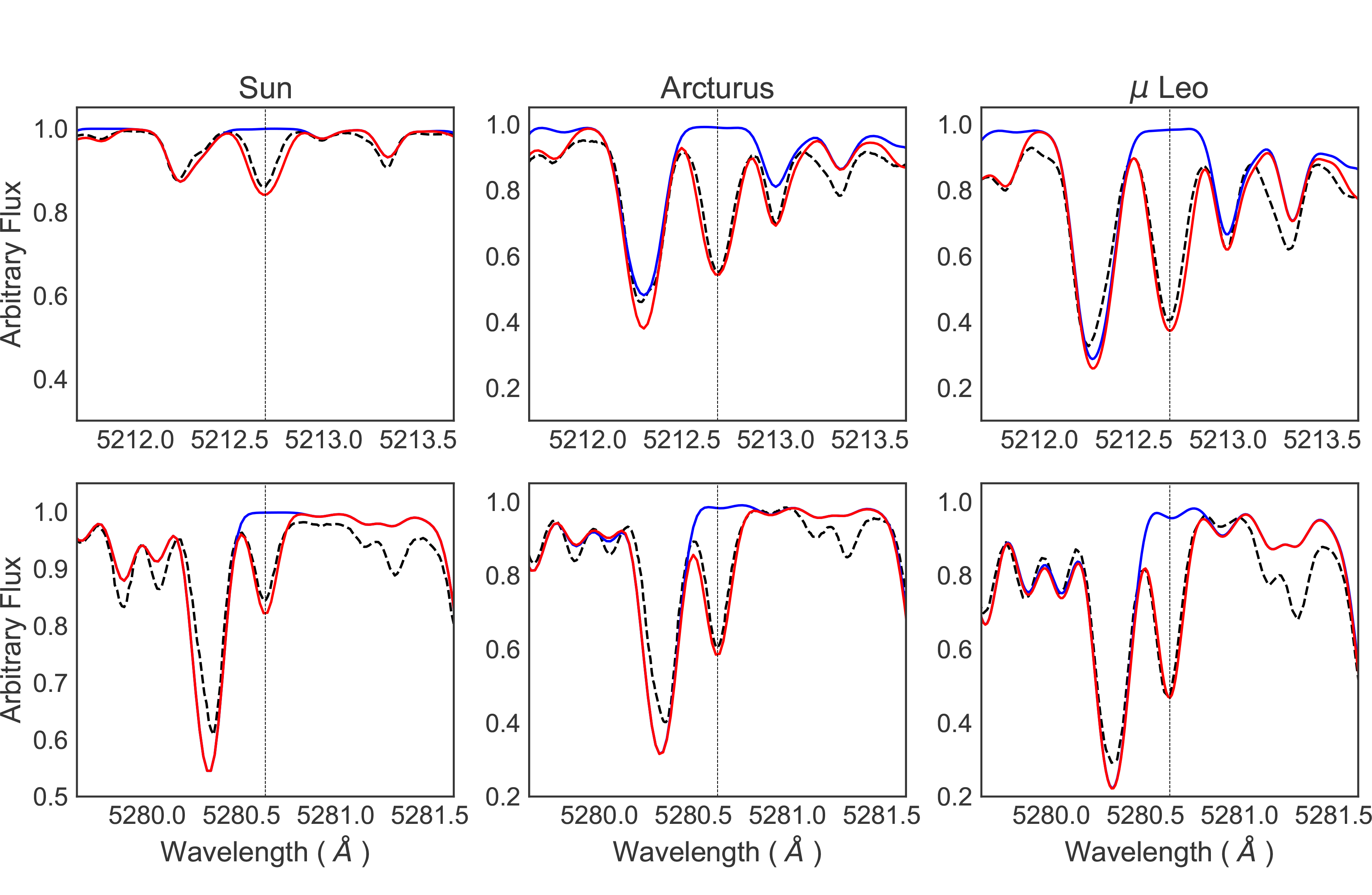
(a) Co I 5212.537, 5280.629 Å

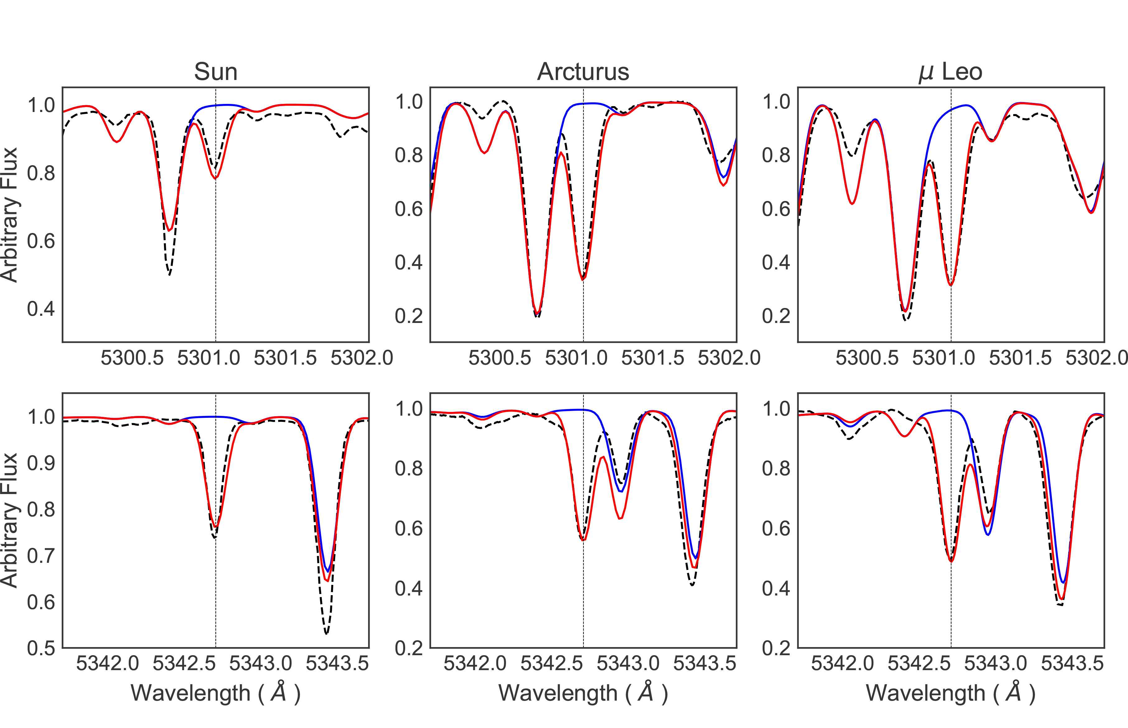
(b) Co I 5301.039, 5342.695 Å

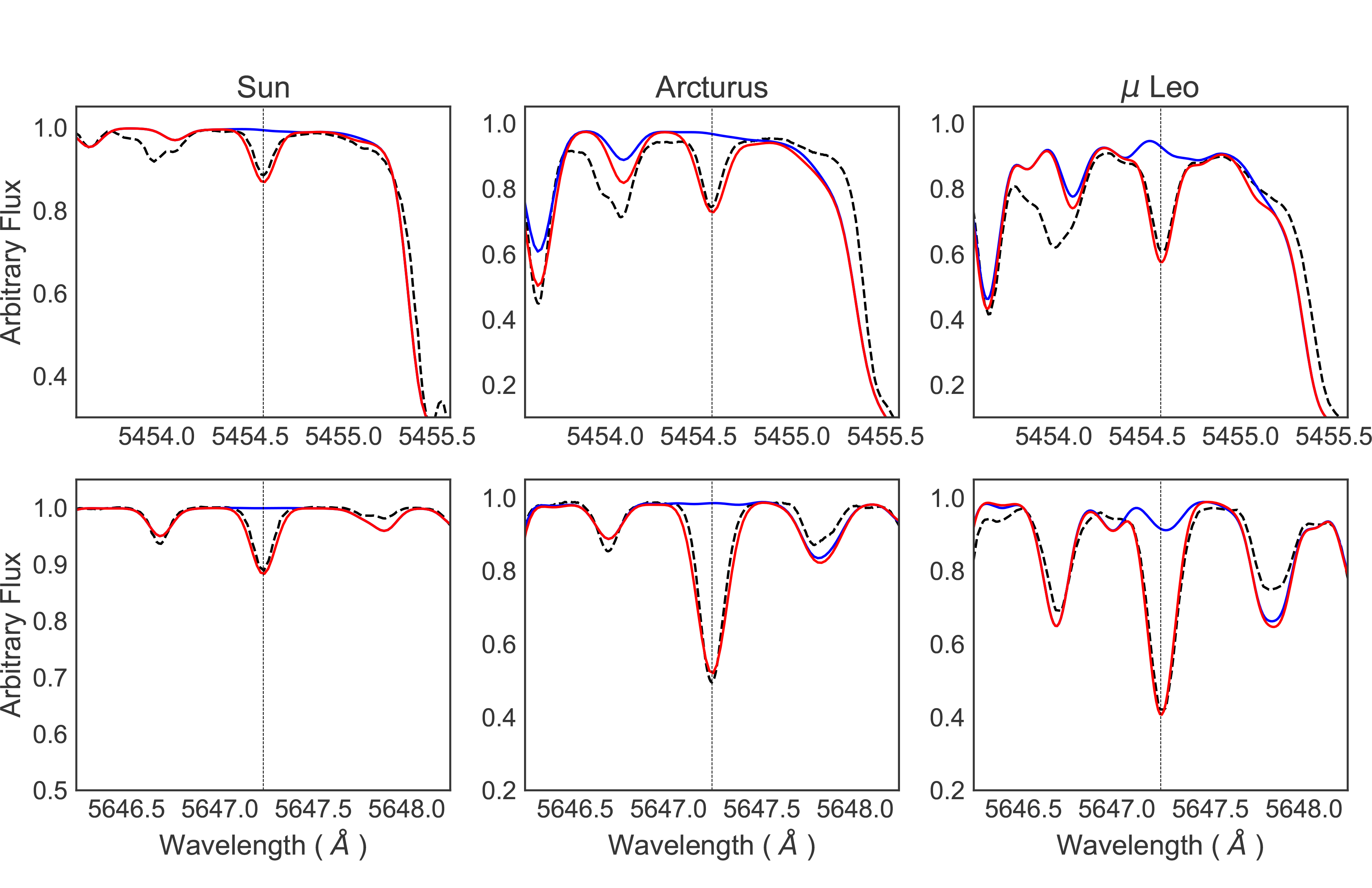
(c) Co I 5454.572, 5647.234 Å

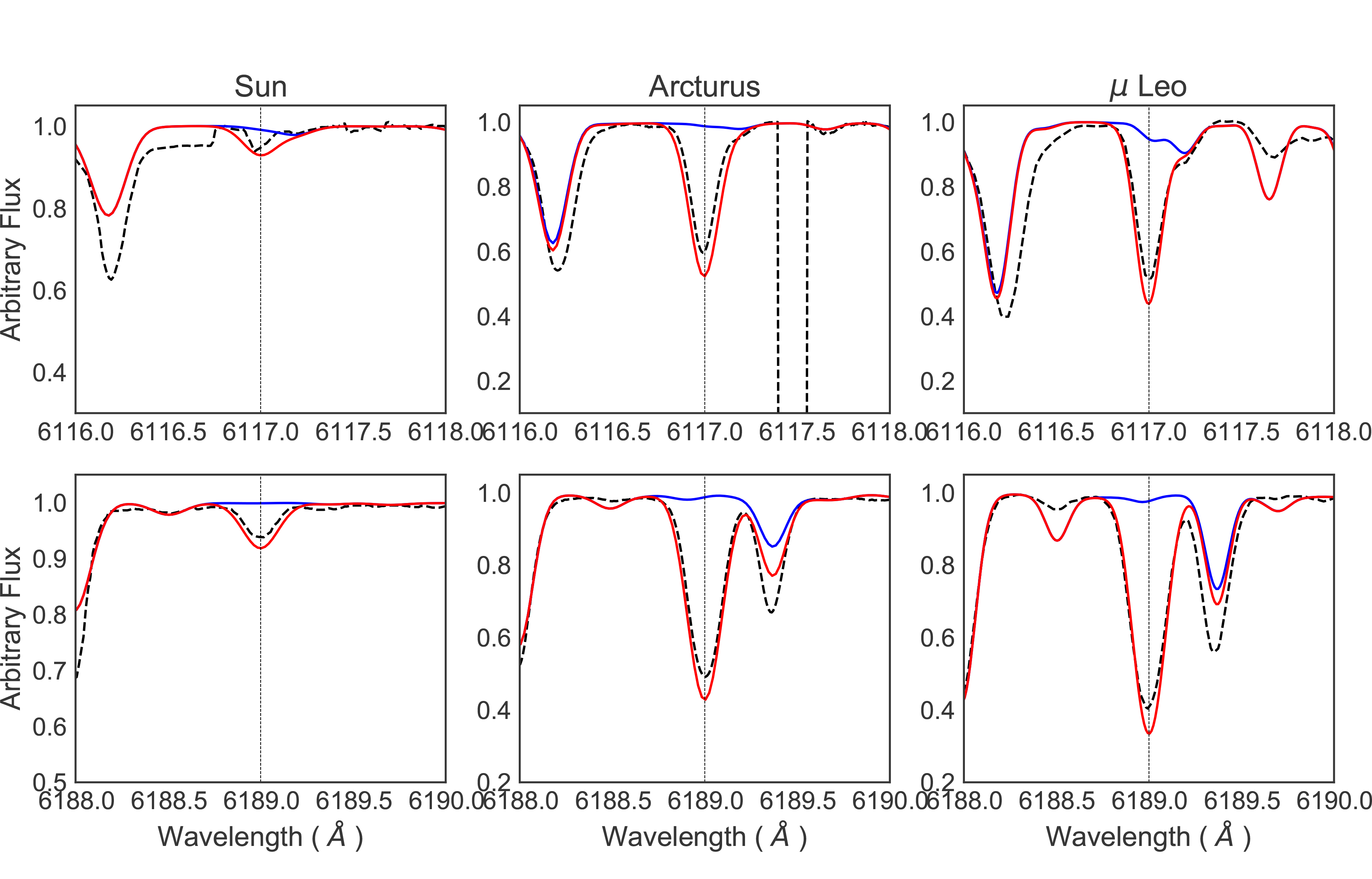
(d) Co I 6117.0, 6188.996 Å

Figure 6: Cobalt lines as fitted to the Sun, Arcturus, and $\mu$ Leo.

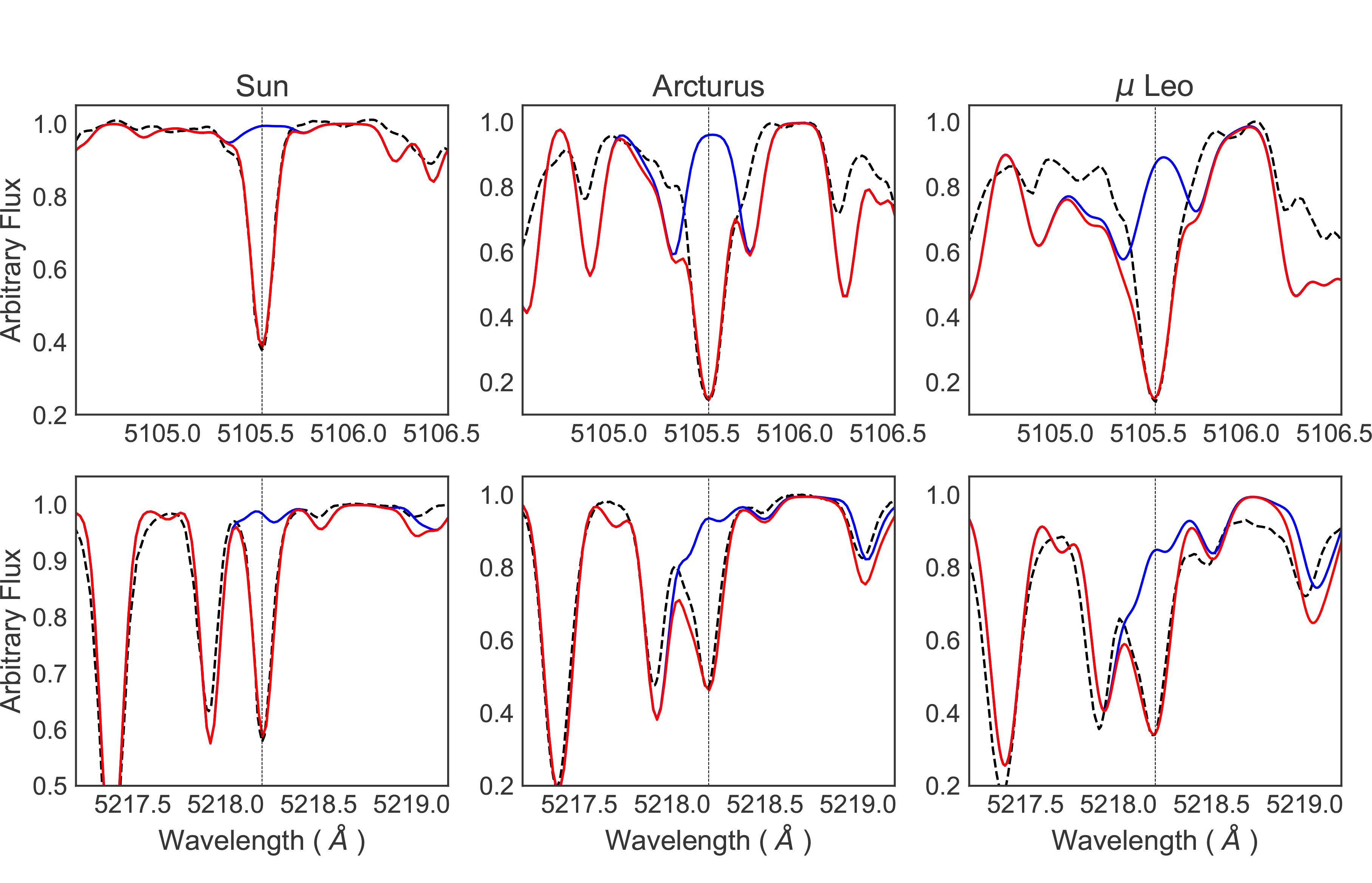
Figure 7: Copper lines Cu I 5105.537 and 5218.197 Å, as fitted to the Sun, Arcturus, and $\mu$ Leo.

Appendix D Abundances of C, N, O, Na, Mg, Al, Mn, Co, and Cu for the 56 sampled red giants

In Table 12, the metallicity from Zoccali et al. (2006), Lecureur et al. (2007), and Hill et al. (2011) for the 56 sample red giants is reported in column 2 . The abundances of C, N, O, Na, Mg, Al, Mn, Co, Cu, and Zn from the following sources are reported: CNO abundances revised in Friaça & Barbuy (2017); Na, Mg, and Al from Lecureur et al. (2007); Mn from Barbuy et al. (2013); Zn from Barbuy et al. (2015) and da Silveira et al. (2018); and the present results on Co (LTE and NLTE-corrected) and Cu.

Table 12: Metallicity [Fe/H] and abundances of C, N, O, Na, Mg, Al, Mn, Co, Cu for the 56 sample red giants.

Star	[Fe/H]	[C/Fe]	[N/Fe]	[O/Fe]	[Na/Fe]	[Mg/Fe]	[Al/Fe]	[Mn/Fe]	[Cu/Fe]	[Co/Fe]LTE	[Co/Fe]NLTE	[Zn/Fe]
B6-b1	0.07	-0.15	0.50	0.00	0.57	0.21	0.59	0.06	-0.20	-0.20	-0.07	-0.20
B6-b2	-0.01	-0.05	0.35	0.00	—	—	—	-0.03	0.03	-0.15	-0.04	-0.15
B6-b3	0.10	-0.25	0.50	-0.12	0.45	0.21	0.43	0.00	0.03	-0.05	0.08	-0.27
B6-b4	-0.41	-0.15	0.15	0.30	0.15	0.41	0.31	-0.20	-0.08	-0.06	0.03	0.00
B6-b5	-0.37	-0.10	0.30	0.15	0.32	0.42	0.58	-0.04	0.13	-0.05	0.06	0.10
B6-b6	0.11	-0.15	0.50	-0.10	0.68	0.32	0.67	0.00	-0.03	-0.08	0.05	-0.40
B6-b8	0.03	0.00	0.10	-0.03	0.46	0.31	0.50	-0.03	-0.15	-0.20	-0.11	-0.08
B6-f1	-0.01	0.05	0.20	0.03	0.20	0.24	0.41	0.02	-0.20	-0.14	-0.03	-0.30
B6-f2	-0.51	0.00	0.20	0.20	0.22	0.44	0.57	-0.08	-0.20	-0.08	0.05	0.05
B6-f3	-0.29	-0.05	0.30	0.15	0.31	0.43	0.53	0.00	0.05	0.01	0.14	0.10
B6-f5	-0.37	0.05	0.00	0.10	0.23	0.41	0.74	-0.08	-0.08	-0.04	0.06	0.10
B6-f7	-0.42	0.00	0.30	—	0.22	0.54	0.68	0.00	-0.18	0.00	0.09	-0.15
B6-f8	0.04	-0.10	0.30	-0.20	0.50	0.27	0.72	0.00	0.10	-0.01	0.14	-0.60
BW-b2	0.22	-0.10	0.20	-0.10	0.01	0.40	0.26	0.00	-0.15	-0.11	0.00	-0.15
BW-b4	0.07	-0.10	0.00	-0.10	—	—	—	0.00	-0.30	-0.13	0.00	0.00
BW-b5	0.17	0.00	0.05	-0.10	0.37	0.19	0.49	0.00	-0.35	-0.02	0.05	-0.30
BW-b6	-0.25	0.00	0.65	0.15	0.22	0.59	0.55	0.00	-0.30	-0.06	0.04	0.00
BW-b7	0.10	-0.25	0.10	-0.20	—	—	—	0.00	-0.25	-0.18	-0.06	-0.30
BW-f1	0.32	-0.20	0.45	-0.18	0.93	0.46	0.49	0.00	-0.40	-0.04	0.09	-0.35
BW-f4	-1.21	0.30	0.30	0.30	-0.06	0.42	0.86	-0.72	-0.80	0.00	0.22	0.30
BW-f5	-0.59	0.10	0.40	0.25	0.23	0.45	0.50	0.00	-0.15	-0.06	0.08	0.15
BW-f6	-0.21	0.08	0.40	0.20	-0.08	0.61	0.25	0.00	-0.50	0.00	0.08	0.15
BW-f7	0.11	-0.20	0.70	-0.25	0.36	0.29	0.26	0.00	—	-0.17	-0.05	-0.20
BW-f8	-1.27	0.00	0.20	0.35	9.99	0.56	9.99	-0.60	-0.65	0.05	0.35	0.30
BL-1	-0.16	0.15	0.40	0.30	0.17	0.32	0.44	-0.01	0.05	0.12	0.22	0.05
BL-3	-0.03	0.07	0.00	0.05	0.03	0.35	0.40	-0.02	-0.10	-0.02	0.09	0.10
BL-4	0.13	-0.10	0.20	-0.20	0.70	0.39	0.78	0.00	0.23	0.00	0.14	-0.30
BL-5	0.16	0.00	0.40	-0.05	0.51	0.32	0.58	0.00	0.00	-0.08	0.05	-0.27
BL-7	-0.47	0.00	0.30	0.30	0.06	0.46	0.36	-0.30	0.08	0.06	0.16	0.30
B3-b1	-0.78	0.00	0.60	0.35	0.04	0.53	0.40	-0.35	—	-0.01	0.07	0.30
B3-b2	0.18	—	0.20	-0.10	0.27	0.35	0.19	0.00	-0.15	-0.11	0.03	-0.10
B3-b3	0.18	-0.10	0.00	-0.20	0.46	0.37	0.37	0.00	—	0.00	0.13	—
B3-b4	0.17	-0.15	0.40	-0.05	0.49	0.50	0.27	0.00	-0.13	-0.03	0.10	0.00
B3-b5	0.11	-0.20	0.00	-0.30	0.56	0.32	0.59	0.00	0.05	-0.06	0.07	0.00
B3-b7	0.20	-0.15	0.25	-0.20	0.34	0.12	0.39	0.00	0.13	0.00	0.14	-0.50
B3-b8	-0.62	-0.15	0.15	0.30	-0.02	0.47	0.34	-0.10	0.10	0.00	0.09	0.30
B3-f1	0.04	0.00	0.40	0.10	0.45	0.35	0.52	0.00	-0.13	-0.06	0.06	0.00
B3-f2	-0.25	—	—	—	0.53	0.55	0.66	0.00	0.30	0.01	0.11	0.00
B3-f3	0.06	0.00	0.00	-0.10	0.34	0.54	0.25	0.00	0.00	-0.09	0.03	0.00
B3-f4	0.09	0.00	0.10	0.10	9.99	0.20	9.99	0.00	-0.20	-0.03	0.08	0.03
B3-f5	0.16	-0.05	0.50	-0.05	—	—	—	0.00	-0.40	-0.09	-0.00	0.15
B3-f7	0.16	0.00	0.20	-0.25	—	—	—	0.00	0.00	-0.08	0.05	—
B3-f8	0.20	-0.20	0.30	-0.30	—	—	—	0.20	0.40	0.00	0.15	-0.60
BWc-1	0.09	0.05	0.30	0.10	0.24	0.29	0.41	0.05	0.00	0.00	0.12	-0.45
BWc-2	0.18	-0.20	0.15	-0.20	0.13	0.21	0.35	-0.16	-0.60	-0.15	-0.01	-0.20
BWc-3	0.28	-0.10	0.40	-0.05	0.54	0.12	0.56	0.06	0.18	-0.07	0.08	—
BWc-4	0.06	-0.10	0.05	-0.05	0.10	0.44	0.52	0.03	-0.20	-0.03	0.10	-0.30
BWc-5	0.42	-0.05	0.30	-0.10	0.72	0.01	0.60	0.20	-0.10	-0.01	0.14	-0.35
BWc-6	-0.25	-0.20	0.70	0.05	0.22	0.52	0.47	-0.04	0.00	0.00	0.11	0.00
BWc-7	-0.25	-0.20	0.30	0.05	0.21	0.39	0.26	-0.30	-0.15	-0.05	0.05	0.00
BWc-8	0.37	-0.30	0.10	-0.35	0.23	0.21	0.17	-0.06	-0.05	-0.10	0.05	0.00
BWc-9	0.15	-0.10	0.20	-0.05	0.14	0.08	0.32	0.05	0.30	-0.02	0.11	-0.05
BWc-10	0.07	-0.20	0.30	0.00	0.11	0.31	0.41	-0.06	-0.30	-0.09	0.04	0.00
BWc-11	0.17	-0.20	0.00	-0.20	0.29	0.18	0.31	-0.10	-0.15	-0.06	0.09	-0.05
BWc-12	0.23	-0.15	0.05	-0.10	0.49	0.30	0.59	0.10	-0.18	-0.07	0.07	-0.45
BWc-13	0.36	0.00	-0.15	-0.10	-0.03	0.27	0.35	-0.05	-0.25	-0.06	0.10	-0.20