Rogue waves of Ultra-High Peak Amplitude:
A Mechanism for Reaching up to Thousand Times the Background Level

Abstract

We unveil a mechanism enabling a fundamental rogue wave, expressed by a rational function of fourth degree, to reach a peak amplitude as high as a thousand times the background level in a system of coupled nonlinear Schrödinger equations involving both incoherent and coherent coupling terms with suitable coefficients. We obtain the exact explicit vector rational solutions using a Darboux-dressing transformation. We show that both components of such coupled equations can reach extremely high amplitudes. The mechanism is confirmed in direct numerical simulations and its robustness confirmed upon noisy perturbations. Additionally, we showcase the fact that extremely high peak-amplitude vector fundamental rogue waves (of about 80 times the background level) can be excited even within a chaotic background field.

Keywords: Extremely high amplitude mechanism; Fundamental rogue wave; Darboux-dressing transformation.

1. Introduction

Rogue waves or waves of extreme amplitude have been the subject of intense research activity recently 1 ; 2 ; 3 . Within the broad framework of the focusing nonlinear Schrödinger (NLS) equation, the analogous physics of light propagation and hydrodynamic waves has led to a significant volume of corresponding considerations in nonlinear optics xj1 ; xj2 ; xj21 . In $2007$, the concept of rogue waves in optics was first used to describe the rare, extreme fluctuations in the value of an optical field 4 . Since then the optical rogue waves have been generalized to describe many other processes in this area 41 ; pr1 ; pr2 ; pr3 ; pr4 ; pr5 ; pr6 . The most common mathematical description of a rogue wave is the Peregrine soliton, which can be expressed by a rational function of second degree. This waveform presents a double spatio-temporal algebraic localization on a finite continuous background 5 ; xj21 . The Peregrine soliton is the simplest prototype of a fundamental rogue wave xj1 ; xj2 . The dynamics of a fundamental rogue wave was observed in numerous physical settings, including nonlinear fibers xj2 , water wave tanks nf2 and plasmas nf3 .

Recent studies reveal that in the presence of higher order effects and coupling between components (in multi-component systems), more complex waveforms than the Peregrine soliton can also arise 6 ; 7 ; 8 ; tt1 ; tt2 . For example, the mathematical descriptions of fundamental rogue waves governed by the Sasa-Satsuma (SS) and coupled SS models involve fourth-order polynomial waveforms 6 ; tt1 . The orthogonally polarized fundamental rogue wave governed by the coupled NLS equations with negative coherent coupling also involves fourth-order polynomials 7 . Additionally, a model that has been proposed in connection with spinor Bose-Einstein condensates in Ref. xx also involves fourth order polynomials 8 . These studies highlight the relevance and interest towards exploring further the expanded palette of possibilities afforded, e.g., by such multi-component setups.

Due to the energy transfer between different components, the central amplitudes of the vector fundamental rogue waves are not generally fixed, but rather they could be varied from zero to triple that of the background 6 ; 7 ; 8 ; tt1 ; tt2 . It is relevant to also note that the fundamental rogue waves are not the highest waves. The highest waves may appear as a result of superpositions of breathers, solitons and rogue waves xj3 ; xj4 ; 9 . In the case of collisions of Peregrine solitons, the amplitude becomes larger than that of a single Peregrine soliton 9 ; 10 . A recent study 10 has shown that the Peregrine soliton, still expressed by a rational function of second degree (second-order polynomials), can reach an amplitude limit as high as 5 times the background level due to the energy transfer between different components and the self-steepening effect. Very recently, Chen et al. special have shown the possibility for one component to grow in an extreme fashion at the expense of the other component. In particular, in this presently state-of-the-art case, typical results exhibit an eightfold peak amplitude increase and it is mentioned that a maximal enhancement of above 17 can be achieved.

In this paper, we utilize this recently emerging platform of vector (i.e., two-component) rogue waves but bring to bear a drastically different mechanism. We select the rational solutions of fourth degree as the fundamental rogue wave solutions. Yet, our two-component NLS variant features a crucially different, non-sign definite mass (energy in optics) conservation law that enables each component to grow indefinitely much in comparison to the background. As a result of this, we show that the vector fundamental rogue waves (in both components) can reach a peak amplitude as high as a thousand times the background level due to the coherent coupling terms. No such case occurs in integrable systems known so far, to the best of our knowledge, and naturally it significantly eclipses the best known current result, as per the above discussion. The physical relevance of the broader class of models within which our system lies naturally then begs the question of whether a physical realization of such a mechanism may be possible. I.e., while our findings arise in a class of models that have been used in optics and atomic physics, among other themes, we are not aware of a physical realization of the model for the coefficient values that our integrable model features. We note that this is often the case for integrable models such as the so-called Ablowitz-Ladik discretization of the NLS AL , and more recently the integrable spinor NLS xx or the integrable nonlocal NLS mussli . Nevertheless, as is the case with those integrable models, we expect that the present integrable model and its remarkable rogue wave properties will be the source of further studies both on the physical side (to explore the realizability of such a setting) and on the mathematical side (to explore the model properties, and, e.g., its usefulness towards perturbative treatments).

2. Mathematical Formulation

A vector NLS system with coherent and incoherent nonlinear couplings governing the dynamics of two orthogonally polarized modes in a nonlinear optical fiber is agra :

$$iQ_{1z}+Q_{1tt}+2(A|Q_{1}|^{2}+B|Q_{2}|^{2})Q_{1}+CQ^{*}_{1}Q^{2}_{2}=0,$$ (1a)

$$iQ_{2z}+Q_{2tt}+2(D|Q_{1}|^{2}+E|Q_{2}|^{2})Q_{2}+FQ^{*}_{2}Q^{2}_{1}=0,$$ (1b)

where $Q_{1}$ and $Q_{2}$ are the complex envelopes of the two field components, with $z$ and $t$ the propagation distance and retarded time, respectively. The potential applications of FWM in coupled NLS equations have been discussed in numerous references; see, e.g., 11 ; 12 ; KT2013 ; pg . Typical experimentally relevant values, as discussed in agra are, e.g., $A=B=D=E=1=2C=2F$. However, as discussed in, e.g., 12 other combinations are physically possible, such as, e.g., $A=E=1$, $B=D=\mu$ and $C=F=2(1-\mu)$, where $\mu$ is a real parameter satisfying $0<\mu<1$ (with $\mu=1/3$ being relevant, e.g., for dielectric materials with purely electronic response).

Here, we will use the combination of the relevant coefficients discussed in 13 which, nevertheless, amounts to an integrable system, namely $2A=-B=-C=D=-2E=F=2$. As indicated above, and similarly to a number of other integrable variants, we are not aware of a direct physical application of this setting, yet the physical relevance of the model for different parameters renders it a ripe testbed for mathematical and computational studies. For this choice and if $Q_{2}\equiv kQ_{1}$ with $k$ being pure imaginary, the model can be reduced to the scalar NLS equation. Furthermore, the appearance of case examples where the inter-component interaction may feature a negative sign in the cubic cross-coupling term (for a recent example from atomic physics, see, e.g., karta ), and on the other hand, the rather remarkable properties of the rogue waves of this system (including the unprecedented mechanism discussed below) suggest, in our view, the interest in considering this system as a prototype in this vein.

Using the Darboux-dressing transformation dt1 ; dt2 ; dt3 ; dt4 , we obtain the fundamental rogue wave solutions

$$Q_{1}=\lim_{\lambda\rightarrow i\sqrt{{a_{1}}^{2}-{a_{2}}^{2}}}a_{1}e^{i\left(2a^{2}_{1}-2a^{2}_{2}\right)z}-2iS_{13},$$ (2a)

$$Q_{2}=\lim_{\lambda\rightarrow i\sqrt{{a_{1}}^{2}-{a_{2}}^{2}}}ia_{2}e^{i\left(2a^{2}_{1}-2a^{2}_{2}\right)z}-2iS_{14},$$ (2b)

where the matrix elements are obtained from the matrices:

$$S=\mathcal{A}\begin{pmatrix}\lambda&0&0&0\\ 0&\lambda&0&0\\ 0&0&\lambda^{*}&0\\ 0&0&0&\lambda^{*}\end{pmatrix}\mathcal{A}^{-1},\mathcal{A}=\begin{pmatrix}\psi_{1}&-\psi_{2}&\psi^{*}_{3}&-\psi^{*}_{4}\\ \psi_{2}&\psi_{1}&\psi^{*}_{4}&\psi^{*}_{3}\\ \psi_{3}&-\psi_{4}&-\psi^{*}_{1}&\psi^{*}_{2}\\ \psi_{4}&\psi_{3}&-\psi^{*}_{2}&-\psi^{*}_{1}\end{pmatrix},$$

$$\begin{pmatrix}\psi_{1}\\ \psi_{2}\\ \psi_{3}\\ \psi_{4}\end{pmatrix}=\mathcal{F}e^{\mathcal{B}(\lambda)z+\mathcal{C}(\lambda)t}\mathcal{F}_{0},$$ (3)

with

$$\mathcal{F}=\left(\begin{array}[]{cccc}1&0&0&0\\ 0&1&0&0\\ 0&0&e^{-iz\left(2{a_{1}}^{2}-2{a_{2}}^{2}\right)}&0\\ 0&0&0&e^{-iz\left(2{a_{1}}^{2}-2{a_{2}}^{2}\right)}\\ \end{array}\right),$$ (8)

$$\mathcal{C}(\lambda)=\left(\begin{array}[]{cccc}-i\lambda&0&a_{1}&ia_{2}\\ 0&-i\lambda&-ia_{2}&a_{1}\\ -a_{1}&ia_{2}&i\lambda&0\\ -ia_{2}&-a_{1}&0&i\lambda\\ \end{array}\right),$$ (13)

$$\mathcal{B}(\lambda)=\left(\begin{array}[]{cccc}-i\left(2\lambda^{2}-a_{1}^{2}+a_{2}^{2}\right)&0&2\lambda a_{1}&2i\lambda a_{2}\\ 0&-i\left(2\lambda^{2}-a_{1}^{2}+a_{2}^{2}\right)&-2i\lambda a_{2}&2\lambda a_{1}\\ -2\lambda a_{1}&2i\lambda a_{2}&i\left(2\lambda^{2}+a_{1}^{2}-a_{2}^{2}\right)&0\\ -2i\lambda a_{2}&-2\lambda a_{1}&0&i\left(2\lambda^{2}+a_{1}^{2}-a_{2}^{2}\right)\\ \end{array}\right).$$

Here, $\mathcal{F}_{0}=(z_{1},z_{2},z_{3},z_{4})^{T}$ is a complex constant vector, $a_{1}$ and $a_{2}$ are real constants corresponding to the background heights, $S_{1j}$ $(j=3,4)$ represents the entry of matrix $S$ in the $1$st row and $j$th column. We have provided the analytical forms of rogue wave solutions used in the Appendix. In general, such fundamental rogue-wave solutions are expressed by rational functions of fourth degree, but not by ones of second degree. When $Q_{2}\equiv\frac{a_{2}}{a_{1}}iQ_{1}\ (\left|\frac{a_{2}}{a1}\right|<1)$, such fundamental rogue-wave solutions revert to the rational functions of second degree, which are the same as the Peregrine soliton of the focusing NLS equation.

It is relevant to highlight that the conserved “energy” (in the context of optics) for the model of Eq. (1a)-(1b) reads:

$$E=\int_{-\infty}^{\infty}|Q_{1}|^{2}-|Q_{2}|^{2}dt,$$ (14)

and differs significantly from the customary conservation of the sum of the two-component squared $L^{2}$ norms in FWM models agra (or their individual conservation, e.g., in Manakov-type models agra ; AL ). This is particularly crucial because it enables the dynamical evolution of the mass of the two components in a way such that both may grow indefinitely with respect to the background, but retain their relative size with respect to each other so that the conservation law of Eq. (14) is preserved. This appears to be the principal mechanism at work, enabling the dramatic intensity enhancements that will arise parametrically in the examples that will follow in the numerical illustration below. For completeness, additional conservation laws of the integrable model at hand, such as its Hamiltonian ($\mathcal{H}$) and momentum ($\mathcal{M}$) are given as 13 :

$$\begin{array}[]{c}\mathcal{M}=i\int_{-\infty}^{+\infty}\left(Q_{1}Q_{1t}^{*}-Q_{1}^{*}Q_{1t}-Q_{2}Q_{2t}^{*}+Q_{2}^{*}Q_{2t}\right)\mathrm{d}t,\\ \mathcal{H}=\int_{-\infty}^{+\infty}\left[\left(\left|Q_{1t}\right|^{2}+\left|Q_{2t}\right|^{2}\right)-\left(\left|Q_{1}\right|^{4}+\left|Q_{2}\right|^{4}\right)\right.\\ \left.\quad+4\left|Q_{1}\right|^{2}\left|Q_{2}\right|^{2}+\left(Q_{1}^{*2}Q_{2}^{2}+Q_{1}^{2}Q_{2}^{*2}\right)\right]\mathrm{d}t.\end{array}$$ (15)

3. Numerical Verification

To illustrate the fundamental rogue-wave dynamics, we use the parameters $a_{1}=2$, $a_{2}=1$, $z_{1}=3+i$, $z_{3}=0$, $z_{4}=3$, but with different structural parameter $z_{2}$ in the panels of Fig. 1. In the top panel, we show the standard fundamental rogue-wave dynamics of our solutions (2), obtained with structural parameter $z_{2}=4$. It is seen that the vector fundamental rogue waves reach the amplitude as high as $0\sim 3$ times the background level. Such a realization can be viewed as the standard case, which can also be observed in the SS equation 6 ; tt1 , as well as in the coupled NLS equations of Refs. 7 ; 8 . However, in stark contrast with the previous studies 6 ; 7 ; 8 ; tt1 ; dt2 , we will show that the fundamental rogue waves of Eqs. (1) could reach an extremely high peak amplitude.

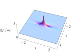
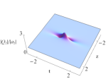
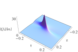
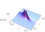
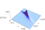
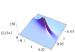
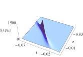
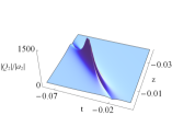
Figure 1: The top panel shows the fundamental rogue wave dynamics of our solutions (2), obtained with the parameters $a_{1}=2$, $a_{2}=1$, $z_{1}=3+i$, $z_{3}=0$, $z_{4}=3$ and $z_{2}=4$. The same is shown for different parameters $z_{2}=1/3$ (2nd row), $z_{2}=1/6$ (3rd row) and $z_{2}=12/100$ (4th row).

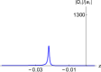
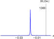
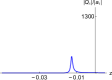
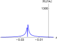
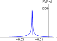
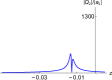
Figure 2: The fundamental rogue wave dynamics of our solutions, obtained with the parameters $a_{1}=2$, $a_{2}=1$, $z_{1}=3+i$, $z_{3}=0$, $z_{4}=3$, $z_{2}=12/100$ and $t=-0.06,-0.05,-0.04$ (from left to right). The modulus of each field is shown (top row: $Q_{1}$ and bottom row $Q_{2}$) normalized to its respective background amplitude.

In the remaining panels of the figure, depending on the relative values of the structural parameter $z_{2}$, the fundamental rogue wave solutions, still expressed by rational functions of the fourth degree, can remarkably reach an amplitude as high as a thousand times the background level. When $z_{2}=\frac{1}{3}$, it is noted that $Q_{1}$ and $Q_{2}$ reach an amplitude limit at least as high as $26$ times the background level. When $z_{2}=\frac{1}{6}$, it is noted that both components are at least over $110$ times the background level. When $z_{2}=\frac{12}{100}$, it is noted that $Q_{1}$ and $Q_{2}$ reach an amplitude limit as high as at least $1200$ times the background level. Besides, the $Q_{1}$ component has one peak, while the $Q_{2}$ component has two peaks. This is in line with the feature that such equations also admit the vector single peak-double peak solitons on top of a vanishing background 13 . For completeness, in Fig. 2, we illustrate the profile of the modulus of both spatial fields (divided by their respective backgrounds) near and at the instance of peak formation. We show how the fundamental rogue waves reach the ultra-high peak amplitude in both fields within a short time. It is worth noticing how the second component forms a peak first on one side of the first component maximum, subsequently symmetrizes and then the peak appears on the other side of the first component maximum. It is also relevant to note that when $|\lambda|<\sqrt{{a_{1}}^{2}-{a_{2}}^{2}}$, Akhmediev breathers arise in the model, which means that the solutions exhibit localization in $z$ but periodicity along $t$. On the other hand, when $|\lambda|>\sqrt{{a_{1}}^{2}-{a_{2}}^{2}}$, Kuznetsov-Ma solitons appear, which means that the solutions exhibit localization in $t$ but periodicity along $z$. Akhmediev breathers and Kuznetsov-Ma solitons with ultra-high peak amplitude are shown in Fig. 3.

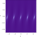
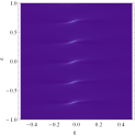
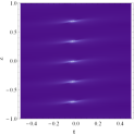
Figure 3: Space-time contour plots of vector breathers with $z_{1}=3+i$, $z_{2}=1/6$, $z_{3}=0$, $z_{4}=3$, $a_{1}=2$, $a_{2}=1$, $\lambda=i<\sqrt{3}i$ (Akhmediev breather in the top row) and $\lambda=2.5i>\sqrt{3}i$ (Kuznetsov-Ma soliton in the bottom row).

Now we show that such vector rogue waves could be generated in the modulation instability (MI) regime. We take the background solutions as $Q_{10}=a_{1}e^{i(kz+\omega t)}$ and $Q_{20}=ia_{2}e^{i(kz+\omega t)}$ with $k=2a_{1}^{2}-2a_{2}^{2}-\omega^{2}$. A perturbed nonlinear background can be written as $Q_{1}=(a_{1}+p_{1})e^{i(kz+\omega t)}$ and $Q_{1}=i(a_{2}+p_{2})e^{i(kz+\omega t)}$, where $p_{1}$ and $p_{2}$ are small perturbations. The $p_{1}$ and $p_{2}$ are $t$-periodic with frequency $\Omega$. Using linear stability analysis, we obtain the eigenvalues of the linear system as $\pm\sqrt{-4a_{1}^{2}\Omega^{2}+4a_{2}^{2}\Omega^{2}+\Omega^{4}}-2\omega\Omega$. When the eigenvalue has a negative imaginary part, MI arises, which means $a_{1}>a_{2}$. Therefore, when $|a_{1}|>|a_{2}|$, a baseband MI pr4 , which includes frequencies that are arbitrarily close to zero, is present, i.e., $0<\Omega^{2}<4a^{2}_{1}-4a^{2}_{2}$. In Fig. 4, we show the logarithmic gain plot $\ln G({\Omega})$ versus $\Omega$, where $G(\Omega)=\sqrt{+4a_{1}^{2}\Omega^{2}-4a_{2}^{2}\Omega^{2}-\Omega^{4}}$. The gain maximum is found to be $1.09861$ at $\Omega=1.73205$.

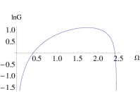
Figure 4: MI gain at $k=0,a_{1}=2,a_{2}=1$.

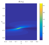
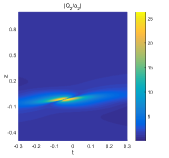
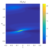
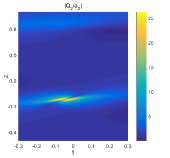
Figure 5: Numerical simulations of the $z-t$ evolution (shown through contour plots) of the fundamental rogue waves in Fig. 1 with $z_{2}=1/3$ without perturbation (upper row) and with $5\%$ white noise perturbation (bottom row).

We also use numerical simulations to investigate the robustness of these fundamental rogue waves in Fig. 5. Here, the split-step Fourier spectral method is used to deal with the spatial derivative operators and the fourth-order Runge-Kutta method is brought to bear to tackle the forward time marching of Eqs. (1). We can observe that both with (bottom row panels) and without (top row panels) imposing a $5\%$ white noise perturbation tt1 on top of the solutions with $z_{2}=1/3$ (2nd row of Fig. 1), the waveforms are found to robustly persist in the evolution dynamics. In the presence of a perturbation, due to the spontaneous MI of the homogeneous state, both fields develop an unstable background after the fundamental rogue wave propagation. Similar case scenarios have been explored for other values of the parameters (e.g. for the case of $z_{2}=1/6$ of the third row of Fig. 1) and the results of Fig. 5 have been found to be representative of the dynamical robustness of the states at hand.

Importantly, we even find that such unusual extremely high peak-amplitude fundamental rogue waves can be excited in a chaotic background field. To do this, we use the plane wave solutions as initial conditions at $z=0$, perturbed by random noise of a strength of $2\%$. Specifically, we multiply the plane waves in $Q_{1}$ and $Q_{2}$ by the factors $[1+0.02f_{j}(t)](j=1,2)$, respectively, where $f_{j}(t)$ are real random functions whose mean value is $0$ and variance is $1/3$. Besides, $f_{j}(t)$ are taken as Gaussian distributed and Gaussian correlated functions with the correlation length $1/2$ NJA2009 .

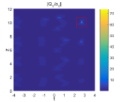
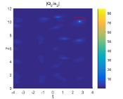
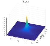
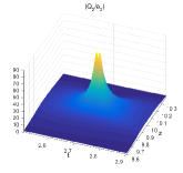
Figure 6: Numerical excitation of the fundamental rogue waves. The initial condition is a plane wave perturbed by $2\%$ random noise with $a_{1}=2$, $a_{2}=1$ and $f_{1}(t)\neq f_{2}(t)$: The amplitude evolution (upper row); The enlarged 3D plots of the high peak-amplitude vector rogue wave profiles highlighted by a surrounding box (bottom row).

We have examined a series of cases where $f_{1}(t)=f_{2}(t)$. In that case, the effective correlation built between the fields does not allow the maximal amplitude to be significantly larger than $3$. I.e., we are in an effective single-component NLS regime and while rogue waves are clearly discernible, they are not of the anomalously large amplitude variety created by the mechanism proposed herein. However, in Fig. 6, considering the same selection of model parameters as before, we select $f_{1}(t)$ and $f_{2}(t)$ to be different random variables (empirically, we find that even a small difference between the two is sufficient). Then, we see that some waves in the chaotic background clearly feature significant increase in their amplitudes. The parts selected by red boxes are enlarged in the corresponding mesh plots for the two fields of the bottom panel, revealing a high peak-amplitude vector rogue wave excited. Such a rogue wave is clearly distinguished from general higher-order rogue waves (superposition of fundamental rogue waves), arising in the form of suitable analytical solutions, e.g., in the realm of the single-component NLS model (2). Hence, this spontaneously emerging pattern within the chaotic background is a definitive manifestation of the type of wave pattern advocated in the present work. We attribute the key differences to the coherent coupling effect. Due to the existence of coherent coupling terms in Eqs. (1), the phase-dependent contribution (coherence) of plane waves in $Q_{1}$ and $Q_{2}$ plays an important role. Indeed, that coherent coupling is chiefly responsible for the presence of a single energy/mass-type conservation law as per Eq. (14). If $C=F=0$, then the two components individually conserve their energy. In that case, this type of two-component interplay of mutual growth leading in pairwise cancellation at the level of Eq. (14), yet indefinite growth at the level of each individual component is prohibited by the individual conservation laws. We thus argue that this mechanism and phenomenology is unique to this type of coherently coupled NLS models and thus not encountered in the settings previously considered.

4. Conclusions/Future Work

In the present work, we have unveiled an unprecedented mechanism, to the best of our knowledge, regarding the formation of arbitrary amplitude rogue waves. Within this scenario, we have explained the role of coherent coupling terms, in conjunction with an unconventional (single) energy conservation law bearing indefinite sign between the energies of individual components. As a result, in a prototypical (within this class of features) NLS model inspired by the examination of multiple polarizations in a nonlinear fiber, we have shown that vector fundamental rogue waves (in both components) of such coupled equations could reach peak amplitudes of the order of a thousand times the background level. The fundamental solutions we consider here are rational solutions of fourth degree. Their periodic extensions in the $z$ (Kuznetsov-Ma soliton) and $t$ (Akhmediev breather) variables were also identified and illustrated. Furthermore, we have numerically confirmed that such unusual, extremely high peak-amplitude vector fundamental rogue waves are robust even under moderate perturbations. Last but not least, we have confirmed that such vector fundamental rogue waves could be excited in a chaotic background field, i.e., that such excitations indeed spontaneously arise in dynamical simulations against the backdrop of an unstable background. In as far as we can tell, the key mechanism elucidated here enables the significant eclipsing of the highest amplitude of previously reported rogue waves. This most naturally poses the question of whether a direct (or an engineered) observation of this phenomenon can arise and can be accordingly harnessed. From a theoretical perspective numerous extensions of the ideas reported herein can also be pursued including the extension and numerical identification of such states beyond the integrable limit considered herein, utilizing, e.g., recent ideas such as those of cory . Another extension of interest is to consider two-dimensional variants of the present model and whether rogue wave of the present type can be identified in suitable generalizations of settings related to the Davey-Stewartson and Benney-Roskes models where two-dimensional rogue patterns were recently considered in jingsong .

Acknowledgments
       This work has been supported by the National Natural Science Foundation of China under Grant Nos.61705006, 11305060 and 11947230, by the Fundamental Research Funds of the Central Universities (Nos.230201606500048 and 2018MS048), and by the China Postdoctoral Science Foundation (No. 2019M660430). This material is based upon work supported by the US National Science Foundation under Grants No. PHY-1602994 and DMS-1809074 (PGK). PGK also acknowledges support from the Leverhulme Trust via a Visiting Fellowship and thanks the Mathematical Institute of the University of Oxford for its hospitality during part of this work.

*liueli@126.com

Appendix:
       The fundamental solutions (2) with the parameters $a_{1}=2$, $a_{2}=1$, $z_{1}=3+i$, $z_{3}=0$ and $z_{4}=3$ are given as:

$$\hskip 142.26378ptQ_{1}(z,t)=-2e^{6iz}\frac{G_{1}}{F},\quad Q_{2}(z,t)=-e^{6iz}\frac{G_{2}}{F},$$

$$G_{1}=36z_{2}^{4}t^{4}+288\sqrt{3}z_{2}^{3}t^{4}-144\sqrt{3}z_{2}^{2}t^{4}+2952z_{2}^{2}t^{4}+144\sqrt{3}t^{4}+4896\sqrt{3}z_{2}t^{4}-1728z_{2}t^{4}$$

$$+16020t^{4}+24\sqrt{3}z_{2}^{4}t^{3}+288z_{2}^{3}t^{3}+384\sqrt{3}z_{2}^{2}t^{3}-144z_{2}^{2}t^{3}+456\sqrt{3}t^{3}-288z_{2}t^{3}+2736t^{3}$$

$$+864z^{2}z_{2}^{4}t^{2}-144izz_{2}^{4}t^{2}+12z_{2}^{4}t^{2}-1152i\sqrt{3}zz_{2}^{3}t^{2}+6912z^{2}\sqrt{3}z_{2}^{3}t^{2}-36\sqrt{3}z_{2}^{3}t^{2}+384480z^{2}t^{2}$$

$$-3456\sqrt{3}z^{2}z_{2}^{2}t^{2}+70848z^{2}z_{2}^{2}t^{2}-11808izz_{2}^{2}t^{2}-(864-576i)\sqrt{3}zz_{2}^{2}t^{2}+72i\sqrt{3}z_{2}^{2}t^{2}-456z_{2}^{2}t^{2}$$

$$+(444-1296i)t^{2}+(15552-64080i)zt^{2}-(864+576i)\sqrt{3}zt^{2}+3456z^{2}\sqrt{3}t^{2}+72i\sqrt{3}t^{2}$$

$$-41472z^{2}z_{2}t^{2}+6912izz_{2}t^{2}+117504z^{2}\sqrt{3}z_{2}t^{2}-(612+288i)\sqrt{3}z_{2}t^{2}+(3456-19584i)z\sqrt{3}z_{2}t^{2}$$

$$+216z_{2}t^{2}-48i\sqrt{3}zz_{2}^{4}t+288z^{2}\sqrt{3}z_{2}^{4}t+3456z^{2}z_{2}^{3}t-576izz_{2}^{3}t-36z_{2}^{3}t+32832z^{2}t-1728z^{2}z_{2}^{2}t$$

$$+288izz_{2}^{2}t-768i\sqrt{3}zz_{2}^{2}t+4608z^{2}\sqrt{3}z_{2}^{2}t-5472izt-912i\sqrt{3}zt+5472z^{2}\sqrt{3}t-3456z^{2}z_{2}t$$

$$+(36-216i)z_{2}t+(2592+576i)zz_{2}t-216i\sqrt{3}z_{2}t+2592z\sqrt{3}z_{2}t+2306880z^{4}+5184z^{4}z_{2}^{4}$$

$$-1728iz^{3}z_{2}^{4}-24izz_{2}^{4}-z_{2}^{4}+(186624-768960i)z^{3}-(10368+6912i)\sqrt{3}z^{3}-13824i\sqrt{3}z^{3}z_{2}^{3}$$

$$-720\sqrt{3}z^{2}z_{2}^{3}-72i\sqrt{3}zz_{2}^{3}+41472z^{4}\sqrt{3}z_{2}^{3}-6\sqrt{3}z_{2}^{3}-(58752+46656i)z^{2}-(576-2592i)\sqrt{3}z^{2}$$

$$-20736\sqrt{3}z^{4}z_{2}^{2}+425088z^{4}z_{2}^{2}-141696iz^{3}z_{2}^{2}-(10368-6912i)\sqrt{3}z^{3}z_{2}^{2}-6912z^{2}z_{2}^{2}$$

$$-816izz_{2}^{2}+(576+2592i)z^{2}\sqrt{3}z_{2}^{2}+144z\sqrt{3}z_{2}^{2}-34z_{2}^{2}-(2592+888i)z+20736z^{4}\sqrt{3}+144z\sqrt{3}$$

$$-248832z^{4}z_{2}+82944iz^{3}z_{2}-(12240+10368i)\sqrt{3}z^{2}z_{2}+4320z^{2}z_{2}+432izz_{2}-(144+1224i)\sqrt{3}zz_{2}$$

$$+705024z^{4}\sqrt{3}z_{2}+(41472-235008i)z^{3}\sqrt{3}z_{2}-(102+36i)\sqrt{3}z_{2}-1,$$

$$F=36t^{4}z_{2}^{4}+288\sqrt{3}t^{4}z_{2}^{3}-144\sqrt{3}t^{4}z_{2}^{2}+2952t^{4}z_{2}^{2}+4896\sqrt{3}t^{4}z_{2}-1728t^{4}z_{2}+144\sqrt{3}t^{4}+16020t^{4}$$

$$+24\sqrt{3}t^{3}z_{2}^{4}+288t^{3}z_{2}^{3}+384\sqrt{3}t^{3}z_{2}^{2}-144t^{3}z_{2}^{2}-288t^{3}z_{2}+456\sqrt{3}t^{3}+2736t^{3}+864t^{2}z^{2}z_{2}^{4}$$

$$+6912\sqrt{3}t^{2}z^{2}z_{2}^{3}+384480t^{2}z^{2}-3456\sqrt{3}t^{2}z^{2}z_{2}^{2}+70848t^{2}z^{2}z_{2}^{2}+3456\sqrt{3}t^{2}z^{2}-41472t^{2}z^{2}z_{2}$$

$$+117504\sqrt{3}t^{2}z^{2}z_{2}+24t^{2}z_{2}^{4}+48\sqrt{3}t^{2}z_{2}^{3}-864\sqrt{3}t^{2}zz_{2}^{2}-24\sqrt{3}t^{2}z_{2}^{2}+384t^{2}z_{2}^{2}$$

$$-864\sqrt{3}t^{2}z+15552t^{2}z+3456\sqrt{3}t^{2}zz_{2}+816\sqrt{3}t^{2}z_{2}+24\sqrt{3}t^{2}+4344t^{2}+288\sqrt{3}tz^{2}z_{2}^{4}+3456tz^{2}z_{2}^{3}$$

$$+32832tz^{2}-1728tz^{2}z_{2}^{2}+4608\sqrt{3}tz^{2}z_{2}^{2}+5472\sqrt{3}tz^{2}-3456tz^{2}z_{2}+4\sqrt{3}tz_{2}^{4}-864tzz_{2}^{2}+64\sqrt{3}tz_{2}^{2}$$

$$-16416tz+3456tzz_{2}+76\sqrt{3}t+2306880z^{4}+5184z^{4}z_{2}^{4}+41472\sqrt{3}z^{4}z_{2}^{3}-20736\sqrt{3}z^{4}z_{2}^{2}+425088z^{4}z_{2}^{2}$$

$$+20736\sqrt{3}z^{4}-248832z^{4}z_{2}+705024\sqrt{3}z^{4}z_{2}-10368\sqrt{3}z^{3}+186624z^{3}-10368\sqrt{3}z^{3}z_{2}^{2}+41472\sqrt{3}z^{3}z_{2}$$

$$+144z^{2}z_{2}^{4}+576\sqrt{3}z^{2}z_{2}^{3}+22608z^{2}-288\sqrt{3}z^{2}z_{2}^{2}+6624z^{2}z_{2}^{2}+288\sqrt{3}z^{2}$$

$$-6912z^{2}z_{2}+9792\sqrt{3}z^{2}z_{2}+z_{2}^{4}-144\sqrt{3}zz_{2}^{2}+34z_{2}^{2}-144\sqrt{3}z+576\sqrt{3}zz_{2}+1.$$

$$G_{2}=36iz_{2}^{4}t^{4}+288i\sqrt{3}z_{2}^{3}t^{4}+2952iz_{2}^{2}t^{4}-144i\sqrt{3}z_{2}^{2}t^{4}+16020it^{4}+144i\sqrt{3}t^{4}-1728iz_{2}t^{4}$$

$$+4896i\sqrt{3}z_{2}t^{4}+24i\sqrt{3}z_{2}^{4}t^{3}+288iz_{2}^{3}t^{3}-144iz_{2}^{2}t^{3}+384i\sqrt{3}z_{2}^{2}t^{3}+2736it^{3}+456i\sqrt{3}t^{3}-288iz_{2}t^{3}$$

$$+864iz^{2}z_{2}^{4}t^{2}+12iz_{2}^{4}t^{2}+144zz_{2}^{4}t^{2}+6912iz^{2}\sqrt{3}z_{2}^{3}t^{2}+1152z\sqrt{3}z_{2}^{3}t^{2}+384480iz^{2}t^{2}+70848iz^{2}z_{2}^{2}t^{2}$$

$$-3456i\sqrt{3}z^{2}z_{2}^{2}t^{2}-24iz_{2}^{2}t^{2}-(576+864i)\sqrt{3}zz_{2}^{2}t^{2}+11808zz_{2}^{2}t^{2}-(72+72i)\sqrt{3}z_{2}^{2}t^{2}+(1296+4764i)t^{2}$$

$$+(64080+15552i)zt^{2}+3456iz^{2}\sqrt{3}t^{2}-(72-72i)\sqrt{3}t^{2}+(576-864i)z\sqrt{3}t^{2}-41472iz^{2}z_{2}t^{2}-864iz_{2}t^{2}$$

$$-6912zz_{2}t^{2}+117504iz^{2}\sqrt{3}z_{2}t^{2}+(19584+3456i)z\sqrt{3}z_{2}t^{2}+288\sqrt{3}z_{2}t^{2}+288iz^{2}\sqrt{3}z_{2}^{4}t$$

$$+48z\sqrt{3}z_{2}^{4}t+3456iz^{2}z_{2}^{3}t+576zz_{2}^{3}t+32832iz^{2}t-1728iz^{2}z_{2}^{2}t+(216-72i)z_{2}^{2}t-(288-2592i)zz_{2}^{2}t$$

$$+4608iz^{2}\sqrt{3}z_{2}^{2}t+768z\sqrt{3}z_{2}^{2}t+(4104+1368i)t+(5472+49248i)zt+5472iz^{2}\sqrt{3}t+912z\sqrt{3}t$$

$$-3456iz^{2}z_{2}t-576zz_{2}t+10368iz\sqrt{3}z_{2}t+864\sqrt{3}z_{2}t+2306880iz^{4}+5184iz^{4}z_{2}^{4}+1728z^{3}z_{2}^{4}-iz_{2}^{4}$$

$$+24zz_{2}^{4}+(768960+186624i)z^{3}-1152i\sqrt{3}z^{2}z_{2}^{3}+41472iz^{4}\sqrt{3}z_{2}^{3}+13824z^{3}\sqrt{3}z_{2}^{3}+(46656-110592i)z^{2}$$

$$-(2592+1440i)\sqrt{3}z^{2}+425088iz^{4}z_{2}^{2}-20736i\sqrt{3}z^{4}z_{2}^{2}-(6912+10368i)\sqrt{3}z^{3}z_{2}^{2}$$

$$+141696z^{3}z_{2}^{2}-12096iz^{2}z_{2}^{2}-(2592-1440i)\sqrt{3}z^{2}z_{2}^{2}-34iz_{2}^{2}-48zz_{2}^{2}+(36-12i)\sqrt{3}z_{2}^{2}$$

$$+(144+576i)z\sqrt{3}z_{2}^{2}-i-(7752+2592i)z-(144-576i)\sqrt{3}z+20736iz^{4}\sqrt{3}+(6912-10368i)z^{3}\sqrt{3}$$

$$+(36+12i)\sqrt{3}-248832iz^{4}z_{2}-82944z^{3}z_{2}+17280iz^{2}z_{2}-576i\sqrt{3}zz_{2}+1728zz_{2}+705024iz^{4}\sqrt{3}z_{2}$$

$$+(235008+41472i)z^{3}\sqrt{3}z_{2}+(10368-19584i)z^{2}\sqrt{3}z_{2},$$

References

(1)
C. Kharif, E. Pelinovsky, and A. Slunyaev, Rogue Waves in the Ocean (Springer, Heidelberg, New York, 2009).
(2)
A. R. Osborne, Nonlinear Ocean Waves and the Inverse Scattering Transform (Elsevier, Amsterdam, 2010).
(3)
A. Chabchoub, N. P. Hoffmann, and N. Akhmediev, Phys. Rev. Lett. 106, 204502 (2011).
(4)
J.M. Dudley, F. Dias, M. Erkintalo, and G. Genty, Nat. Photonics 8, 755 (2014).
(5)
B. Kibler, J. Fatome, C. Finot, G. Millot, F. Dias, G. Genty,
N. Akhmediev, and J. M. Dudley, Nat. Phys. 6, 790 (2010).
(6)
A. Tikan, C. Billet, G. El, A. Tovbis, M. Bertola, T.
Sylvestre, F. Gustave, S. Randoux, G. Genty, P. Suret,
and J. M. Dudley, Phys. Rev. Lett. 119, 033901 (2017).
(7)
D. R. Solli, C. Ropers, P. Koonath, and B. Jalali, Nature 450, 1054 (2007).
(8)
N. Akhmediev, J. M. Dudley, D. R. Solli, and S. K. Turitsyn,
J. Opt. 15, 060201 (2013).
(9)
M. Onorato, S. Residori, U. Bortolozzo, A. Montina, and
F. T. Arecchi, Phys. Rep. 528, 47 (2013).
(10)
F. Baronio, M. Conforti, A. Degasperis and S, Lombardo,
Phys. Rev. Lett. 111, 114101 (2013).
(11)
F. Baronio, S. Chen, P. Grelu, S. Wabnitz, and M. Conforti,
Phys. Rev. A 91, 033804 (2015).
(12)
F. Baronio, M. Conforti, A. Degasperis, S. Lombardo, M. Onorato, and
S. Wabnitz, Phys. Rev. Lett. 113, 034101 (2014).
(13)
S. Chen, F. Baronio, J. M. Soto-Crespo, P. Grelu, M. Conforti, and
S. Wabnitz, Phys. Rev. A 92, 033847 (2015).
(14)
F. Baronio, B. Frisquet, S. Chen, G. Millot, S. Wabnitz, and
B. Kibler, Phys. Rev. A 97, 013852 (2018).
(15)
D. H. Peregrine, J. Aust. Math. Soc. Series B, Appl. Math. 25, 16 (1983).
(16)
A. Chabchoub, N. P. Hoffmann, and N. Akhmediev, Phys.
Rev. Lett. 106, 204502 (2011).
(17)
H. Bailung, S. K. Sharma, and Y. Nakamura, Phys. Rev.
Lett. 107, 255005 (2011).
(18)
S. Chen, Phys. Rev. E 88, 023202 (2013).
(19)
W. R. Sun, B. Tian, Y. Jiang, and H. L. Zhen, Phys. Rev. E 91, 023205 (2015).
(20)
W. R. Sun, and L. Wang, P. Roy. Soc. A 474, 20170276 (2018).
(21)
L. Liu, B. Tian, Y. Q. Yuan, and Z. Du, Phys. Rev. E 97, 052217 (2018).
(22)
L. C. Zhao, Sh. C. Li, and L. Ling, Phys. Rev. E 93, 032215 (2016).
(23)
J. Ieda, T. Miyakawa, and M. Wadati, Phys. Rev. Lett. 93, 194102
(2004).
(24)
N. Akhmediev, A. Ankiewicz, and J. M. Soto-Crespo, Phys. Rev. E 80, 026601 (2009).
(25)
A. Chabchoub, N. Hoffmann, M. Onorato, and N. Akhmediev, Phys. Rev. X
2, 011015 (2012).
(26)
M. Narhi, B. Wetzel, C. Billet, S. Toenger, T. Sylvestre,
J.-M. Merolla, R. Morandotti, F. Dias, G. Genty, and J. M.
Dudley, Nat. Commun. 7, 13675 (2016).
(27)
S. Chen, Y. Ye, J. M. Soto-Crespo, P. Grelu, and F. Baronio,
Phys. Rev. Lett. 121, 104101 (2018).
(28)
S. Chen, C. Pan, P. Grelu, F. Baronio, and N. Akhmediev,
Phys. Rev. Lett. 124, 113901 (2020).
(29) M.J. Ablowitz, B. Prinari and A.D. Trubatch,
Discrete and Continuous Nonlinear Schrödinger Systems,
Cambridge University Press (Cambridge, 2004).