Inhomogeneous XX spin chains and quasi-exactly solvable models

Abstract

We establish a direct connection between inhomogeneous XX spin chains (or free fermion systems with nearest-neighbors hopping) and certain QES models on the line giving rise to a family of weakly orthogonal polynomials. We classify all such models and their associated XX chains, which include two families related to the Lamé (finite gap) quantum potential on the line. For one of these chains, we numerically compute the Rényi bipartite entanglement entropy at half filling and derive an asymptotic approximation thereof by studying the model’s continuum limit, which turns out to describe a massless Dirac fermion on a suitably curved background. We show that the leading behavior of the entropy is that of a $c=1$ critical system, although there is a subleading $\log(\log N)$ correction (where $N$ is the number of sites) unusual in this type of models.

Keywords: spin chains, ladders and planes; solvable lattice models; entanglement in extended quantum systems; conformal field theory.

1 Introduction

Inhomogeneous XX spin chains —or, equivalently, systems of free spinless fermions with nearest-neighbors hopping— have recently received considerable attention due to their remarkable entanglement properties. Indeed, the critical phases of these models are effectively described by $1+1$ dimensional conformal field theories (CFTs), whose entanglement has been extensively studied using standard field-theoretic techniques (see, e.g., [1, 2]). In particular, the single-block Rényi entanglement entropy of $1+1$ dimensional CFTs features a characteristic logarithmic growth with the block length $L$, rather than the usual linear growth of thermodynamic entropy. Thus it is to be expected that the entanglement entropy of critical inhomogeneous XX chains also scales proportionally to $\log L$ as $L$ goes to infinity; in particular, the model’s central charge can be inferred from the proportionality constant multiplying $\log L$ in the asymptotic formula for the entropy. The entanglement entropy of the homogeneous XX chain has in fact been thoroughly studied in the open, closed and (semi-)infinite cases [3, 4, 5], as well as for subsystems consisting of more than one block [6, 7, 8, 9, 10, 11]. In all cases the leading behavior of the Rényi entropy has been found to be logarithmic, with the expected central charge $c=1$ of a free fermion CFT.

The asymptotic behavior of the entanglement entropy of truly inhomogeneous XX chains is much harder to establish, since in this case the correlation matrix is neither Toeplitz nor Toeplitz plus Hankel, so that the standard techniques based on using proved cases of the Fisher–Hartwig conjecture [12, 13, 14] to approximate the characteristic polynomial of the latter matrix for large $L$ cannot be applied. However, in some cases an approximation of the entanglement entropy can be found by exploiting the model’s connection with a suitable CFT. This idea has been successfully applied to the so-called rainbow chain [15], whose hopping amplitudes decay exponentially outwards from both sides of the chain’s center. More precisely, it was first shown in Ref. [16] that in the continuum limit the rainbow chain’s Hamiltonian tends to that of a massless Dirac fermion in a suitably curved $1+1$ dimensional background, whose metric’s conformal factor is proportional to the square of the chain’s hopping amplitude. Using the results in Ref. [17] for the entanglement entropy of the latter model, the authors in Ref. [18] derived an asymptotic formula for the entanglement entropy of the rainbow chain which is in excellent agreement with the numerical data.

Another key feature of inhomogeneous XX chains is their close connection to the classical theory of orthogonal polynomials, stemming from the fact that the matrix of the system’s single-particle (fermionic) Hamiltonian in the position basis is real, symmetric and tridiagonal, and thus its entries can be used to define a three-term recursion relation determining a (finite) orthogonal polynomial system. In this way a one-to-one correspondence between inhomogeneous XX chains and orthogonal polynomial families is established. In fact, the zeros of the last polynomial in the family coincide with the chain’s single particle energies, and the chain’s complete spectrum is obtained by exciting an arbitrary number of these single particle states. This close connection between inhomogeneous XX chains and orthogonal polynomials was used, for instance, to characterize chains of this type with perfect state transfer [19, 20, 21] or, more recently, to construct a tridiagonal matrix commuting with the hopping matrix of the entanglement Hamiltonian of several inhomogeneous XX chains constructed from well-known families of discrete (finite) polynomial systems [22].

The theory of orthogonal polynomials has also close connections to another class of one-dimensional (one body) quantum systems, namely quasi-exactly solvable (QES) dynamical models on the line. In general, these models are characterized by the fact that a subset of the spectrum can be found through algebraic procedures. The prototypical examples of QES models are those whose Hamiltonian can be expressed as a quadratic polynomial in the generators of the standard spin $(N-1)/2$ representation of the $\mathrm{sl}(2)$ algebra in terms of first-order differential operators [23, 24, 25, 26]. After an appropriate (pseudo-)gauge transformation, the (formal) eigenfunctions of these models can be expressed as power series in a suitable variable $z$, whose coefficients $P_{n}(E)$ depend polynomially on the energy $E$ [27]. In many cases, these polynomials satisfy a three-term recursion relation, and are therefore orthogonal with respect to a suitable measure [28]. Moreover, for certain values of the parameters in the Hamiltonian there is a positive integer $N$ such that the polynomials $P_{n}(E)$ with $n\geqslant N$ are divisible by $P_{N}(E)$. Thus the model becomes QES, as the gauged Hamiltonian obviously admits polynomial eigenfunctions of degree up to $N-1$ in the variable $z$ with energies equal to the $N$ zeros of the critical polynomial $P_{N}$. Furthermore, in this case the polynomial family $\{P_{n}(E)\}_{n=0}^{\infty}$ is weakly orthogonal, since it can be shown that the polynomials of degree greater than or equal to $N$ have zero norm.

The aim of this paper is to classify all the inhomogeneous XX spin chains associated with a QES model on the line, in the sense that they share the same family of orthogonal polynomials. In other words, we look for chains whose parameters (hopping amplitudes and on-site energies) are derived from the coefficients of the three-term recursion relation of the weakly orthogonal polynomial system associated to a QES model. To this end, we first show that there are exactly six inequivalent types of QES models on the line giving rise to a weakly orthogonal polynomial system, up to projective transformations. We then prove that any XX chain with the above property is isomorphic to one of the six chains constructed from the latter canonical forms. One of the characteristic properties of these chains is that their hopping amplitudes and on-site energies are algebraic functions of the site index $n$. Remarkably, this is also the case for the models recently constructed from classical Krawtchouk and dual Hahn polynomials in Refs. [19, 20, 22], although they all differ from the six new chains introduced in this work. Among these new models there are, in particular, several chains constructed from different QES realizations of the celebrated Lamé (finite gap) potential [29].

As remarked in Ref. [22], from the knowledge of the orthogonal polynomial system defined by an inhomogeneous XX chain it is straightforward to find an explicit expression for the corresponding free fermion system’s correlation matrix, whose eigenvalues yield the model’s entanglement entropy [30, 31]. This is in fact a very efficient method for computing the entanglement entropy (in fact, the whole entanglement spectrum), since it is based on diagonalizing an $L\times L$ matrix instead of the $2^{L}\times 2^{L}$ reduced density matrix. We have applied this idea to compute the Rényi entanglement entropy of one of the new inhomogeneous XX spin chains constructed from the Lamé potential, whose on-site energies are all zero. Using the method developed in Ref. [18], we have constructed the continuum limit of the latter chain, which again describes a massless Dirac fermion in a curved $1+1$ dimensional background. In this way we have obtained an asymptotic formula for the chain’s Rényi entanglement entropy when the number of sites goes to infinity, which is shown to be in excellent agreement with the numerical results for up to $600$ sites. In particular, this confirms that the model has a critical phase with $c=1$, as expected.

This paper is organized as follows. In Section 2 we present the models and discuss their connection with Jacobi (tridiagonal symmetric) matrices. Section 3 includes a brief summary of several fundamental results from the classical theory of orthogonal polynomials of interest in the sequel. In particular, we deduce a closed formula for the weights of a finite (or weakly orthogonal) polynomial system in terms of the zeros of the critical polynomial. In Section 4 we outline the application of these results to the diagonalization of the hopping matrix of inhomogeneous XX chains (or free fermion systems), establishing a one-to-one correspondence between orthogonal polynomial systems and inhomogeneous XX spin chains. Section 5 contains a concise review of QES models on the line constructed from the $\mathrm{sl}(2)$ algebra, with special emphasis on their connection with weakly orthogonal polynomial systems. In Section 6 we present our classification of all inequivalent XX spin chains constructed from the orthogonal polynomial families determined by QES models on the line. Section 7 is devoted to the study of the Rényi entanglement entropy of one of the new XX spin chains introduced in the previous section, connected to a QES realization of the Lamé potential. The paper ends with a technical appendix which provides the complete details of the classification presented in Section 6.

2 Inhomogeneous XX spin chains

Assuming conservation of the total number of fermions, the most general free fermion Hamiltonian with nearest-neighbors hopping can be written as

$$H=\sum_{n=0}^{N-2}J_{n}\big{(}\rme^{\mathrm{i}\alpha_{n}}{\hat{c}}^{\dagger}_{n}\hat{c}_{n+1}+\rme^{-\mathrm{i}\alpha_{n}}\hat{c}^{\dagger}_{n+1}\hat{c}_{n}\big{)}+\sum_{n=0}^{N-1}B_{n}\hat{c}^{\dagger}_{n}\hat{c}_{n}\,,$$ (2.1)

where $J_{n}\geqslant 0$, $\alpha_{n},B_{n}\in{\mathbb{R}}$ and the operators $\{\hat{c}_{n},\hat{c}^{\dagger}_{n}\}_{n=0}^{N-1}$ are a family of fermionic operators satisfying the canonical anticommutation relations (CAR)

$$\{\hat{c}_{n},\hat{c}_{m}\}=\{\hat{c}^{\dagger}_{n},\hat{c}^{\dagger}_{m}\}=0\,,\qquad\{\hat{c}_{n},\hat{c}^{\dagger}_{m}\}=\delta_{nm}\,.$$

As a matter of fact, the latter Hamiltonian can be brought to a simpler canonical form by introducing the equivalent family of fermionic operators

$$c_{n}=\rme^{\mathrm{i}\beta_{n}}\hat{c}_{n}\,,$$

with suitably chosen phases $\beta_{n}\in{\mathbb{R}}$. Indeed, we clearly have

$$H=\sum_{n=0}^{N-2}J_{n}\big{(}\rme^{\mathrm{i}\alpha_{n}}\rme^{\mathrm{i}(\beta_{n}-\beta_{n+1})}c^{\dagger}_{n}c_{n+1}+\rme^{-\mathrm{i}\alpha_{n}}\rme^{-\mathrm{i}(\beta_{n}-\beta_{n+1})}c^{\dagger}_{n+1}c_{n}\big{)}+\sum_{n=0}^{N-1}B_{n}c^{\dagger}_{n}c_{n}\,,$$

so that choosing $\beta_{n+1}-\beta_{n}=\alpha_{n}$, i.e.,

$$\beta_{n}=\sum_{j=0}^{n-1}\alpha_{j}\,,$$

the original Hamiltonian (2.1) reduces to

$$H=\sum_{n=0}^{N-2}J_{n}(c^{\dagger}_{n}c_{n+1}+c^{\dagger}_{n+1}c_{n})+\sum_{n=0}^{N-1}B_{n}c^{\dagger}_{n}c_{n}\,.$$ (2.2)

This model describes a system of $N$ hopping spinless fermions with real hopping amplitudes $J_{n}$ and chemical potentials (or on-site energies) $B_{n}$. The latter Hamiltonian obviously commutes with the total fermion number operator

$${\mathcal{N}}=\sum_{n=0}^{N-1}c^{\dagger}_{n}c_{n}\,,$$

so that the number of fermions is indeed conserved. In what follows we shall always assume that the hopping amplitudes do not vanish, so that

$$J_{n}>0\,,\qquad 0\leqslant n\leqslant N-2\,.$$ (2.3)

Note that, by the previous observation, the latter model is trivially equivalent to the analogous one with nonvanishing (positive or negative) hopping amplitudes $\varepsilon_{n}J_{n}$ with arbitrary signs $\varepsilon_{n}\in\{\pm 1\}$.

As is well known, under the Jordan–Wigner transformation

$$c_{n}=\prod_{k=0}^{n-1}\sigma_{k}^{z}\cdot\sigma_{n}^{+}\,,\qquad 0\leqslant n\leqslant N-1\,,$$ (2.4)

where $\sigma_{n}^{\alpha}$ (with $\alpha=x,y,z$) denotes the Pauli matrix $\sigma^{\alpha}$ acting on the $n$-th site and $\sigma^{\pm}_{\alpha}=(\sigma^{x}_{\alpha}\pm\mathrm{i}\sigma^{y}_{\alpha})/2$, the Hamiltonian (2.2) is transformed into the spin $1/2$ open XX chain Hamiltonian

$$H=\frac{1}{2}\sum_{n=0}^{N-2}J_{n}(\sigma_{n}^{x}\sigma_{n+1}^{x}+\sigma_{n}^{y}\sigma_{n+1}^{y})+\frac{1}{2}\sum_{n=0}^{N-1}B_{n}(1-\sigma_{n}^{z})\,.$$ (2.5)

Thus the models (2.2) and (2.5) can be regarded as essentially equivalent. In particular, the fermionic vacuum $|0\rangle$ corresponds to the reference state $|\uparrow\cdots\uparrow\rangle$ with all spins up, while the general fermionic state

$$c^{\dagger}_{n_{0}}\cdots c^{\dagger}_{n_{k}}|0\rangle\,,\qquad 0\leqslant n_{0}<\cdots<n_{k}\leqslant N-1\,,$$

is easily seen to correspond to the state

$$\sigma_{n_{0}}^{-}\cdots\sigma_{n_{k}}^{-}|\uparrow\cdots\uparrow\rangle$$

with flipped spins at positions $n_{0}<\cdots<n_{k}$. Note also in this respect that the transformation

$$c_{n}\mapsto\rme^{-\mathrm{i}\beta_{n}}c_{n}\,,$$

with $\beta_{n}$ real, corresponds to

$$\sigma_{n}^{\pm}\mapsto\rme^{\pm\mathrm{i}\beta_{n}}\sigma_{n}^{\pm},\qquad\sigma_{n}^{z}\mapsto\sigma_{n}^{z}\,,$$

which clearly preserves the commutation relations of the Pauli matrices. In what follows we shall mostly work with the fermionic model (2.2), our results being easily translated to the XX spin chain (2.5) by the previous considerations.

Let $H_{1}$ denote the restriction of the fermionic Hamiltonian $H$ in Eq. (2.2) to the subspace of one-particle states, a basis of which consists of the states

$$|n\rangle:=c^{\dagger}_{n}|0\rangle\,,\qquad 0\leqslant n\leqslant N-1\,,$$ (2.6)

with a single fermion at each site $n$. The matrix $\mathsf{H}=(H_{nm})_{n,m=0}^{N-1}$ of $H_{1}$ in the position basis (2.6) has matrix elements

$$H_{nm}=\langle n|H|m\rangle=J_{n}\delta_{m,n+1}+J_{n-1}\delta_{m,n-1}+B_{n}\delta_{nm}\,,$$ (2.7)

so that $\mathsf{H}$ is the $N\times N$ tridiagonal matrix

$$\mathsf{H}=\left(\begin{array}[]{cccccccc}B_{0}&J_{0}&0&0&\cdots&0&0&0\\ J_{0}&B_{1}&J_{1}&0&\cdots&0&0&0\\ 0&J_{1}&B_{2}&J_{2}&\cdots&0&0&0\\ \cdot&\cdot&\cdot&\cdot&\cdots&\cdot&\cdot&\cdot\\ 0&0&0&0&\cdots&J_{N-3}&B_{N-2}&J_{N-2}\\ 0&0&0&0&\cdots&0&J_{N-2}&B_{N-1}\end{array}\right)\,.$$ (2.8)

Note that in terms of this matrix the full Hamiltonian $H$ can be expressed in matrix notation as

$$H=\mathsf{C}^{\dagger}\mathsf{H}\mathsf{C}\,,$$ (2.9)

where $\mathsf{C}=(c_{0}\dots c_{N-1})^{T}$ and $\mathsf{C}^{\dagger}=(c^{\dagger}_{0}\dots c^{\dagger}_{N-1})$. Since $\mathsf{H}$ is real symmetric, it can be diagonalized by means of a real orthogonal transformation $\Phi$, i.e.,

$$\Phi^{T}\mathsf{H}\Phi=\mathop{\rm diag}\nolimits(E_{0},\dots,E_{N-1})\,,$$ (2.10)

where $E_{0}\leqslant\cdots\leqslant E_{N-1}$ are the (real) eigenvalues of $\mathsf{H}$. Let

$$\Phi_{nk}=:\phi_{n}(E_{k})\,,$$

an define a new set of fermionic operators $\tilde{c}_{n}$ by

$$\tilde{c}_{k}:=\sum_{n=0}^{N-1}\phi_{n}(E_{k})c_{n}\,,\qquad 0\leqslant k\leqslant N-1,$$ (2.11)

which satisfy the CAR on account of the orthogonal character of $\Phi$. Since $\widetilde{\mathsf{C}}=\Phi^{T}\mathsf{C}$, from Eqs. (2.9)-(2.10) it follows that

$$H=\widetilde{\mathsf{C}}^{\dagger}(\Phi^{T}\mathsf{H}\Phi)\widetilde{\mathsf{C}}=\sum_{n=0}^{N-1}E_{k}\tilde{c}^{\dagger}_{n}\tilde{c}_{n}\,.$$ (2.12)

Thus the full Hamiltonian $H$ is diagonal in the basis consisting of the states

$$\tilde{c}^{\dagger}_{n_{0}}\cdots\tilde{c}_{n_{k}}^{\dagger}|0\rangle\,,\qquad 0\leqslant n_{0}<\cdots<n_{k}\leqslant N-1\,,$$ (2.13)

whose corresponding energy is given by

$$E(n_{0},\dots,n_{k})=\sum_{j=0}^{k}E_{n_{j}}\,.$$ (2.14)

In particular, the states $\tilde{c}^{\dagger}_{k}|0\rangle$ (with $0\leqslant k\leqslant N-1$) are single-fermion excitation modes with energy $E_{k}$. Note, finally, that Eq. (2.10) is equivalent to the system of $N$ equations

$$\sum_{m=0}^{N-1}H_{nm}\phi_{m}(E_{k})=E_{k}\phi_{n}(E_{k})\,,$$

or, taking (2.7) into account,

$$E_{k}\phi_{n}(E_{k})=J_{n}\phi_{n+1}(E_{k})+B_{n}\phi_{n}(E_{k})+J_{n-1}\phi_{n-1}(E_{k})\,,\qquad 0\leqslant n\leqslant N-1\,,$$ (2.15)

with $J_{-1}=J_{N-1}=0$ . More precisely, the first $N-1$ equations (2.15) determine $\phi_{n}(E_{k})$ with $n=1,\dots,N-2$ up to the proportionality factor $\phi_{0}(E_{k})\neq 0$. The last equation, which on account of the condition $J_{N-1}=0$ reads

$$(E_{k}-B_{N-1})\phi_{N-1}(E_{k})-J_{N-2}\phi_{N-2}(E_{k})=0\,,$$ (2.16)

then yields a polynomial equation of degree $N$ in $E_{k}$ which determines the $N$ single-fermion excitation energies $E_{k}$. Finally, the factor $\phi_{0}(E_{k})$ is determined (up to a sign) imposing the orthonormality condition

$$\sum_{n=0}^{N-1}\phi_{n}^{2}(E_{k})=1\,.$$

Note that the full orthogonality conditions

$$\sum_{n=0}^{N-1}\phi_{n}(E_{j})\phi_{n}(E_{k})=\delta_{jk}\,,\qquad 0\leqslant j,k,\leqslant N-1,$$

or equivalently

$$\sum_{k=0}^{N-1}\phi_{n}(E_{k})\phi_{m}(E_{k})=\delta_{nm}\,.\qquad 0\leqslant n,m\leqslant N-1,$$ (2.17)

are then automatically satisfied if the eigenvalues $E_{k}$ of $\mathsf{H}$ are simple. In fact, we shall show below that this is guaranteed by conditions (2.3).

3 Orthogonal polynomials

Equations (2.15) determining the matrix elements $\phi_{n}(E_{k})$ (up to normalization) are reminiscent of the three-term recurrence relation satisfied by a finite orthogonal polynomial system (OPS) $\{P_{n}(E):n=0,\dots,N\}$. More precisely, taking $P_{n}$ to be monic for all $n$ the recurrence relation satisfied by such a system can be written as

$$P_{n+1}(E)=(E-b_{n})P_{n}-a_{n}P_{n-1}\,,\qquad 0\leqslant n\leqslant N-1\,,$$ (3.1)

where $a_{0}:=0$ and $P_{0}(E):=1$. We shall only assume in what follows that

$$a_{n}>0\enspace\text{for}\enspace n=1,\dots,N-1\,,\qquad b_{n}\in{\mathbb{R}}\enspace\text{for}\enspace n=0,\dots N-1\,.$$ (3.2)

In many cases such a finite system is obtained by truncating an infinite orthogonal (or weakly orthogonal) polynomial family $\{P_{n}(E):n=0,1,\dots\}$, but this need not be the case.

Theorem 1.

The zeros of each polynomial $P_{n}$ with $1\leqslant n\leqslant N$ are real and simple.

Proof.

Extend the finite OPS to an infinite one by arbitrarily defining $a_{n}>0$ and $b_{n}\in{\mathbb{R}}$ for all $n\geqslant N$. By Favard’s theorem, there is a (unique) positive definite moment functional with support on the whole real line with respect to which all the polynomials of the extended OPS are mutually orthogonal. By Theorem 5.2 of Ref. [32], the zeros of all polynomials in the family —and, in particular, of $P_{1},\dots,P_{N}$— are real and simple. ∎

In view of the latter theorem, let us denote by $E_{0}<\cdots<E_{N-1}$ the $N$ (real) roots of the last polynomial $P_{N}$ in the family. We shall next construct a positive definite discrete moment functional ${\mathcal{L}}={}$$\sum_{k=0}^{N-1}w_{k}\delta(E-E_{k})$ supported on these zeros, with respect to which the polynomials $P_{n}$ with $0\leqslant n\leqslant N-1$ are mutually orthogonal, i.e,

$$\bigl{\langle}P_{n},P_{m}\bigr{\rangle}:={\mathcal{L}}(P_{n}P_{m})=\sum_{k=0}^{N-1}w_{k}P_{n}(E_{k})P_{m}(E_{k})=0\,,\qquad 0\leqslant n\neq m\leqslant N-1\,.$$ (3.3)

In fact, we shall show that this functional is unique if we set (as is customary) $\langle P_{0},P_{0}\rangle=1$. Indeed, extend again the given finite OPS to an infinite one with $a_{n}>0$ and $b_{n}$ real for all $n$. As mentioned above, there is a positive definite linear functional $L$ with respect to which the polynomials of the infinite family are mutually orthogonal, which is unique if we impose the normalization condition $\mu_{0}:=L(1)=1$. By Theorem 6.1 of Ref. [32], there are positive weights $w_{k}$ (with $0\leqslant k\leqslant N-1$) such that the restriction of $L$ to the space of polynomials $p(x)$ of degree not greater than $2N-1$ is given by

$${\mathcal{L}}(p)=\sum_{k=0}^{N-1}w_{k}p(E_{k})\,.$$

In particular, Eq. (3.3) holds for this moment functional.

Once this result is established, we can easily find the square norm $\gamma_{n}:=\langle P_{n},P_{n}\rangle$ of each polynomial $P_{n}$ with $n=0,\dots,N-1$ and the weights $w_{k}$. Indeed, taking the scalar product of the recurrence relation (3.1) with the polynomial $P_{n-1}$ (with $1\leqslant n\leqslant N-1$) we obtain

$$0=\langle EP_{n-1},P_{n}\rangle-a_{n}\gamma_{n-1}=\gamma_{n}-a_{n}\gamma_{n-1}\,.$$

Assuming (as shall be done in the sequel) that $\gamma_{0}={\mathcal{L}}(1)=1$ we obtain the formula

$$\gamma_{n}=\prod_{k=1}^{n}a_{n}\,,\qquad 0\leqslant n\leqslant N-1\,.$$ (3.4)

We can thus write

$$\sum_{k=0}^{N-1}w_{k}P_{n}(E_{k})P_{m}(E_{k})=\gamma_{n}\delta_{nm}\,,\qquad 0\leqslant n,m\leqslant N-1\,,$$ (3.5)

with $\gamma_{n}$ given by Eq. (3.4). Secondly, the simple character of the roots of the polynomial $P_{N}$ entails the following explicit formula for the weights $w_{k}$:

$$w_{k}=\frac{\prod_{n=1}^{N-1}a_{n}}{P_{N-1}(E_{k})P_{N}^{\prime}(E_{k})}\,,\qquad 0\leqslant k\leqslant N-1\,.$$ (3.6)

Indeed, since

$$\pi_{k}(E):=\frac{P_{N}(E)}{E-E_{k}}=\prod_{n=0\atop n\neq k}^{N-1}(E-E_{n})$$

is, like $P_{N-1}$, a monic polynomial of degree $N-1$, we have

$$\langle\pi_{k},P_{N-1}\rangle=\gamma_{N-1}=w_{k}P_{N-1}(E_{k})\prod_{n=0\atop n\neq k}^{N-1}(E_{k}-E_{n})=w_{k}P_{N-1}(E_{k})P_{N}^{\prime}(E_{k}).$$

In particular, Eq. (3.6) shows that the weights $w_{k}$ are uniquely determined. Note also that $\mathop{\rm sgn}\nolimits P_{N}^{\prime}(E_{k})=\mathop{\rm sgn}\nolimits P_{N-1}(E_{k})=(-1)^{N-k-1}$, since $E_{k}$ lies between the $k$-th and the $(k+1)$-th zero of $P_{N-1}$ on account of the interlacing theorem [32]. Thus $w_{k}>0$ for all $k=0,\dots,N-1$, as it should.

The previous considerations can be summarized in the following theorem:

Theorem 2.

Let $\{P_{n}:n=0,\dots,N\}$ be a finite OPS defined by the recursion relation (3.1), with coefficients $a_{n},b_{n}$ satisfying conditions (3.2). Then the orthogonality conditions (3.5) hold, where the positive weights $w_{k}$ (with $k=0,\dots,N-1$) are defined by Eq. (3.6) and $\gamma_{n}>0$ is given by Eq. (3.4).

4 Connection between finite OPSs and inhomogeneous XX chains

Comparing the orthogonality relations (2.17) and (3.5) immediately suggests a connection between a finite OPS satisfying conditions (3.2) and an inhomogeneous XX chain (2.5) or free fermion system (2.2). Indeed, the orthogonality conditions (2.17) for the matrix elements $\phi_{n}(E_{k})$ will automatically hold provided that

$$\phi_{n}(E_{k})=\sqrt{\frac{w_{k}}{\gamma_{n}}}\,P_{n}(E_{k})\,,\qquad 0\leqslant k,n\leqslant N-1\,.$$ (4.1)

Note that the right-hand side of the latter equation is real and well defined, since by Theorem 2 conditions (3.2) guarantee that $w_{k},\gamma_{n}>0$ for all $k,n=0,\dots,N-1$. To find the couplings $J_{n}$ and the magnetic field strengths $B_{n}$, we combine the recursion relation (3.1) with the Eq. (4.1), thus obtaining

$$\sqrt{\gamma_{n+1}}\,\phi_{n+1}=(E_{k}-b_{n})\sqrt{\gamma_{n}}\,\phi_{n}(E_{k})-\sqrt{\gamma_{n-1}}\,a_{n}\phi_{n-1}(E_{k})\,,\qquad 0\leqslant n\leqslant N-2\,,$$

or, taking into account Eq. (3.4) for $\gamma_{n}$,

$$\sqrt{a_{n+1}}\,\phi_{n+1}(E_{k})=(E_{k}-b_{n})\phi_{n}(E_{k})-\sqrt{a_{n}}\,\phi_{n-1}(E_{k})\,,\qquad 0\leqslant n\leqslant N-2\,.$$

Comparing with Eqs. (2.15) we immediately arrive at the relations

$$J_{n}=\sqrt{a_{n+1}}\,,\quad B_{n}=b_{n}\,,\qquad 0\leqslant n\leqslant N-2\,.$$

We still have to enforce the recursion relation (3.1) for $n=N-1$, which taking into account the identity $P_{N}(E_{k})=0$ and the previous relations yields

$$0=(E_{k}-b_{N-1})\phi_{N-1}(E_{k})-\sqrt{a_{N-1}}\phi_{N-2}(E_{k})\\ =(E_{k}-b_{N-1})\phi_{N-1}(E_{k})-J_{N-2}\phi_{N-2}(E_{k}).$$

Comparing with Eq. (2.16) we thus conclude that $B_{N-1}=b_{N-1}$. In summary, we have established the following result:

Theorem 3.

Let $\{P_{n}:n=0,\dots,N\}$ be a finite OPS defined by the recursion relation (3.1), with coefficients $a_{n}>0$ and $b_{n}\in{\mathbb{R}}$. Then the inhomogeneous open XX chain with Hamiltonian (2.5) —or, equivalently, the free fermion system with Hamiltonian (2.2)— and coefficients

$$J_{n}=\sqrt{a_{n+1}}\,,\qquad B_{n}=b_{n}$$ (4.2)

is diagonal in the basis (2.11)-(2.13), where the single-fermion excitation energies $E_{0}<\cdots<E_{N-1}$ are the zeros of the polynomial $P_{N}$ and the coefficients $\phi_{n}(E_{k})$ in Eq. (2.11) are given by Eq. (4.1).

Remark 1.

Of course, Theorem 3 can be easily extended to the (apparently more general) Hamiltonian (2.1) and, in particular, to the model (2.2) with nonzero hopping amplitudes $\varepsilon_{n}J_{n}$ with arbitrary signs $\varepsilon_{n}$. More precisely, the single-fermion excitation energies of the latter Hamiltonian are still the roots of the last polynomial $P_{N}$ from the finite OPS satisfying (3.1)-(3.2), and (2.1) can be brought into the diagonal form (2.12) introducing the operators (2.11) with

$$\phi_{n}(E_{k})=\rme^{-\mathrm{i}\sum_{l=0}^{n-1}\alpha_{l}}\sqrt{\frac{w_{k}}{\gamma_{n}}}\,P_{n}(E_{k})\,,\qquad 0\leqslant k,n\leqslant N-1\,.$$

Note that the matrix $\Phi$ with matrix elements $\phi_{n}(E_{k})$ (with $k,n=0,\dots,N-1$) is still unitary, as a result of the orthogonality condition (3.5) satisfied by the polynomials $P_{n}$. Thus the operators $\{\tilde{c}_{n},\tilde{c}_{n}^{\dagger}:n=0,\dots,N-1\}$ satisfy the CAR, with $\tilde{c}_{n}^{\dagger}$ creating the $n$-th single-fermion energy eigenstate. This implies that the spectrum of the model (2.1) depends only on $J_{n}$ and $B_{n}$, a fact which obviously also follows from the observation at the beginning of Section 2. In particular, the $2^{N-1}$ XX chains with $J_{n}>0$ and hopping amplitudes $\varepsilon_{n}J_{n}$ with arbitrary signs $\varepsilon_{n}$ are isospectral. In other words, the spectrum of the chain (2.5) with $J_{n}$ real and nonvanishing depends only on $|J_{n}|$ and $B_{n}$ only. It immediately follows from this observation that the spectrum of the XX chain (2.5) with $B_{n}=0$ for $n=0,\dots,N-1$ is symmetric about $0$.

Remark 2.

The fact that the spectrum of the Hermitian tridiagonal matrix

$$\left(\begin{array}[]{cccccccc}B_{0}&J_{0}&0&\cdots&0&0&0&0\\ J_{0}^{*}&B_{1}&J_{1}&0&\cdots&0&0&0\\ 0&J_{1}^{*}&B_{2}&J_{2}&\cdots&0&0&0\\ \cdot&\cdot&\cdot&\cdot&\cdots&\cdot&\cdot&\cdot\\ 0&0&0&0&\cdots&J_{N-3}^{*}&B_{N-2}&J_{N-2}\\ 0&0&0&0&\cdots&0&J_{N-2}^{*}&B_{N-1}\end{array}\right)$$

depends only on $|J_{n}|$ and $B_{n}$, and that its eigenvalues are the roots of the polynomial $P_{N}$ (provided that $|J_{n}|=\sqrt{a_{n+1}}$ and $B_{n}=b_{n}$), is well known in the classical theory of orthogonal polynomials (cf. Exercise 5.7 in Ref. [32]).

In practice, Theorem 3 is usually applied in two somewhat different situations:

1. $\{P_{n}:n=0,1,\dots,\}$ is an infinite polynomial family determined by the recursion relation (3.1) with coefficients $a_{n}>0$, $b_{n}\in{\mathbb{R}}$ independent of $N$.

2. $\{P_{n}:n=0,1,\dots,N\}$ is a finite OPS defined by the recursion relation (3.1), with coefficients $a_{n}(N)>0$, $b_{n}(N)\in{\mathbb{R}}$ depending on a positive integer parameter $N$.

In the first scenario, for each $N\in{\mathbb{N}}$ we simply truncate the infinite family to obtain a finite OPS $\{P_{n}:n=0,\dots,N\}$ yielding a class of inhomogeneous chains with $N$ sites and Hamiltonian (2.5) —equivalently, a class of inhomogeneous free $N$-fermion systems with Hamiltonian (2.2)— with coefficients $J_{n}$, $B_{n}$ given by (4.2) and thus independent of $N$. In particular, the first $N-1$ couplings $J_{n}$ and $N$ on-site energies $B_{n}$ of the chain with $N+1$ sites coincide with those of the corresponding chain with $N$ sites. Typical instances of this situation are the families of classical orthogonal polynomials. Note that, by Favard’s theorem, in this case there is a unique positive definite moment functional $L$ for the whole infinite OPS. This moment functional is usually (but not always) defined by a continuous Stieltjes measure $\mu(x)\mathrm{d}x$, i.e.,

$$L(f)=\int_{I}f(x)\mu(x)\mathrm{d}x\,,$$

with $I\subset{\mathbb{R}}$ a finite or infinite interval (this is the case, for instance, with the families of classical polynomials). By Favard’s theorem and Theorem 6.1 in Ref. [32], the ($N$-dependent) moment functional ${\mathcal{L}}$ in Eq. (3.3) is the restriction of $\mu_{0}^{-1}L$ to polynomials of degree up to $2N-1$. For other infinite polynomial families (for instance, Charlier and Meixner polynomials), the moment functional is discrete but infinite, i.e., of the form

$$L(f)=\sum_{k=0}^{\infty}\omega_{k}f(x_{k})\,.$$

Again, for each $N\in{\mathbb{N}}$ the restriction of $\mu_{0}^{-1}L$ to polynomials of degree up to $2N-1$ coincides with the functional ${\mathcal{L}}$ in Theorem 3. Moreover, in this case a straightforward generalization of the method summarized in Theorem 3 can in principle be applied to the semiinfinite chain

$$H=\sum_{n=0}^{\infty}J_{n}(\sigma_{n}^{x}\sigma_{n+1}^{x}+\sigma_{n}^{y}\sigma_{n+1}^{y})+\frac{1}{2}\sum_{n=0}^{\infty}B_{n}(1-\sigma_{n}^{z})\,,$$

or equivalently to the semiinfinite free fermion system

$$H=\sum_{n=0}^{\infty}J_{n}(c^{\dagger}_{n}c_{n+1}+c^{\dagger}_{n+1}c_{n})+\sum_{n=0}^{\infty}B_{n}c^{\dagger}_{n}c_{n}\,,$$

with coefficients satisfying (4.2). In particular, the relevant moment functional for this infinite chain or free fermion system is $L$.

Similarly, a typical example of the second scenario described above is the case of an infinite family of weakly orthogonal polynomials $\{P_{n}:n=0,1\dots,\}$, determined by a recursion relation of the form (3.1), with coefficients $a_{n}(N)$, $b_{n}(N)\in{\mathbb{R}}$ depending on a positive integer parameter $N$ satisfying

$$a_{n}(N)>0,\quad 0\leqslant n\leqslant N-1\,,\qquad a_{N}(N)=0\,.$$

For each $N\in{\mathbb{N}}$, we can apply Theorem 3 to the truncated family $\{P_{n}:n=0,\dots,N\}$, with weights $w_{k}$ in Eq. (3.6), single-fermion excitation energies $E_{k}$ and coefficients $J_{n}$, $B_{n}$ in the corresponding Hamiltonians (2.2)-(2.5) depending on $N$. An example of this are the well-known families of Krawtchouk and Hahn polynomials, as well as the families of orthogonal polynomials associated to certain quasi-exactly solvable one-dimensional quantum models studied in the following sections. Note that, again by Favard’s theorem, in the case of an infinite family of weakly orthogonal polynomials the functional ${\mathcal{L}}$ in Eq. (3.3) is actually the moment functional for the whole infinite family with parameter $N$, although this result is of little practical use since the polynomials with index greater than $N$ are multiples of $P_{N}$.

5 Quasi-exactly solvable models on the line

In this section we shall summarize the main facts about quasi-exactly solvable models needed in the sequel. Roughly speaking, a quasi-exactly solvable model is a quantum system for which part of the spectrum (although in general not all of it) can be computed algebraically, i.e., by solving a polynomial equation (or equations) of finite degree. Although this can be achieved in many ways, the class of QES models of interest in this paper is the family of one-dimensional single-particle quantum Hamiltonians classified in Refs. [23, 33]. The partial solvability of these models hinges on their close connection with the $\mathrm{sl}(2)$ algebra spanned by the first-order differential operators

$$L_{-}=\partial_{z},\qquad L_{0}=z\partial_{z}-\frac{N-1}{2}\,,\qquad L_{+}=z^{2}\partial_{z}-(N-1)z\,,$$ (5.1)

where $N$ is a positive integer equal to the number of algebraic levels (see, e.g., Refs. [24, 34] for reviews on the subject). More precisely, the key assumption is that the one-dimensional Hamiltonian (in appropriate units)

$$H=-\partial_{x}^{2}+V(x)$$ (5.2)

can be mapped by a change of variables $z=\zeta(x)$ and a pseudo-gauge transformation $H\mapsto H_{g}=\mu(z)^{-1}H\mu(z)$ to a second-order differential operator $H_{g}$ in the variable $z$ —the so called gauge Hamiltonian— of the form

$$H_{g}=-\sum_{a,b}h_{ab}L_{a}L_{b}-\sum_{a}h_{a}L_{a}-h_{*}\,,$$ (5.3)

with $h_{ab}=h_{ba}$, $h_{a}$ ($a,b=-,0,+$) and $h_{*}$ real parameters. The gauge factor $\mu(z)$, the change of variables $z=\zeta(x)$ and the potential $V(x)$ can be easily expressed in terms of these parameters, namely [28]

$$x=\pm\int\frac{\mathrm{d}z}{\sqrt{P(z)}}\,,\qquad\mu(z)=P(z)^{-\frac{N-1}{4}}\exp\bigg{(}\int\frac{Q(z)}{2P(z)}\,\mathrm{d}z\bigg{)}\,$$ (5.4)

and

$$V=(N^{2}-1)\bigg{(}\frac{P^{\prime 2}}{16P}-\frac{P^{\prime\prime}}{12}\bigg{)}+N\bigg{(}\frac{Q^{\prime}}{2}-\frac{QP^{\prime}}{4P}\bigg{)}+\frac{Q^{2}}{4P}-R\,,$$ (5.5)

where $P(Z)$, $Q(z)$, $R$ are the polynomials defined by

$$P(z)=h_{++}z^{4}+2h_{0+}z^{3}+h_{00}z^{2}+2h_{0-}z+h_{--}\,,\qquad Q(z)=h_{+}z^{2}+h_{0}z+h_{-}\,,$$

$$R=h_{*}+\frac{h_{00}}{12}\,(N^{2}-1)\,,$$ (5.6)

the prime denoting derivative with respect to $z$. In terms of the polynomials $(P,Q,R)$ defined in the latter equation, the gauge operator $H_{g}$ is given by

$$H_{g}=-P(z)\partial_{z}^{2}-\bigg{[}Q(z)-\frac{N-2}{2}\, P^{\prime}(z)\bigg{]}\partial_{z}$$ (5.7)

$$-\bigg{[}R-\frac{N-1}{2}\,Q^{\prime}(z)+\frac{(N-1)(N-2)}{12}\,P^{\prime\prime}(z)\bigg{]}.$$

Since the generators $L_{a}$ obviously preserve the space ${\mathcal{P}}_{N-1}$ of polynomials in $z$ of degree less than or equal to $N-1$, the same will be true for the gauge Hamiltonian $H_{g}$. It follows from this simple observation that $N$ eigenvalues $E_{k}$ (with $0\leqslant k\leqslant N-1$) of $H_{g}$ and their corresponding eigenfunctions $\varphi_{k}(z)$ can be algebraically computed by diagonalizing the restriction of $H_{g}$ to the finite-dimensional space ${\mathcal{P}}_{N-1}$. In turn, this means that the physical Hamiltonian $H=\mu(z)H_{g}\mu(z)^{-1}$ possesses $N$ eigenfunctions $\psi_{k}=\mu\varphi_{k}$ whose energies $E_{k}$ can be algebraically determined. To see this in more detail, let us look for analytic solutions

$$\varphi(z)=\sum_{n\geqslant 0}\widehat{P}_{n}(E)\,\frac{z^{n}}{n!}\,,$$

of the eigenvalue equation $H_{g}\varphi=E\varphi$. It is easy to check from the explicit expression of the operators $L_{a}$ that if we set $\widehat{P}_{0}(E)=1$ then $\widehat{P}_{n}(E)$ is a polynomial in $E$. Moreover, if $E=E_{k}$ is one of the algebraic eigenvalues of $H_{g}$ the latter expression for $\varphi$ must reduce to a polynomial of degree less than or equal to $N-1$ in $z$. We must thus have $\widehat{P}_{n}(E_{k})=0$ for $n\geqslant N$; in other words, the algebraic eigenvalues are the roots of the critical polynomial $\widehat{P}_{N}$, and $\widehat{P}_{n}=Q_{n}\widehat{P}_{N}$ (with $Q_{n}(E)$ a polynomial) for $n\geqslant N$. The polynomials $\widehat{P}_{n}$ satisfy in general a five-term recursion relation, which reduces to a three-term one provided that $h_{++}=h_{--}=0$ [28]. More precisely, if the latter conditions hold we have

$$\big{[}(N-2n-2)h_{0-}-h_{-}\big{]}\widehat{P}_{n+1}=\bigg{[}E+h_{*}+ h_{0}\Big{(}n-{\textstyle\frac{N-1}{2}}\Big{)}+h_{00}\Big{(}n-{\textstyle\frac{N-1}{2}}\Big{)}^{2}\bigg{]}\widehat{P}_{n}$$ (5.8)

$$-n(N-n)\big{[}(2n-N)h_{0+}+h_{+}\big{]}\widehat{P}_{n-1},$$

with $\widehat{P}_{-1}=0$ and $\widehat{P}_{0}=1$. Thus a QES model with $h_{++}=h_{--}=0$ defines a polynomial family $\{\widehat{P}_{n}(E):n=0,1,\dots\}$, with $\deg\widehat{P}_{n}=n$, provided that

$$A_{n+1}:=(N-2n-2)h_{0-}-h_{-}\neq 0\,,\qquad n=0,1,\dots\,.$$ (5.9)

If this is the case the polynomial system defined by (5.8) is always weakly orthogonal, since the coefficient of $\widehat{P}_{n-1}$ in Eq. (5.8) vanishes for $n=N$. This is consistent with the previous discussion, since $\widehat{P}_{N}(E)=0$ must imply that $\widehat{P}_{n}(E)=0$ for $n>N$.

In order to relate the results on QES models we have just outlined to those in the previous sections, assuming that condition (5.9) holds we introduce the monic polynomials

$$P_{n}(E)=\prod_{j=1}^{n}A_{j}\cdot\widehat{P}_{n}(E)=\prod_{j=1}^{n}[(N-2j)h_{0-}-h_{-}\big{]}\cdot\widehat{P}_{n}(E)\,,$$ (5.10)

which on account of (5.8) satisfy the recursion relation

$$P_{n+1}=\bigg{[}E+h_{*}+h_{0} \Big{(}n-{\textstyle\frac{N-1}{2}}\Big{)}+h_{00}\Big{(}n-{\textstyle\frac{N-1}{2}}\Big{)}^{2}\bigg{]}P_{n}$$ (5.11)

$$-n(N-n)\big{[}(2n-N)h_{0+}+h_{+}\big{]}\big{[}(N-2n)h_{0-}-h_{-}\big{]}P_{n-1}$$

with $P_{-1}=0$, $P_{0}=1$. We thus see that a QES model with

$$h_{++}=h_{--}=0$$ (5.12)

for which condition (5.9) holds is related in the manner specified by Theorem 3 to an inhomogeneous XX chain (2.5) —or a free fermion system (2.2)— with parameters

$$\eqalign{J_{n}&=\sqrt{(n+1)(N-n-1)\big{[}(2n+2-N)h_{0+}+h_{+}\big{]}\big{[}(N-2n-2)h_{0-}-h_{-}\big{]}}\,,\cr B_{n}&=-h_{*}-h_{0}\Big{(}n-{\textstyle\frac{N-1}{2}}\Big{)}-h_{00}\Big{(}n-{\textstyle\frac{N-1}{2}}\Big{)}^{2}\,,}$$ (5.13)

provided that

$$\big{[}(2n+2-N)h_{0+}+h_{+}\big{]}\big{[}(2n+2-N)h_{0-}+h_{-}\big{]}<0\,,\qquad 0\leqslant n\leqslant N-2\,.$$ (5.14)

Note, in particular, that this condition implies the validity of Eq. (5.9) for $0\leqslant n\leqslant N-2$. Thus, if Eqs. (5.14) and (5.9) hold the zeros $E_{k}$ (with $0\leqslant k\leqslant N-1$) of the critical polynomial $P_{N}$ are both the algebraic eigenvalues of the one-dimensional QES model with potential given by Eq. (5.5) and the single-fermion excitation energies of the free fermion system with parameters (5.13) —or, equivalently, the one-magnon energies of the corresponding chain (2.5). Moreover, the polynomials $P_{n}(E)$ evaluated at the energies $E_{k}$ determine both the single-fermion excitation operators $\tilde{c}^{\dagger}_{n}$ through Eqs. (2.11)-(4.1) and the algebraic eigenfunctions $\psi_{k}(x)$ of the QES model (5.2)-(5.5) through the formula

$$\psi_{k}(x)=\mu(z)\sum_{n=0}^{N-1}\prod_{j=1}^{n}[(N-2j)h_{0-}-h_{-}\big{]}^{-1}\cdot P_{n}(E)\,\frac{z^{n}}{n!}\,,$$ (5.15)

with $z$ and $\mu$ given by Eq. (5.4). Note that, as remarked above for the family $\{\widehat{P}_{n}(E):n=0,1,\dots\}$, the polynomials $P_{n}(E)$ with $n=0,1,\dots$ determined by the recursion relation (5.11) are always weakly orthogonal, since the coefficient $a_{n}$ in the latter relation necessarily vanishes for $n=N$.

6 Classification

6.1 Preliminaries

In this section we shall perform an exhaustive classification of all inequivalent XX inhomogeneous chains that can be constructed from a QES model in the manner explained above. The key idea in this respect is to take advantage of the action on the gauge Hamiltonian $H_{g}$ of the group of projective (Möbius) transformations, mapping a polynomial $p(z)\in{\mathcal{P}}_{N-1}$ to the polynomial

$$\tilde{p}(w):=(\gamma w+\delta)^{N-1}p\biggl{(}\frac{\alpha w+\beta}{\gamma w+\delta}\biggr{)}\in{\mathcal{P}}_{N-1}\,,\qquad\Delta:=\alpha\delta-\beta\gamma\neq 0\,.$$

Indeed [33], under the latter transformation $H_{g}$ is mapped to the operator

$$\widetilde{H}_{g}=(\gamma w+\delta)^{N-1}H_{g}\Big{|}_{z=\frac{\alpha w+\beta}{\gamma w+\delta}}(\gamma w+\delta)^{-(N-1)}\,,$$ (6.1)

which is still of the form (5.7) with $z$ replaced by $w$ and $(P,Q,R)$ replaced by

$$\widetilde{P}(w)=\frac{(\gamma w+\delta)^{4}}{\Delta^{2}}\,P\bigl{(}{\textstyle\frac{\alpha w+\beta}{\gamma w+\delta}}\bigr{)}\,,\qquad\widetilde{Q}(w)=\frac{(\gamma w+\delta)^{2}}{\Delta}\,Q\bigl{(}{\textstyle\frac{\alpha w+\beta}{\gamma w+\delta}}\bigr{)}\,,\qquad\widetilde{R}=R\,.$$ (6.2)

Moreover, it can be readily verified that the quantities

$$\frac{3P^{\prime 2}}{P}-4P^{\prime\prime}\,,\quad 2Q^{\prime}-\frac{QP^{\prime}}{P}\,,\quad\frac{Q^{2}}{P}$$

are invariant under the mapping (6.2), so that the QES potential $V(x)$ given by Eq. (5.5) is also invariant, i.e., it can be computed either from the triple $(P,Q,R)$ or from $(\widetilde{P},\widetilde{Q},\widetilde{R})$ obtaining exactly the same result. Since $\varphi_{k}(z):=\sum_{n=0}^{N-1}\widehat{P}_{n}(E_{k})z^{n}/n!$ is a polynomial eigenfunction of $H_{g}$ with eigenvalue $E_{k}$, Eq. (6.1) implies that

$$\widetilde{\varphi}_{k}(w):=(\gamma w+\delta)^{N-1}\varphi_{k}(z)=\sum_{n=0}^{N-1}\frac{\widehat{P}_{n}(E_{k})}{n!}\,(\alpha w+\beta)^{n}(\gamma w+\delta)^{N-1-n}$$

is a polynomial eigenfunction of $\widetilde{H}_{g}$ with the same eigenvalue. Hence $\widetilde{\psi}_{k}(x)=\widetilde{\mu}\widetilde{\varphi}_{k}(w)$ is the corresponding algebraic eigenfunction of $H$, also with energy $E_{k}$. In fact, from Eq. (5.4) and the invariance of $(Q/P\,)\mathrm{d}z$ it follows that (up to a trivial constant factor)

$$\widetilde{\mu}=(\gamma w+\delta)^{-(N-1)}\mu\,,$$

and thus

$$\widetilde{\psi}_{k}=\widetilde{\mu}\widetilde{\varphi}_{k}=(\gamma w+\delta)^{N-1}\widetilde{\mu}\varphi_{k}=\mu\varphi_{k}=\psi_{k}\,.$$

Hence the algebraic eigenfunctions of $H$ computed from $\widetilde{H}_{g}$ coincide with those obtained from $H_{g}$. If we now assume that $\widetilde{P}(z)$ satisfies the analogue of conditions (5.12) then we can write

$$\widetilde{\varphi}_{k}(w)=\sum_{n=0}^{N-1}\widehat{\widetilde{P}_{n}}(E_{k})\,\frac{w^{n}}{n!}\,,$$

where $\widehat{\widetilde{P}}_{n}(E)$ is a polynomial in $E$ of degree $n$ satisfying a three-term recursion relation akin to (5.8). The corresponding monic polynomial family $\{\widetilde{P}_{n}(E):0\leqslant n\leqslant N\}$ in general differs from $\{P_{n}(E):0\leqslant n\leqslant N\}$ and, as a consequence, the XX spin chains determined by these families will generally have different coefficients. Crucially, though, since the algebraic eigenfunctions constructed from both families have the same energies $E_{k}$, the polynomials $P_{N}$ and $\widetilde{P}_{N}$ must coincide. Moreover, since these energies determine the full spectrum of the associated XX chain through Eq. (2.14), the chains defined by the polynomial families $\{P_{n}:0\leqslant n\leqslant N\}$ and $\{\widetilde{P}_{n}:0\leqslant n\leqslant N\}$ must be isospectral. Even more, since the matrices $\sf H$ and $\widetilde{\sf H}$ of the single-particle Hamiltonians of both chains are related by $\widetilde{\sf H}=O^{T}\sf HO$, where $O$ is a real orthogonal matrix, it follows from Eq. (2.9) that the Hamiltonian $\widetilde{H}$ is mapped into $H$ by the unitary transformation

$$\widetilde{c}_{i}=\sum_{j=0}^{N-1}O_{ij}c_{j}$$ (6.3)

between their respective sets of fermionic operators. We can thus equally well use the sets $(P,Q,R)$ or $(\widetilde{P},\widetilde{Q},\widetilde{R})$ to construct the QES model (5.5) and its corresponding XX chain, up to the isomorphism determined by Eq. (6.3). In view of this residual symmetry in the description of a QES model and its associated chain or free fermion system, we can apply to a quartic polynomial $P(z)$ with real coefficients satisfying conditions (5.12), i.e., vanishing at zero and infinity on the extended real line, a real projective transformation (6.2) taking it to a simpler (canonical) form still satisfying the latter conditions. It is possible in this way to reduce any quartic polynomial $P$ satisfying conditions (5.12) to the six inequivalent types of canonical forms listed in Table 1 (see the appendix for a detailed proof).

1.	$\nu z(1+z)$
2.	$\nu z(1-z)$
3.	$\nu z^{2}$
4.	$z$
5.	$\nu z(1+z)(a+z)\,,\quad\text{with}\enspace 0<a<1$
6.	$\nu z(z^{2}+2az+1)\,,\quad\text{with}\enspace-1<a<1$

Table 1: Inequivalent canonical forms of a quartic polynomial vanishing at the origin and infinity under projective transformations (6.2) (in all cases, $\nu$ is a positive constant).

6.2 Canonical forms of XX chains constructed from QES potentials

We shall next construct the QES potentials $V(x)$ and the XX chains determined by the six canonical forms listed in Table 1. Note, in this respect, that the parameter $\nu>0$ appearing in most of these canonical forms can be chosen at will by rescaling the $x$ coordinate. By Eq. (5.13), multiplying $P$ and $Q$ by a constant factor $\lambda>0$ merely rescales the parameters $J_{n}$ and $B_{n}$ in the associated XX chain or free fermion system by the same factor. Hence, without loss of generality, we shall fix the parameter $\nu$ appropriately in each case to simplify the expression for the potential $V(x)$.

1. $P(z)=4z(1+z)$

The change of variables relating the variable $z$ to the physical coordinate $x$ is given in this case by

$$z=\sinh^{2}x\,,$$

up to an irrelevant translation $x\mapsto x-x_{0}$. Setting

$$Q(z)=-8\alpha z^{2}+4(-2\alpha+\beta+\gamma+N-1)z+2(2\gamma+N-1)\,,$$

where $\alpha,\beta,\gamma$ are real parameters, we obtain the following formula for the pseudo-gauge factor $\mu$ in Eq. (5.4):

$$\mu=\rme^{-\frac{\alpha}{2}\cosh 2x}(\cosh x)^{\beta}(\sinh x)^{\gamma}\,,$$

up to an inessential multiplicative constant. By Eq. (5.5), the potential $V(x)$ is given by

$$V(x)=\frac{\alpha^{2}}{2}\,\cosh 4x -2\alpha(\beta+\gamma+2N-1)\cosh 2x$$

$$-\beta(\beta-1)\mathop{\rm sech}\nolimits^{2}x+\gamma(\gamma-1)\mathop{\rm csch}\nolimits^{2}x+V_{0},$$

with

$$V_{0}=-h_{*}-\frac{\alpha^{2}}{2}+2\alpha(\beta-\gamma)+(\beta+\gamma-1)(\beta+\gamma+2N-1)+N^{2}\,.$$

From Eqs. (5.10)-(5.15) it follows after a straightforward calculation that the (unnormalized) algebraic eigenfunctions can be expressed in terms of the monic polynomials $P_{n}(E)$ by the formula

$$\psi_{k}(x)=\rme^{-\frac{\alpha}{2}\cosh 2x}(\cosh x)^{\beta}(\sinh x)^{\gamma}\,\sum_{n=0}^{N-1}\frac{P_{n}(E_{k})}{(\gamma+\frac{1}{2})_{n}}\,\frac{\big{(}-\frac{1}{4}\sinh^{2}x\big{)}^{n}}{n!}\,,\qquad 0\leqslant k\leqslant N-1\,,$$

where $(a)_{n}:=a(a+1)\cdots(a+n-1)$ denotes the shifted factorial. Thus the square integrability at infinity of the algebraic eigenfunctions requires that $\alpha\geqslant 0$. On the other hand, the last nonconstant term in the potential is singular at the origin unless $\gamma=0$ or $\gamma=1$. For these values of $\gamma$ the algebraic eigenfunctions are respectively even or odd functions of the variable $x$. Moreover, when $\gamma\neq 0,1$ the square integrability at the origin of the algebraic eigenfunctions is guaranteed provided that $\gamma>-1/2$, but the stronger condition $\gamma>1/2$ is required so ensure that the Hamiltonian is essentially selfadjoint. For $1/2<\gamma<1$ the potential is unbounded below near $0$, while for $\gamma>1$ it tends to $+\infty$ as $x^{-2}$ when $x\to 0$. The impenetrable nature of the potential barrier near $0$ in the latter case implies that the particle is effectively confined either to the positive half-line $(0,\infty)$ or to its negative $(-\infty,0)$.

Using Eq. (5.13) we obtain the following formula for the parameters of the associated XX chain or free fermion system:

$$J_{n} =4\sqrt{\alpha(n+1)(N-n-1)(2\gamma+2n+1)}\,,$$

$$B_{n} =-h_{*}-4\big{(}n-{\textstyle\frac{N-1}{2}}\big{)}\big{(}n+{\textstyle\frac{N-1}{2}}-2\alpha+\beta+\gamma\big{)}\,.$$

Taking into account that $\alpha\geqslant 0$, condition (5.14) (which is tantamount to requiring that $J_{n}$ be real and nonvanishing for $0\leqslant n\leqslant N-2$) is in this case $\alpha>0$ and $\gamma>-\frac{1}{2}$. Condition (5.9) is automatically satisfied, since $A_{n+1}=-2(2\gamma+2n+1)$. We thus see that the conditions

$$\alpha>0,\qquad\gamma=0\enspace\text{or}\enspace\gamma>\frac{1}{2}\,,$$ (6.4)

guarantee both the regularity of the algebraic eigenfunctions and the existence of the associated inhomogeneous XX chain or free fermion system.

2. $P(z)=4z(1-z)$

This is the trigonometric version of the previous case. More precisely, setting

$$Q(z)=-8\alpha z^{2}+4(2\alpha-\beta-\gamma-N+1)z+2(2\gamma+N-1)$$

the change of variables and pseudo-gauge factor are given by

$$z=\sin^{2}x\,,\qquad\mu(x)=\rme^{-\frac{\alpha}{2}\cos 2x}(\cos x)^{\beta}(\sin x)^{\gamma}\,.$$

The potential $V(x)$ in this case reads

$$V(x)=-\frac{\alpha^{2}}{2}\,\cos 4x +2\alpha(\beta+\gamma+2N-1)\cos 2x$$

$$+\beta(\beta-1)\sec^{2}x+\gamma(\gamma-1)\csc^{2}x+V_{0},$$

with

$$V_{0}=-h_{*}+\frac{\alpha^{2}}{2}-2\alpha(\beta-\gamma)-(\beta+\gamma-1)(\beta+\gamma+2N-1)-N^{2}\,.$$

The corresponding algebraic eigenfunctions are obtained from Eqs. (5.10)-(5.15), with the result

$$\psi_{k}(x)=\rme^{-\frac{\alpha}{2}\cos 2x}(\cos x)^{\beta}(\sin x)^{\gamma}\sum_{n=0}^{N-1}\frac{P_{n}(E_{k})}{(\gamma+\frac{1}{2})_{n}}\frac{\big{(}-\frac{1}{4}\sin^{2}x\big{)}^{n}}{n!}\,.$$

Although this potential is obtained from the previous one applying the Wick rotation $V(x)\mapsto-V(\mathrm{i}x)$, the physical natures of these potentials are quite different. Indeed, if either $\beta$ or $\gamma$ are $0$ or $1$, $V(x)$ is a nonsingular $\pi$-periodic potential and the algebraic eigenfunctions are either periodic (if $\beta+\gamma$ is even) or antiperiodic (if $\beta+\gamma$ is odd) functions, and thus belong to the edges of the band spectrum. The functions $\sec^{2}x$ and $\csc^{2}x$ behave near their respective singularities at $x_{k}=(2k+1)\pi/2$ and $x_{k}=k\pi$ (with $k\in{\mathbb{Z}}$) as $(x-x_{k})^{-2}$. For $\beta\notin\{0,1\}$ the square integrability of the algebraic eigenfunctions near the singularities of $\sec^{2}x$ will be guaranteed provided that $\beta>-1/2$, and similarly $\gamma>-1/2$ when $\gamma\notin\{0,1\}$. As in the previous case, however, to ensure that $H$ is essentially self-adjoint we need the stronger conditions $\beta>1/2$ or $\gamma>1/2$, respectively. Moreover, if $\beta,\gamma>1$ the potential confines the particle inside the interval $(0,\pi/2)$ (modulo $\pi/2$), and has a purely discrete spectrum.

From Eq. (5.13) we readily obtain the coefficients of the XX chain or free fermion system in this case:

$$J_{n} =4\sqrt{\alpha(n+1)(N-n-1)(2\gamma+2n+1)}\,,$$

$$B_{n} =-h_{*}+4\big{(}n-{\textstyle\frac{N-1}{2}}\big{)}\big{(}n+{\textstyle\frac{N-1}{2}}-2\alpha+\beta+\gamma\big{)}\,.$$

Note that $J_{n}$ is the same as in the previous case, while $B_{n}+h_{*}$ differs from its counterpart for Case 1 one only in its sign. Finally, taking into account the restrictions on the parameters $\beta$ and $\gamma$ coming from the regularity of the algebraic eigenfunctions, the conditions ensuring that $J_{n}$ is real and nonzero are in this case given by

$$\alpha>0\,,\quad\bigg{(}\beta=0\enspace\text{or}\enspace\beta>\frac{1}{2}\bigg{)}\,,\quad\bigg{(}\gamma=0\enspace\text{or}\enspace\gamma>\frac{1}{2}\bigg{)}\,.$$

As in the previous case, these conditions also guarantee that $A_{n+1}=-2(2\gamma+2n+1)\neq 0$ for all $n\geqslant 0$.

3. $P(z)=z^{2}$

Parametrizing $Q(z)$ as

$$Q(z)=-2\alpha z^{2}+\beta z+2\gamma$$

we have

$$z=\rme^{x}\,,\qquad\mu=\exp\Bigl{(}-\alpha\rme^{x}-\gamma\rme^{-x}+{\textstyle\frac{1}{2}}(\beta-N+1)x\Bigr{)}$$

and

$$V(x)=\alpha^{2}\rme^{2x}+\gamma^{2}\rme^{-2x}-\alpha(\beta+N)\rme^{x}+\gamma(\beta-N)\rme^{-x}+V_{0}\,,$$

with

$$V_{0}=-h_{*}-2\alpha\gamma+\frac{1}{4}\,\beta^{2}\,.$$

Note that in this case the square integrability of the eigenfunctions, given by

$$\psi_{k}(x)=\exp\Bigl{(}-\alpha\rme^{x}-\gamma\rme^{-x}+{\textstyle\frac{1}{2}}(\beta-N+1)x\Bigr{)}\sum_{n=0}^{N-1}\frac{P_{n}(E_{k})}{n!}\,\bigg{(}-\frac{\rme^{x}}{2\gamma}\bigg{)}^{n},\enspace 0\leqslant k\leqslant N-1,$$ (6.5)

requires that $\alpha,\gamma\geqslant 0$. The coefficients of the inhomogeneous XX chain associated with this model are found to be

$$J_{n}=2\sqrt{\alpha\gamma(n+1)(N-n-1)}\,,\quad B_{n}=-h_{*}-\frac{1}{4}\,(2n-N+1)(2\beta+2n-N+1);$$ (6.6)

note, in particular, that $J_{n}$ will be real and nonvanishing provided that

$$\alpha>0\,,\qquad\gamma>0\,,$$

and hence $A_{n+1}=-2\gamma\neq 0$. The latter conditions also guarantee the square integrability of the algebraic eigenfunctions. Note also that the hopping amplitude (6.6) coincides with that of the chain derived in [22] from the classical Krawtchouk polynomials $K_{n}(x;p,N-1):={}_{2}F_{1}\Bigl{(}{-n,-x\atop-N+1};1/p\Bigr{)}$ [35], provided that $p=(1\pm\sqrt{1-16\alpha^{2}\gamma^{2}}\,)/2$. It can be shown, however, that the coefficients $B_{n}$ in both chains differ regardless of the value of the remaining parameter $\beta$. Thus the chain with coefficients (6.6) appears to be new.

4. $P(z)=4z$

Although the coefficient multiplying $z$ in this case can be made equal to one by a suitable dilation, we have taken without loss of generality $\nu=4$ for later convenience. Writing

$$Q(z)=-4\alpha z^{2}+4\beta z+2(2\gamma+N-1)$$

we obtain the following formulas for the change of variable and the pseudo-gauge factor:

$$z=x^{2}\,,\qquad\mu=x^{\gamma}\rme^{-\frac{\alpha}{4}x^{4}+\frac{\beta}{2}x^{2}}\,.$$

Thus $\alpha\geqslant 0$ is necessary to ensure square integrability at infinity of the algebraic eigenfunctions. The potential in this case is given by

$$V(x)=\alpha^{2}x^{6}-2\alpha\beta x^{4}+(\beta^{2}-2\alpha\gamma+\alpha-4\alpha N)x^{2}+\frac{\gamma(\gamma-1)}{x^{2}}+V_{0}\,,$$

with

$$V_{0}=-h_{*}+\beta(2\gamma+2N-1)\,.$$

As in Case 1, if $\gamma\neq 0,1$ the self-adjointness of $H$ requires that $\gamma>1/2$, while for $\gamma>1$ the potential effectively confines the particle either to the positive or the negative half-line. The algebraic eigenfunctions are now given by

$$\psi_{k}(x)=x^{\gamma}\rme^{-\frac{\alpha}{4}x^{4}+\frac{\beta}{2}x^{2}}\sum_{n=0}^{N-1}\frac{P_{n}(E_{k})}{n!(\gamma+\frac{1}{2})_{n}}\,\bigg{(}-\frac{x^{2}}{4}\bigg{)}^{n}\,,\qquad 0\leqslant k\leqslant N-1\,.$$

Note that when $\gamma=0$ the algebraic eigenfunctions are all even, whereas for $\gamma=1$ they are odd.

From Eq. (5.13) it follows that in this case the parameters of the associated inhomogeneous XX chain or free fermion system are given by

$$J_{n}=4\sqrt{\alpha(n+1)(N-n-1)(\gamma+n+{\textstyle\frac{1}{2}})}\,,\qquad B_{n}=-h_{*}-2\beta(2n-N+1)\,.$$

Since $\alpha\geqslant 0$, we see that in this case condition (5.14) holds —i.e., $J_{n}$ is real and nonzero— provided that $\alpha>0$ and $\gamma>-\frac{1}{2}$. Hence, as in Case 1, the conditions (6.4) guarantee both the regularity of the algebraic eigenfunctions and the existence of the associated inhomogeneous XX chain or free fermion system. Finally, $A_{n+1}=-2(2\gamma+2n+1)\neq 0$ for all $n\geqslant 0$ on account of (6.4).

5. $P(z)=4z(1+z)(a+z)$, with $0<a<1$.

Writing

$$Q(z)=-2(2\alpha+N-1)z^{2}-4\big{[}\alpha+k^{2}(N-\beta)-k^{\prime 2}\gamma\big{]}\,z+2k^{\prime 2}(2\gamma+N-1),$$

the change of variables and pseudo-gauge factor can be taken as

$$z=\frac{\mathop{\rm cn}\nolimits^{2}x}{\mathop{\rm sn}\nolimits^{2}x}\,,\qquad\mu=(\mathop{\rm cn}\nolimits x)^{\gamma}(\mathop{\rm sn}\nolimits x)^{\alpha+2N-2}(\mathop{\rm dn}\nolimits x)^{\lambda}\,,$$

where

$$\lambda:=-\alpha+\beta-\gamma-2N+1$$ (6.7)

and $\mathop{\rm cn}\nolimits x\equiv\mathop{\rm cn}\nolimits(x;k)$, $\mathop{\rm sn}\nolimits x\equiv\mathop{\rm sn}\nolimits(x;k)$, and $\mathop{\rm dn}\nolimits x\equiv\mathop{\rm dn}\nolimits(x;k)$ are the standard Jacobi elliptic functions with (square) modulus $k^{2}:=1-a\in(0,1)$. A long but straightforward calculation yields the following formula for the potential $V(x)$ of the corresponding QES model:

$$V(x)=\frac{\alpha(\alpha-1)}{\mathop{\rm sn}\nolimits^{2}x}+k^{\prime 2}\,\frac{\gamma(\gamma-1)}{\mathop{\rm cn}\nolimits^{2}x}-k^{\prime 2}\,\frac{\lambda(\lambda-1)}{\mathop{\rm dn}\nolimits^{2}x}+k^{2}\beta(\beta-1)\mathop{\rm sn}\nolimits^{2}x+V_{0}\,,$$ (6.8)

with

$$V_{0}=-h_{*}+\beta+k^{\prime 2}\big{[}\beta^{2}+(2N-2\beta+1)\gamma\big{]}+(2-k^{2})N(N-2\beta)+\alpha(2N-2\beta+1)\,.$$

The algebraic eigenfunctions are given by

$$\psi_{k}(x) =(\mathop{\rm cn}\nolimits x)^{\gamma}(\mathop{\rm sn}\nolimits x)^{\alpha+2N-2}(\mathop{\rm dn}\nolimits x)^{\lambda}\sum_{n=0}^{N-1}\frac{P_{n}(E)}{n!(\gamma+\frac{1}{2})_{n}}\,\biggl{(}-\frac{\mathop{\rm cn}\nolimits^{2}x}{4k^{\prime 2}\mathop{\rm sn}\nolimits^{2}x}\biggr{)}^{n}$$

$$=(\mathop{\rm dn}\nolimits x)^{\lambda}\sum_{n=0}^{N-1}\biggl{(}-\frac{1}{4k^{\prime 2}}\biggr{)}^{n}\frac{P_{n}(E)}{n!(\gamma+\frac{1}{2})_{n}}\,(\mathop{\rm cn}\nolimits x)^{\gamma+2n}(\mathop{\rm sn}\nolimits x)^{\alpha+2(N-1-n)}\,.$$

The potential is regular everywhere if and only if $\alpha$ and $\gamma$ are both either $0$ or $1$. In this case $V$ is $2K$-periodic, where

$$K\equiv K(k):=\int_{0}^{\pi/2}\frac{\mathrm{d}\theta}{1-k^{2}\sin^{2}\theta}$$

is the complete elliptic integral of the first kind. The algebraic eigenfunctions are not square-integrable, but belong to the continuous spectrum (in fact, to the boundaries of the band spectrum). On the other hand, when $\alpha\neq 0,1$ the potential $V(x)$ diverges at the real zeros $2mK$ (with $m\in{\mathbb{Z}}$) of $\mathop{\rm sn}\nolimits$ as $\alpha(\alpha-1)(x-2mK)^{-2}$. In this case the square integrability of the algebraic eigenfunctions at the singularities of $\mathop{\rm sn}\nolimits^{-2}x$ is guaranteed provided that $\alpha>-1/2$, while the stronger condition $\alpha>1/2$ is needed to ensure the self-adjointness of $H$. Likewise, if $\gamma\neq 0,1$ then $V$ diverges as $\gamma(\gamma-1)(x-(2m+1)K)$ (with $m\in{\mathbb{Z}}$) at the real zeros $(2m+1)K$ of $\mathop{\rm cn}\nolimits$. Hence in this case square integrability of the algebraic eigenfunctions requires that $\gamma>-1/2$, while $\gamma>1/2$ is needed for $H$ to be essentially self-adjoint. Finally, if both $\alpha>1$ and $\gamma>1$ then the particle is confined inside the interval $(0,K)$ (modulo $K$), and the spectrum of $H$ is purely discrete.

The XX spin chain or free fermion system associated to the elliptic QES potential (6.8) has parameters

$$J_{n} =4k^{\prime}\sqrt{(n+1)(N-n-1)(n+\gamma+{\textstyle\frac{1}{2}})(N-n+\alpha-{\textstyle\frac{3}{2}})},$$

$$B_{n} =-h_{*}+2(2n-N+1)\big{[}\alpha-\gamma-2n+N-1+k^{2}\big{(}\gamma-\beta+n+{\textstyle\frac{1}{2}}\,(N+1)\big{)}\big{]}\,.$$

Taking into account the regularity conditions on the eigenfunctions discussed above, Eq. (5.14) will hold provided that $\alpha,\gamma>-\frac{1}{2}$, in which case $A_{n+1}=-2k^{\prime 2}(2\gamma+2n+1)\neq 0$ for all $n\geqslant 0$. Thus the conditions

$$\bigg{(}\alpha=0\enspace\text{or}\enspace\alpha>\frac{1}{2}\bigg{)}\,,\quad\bigg{(}\gamma=0\enspace\text{or}\enspace\gamma>\frac{1}{2}\bigg{)}$$ (6.9)

guarantee both the regularity of the algebraic eigenfunctions and the existence of the associated XX chain or free fermion system.

6. $P(z)=z\big{(}z^{2}+2az+1\big{)}$, with $-1<a<1$.

Setting

$$Q(z)=-\frac{1}{2}\,(2\alpha+N-1)z^{2}+\big{[}\beta-(1-2k^{2})(\alpha-\gamma)\big{]}z+\gamma+\frac{1}{2}\,(N-1)\,,$$

the change of variables and pseudo-gauge factor are

$$z =\frac{1+\mathop{\rm cn}\nolimits x}{1-\mathop{\rm cn}\nolimits x}\,,$$

$$\mu =(1+\mathop{\rm cn}\nolimits x)^{\gamma/2}(1-\mathop{\rm cn}\nolimits x)^{\frac{\alpha}{2}+N-1}(\mathop{\rm dn}\nolimits x)^{-\frac{1}{2}(\alpha+\gamma)-N+1}\exp\Bigl{(}{\textstyle\frac{\beta}{4kk^{\prime}}}\arctan\big{(}{\textstyle\frac{\mathop{\rm cn}\nolimits x+\mathop{\rm dn}\nolimits^{2}x}{kk^{\prime}\mathop{\rm sn}\nolimits^{2}x}})\Bigr{)}\,,$$

where now the square modulus of the elliptic functions is $k^{2}:=(1-a)/2\in(0,1)$. The potential (5.5) is given by

$$V(x)=\frac{A+B\mathop{\rm cn}\nolimits x}{\mathop{\rm sn}\nolimits^{2}x}+\frac{C+D\mathop{\rm cn}\nolimits x}{\mathop{\rm dn}\nolimits^{2}x}+V_{0}\,,$$ (6.10)

with

$$A =\frac{1}{2}\big{[}\alpha(\alpha-1)+\gamma(\gamma-1)\big{]}\,, B=\frac{1}{2}\,(\alpha-\gamma)(\alpha+\gamma-1)\,,$$

$$C =\frac{\beta^{2}}{16k^{2}}-\frac{k^{\prime 2}}{4}(\alpha+\gamma+2N-2)(\alpha+\gamma+2N)\,,\qquad D=-\frac{\beta}{4k^{2}}(\alpha+\gamma+2N-1)\,,$$

$$V_{0} ={-h_{*}-\frac{\beta^{2}}{16k^{2}}-\frac{k^{2}}{4}\,(\alpha-\gamma)^{2}+\frac{1}{4}\,\big{[}\beta(\gamma-\alpha)+2N(\alpha+\gamma+N-1)\big{]}\,.}$$

The algebraic eigenfunctions are in this case

$$\psi_{k}(x) =\mu\sum_{n=0}^{N-1}\frac{P_{n}(E_{k})}{n!(\gamma+\frac{1}{2})_{n}}\,\bigg{(}-\frac{1+\mathop{\rm cn}\nolimits x}{1-\mathop{\rm cn}\nolimits x}\bigg{)}^{n}$$

$$=(\mathop{\rm dn}\nolimits x)^{-\frac{1}{2}(\alpha+\gamma)-N+1}\exp\Bigl{(}{\textstyle\frac{\beta}{4kk^{\prime}}}\arctan\big{(}{\textstyle\frac{\mathop{\rm cn}\nolimits x+\mathop{\rm dn}\nolimits^{2}x}{kk^{\prime}\mathop{\rm sn}\nolimits^{2}x}})\Bigr{)}$$

$$\hphantom{=(\mathop{\rm dn}\nolimits}\times\sum_{n=0}^{N-1}(-1)^{n}\frac{P_{n}(E_{k})}{n!(\gamma+\frac{1}{2})_{n}}\,(1+\mathop{\rm cn}\nolimits x)^{\frac{\gamma}{2}+n}(1-\mathop{\rm cn}\nolimits x)^{\frac{\alpha}{2}+N-n-1}\,.$$

From the identity

$$\frac{A+B\mathop{\rm cn}\nolimits x}{\mathop{\rm sn}\nolimits^{2}x}=\frac{\alpha(\alpha-1)}{2(1-\mathop{\rm cn}\nolimits x)}+\frac{\gamma(\gamma-1)}{2(1-\mathop{\rm cn}\nolimits x)}$$

it follows that if $\alpha\neq 0,1$ (resp. $\gamma\neq 0,1$) the potential is singular at the real zeros $4mK$ of $1-\mathop{\rm cn}\nolimits x$ (resp. the real zeros $2(2m+1)K$ of $1+\mathop{\rm cn}\nolimits x$), where $m$ is an integer. Again, in the first case the regularity conditions are $\alpha>-1/2$ for square integrability of the algebraic eigenfunctions and $\alpha>1/2$ for the Hamiltonian to be essentially selfadjoint, and similarly for $\gamma\neq 0,1$. Moreover, if $\alpha,\gamma>1$ the potential confines the particle inside the finite interval $(0,2K)$ modulo $2K$.

The associated XX chain or free fermion model coefficients are

$$\eqalign{J_{n}&=\sqrt{(n+1)(N-n-1)(n+\gamma+{\textstyle\frac{1}{2}})(N-n+\alpha-{\textstyle\frac{3}{2}})}\,,\cr B_{n}&=-h_{*}+\frac{1}{2}(2n-N+1)\big{[}-\beta+(1-2k^{2})(\alpha-\gamma-2n+N-1)\big{]}\,.}$$ (6.11)

Like in the previous case, Eq. (5.14) is satisfied provided that both $\alpha$ and $\gamma$ are greater than $-1/2$, which also implies that $A_{n+1}=-(\gamma+n+1/2)\neq 0$ for all $n\geqslant 0$. Hence the conditions guaranteeing the regularity of the algebraic eigenfunctions and the existence of the associated XX chain or free fermion system are again given by Eq. (6.9). Note, finally, that the hopping amplitude (6.11) coincides with that of the chain constructed in [22] from the dual Hahn polynomials

$$R_{n}(x(x+\alpha+\gamma);\gamma-1/2,\alpha-1/2,N-1):={}_{3}F_{2}\biggl{(}{-n,x+\alpha+\gamma,-x\atop\gamma+1/2,-N+1};1\biggr{)}$$

(cf. [36]). However, as in Case 3, the coefficients $B_{n}$ in both chains differ for all values of the parameters $\alpha$, $\beta$, $\gamma$ and $k$. Hence the chain with coefficients (6.11) appears to be new.

6.3 The Lamé chains

The Lamé (finite gap) potential is defined by

$$V(x)=k^{2}l(l+1)\mathop{\rm sn}\nolimits^{2}x\,,$$ (6.12)

where $k\in(0,1)$ is the modulus of the elliptic sine and $l\geqslant-1/2$ is a real parameter [29]. This potential has important applications in many areas of mathematics and physics, such as potential theory (indeed, it arises by separation of variables in Laplace’s equation in ellipsoidal coordinates), the theory of crystals [37], field theory [38] and inflationary cosmology [39, 40]. Since the potential (6.12) is smooth and $2K(k)$-periodic, the corresponding Hamiltonian (5.2) has a purely continuous (band) energy spectrum. It is well known that when $l$ is a nonnegative integer the spectrum has exactly $l$ gaps, and the $2l+1$ eigenfunctions belonging to the boundaries of the allowed energy bands are homogeneous polynomials in the Jacobian elliptic functions $\mathop{\rm sn}\nolimits$, $\mathop{\rm cn}\nolimits$ and $\mathop{\rm dn}\nolimits$ (the so called Lamé polynomials). On the other hand, when $l$ is a positive half-integer the Lamé potential admits (for characteristic values of the energy $E$) two linearly independent non-meromorphic eigenfunctions with period $8K(k)$ expressible in closed form in terms of $\mathop{\rm sn}\nolimits$, $\mathop{\rm cn}\nolimits$ and $\mathop{\rm dn}\nolimits$ [41].

The Lamé potential can be obtained as a particular case of the elliptic QES models in Cases 5 and 6 in the previous section. Indeed, consider to begin with Case 5. It is clear that the potential (6.8) in this case reduces to the Lamé potential (6.12) (up to a constant, which can be taken equal to zero by choosing $h_{*}$ appropriately) provided that the parameters $\alpha$, $\gamma$ and $\lambda$ take independently the values $0$ or $1$. Taking into account the definition (6.7) of $\lambda$, this means that

$$\alpha=\varepsilon_{1},\qquad\gamma=\varepsilon_{2}\,,\qquad\lambda=\varepsilon_{3}\,,\qquad\beta=2N-1+\varepsilon_{1}+\varepsilon_{2}+\varepsilon_{3}\,,$$

with $\varepsilon_{i}\in\{0,1\}$ independently. The parameter $l$ is then given by

$$l=\beta-1=2(N-1)+\varepsilon_{1}+\varepsilon_{2}+\varepsilon_{3}\,,$$

the alternative solution $l=-\beta$ being unacceptable on account of the condition $l\geqslant-1/2$. Thus in this case the parameter $l$ is an integer. The corresponding XX chain has parameters

$$\eqalign{J_{n}&=4k^{\prime}\sqrt{(n+1)(N-n-1)(n+{\textstyle\frac{1}{2}}+\varepsilon_{2})(N-n-{\textstyle\frac{3}{2}}+\varepsilon_{1})}\,,\cr B_{n}&=-h_{*}-2(2n-N+1)\big{[}2n-N+1-\varepsilon_{1}+\varepsilon_{2}+k^{2}\big{(}n-{\textstyle\frac{3}{2}}(N-1)-\varepsilon_{1}-\varepsilon_{3}\big{)}\big{]}.}$$ (6.13)

Note that $J_{n}$ is symmetric under $n+1\mapsto N-n-1$ provided that $\varepsilon_{1}=\varepsilon_{2}$.

Consider next the potential (6.10) in Case 6. In fact, since $V(x)$ is defined up to a translation in $x$, it is equivalent but more convenient for our purposes to consider the potential $V(x+K)$. From the well-known identities

$$\mathop{\rm cn}\nolimits(x+K)=-k^{\prime}\,\frac{\mathop{\rm sn}\nolimits x}{\mathop{\rm dn}\nolimits x}\,,\quad\mathop{\rm sn}\nolimits^{-2}(x+K)=\frac{\mathop{\rm dn}\nolimits^{2}x}{\mathop{\rm cn}\nolimits^{2}x}\,,$$

$$\mathop{\rm dn}\nolimits^{-2}(x+K)=\frac{\mathop{\rm dn}\nolimits^{2}x}{k^{\prime 2}}=\frac{1}{k^{\prime 2}}(1-k^{2}\mathop{\rm sn}\nolimits^{2}x)\,,$$

it follows that $V(x+K)$ reduces to the Lamé potential (6.12) (up to a constant) provided that $A=B=D=0$. The general solution of the latter equations is

$$\alpha=\varepsilon_{1}\,,\qquad\beta=0\,,\qquad\gamma=\varepsilon_{2}\,,$$

where again $\varepsilon_{1},\varepsilon_{2}\in\{0,1\}$ independently. The parameter $l$ is given by

$$l=N-1+\frac{1}{2}(\varepsilon_{1}+\varepsilon_{2})\,,$$

and is thus an integer (if $\varepsilon_{1}=\varepsilon_{2}$) or a half-integer (if $\varepsilon_{1}=1-\varepsilon_{2}$). The coefficients of the corresponding XX chain or free fermion systems are in this case

$$\eqalign{J_{n}&=\sqrt{(n+1)(N-n-1)(n+{\textstyle\frac{1}{2}}+\varepsilon_{2})(N-n-{\textstyle\frac{3}{2}}+\varepsilon_{1})}\,,\cr B_{n}&=-h_{*}-\frac{1}{2}(1-2k^{2})(2n-N+1)(2n-N+1-\varepsilon_{1}+\varepsilon_{2})\,.}$$ (6.14)

In particular, both the hopping amplitude $J_{n}$ and the magnetic field $B_{n}$ are symmetric for $\varepsilon_{1}=\varepsilon_{2}$. Moreover, the parameter $B_{n}$ clearly vanishes when $k^{2}=1/2$ if we take $h_{*}=0$.

7 Entanglement entropy of a Lamé chain

The bipartite entanglement entropy of a quantum system consisting of two subsystems $A,B$ in a (pure or mixed) state with density matrix $\rho$ is defined as

$$S_{A}:=s[\rho_{A}]\,,$$

where $\rho_{A}:=\tr_{B}\rho$ is the reduced density matrix of subsystem $A$ and $s$ is any entropy functional. In fact, when $\rho$ is a pure state (as we shall assume in the sequel) Schmidt’s decomposition theorem [42] implies that $s[\rho_{A}]=s[\rho_{B}]$ , so that $S_{A}=S_{B}$. A common choice of $s$ is the Rényi entropy

$$s_{\alpha}[\rho_{A}]=\frac{1}{1-\alpha}\log\tr(\rho_{A}^{\alpha})\,,$$

where $\alpha>0$ is a real parameter. Its limit as $\alpha\to 1$ is the von Neumann (or Shannon) entropy

$$s_{1}[\rho_{A}]:=\lim_{\alpha\to 1}s_{\alpha}[\rho_{A}]=-\tr(\rho_{A}\log\rho_{A})\,.$$

The exact evaluation of $S_{A}$ is in general impossible and its numerical computation is also prohibitive even for relatively small systems, since it entails the determination of the eigenvalues of the matrix $\rho_{A}$. For instance, if $A$ is a set of $L$ consecutive sites of a chain of spins $1/2$ the size of $\rho_{A}$ is $2^{L}$, which grows exponentially with $L$. Remarkably, however, for systems like the chain (2.5) or the equivalent free fermion system (2.2), whose energy eigenstates are Slater determinants, there is a well-known algorithm for computing $S_{A}$ based on the diagonalization of an $L\times L$ matrix [31, 30]. More precisely, suppose that the free fermion system (2.2) is in the energy eigenstate

$$|M\rangle:=\tilde{c}^{\dagger}_{0}\tilde{c}^{\dagger}_{1}\cdots\tilde{c}^{\dagger}_{M-1}|0\rangle$$

in which the lowest $M$ single-body energies $E_{k}$ are excited, and let $A$ be the subsystem consisting of the first $L$ fermions $0,\dots,L-1$. We define the correlation matrix $C_{A}=(C_{ij})_{0\leqslant i,j\leqslant L-1}$ by setting

$$C_{ij}=\langle M|c^{\dagger}_{i}c_{j}|M\rangle\,.$$

The bipartite entanglement entropy $S_{A}$ can then be computed through the formula

$$S_{A}=\sum_{i=0}^{L-1}s^{(2)}(\nu_{i})\,,$$ (7.1)

where $\nu_{0},\dots,\nu_{L-1}$ are the eigenvalues of $C_{A}$ and $s^{(2)}(x):=s[\mathop{\rm diag}\nolimits(x,1-x)]$ is the binary entropy associated with $s$. It is indeed easy to see that $C_{A}$ is Hermitian, and that both $C_{A}$ and $1-C_{A}$ are positive semi-definite, so that $0\leqslant\nu_{l}\leqslant 1$. For instance, for the Rényi entropy $s_{\alpha}$ we have

$$s_{\alpha}^{(2)}(x)=\frac{1}{1-\alpha}\log\bigl{(}x^{\alpha}+(1-x)^{\alpha}\bigr{)}\,,$$

while for the von Neumann one, which from now on we shall simply denote by $s$,

$$s^{(2)}(x)=-x\log x-(1-x)\log(1-x)$$

(with $0\log 0:=0$).

The correlation matrix $C_{A}$ can be easily expressed in terms of the OPS $\{P_{n}\}_{n=0}^{N}$ associated with the system (2.2). Indeed, it suffices to note that

$$\langle M|\tilde{c}^{\dagger}_{n}\tilde{c}_{m}|M\rangle=\langle M|\tilde{c}^{\dagger}_{n}\tilde{c}_{n}|M\rangle\delta_{nm}=\delta_{nm}\chi_{\mathcal{M}}(n)\,,$$

where $\chi_{\mathcal{M}}$ is the characteristic function of the set ${\mathcal{M}}=\{0,\dots,M-1\}$ (i.e., $\chi_{\mathcal{M}}(n)=1$ for $0\leqslant n\leqslant M-1$ and $\chi_{\mathcal{M}}(n)=0$ for $n\geqslant M$). Expressing the fermionic operators $c^{\dagger}_{i}$ and $c_{j}$ in terms of their counterparts $\tilde{c}^{\dagger}_{n}$, $\tilde{c}_{m}$ using the inverse of Eq. (2.11), i.e.,

$$c_{k}=\sum_{n=0}^{N-1}\phi_{k}(E_{n})\tilde{c}_{n}$$

(where we have taken into account that $\Phi=\{\phi_{k}(E_{n})\}_{0\leqslant k,n\leqslant N-1}$ is orthogonal) we easily arrive at the formula

$$C_{ij}=\sum_{n=0}^{M-1}\phi_{i}(E_{n})\phi_{j}(E_{n})$$

or, using Eqs. (3.4), (3.6), and (4.1),

$$C_{ij}=\sum_{n=0}^{M-1}\frac{w_{n}}{\gamma_{n}}P_{i}(E_{n})P_{j}(E_{n})=\sum_{n=0}^{M-1}\prod_{k=n+1}^{N-1}a_{k}\cdot\frac{P_{i}(E_{n})P_{j}(E_{n})}{P_{N-1}(E_{n})P_{N}^{\prime}(E_{n})}\,.$$ (7.2)

Equation (7.2) can be used to efficiently compute the correlation matrix $C_{A}$, and hence the entanglement entropy $S_{A}$ through equation (7.1) after diagonalizing $C_{A}$, for all the spin chains constructed in the previous section. As an example, we shall next use the latter formula to study the entanglement entropy of one of the Lamé chains (6.13) and (6.14). For simplicity, we have chosen the symmetric version of (6.14) with $\varepsilon_{1}=\varepsilon_{2}=0$, for which $l=N-1$, and have also set $h_{*}=0$, so that

$$\eqalign{J_{n}&=\sqrt{(n+1)(N-n-1)(N-n-{\textstyle\frac{3}{2}})(n+{\textstyle\frac{1}{2}})}\,,\cr B_{n}&=-\frac{1}{2}(1-2k^{2})(2n-N+1)^{2}\,.}$$ (7.3)

For $k^{2}=1/2$, this chain has $B_{n}=0$ for all $n$. This makes it possible to obtain an asymptotic formula for its Rényi entanglement in the half-filling regime $M=\lfloor N/2\rfloor$ (where $\lfloor\cdot\rfloor$ denotes the integer part) using its connection with an appropriate conformal field theory. (Note that for any nontrivial choice of $M\in\{1,\dots,N-2\}$ we can regard $|M\rangle$ as the system’s ground state by choosing $E_{M}<h_{*}<E_{M+1}$.)

More precisely, consider in general a spin chain of the form (2.5) or its equivalent free fermion system (2.2) with $B_{n}=0$ for all $n$, which we shall rewrite in the more symmetric fashion

$$H=\sum_{m=-N/2+1}^{N/2-1}J_{m+N/2-1}\big{(}d^{\dagger}_{m}d_{m+1}+d^{\dagger}_{m+1}d_{m}\big{)}\,,\qquad d_{m}:=c_{m+N/2-1}\,.$$

Here $m=-N/2+1,-N/2,\dots,N/2-1$ can be integer or half-integer according to whether $N$ is even or odd. We shall first derive the continuum limit of the latter model by introducing a site spacing $a$, setting $x=ma$ and letting $a\to 0$ and $N\to\infty$ in such a way that $a(N-1)/2$ tends to a finite limit $\ell$, equal to the chain’s half-length. Following Refs. [43, 44, 45, 16, 18], we expand the fermionic operators $d_{m}$ in slow modes $\psi_{\mathrm{L},\mathrm{R}}(x)$ around the Fermi points $\pm k_{\mathrm{F}}$, where $k_{\mathrm{F}}$ is the Fermi momentum at half filling, as

$$d_{m}\simeq\sqrt{a}\Bigl{(}\rme^{\mathrm{i}k_{\mathrm{F}}x}{\psi\vphantom{\psi^{\dagger}}}_{\mathrm{L}}(x)+\rme^{-\mathrm{i}k_{\mathrm{F}}x}{\psi\vphantom{\psi^{\dagger}}}_{\mathrm{R}}(x)\Bigr{)}\,.$$

At half filling we have $k_{\mathrm{F}}=\pi/(2a)$, so that

$$\frac{d_{m+1}}{\sqrt{a}} \simeq\mathrm{i}\Bigl{(}\rme^{\mathrm{i}k_{\mathrm{F}}x}{\psi\vphantom{\psi^{\dagger}}}_{\mathrm{L}}(x+a)-\rme^{-\mathrm{i}k_{\mathrm{F}}x}{\psi\vphantom{\psi^{\dagger}}}_{\mathrm{R}}(x+a)\Bigr{)}$$

$$\simeq\mathrm{i}\Bigl{(}\rme^{\mathrm{i}k_{\mathrm{F}}x}{\psi\vphantom{\psi^{\dagger}}}_{\mathrm{L}}(x)-\rme^{-\mathrm{i}k_{\mathrm{F}}x}{\psi\vphantom{\psi^{\dagger}}}_{\mathrm{R}}(x)\Bigr{)}+\mathrm{i}a\Bigl{(}\rme^{\mathrm{i}k_{\mathrm{F}}x}\partial_{x}{\psi\vphantom{\psi^{\dagger}}}_{\mathrm{L}}(x)-\rme^{-\mathrm{i}k_{\mathrm{F}}x}\partial_{x}{\psi\vphantom{\psi^{\dagger}}}_{\mathrm{R}}(x)\Bigr{)}\,.$$

If the fields $\psi_{\mathrm{L},\mathrm{R}}(x)$ are slowly varying, cross terms in $d^{\dagger}_{m}d_{m+1}+d^{\dagger}_{m+1}d_{m}$ like $\mathrm{i}a\rme^{2\mathrm{i}k_{\mathrm{F}}x}{\psi\vphantom{\psi^{\dagger}}}_{\mathrm{R}}^{\dagger}(x){\psi\vphantom{\psi^{\dagger}}}_{\mathrm{L}}(x)$ vanish when summed over $m$. Calling

$$J_{m+N/2-1}=J_{(x+\ell)/a-\frac{1}{2}}:=J(x;a)\,,$$

and taking into account that $x=ma\in[-\ell+a/2,\ell-a/2$], we are left with

$$H\simeq\mathrm{i}a\int_{-\ell}^{\ell}J(x;a)\big{[}{\psi\vphantom{\psi^{\dagger}}}_{\mathrm{L}}^{\dagger}(x)\overset{\leftrightarrow}{\partial_{x}}{\psi\vphantom{\psi^{\dagger}}}_{\mathrm{L}}(x)-{\psi\vphantom{\psi^{\dagger}}}_{\mathrm{R}}^{\dagger}(x)\overset{\leftrightarrow}{\partial_{x}}{\psi\vphantom{\psi^{\dagger}}}_{\mathrm{R}}(x)\big{]}\mathrm{d}x\,.$$ (7.4)

For the Lamé chain (7.3) with $k^{2}=1/2$ we have

$$J(x;a) =\frac{\ell^{2}}{a^{2}}\sqrt{\bigg{(}1-\frac{x^{2}}{\ell^{2}}\bigg{)}\bigg{(}\bigg{(}1+\frac{a}{2\ell}\bigg{)}^{2}-\frac{x^{2}}{\ell^{2}}\bigg{)}}\simeq\frac{\ell^{2}}{a^{2}}\sqrt{\bigg{(}1-\frac{x^{2}}{\ell^{2}}\bigg{)}\bigg{(}1-\frac{\kappa^{2}x^{2}}{\ell^{2}}\bigg{)}}$$ (7.5)

$$=:\frac{\ell^{2}}{a^{2}}\,J(x)\,,$$

with

$$\kappa:=\bigg{(}1+\frac{a}{2\ell}\bigg{)}^{-1}=\frac{2\ell}{2\ell+a}=1-\frac{1}{N}$$ (7.6)

(cf. Fig. 1 left).

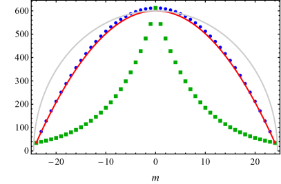
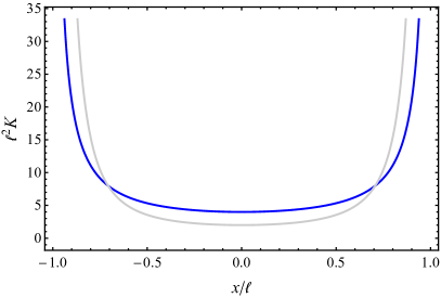
Figure 1: Left: couplings $J_{m+N/2-1}$ of the Lamé chain (7.3) with $k^{2}=1/2$ (blue dots), compared to those of the rainbow chain coinciding with the former at $m=0,\pm(N/2-1)$ (green squares), the continuum approximation $\ell^{2}J(m)$ in Eq. (7.5) for $N=50$ (red line), and the (scaled) Fermi velocity $\ell^{2}v_{F}(m)=\sqrt{\ell^{2}-m^{2}}$ (gray line) of a gas of free fermions trapped by the harmonic potential $V(x)=x^{2}$. Right: scalar curvature of the background space associated with the latter Lamé chain in the limit $N\to\infty$ (blue line) and with the gas of free fermions in a harmonic potential (gray line).

Note that, although $\kappa\to 1$ as $N\to\infty$ and therefore $J(x)\simeq 1-x^{2}/\ell^{2}$, we have not replaced $\kappa$ by $1$ in $J(x)$ since we need $\int_{0}^{\ell}J(x)^{-1}\mathrm{d}x$ to be convergent (see below). Note also that the limiting form of $J(x)$ is reminiscent of the (appropriately scaled) Fermi velocity $v_{F}(x)=\sqrt{1-x^{2}/\ell^{2}}$ of a gas of free fermions trapped in the harmonic potential $V(x)=x^{2}$ [17], the main difference being that in the latter case $\tilde{\ell}=\ell\pi/2$ is finite.

Substituting Eq. (7.5) into (7.4) we thus have

$$H\simeq\frac{\mathrm{i}\ell^{2}}{a}\int_{-\ell}^{\ell}J(x)\big{(}{\psi\vphantom{\psi^{\dagger}}}_{\mathrm{L}}^{\dagger}(x)\overset{\leftrightarrow}{\partial_{x}}{\psi\vphantom{\psi^{\dagger}}}_{\mathrm{L}}(x)-{\psi\vphantom{\psi^{\dagger}}}_{\mathrm{R}}^{\dagger}(x)\overset{\leftrightarrow}{\partial_{x}}{\psi\vphantom{\psi^{\dagger}}}_{\mathrm{R}}(x)\big{)}\mathrm{d}x\,,$$ (7.7)

with $J(x)$ given by Eq. (7.5). Using the boundary conditions [45]

$${\psi\vphantom{\psi^{\dagger}}}_{\mathrm{L}}(\pm\ell)=\pm\mathrm{i}{\psi\vphantom{\psi^{\dagger}}}_{\mathrm{R}}(\pm\ell)$$

and integrating by parts we obtain the equivalent expression

$$H\simeq\frac{2\mathrm{i}\ell^{2}}{a}\int_{-\ell}^{\ell}\Big{[} J(x)\big{(}{\psi\vphantom{\psi^{\dagger}}}_{\mathrm{L}}^{\dagger}(x)\partial_{x}{\psi\vphantom{\psi^{\dagger}}}_{\mathrm{L}}(x)-{\psi\vphantom{\psi^{\dagger}}}_{\mathrm{R}}^{\dagger}(x)\partial_{x}{\psi\vphantom{\psi^{\dagger}}}_{\mathrm{R}}(x)\big{)}$$ (7.8)

$$+\frac{J^{\prime}(x)}{2}\big{(}{\psi\vphantom{\psi^{\dagger}}}_{\mathrm{L}}^{\dagger}(x){\psi\vphantom{\psi^{\dagger}}}_{\mathrm{L}}(x)-{\psi\vphantom{\psi^{\dagger}}}_{\mathrm{R}}^{\dagger}(x){\psi\vphantom{\psi^{\dagger}}}_{\mathrm{R}}(x)\big{)}\big{]}\mathrm{d}x\,,$$ (7.9)

where $J^{\prime}:=\partial_{x}J$. The key observation in Ref. [16] is that the Lagrangian density associated with the Hamiltonian (7.8), namely (up to inessential multiplicative constants)

$${\mathcal{L}}={\psi\vphantom{\psi^{\dagger}}}_{\mathrm{L}}^{\dagger}\partial_{t}{\psi\vphantom{\psi^{\dagger}}}_{\mathrm{L}}+{\psi\vphantom{\psi^{\dagger}}}_{\mathrm{R}}^{\dagger}\partial_{t}{\psi\vphantom{\psi^{\dagger}}}_{\mathrm{R}}-J\big{(}{\psi\vphantom{\psi^{\dagger}}}_{\mathrm{L}}^{\dagger}\partial_{x}{\psi\vphantom{\psi^{\dagger}}}_{\mathrm{L}}-{\psi\vphantom{\psi^{\dagger}}}_{\mathrm{R}}^{\dagger}\partial_{x}{\psi\vphantom{\psi^{\dagger}}}_{\mathrm{R}}\big{)}-\frac{J^{\prime}}{2}\big{(}{\psi\vphantom{\psi^{\dagger}}}_{\mathrm{L}}^{\dagger}{\psi\vphantom{\psi^{\dagger}}}_{\mathrm{L}}-{\psi\vphantom{\psi^{\dagger}}}_{\mathrm{R}}^{\dagger}{\psi\vphantom{\psi^{\dagger}}}_{\mathrm{R}}\big{)}\,,$$ (7.10)

coincides with that of a free massless Dirac fermion in a curved background space with an appropriate metric. To see this in our case, and to compute the background metric, we recall the expression for the latter Lagrangian density:

$${\mathcal{L}}_{F}=e\,\overline{\Psi}\not{D}\Psi,\qquad\Psi:=\left({\psi\vphantom{\psi^{\dagger}}}_{\mathrm{L}}\atop{\psi\vphantom{\psi^{\dagger}}}_{\mathrm{R}}\right),\quad\overline{\Psi}:=\Psi^{\dagger}\gamma^{0}\,.$$

Here $e=\det(e_{\mu}^{a})$ is the determinant of the components of the dual $e^{a}_{\mu}$ of the zweibein $E_{a}^{\mu}=g^{\mu\nu}\eta_{ab}e^{b}_{\nu}$ (with $a,\mu\in\{0,1\}$) and $\not{D}=E^{\mu}_{a}\gamma^{a}D_{\mu}$, where summation over repeated indices is implied. The $\gamma$ matrices are $\gamma^{0}=\mathrm{i}\sigma^{x}$, $\gamma^{1}=\sigma^{y}$, and

$$D_{\mu}=\partial_{\mu}+\frac{1}{8}\,\omega^{ab}_{\mu}[\gamma_{a},\gamma_{b}]\,,$$

(with $\gamma_{a}=\eta_{ab}\gamma^{b}$ and $(\eta_{ab})=\mathop{\rm diag}\nolimits(-1,1)$), where $\omega^{ab}_{\mu}$ is the spin connection. The background metric $g_{\mu\nu}$ is then given by

$$g_{\mu\nu}=\eta_{ab}e^{a}_{\mu}e^{b}_{\nu}\,,$$

and the spin connection is determined by the metric through the equations

$$\omega^{ab}_{\mu}=e^{a}_{\nu}(\nabla_{\mu}E^{b})^{\nu}=e^{a}_{\nu}\big{(}\partial_{\mu}E^{b\nu}+\Gamma^{\nu}_{\lambda\mu}E^{b\lambda}\big{)}=-\omega^{ba}_{\mu}\,,$$ (7.11)

where $(\Gamma^{\nu}_{\lambda\mu})$ are the Christoffel symbols of the metric $g_{\mu\nu}$. If we assume that the zweibein is such that the matrix $(E^{\mu}_{a})$ (and hence $(e_{\mu}^{a})$) is diagonal, the Lagrangian density ${\mathcal{L}}_{F}$ reduces to

$${\mathcal{L}}_{F}=-\Psi^{\dagger}\bigg{(}e^{1}_{1}\partial_{t}+e^{0}_{0}\sigma^{z}\partial_{x}+\frac{1}{2}e^{1}_{1}\omega_{0}^{01}\sigma^{z}+\frac{1}{2}e^{0}_{0}\omega^{01}_{1}\bigg{)}\Psi\,.$$

Comparing with Eq. (7.10) we arrive at the system

$$e^{1}_{1}=-1,\quad e_{0}^{0}=J\,,\quad\omega_{0}^{01}=-J^{\prime},\quad\omega^{01}_{1}=0\,.$$ (7.12)

The metric is then given by

$$g_{00}=-(e_{0}^{0})^{2}=-J^{2}\,,\quad g_{11}=(e_{1}^{1})^{2}=1\,,\quad g_{01}=g_{10}=0\,,$$

and hence

$$\mathrm{d}s^{2}=-J^{2}(x)\mathrm{d}t^{2}+\mathrm{d}x^{2}\,.$$ (7.13)

The non-vanishing Christoffel symbols are

$$\Gamma^{0}_{01}=\Gamma^{0}_{10}=\partial_{x}\log J\,,\qquad\Gamma^{1}_{00}=\frac{1}{2}\partial_{x}J^{2}\,,$$

from which it easily follows that the last two equations in (7.12) are consistent with (7.11). The Ricci tensor of the background manifold is given by

$$R_{00}=JJ^{\prime\prime}\,,\quad R_{11}=-\frac{J^{\prime\prime}}{J}\,,\quad R_{01}=R_{10}=0,$$

and hence the scalar curvature reads

$$R=g^{\mu\nu}R_{\mu\nu}=-2\frac{J^{\prime\prime}}{J}\,.$$

Setting $\xi:=x/\ell$, $\kappa^{\prime 2}:=1-\kappa^{2}$, from Eq. (7.5) it easily follows that

$$R=\frac{2}{\ell^{2}}\,\frac{(1-\xi^{2})^{2}\big{(}2-\kappa^{\prime 2}-2(1-2\kappa^{\prime 2})\xi^{2}\big{)}+\kappa^{\prime 4}(3-2\xi^{2})\xi^{4}}{(1-\xi^{2})^{2}(1-\kappa^{2}\xi^{2})^{2}}\simeq\frac{4}{\ell^{2}-x^{2}}\,,$$

so that $R>0$ everywhere and $R\to\infty$ for $x\to\pm\ell$ (cf. Fig. 1 right). This is in sharp contrast with the analogous result for the rainbow chain studied in Refs. [44, 45, 16, 18], for which $J(x)=-\rme^{-h|x|}$ and consequently

$$R=4h\delta(x)-2h^{2}$$

is negative for $x\neq 0$ and singular at the origin. Again, the formula for the scalar curvature of the model under study resembles that of the free fermion gas trapped by a harmonic potential studied in Ref. [17], which in appropriate units is given by $R=2\ell^{2}(\ell^{2}-x^{2})^{-2}$ (cf. Fig. 1 right).

To obtain an asymptotic formula for the Rényi entanglement entropy $S_{A,\alpha}$ of the Lamé chain (7.3) with $k^{2}=1/2$, we pass to the conformally flat form of the metric (7.13)

$$\mathrm{d}s^{2}=J^{2}(-\mathrm{d}t^{2}+\mathrm{d}\tilde{x}^{2})\,.$$

through the change of variable

$$\tilde{x}:=\int_{0}^{x}J(y)^{-1}\mathrm{d}y\,.$$

Using again Eq. (7.5) we then obtain

$$\tilde{x}=\ell\mathop{\rm arcsn}\nolimits(x/\ell;\kappa)=\ell F(\arcsin(x/\ell);\kappa)\,,$$

where

$$F(\theta;\kappa):=\int_{0}^{\theta}\frac{\mathrm{d}\varphi}{1-\kappa^{2}\sin^{2}\varphi}$$

is the incomplete elliptic integral of the first kind. Hence $\tilde{x}\in[-\tilde{\ell},\tilde{\ell}\,]$, where the conformal length $\tilde{\ell}$ is given by

$$\tilde{\ell}=\ell F(\pi/2;\kappa)=K(\kappa)\ell=K\bigl{(}1-N^{-1}\bigr{)}\ell.$$

Note that as $N\to\infty$

$$\tilde{x}\simeq\ell\mathop{\rm arctanh}\nolimits(x/\ell)\,,$$ (7.14)

except near $x=\pm\ell$. On the other hand, the conformal length $\tilde{\ell}$ diverges logarithmically as $N\to\infty$; more precisely, we have [47]

$$K\bigl{(}1-N^{-1}\bigr{)}=\frac{1}{2}\log N+O(1)\,.$$

This behavior is again quite different from that of the rainbow chain, for which $\tilde{\ell}$ is finite (in fact, independent of $N$).

Since the Lagrangian density ${\mathcal{L}}$ associated with the continuum limit of the Lamé chain under study coincides with that of a massless Dirac fermion in the curved background with metric $\mathrm{d}s^{2}=J^{2}(-\mathrm{d}t^{2}+\mathrm{d}\tilde{x}^{2})$, the $N\to\infty$ behavior of the bipartite entanglement entropy $S_{A}$ of the former model can be analyzed by studying the Euclidean action corresponding to the Lagrangian density ${\mathcal{L}}_{F}=e\,\overline{\Psi}\not{D}\Psi$. The latter action can be written in complex isothermal coordinates as [17, 16]

$${\mathcal{S}}=\frac{1}{2\pi}\int J(x)\Big{(}{\psi\vphantom{\psi^{\dagger}}}_{\mathrm{L}}^{\dagger}\overset{\leftrightarrow}{\partial_{z}}{\psi\vphantom{\psi^{\dagger}}}_{\mathrm{L}}+{\psi\vphantom{\psi^{\dagger}}}_{\mathrm{R}}^{\dagger}\overset{\leftrightarrow}{\partial_{\bar{z}}}{\psi\vphantom{\psi^{\dagger}}}_{\mathrm{R}}\Big{)}\mathrm{d}z\wedge\mathrm{d}\bar{z}\,,$$

up to inessential constant factors. According to the result in Ref. [18], the Rényi entanglement entropy $S_{A,\alpha}$ of this model for a bipartition in which $A=[-l,-x]$ behaves as

$$S_{A,\alpha}=\frac{1}{12}\big{(}1+\alpha^{-1}\big{)}\log\biggl{(}\frac{2\tilde{\ell}}{\eta\pi}J(x)\cos\biggl{(}\frac{\pi\tilde{x}}{2\tilde{\ell}}\biggr{)}\biggr{)}\,,$$ (7.15)

where $\eta$ is an ultraviolet cutoff independent of $x$ and $\ell$. As explained above, from the latter formula we can deduce an asymptotic approximation for the Rényi entanglement entropy of the Lamé chain (7.3) with $k^{2}=1/2$ at half filling in the limit $N\to\infty$, for a bipartition with $A=\{0,\dots,L-1\}$. Indeed, defining $L_{\mathrm{rel}}:=L/N\in(0,1)$ we have

$$\frac{\ell-x}{2\ell}=L_{\mathrm{rel}}\enspace\Longleftrightarrow\enspace\frac{x}{l}=1-2L_{\mathrm{rel}}\,,$$

and therefore

$$J(x)\simeq 1-\frac{x^{2}}{\ell^{2}}=4L_{\mathrm{rel}}(1-L_{\mathrm{rel}})\,,$$

up to $O(N^{-1})$ terms. Using Eq. (7.14) for $\tilde{x}$ and setting $\ell=a(N-1)/2\simeq aN/2$ we obtain

$$S_{A,\alpha}\simeq\frac{1}{12}\big{(}1+\alpha^{-1}\big{)}\log\biggl{\{}\frac{4}{\pi}L_{\mathrm{rel}}(1-L_{\mathrm{rel}})NK\bigl{(}1-{\textstyle\frac{1}{N}}\bigr{)}\cos\biggl{(}\frac{\pi\mathop{\rm arctanh}\nolimits(1-2L_{\mathrm{rel}})}{2K\bigl{(}1-{\textstyle\frac{1}{N}}\bigr{)}}\biggr{)}\biggr{\}}+\gamma_{\alpha},$$ (7.16)

where $\gamma_{a}$ is a non-universal constant independent of $x$, $\ell$ and $N$. In fact, except for values of $L_{\mathrm{rel}}$ very close to $0$ or $1$ we can discard the $\cos$ term in the logarithm, since as $N\to\infty$ it is of order $(\log N)^{-2}$. Thus a simpler but still sufficiently accurate asymptotic formula for $S_{A}$ is

$$S_{A,\alpha}\simeq\frac{1}{12}\big{(}1+\alpha^{-1}\big{)}\log\biggl{[}\frac{4}{\pi}L_{\mathrm{rel}}(1-L_{\mathrm{rel}})NK\bigl{(}1-{\textstyle\frac{1}{N}}\bigr{)}\biggr{]}+\gamma_{\alpha},$$ (7.17)

or equivalently

$$S_{A,\alpha}\simeq\frac{1}{12}\big{(}1+\alpha^{-1}\big{)}\log\biggl{[}\frac{2}{\pi}L_{\mathrm{rel}}(1-L_{\mathrm{rel}})N\log N\biggr{]}+\tilde{\gamma}_{\alpha},$$ (7.18)

where $\tilde{\gamma}_{\alpha}$ is another constant independent of $x$, $\ell$ and $N$. Thus

$$S_{A,\alpha}\simeq\frac{1}{12}\big{(}1+\alpha^{-1}\big{)}\log N+O(\log\log N),$$

where the first term is characteristic of a critical system with central charge $c=1$, in the same universality class as a free fermion with open boundary conditions. Note, however, that the divergent part of $S_{A,\alpha}$,

$$S_{A,\alpha}\simeq\frac{1}{12}\big{(}1+\alpha^{-1}\big{)}\log(N\log N),$$

fundamentally differs from the well-known $\log N$ behavior found in the homogeneous XX chain and most one-dimensional critical models.

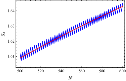
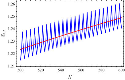
Figure 2: Rényi entanglement entropy of a single block of $\lfloor N/2\rfloor$ successive spins starting at the left end of the Lamé chain (7.3) with $k^{2}=1/2$ and $500\leqslant N\leqslant 600$ spins at half filling ($M=\lfloor N/2\rfloor$), for $\alpha=1$ (left) and $\alpha=2$ (right), compared to its CFT-based approximation (7.17) (continuous red line).

Using Eq. (7.1), we have numerically computed the Rényi entanglement entropy of a block of $L$ consecutive spins at the left end of the Lamé chain (7.3) with $k^{2}=1/2$ at half filling for several values of the Rényi parameter $\alpha$ and the relative block length $L_{\mathrm{rel}}=L/N$, with $N$ up to $600$ spins. To this end, it is necessary to compute the roots of the critical polynomial $P_{N}$ with very high accuracy, since in general the correlation matrix $C_{A}$ has a significant number of eigenvalues very close to $0$ or $1$. More precisely, we have found it necessary to work with $4N$ significant digits in the numerical computation of the roots of $P_{N}$ and the subsequent numerical diagonalization of the correlation matrix $C_{A}$. In general, the agreement of the numerical values of $S_{A,\alpha}$ thus obtained with the CFT asymptotic approximation (7.17) is quite good, particularly for $\alpha\leqslant 1$. For instance, in Fig. 2 we compare $S_{A,\alpha}$ with $\alpha=1,2$ to the latter CFT formula for $L_{\mathrm{rel}}=1/2$ and $N$ ranging from $500$ to $600$, where the non-universal parameter $\gamma_{\alpha}$ in Eq. (7.17) is estimated through a standard least squares fit of the data. It is apparent that the fit is excellent in both cases, the coefficient of variation (i.e., the root mean squared error divided by the mean, in percentage points) being equal to $0.164559$ for $\alpha=1$ and $0.670771$ for $\alpha=2$. Of course, what these comparisons actually test is whether $S_{A,\alpha}$ behaves as

$$S_{A,\alpha}\simeq\frac{1}{12}\big{(}1+\alpha^{-1}\big{)}\log\Bigl{(}NK\bigl{(}1-{\textstyle\frac{1}{N}}\bigr{)}\Bigr{)}+\text{const.},$$

not the specific dependence of the constant in the right-hand side with $L_{\mathrm{rel}}$ in Eq. (7.17). To ascertain the latter dependence, it suffices to note that if Eq. (7.17) holds the value of the parameter $\gamma_{\alpha}$ should not depend on $L_{\mathrm{rel}}$. In view of this observation, by way of example we have compared the value of $\gamma_{\alpha}$ in the range $0.1\leqslant\alpha\leqslant 5$ (at intervals of $0.05$) obtained fitting Eq. (7.17) to $S_{A,\alpha}$ with $500\leqslant N\leqslant 600$ for $L_{\mathrm{rel}}=1/4$ and $L_{\mathrm{rel}}=1/2$. As is apparent from Fig. 3 (left), both values differ by less than $10^{-2}$ for $\alpha\geqslant 0.25$ and by about $3\times 10^{-4}$ for $\alpha=5$, in excellent agreement with the $L_{\mathrm{rel}}$ dependence of $S_{A,\alpha}$ predicted by Eq. (7.17).

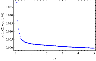
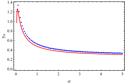
Figure 3: Left: difference between the parameter $\gamma_{\alpha}$ in Eq. (7.17) in the range $0.1\leqslant\alpha\leqslant 5$ (at intervals of $0.05$) for $L_{\mathrm{rel}}=1/2$ and $L_{\mathrm{rel}}=1/4$. In both cases, $\gamma_{\alpha}$ was computed by fitting $S_{A,\alpha}$ for $500\leqslant N\leqslant 600$ to Eq. (7.17). Right: parameter $\gamma_{\alpha}$ for the Lamé chain (7.3) with $k^{2}=1/2$ (blue dots) compared to the analogous quantity (7.19) for the uniform XX chain (red line).

Note, finally, that the numerical value of $\gamma_{\alpha}$ for the Lamé chain (7.3) with $k^{2}=1/2$ (for, e.g., $L_{\mathrm{rel}}=1/2$) is remarkably close to the exact value of its counterpart for the uniform XX chain, namely [5]

$$\gamma_{\alpha}=\frac{1}{2}\bigg{(}1+\frac{1}{\alpha}\bigg{)}\bigg{\{} \frac{1}{3}\log 2$$ (7.19)

$$+\int_{0}^{\infty}\bigg{[}\frac{\alpha}{1-\alpha^{2}}\,\Big{(}\alpha\mathop{\rm csch}\nolimits t-\mathop{\rm csch}\nolimits(t/\alpha)\Big{)}\mathop{\rm csch}\nolimits t-\frac{\rme^{-2t}}{6}\bigg{]}\,\frac{\mathrm{d}t}{t}\bigg{\}}$$

(cf. Fig. 3, right).

8 Conclusions and outlook

In this work we have established a connection between inhomogeneous XX spin chains (or free fermion systems) and quasi-exactly solvable models on the line constructed from the $\mathrm{sl}(2)$ algebra. Indeed, any such model generating a family of weakly orthogonal polynomials defines a corresponding XX chain, whose single-particle Hamiltonian is determined by the coefficients of the three-term recursion relation of the polynomial family. Moreover, two realizations of the same QES model equivalent under a projective transformation give rise to isomorphic chains. We have classified all QES models on the line giving rise to a weakly orthogonal polynomial system under projective transformations, finding six inequivalent families. Each of them generates a corresponding family of inhomogeneous XX chains, whose hopping amplitudes and on-site energies are simple algebraic functions of the chain sites. Although in some cases the hopping amplitudes of these chains coincide with those of the chains constructed from the classical Krawtchouk and dual Hahn polynomials in Ref. [22], their on-site energies differ. Thus the six types of XX chains introduced in this paper appear to be new. In particular, from these six new types one can construct two families of XX chains associated with different QES realizations of the well-known Lamé (finite gap) potential on the line.

From the polynomial family associated with an inhomogeneous XX chain it is straightforward to construct the correlation matrix of the corresponding free fermion system, whose eigenvalues yield its entanglement spectrum. In fact, this is one of the most efficient methods for computing the bipartite Rényi entanglement entropy of such models. We have used this method to analyze the entanglement entropy of one of the new Lamé chains, whose on-site energies vanish for a suitable value of the modulus of the elliptic function. This makes it possible to apply the CFT techniques in Ref. [18] to find an asymptotic formula for the entanglement entropy at half filling when the number of sites $N$ tends to infinity, which reproduces with great accuracy the numerical results. Interestingly, we show that although the leading behavior of the entropy is the characteristic one for a critical one-dimensional model with $c=1$, there is a correction proportional to $\log(\log N)$ which is unusual for this type of systems.

The above results suggest several possible lines for future research. To begin with, the CFT techniques applied in this work to approximate the entanglement entropy of one of the Lamé chains can also be used for the new chain associated with the well-known sextic QES potential, whose coefficients depend on a free parameter. In particular, it could be of interest to ascertain if in this case there is also a subleading $\log(\log N)$ correction to the leading $\log N$ behavior of the entanglement entropy. It would also be natural to explore whether the above field-theoretic techniques can be generalized to chains with non-vanishing on-site energies, and to arbitrary Fermi momentum. Of course, the bipartite entanglement entropy is only the simplest type of multipartite entropy one can consider, and in fact the asymptotic behavior of the multi-block Rényi entanglement entropies of the homogeneous XX model and similar free fermion systems have been widely studied (see, e.g., [6, 8, 9, 4, 10, 11]). A similar analysis for the Lamé chain introduced in this paper, or the new chain constructed from the sextic QES potential, would therefore be worth pursuing. Finally, another natural problem to investigate is whether any of the chains introduced in this work allows for perfect state transfer of spin excitations [49, 50, 19, 20]. Indeed, it is known that a necessary condition for this to happen is that both the hopping amplitude and on-site energy be symmetric about the center of the chain [21]. This is actually the case for many of the models introduced in this paper (for suitable values of the parameters), including the two families of Lamé chains.

Appendix A Classification of QES models admitting a weakly orthogonal polynomial family

In this appendix we provide the details of the classification in Section 6 of QES models on the line giving rise to a weakly orthogonal polynomial system (cf. Table 1). As explained in the latter section, these models are characterized by the fact that the quartic polynomial $P(z)$ in Eq. (5.7) vanishes at zero and infinity. Moreover, two such models are equivalent if their polynomials $P(z)$ and $\widetilde{P}(w)$ are related by a real projective transformation (6.2). We thus need to find all equivalence classes of real polynomials $P(z)$ of degree at most four vanishing at zero and infinity (and such that $P(z)$ is positive in some open interval), modulo real projective transformations (6.2). In fact, the classification in Section 6 follows easily by considering the root pattern of $P$ in the extended real line, which is invariant under projective transformations. Let us encode such a pattern by a list of positive integers $(m_{1},m_{2},\dots,m_{r})$, where $r\geqslant 2$ is the number of distinct real roots of $P$ and $m_{i}$ is the multiplicity of the $i$-th root. From the previous remarks it follows that the only allowed root patterns are

$$(2,1,1),\quad(2,2),\quad(3,1),\quad(1,1,1,1),\quad(1,1)\,.$$

We shall next see that the first root pattern gives rise to the first two canonical forms in Table 1, while each of the remaining patterns respectively yields the canonical forms $3$ to $6$. It shall be convenient to deal separately with the cases in which I) $P$ has at least one multiple real root, and II) all real roots of $P$ are simple.

I) $P$ has (at least) one multiple real root

This case corresponds to the first three root patterns above. Applying if necessary a projective transformation of the form $w=(z-a)^{-1}$, we can assume that $\infty$ is a multiple root of $P$, or equivalently that $\deg P\leqslant 2$. If $\deg P=1$ (corresponding to the root pattern $(3,1)$) then $P(z)=\nu z$ with $\nu\neq 0$, which is in turn mapped to $\widetilde{P}(w)=w$ (case 4 in Table 1) by the dilation $z=\nu w$. If $\deg P=2$, apart from the root at the origin $P$ must have an additional finite real root at $z=-a$, so that $P(z)=cz(z+a)$ with $c\neq 0$. The dilation $z=\lambda w$ then maps $P(z)$ to

$$\widetilde{P}(w)=\frac{c}{\lambda^{2}}\,\lambda w(\lambda w+a)=cw\bigg{(}w+\frac{a}{\lambda}\bigg{)}\,.$$

If $a=0$ we obtain the third canonical form in Table 1 (note that in this case $c=\nu$ must be positive, because otherwise $P$ would be nonpositive everywhere). If $a\neq 0$, setting $\lambda=\mathop{\rm sgn}\nolimits c\cdot a$ we have $\widetilde{P}(w)=|c|w(1+\mathop{\rm sgn}\nolimits c\cdot w)$, which yields the first canonical form for $c>0$ and the second one for $c<0$. This exhausts case I, since $\deg P=0$ if and only if $P=0$.

I) $P$ has no multiple real roots

There are two subcases to consider, depending on whether $P$ has four simple real roots or two real and two complex conjugate roots (including the root at infinity). In the first case (which corresponds to the root pattern $(1,1,1,1)$), up to a dilation we can write

$$P(z)=cz(z+1)(z+a)\,,$$

with $c\neq 0$ and $a\neq 0,1$. To begin with, we can assume that $c>0$, since the linear map $z=-w-1$ transforms $P(z)$ into $\widetilde{P}(w)=-cw(w+1)(w+1-a)$. Let us show, finally, that we can take $a\in(0,1)$. Indeed, if $a>0$ we apply the inversion $z=1/w$, which maps $P(z)$ into

$$\widetilde{P}(w)=cw^{3}\bigg{(}\frac{1}{w}+1\bigg{)}\bigg{(}\frac{1}{w}+a\bigg{)}=caw(w+1)\bigg{(}w+\frac{1}{a}\bigg{)}.$$

Since $ca>0$, and $1/a\in(0,1)$ if $a\notin(0,1)$, we see that $\tilde{P}$ coincides with the fifth canonical form in this case (with $a$ replaced by $1/a$). Finally, if $a<0$ we perform the projective transformation $z=-a(w+1)/w$, under which $P(z)$ is mapped to

$$\widetilde{P}(w)=\frac{c}{a^{2}}\,w^{4}(-a)\bigg{(}\frac{1}{w}+1\bigg{)}\bigg{(}1-a-\frac{a}{w}\bigg{)}\bigg{(}-\frac{a}{w}\bigg{)}=c(1-a)w(w+1)\bigg{(}w-\frac{a}{1-a}\bigg{)}.$$

Again, since $a<0$ we have $c(1-a)>0$ and

$$-\frac{a}{1-a}=\frac{|a|}{1+|a|}\in(0,1)\,,$$

so that $\widetilde{P}$ adopts the fifth canonical form in Table 1.

Consider, finally, the case in which $P$ has two complex conjugate and two real roots (necessarily at $0$ and $\infty$), corresponding to the last root pattern $(1,1)$. We can thus write

$$P(z)=cz(z^{2}+2az+b^{2})\,,$$

with $c\neq 0$ and $b>|a|$. We can obviously assume that $c>0$ (otherwise, apply the transformation $z=-w$). The dilation $z=bw$ then maps $P(z)$ into

$$\widetilde{P}(w)=\frac{c}{b^{2}}\,bw(b^{2}w^{2}+2abw+b^{2})=cbw\bigg{(}w^{2}+\frac{2a}{b}\,w+1\bigg{)}\,,$$

with $cb>0$ and $|a|/b<1$, which coincides with the sixth canonical form in Table 1.

References

References

- [1] Calabrese P and Cardy J, Entanglement entropy and quantum field theory, 2004 J. Stat. Mech.-Theory E. 2004 P06002(27)
- [2] Calabrese P and Cardy J, Entanglement entropy and conformal field theory, 2009 J. Phys. A: Math. Theor. 42 504005(36)
- [3] Jin B Q and Korepin V E, Quantum spin chain, Toeplitz determinants and the Fisher–Hartwig conjecture, 2004 J. Stat. Phys. 116 79
- [4] Calabrese P and Essler F H L, Universal corrections to scaling for block entanglement in spin- chains, 2010 J. Stat. Mech.-Theory E. 2010 P08029(28)
- [5] Fagotti M and Calabrese P, Universal parity effects in the entanglement entropy of chains with open boundary conditions, 2011 J. Stat. Mech.-Theory E. 2011 P01017(26)
- [6] Casini H and Huerta M, Remarks on the entanglement entropy for disconnected regions, 2009 J. High Energy Phys. 2009 048(18)
- [7] Calabrese P, Cardy J and Tonni E, Entanglement entropy of two disjoint intervals in conformal field theory, 2009 J. Stat. Mech.-Theory E. 2009 P11001(38)
- [8] Alba V, Tagliacozzo L and Calabrese P, Entanglement entropy of two disjoint blocks in critical Ising models, 2010 Phys. Rev. B 81 060411(R)(4)
- [9] Fagotti M and Calabrese P, Entanglement entropy of two disjoint blocks in chains, 2010 J. Stat. Mech.-Theory E. 2010 P04016(35)
- [10] Ares F, Esteve J G and Falceto F, Entanglement of several blocks in fermionic chains, 2014 Phys. Rev. A 90 062321(8)
- [11] Carrasco J A, Finkel F, González-López A and Tempesta P, A duality principle for the multi-block entanglement entropy of free fermion systems, 2017 Sci. Rep.-UK 7 11206(11)
- [12] Fisher M E and Hartwig R E, Toeplitz determinants: some applications, theorems and conjectures, 1968 Adv. Chem. Phys. 15 333
- [13] Basor E L, A localization theorem for Toeplitz determinants, 1979 Indiana Math. J. 28 975
- [14] Deift P, Its A and Krasovsky I, Asymptotics of Toeplitz, Hankel, and ToeplitzHankel determinants with Fisher–Hartwig singularities, 2011 Ann. Math. 174 1243
- [15] Vitagliano G, Riera A and Latorre J I, Volume-law scaling for the entanglement entropy in spin- chains, 2010 New J. Phys. 12 113049(16)
- [16] Rodríguez-Laguna J, Dubail J, Ramírez G, Calabrese P and Sierra G, More on the rainbow chain: entanglement, space-time geometry and thermal states, 2017 J. Phys. A: Math. Theor. 50 164001(18)
- [17] Dubail J, Stéphan J M, Viti J and Calabrese P, Conformal field theory for inhomogeneous one-dimensional quantum systems: the example of non-interacting Fermi gases, 2017 SciPost Phys. 2 002(21)
- [18] Tonni E, Rodríguez-Laguna J and Sierra G, Entanglement hamiltonian and entanglement contour in inhomogeneous 1D critical systems, 2018 J. Stat. Mech.-Theory E. 2018 043105(39)
- [19] Chakrabarti R and Van der Jeugt J, Quantum communication through a spin chain with interaction determined by a Jacobi matrix, 2010 J. Phys. A: Math. Theor. 43 085302(20)
- [20] Van der Jeugt J, Quantum communication and state transfer in spin chains, 2011 J. Phys. Conf. Ser. 284 012059(10)
- [21] Vinet L and Zhedanov A, How to construct spin chains with perfect state transfer, 2012 Phys. Rev. A 85 012323(7)
- [22] Crampé N, Nepomechie R I and Vinet L, Free-fermion entanglement and orthogonal polynomials, 2019 J. Stat. Mech.-Theory E. 2019 093101(17)
- [23] Turbiner A V, Quasi-exactly solvable problems and algebra, 1988 Commun. Math. Phys. 118 467
- [24] Shifman M A, New findings in quantum mechanics (partial algebraization of the spectral problem), 1989 Int. J. Mod. Phys. A 4 2897
- [25] Shifman M A and Turbiner A V, Quantal problems with partial algebraization of the spectrum, 1989 Commun. Math. Phys. 126 347
- [26] Ushveridze A G, Quasi-Exactly Solvable Models in Quantum Mechanics (Bristol: Institute of Physics Publishing) 1994
- [27] Bender C M and Dunne G V, Quasi-exactly solvable systems and orthogonal polynomials, 1996 J. Math. Phys. 37 6
- [28] Finkel F, González-López A and Rodríguez M A, Quasi-exactly solvable potentials on the line and orthogonal polynomials, 1996 J. Math. Phys. 37 3954
- [29] Arscott F M, Periodic Differential Equations (Oxford: Pergamon) 1964
- [30] Vidal G, Latorre J I, Rico E and Kitaev A, Entanglement in quantum critical phenomena, 2003 Phys. Rev. Lett. 90 227902(4)
- [31] Peschel I, Calculation of reduced density matrices from correlation functions, 2003 J. Phys. A: Math. Gen 36 L205
- [32] Chihara T S, An Introduction to Orthogonal Polynomials (New York: Gordon and Breach) 1978
- [33] González-López A, Kamran N and Olver P J, Normalizability of one-dimensional quasi-exactly solvable Schrödinger operators, 1993 Commun. Math. Phys. 153 117
- [34] González-López A, Kamran N and Olver P J, Quasi-exact solvability, 1994 Contemp. Math. 160 113
- [35] Krawtchouk M, Sur une généralisation des polynômes d’Hermite, 1929 C. R. Hebd. Seances Acad. Sci. 189 620
- [36] Hahn, Über Orthogonalpolynome, die -Differenzengleichungen genügen, 1949 Math. Nachr. 2 4
- [37] Alhassid Y, Gürsey F and Iachello F, Potential scattering, transfer matrix, and group theory, 1983 Phys. Rev. Lett. 50 873
- [38] Braibant S and Brihaye Y, Quasi-exactly-solvable system and sphaleron stability, 1993 J. Math. Phys. 34 2107
- [39] Greene P, Kofman L, Linde A and Starobinsky A, Structure of resonance in preheating after inflation, 1997 Phys. Rev. D 56 6175
- [40] Finkel F, González-López A, Maroto A L and Rodríguez M A, The Lamé equation in parametric resonance after inflation, 2000 Phys. Rev. D 62 103515(7)
- [41] Finkel F, González-López A and Rodríguez M A, A new algebraization of the Lamé equation, 2000 J. Phys. A: Math. Gen. 33 1519
- [42] Nielsen M A and Chuang I L, Quantum Computation and Quantum Information (Cambridge: Cambridge University Press), 10th Anniversary edition 2010
- [43] Katsura H, Sine-square deformation of solvable spin chains and conformal field theories, 2012 J. Phys. A: Math. Theor. 45 115003(17)
- [44] Ramírez G, Rodríguez-Laguna J and Sierra G, From conformal to volume law for the entanglement entropy in exponentially deformed critical spin chains, 2014 J. Stat. Mech.-Theory E. 2014 P10004(15)
- [45] Ramírez G, Rodríguez-Laguna J and Sierra G, Entanglement over the rainbow, 2015 J. Stat. Mech.-Theory E. 2015 06002(20)
- [46] Birrell N D and Davies P C W, Quantum Fields in Curved Space (Cambridge: Cambridge University Press) 1982
- [47] Olver F W J, Lozier D W, Boisvert R F and Clark C W, eds., NIST Handbook of Mathematical Functions (Cambridge University Press) 2010
- [48] Xavier J C, Alcaraz F C and Sierra G, Equipartition of the entanglement entropy, 2018 Phys. Rev. B 98 041106(R)(6)
- [49] Bose S, Quantum communication through spin chain dynamics: an introductory overview, 2007 Contemp. Phys. 48 13
- [50] Kay A, Perfect, efficient, state transfer and its application as a constructive tool, 2010 Int. J. Quantum Inf. 8 641