Distributed Linearly Separable Computation

Abstract

This paper formulates a distributed computation problem, where a master asks ${\mathsf{N}}$ distributed workers to compute a linearly separable function. The task function can be expressed as ${\mathsf{K}}_{\rm c}$ linear combinations of ${\mathsf{K}}$ messages, where each message is a function of one dataset. Our objective is to find the optimal tradeoff between the computation cost (number of uncoded datasets assigned to each worker) and the communication cost (number of symbols the master must download), such that from the answers of any ${\mathsf{N}}_{\rm r}$ out of ${\mathsf{N}}$ workers the master can recover the task function with high probability, where the coefficients of the ${\mathsf{K}}_{\rm c}$ linear combinations are uniformly i.i.d. over some large enough finite field. The formulated problem can be seen as a generalized version of some existing problems, such as distributed gradient coding and distributed linear transform.

In this paper, we consider the specific case where the computation cost is minimum, and propose novel achievability schemes and converse bounds for the optimal communication cost. Achievability and converse bounds coincide for some system parameters; when they do not match, we prove that the achievable distributed computing scheme is optimal under the constraint of a widely used ‘cyclic assignment’ scheme on the datasets. Our results also show that when ${\mathsf{K}}={\mathsf{N}}$, with the same communication cost as the optimal distributed gradient coding scheme proposed by Tandon et al. from which the master recovers one linear combination of ${\mathsf{K}}$ messages, our proposed scheme can let the master recover any additional ${\mathsf{N}}_{\rm r}-1$ independent linear combinations of messages with high probability.

I Introduction

Enabling large-scale computations for a large dimension of data, distributed computation systems such as MapReduce [1] and Spark [2] have received significant attention in recent years [3]. The distributed computation system divides a computational task into several subtasks, which are then assigned to some distributed workers. This reduces significantly the computing time by exploiting parallel computing procedures and thus enables handling of the computations over large-scale big data. However, while large scale distributed computing schemes have the potential for achieving unprecedented levels of accuracy and providing dramatic insights into complex phenomena, they also present some technical issues/bottlenecks. First, due to the presence of stragglers, a subset of workers may take excessively long time or fail to return their computed sub-tasks, which leads to an undesirable and unpredictable latency. Second, data and computed results should be communicated among the master who wants to compute the task, and the workers. If the communication bandwidth is limited, the communication cost becomes another bottleneck of the distributed computation system. In order to tackle these two bottlenecks, coding techniques were introduced to the distributed computing algorithms [4, 5, 6], with the purpose of increasing tolerance with respect to stragglers and reducing the master-workers communication cost. More precisely, for the first bottleneck, using ideas similar to Minimum Distance Separable (MDS) codes, the master can recover the task function from the answers of the fastest workers. For the second bottleneck, inspired by concepts from coded caching networks [7, 8], network coding techniques are used to save significant communication cost exchanged in the network.

In this paper, a master aims to compute a linearly separable function $f$ (such as linear MapReduce, Fourier Transform, convolution, etc.) on ${\mathsf{K}}$ datasets ($D_{1},\ldots,D_{{\mathsf{K}}}$), which can be written as

$$f(D_{1},\ldots,D_{{\mathsf{K}}})=g\big{(}f_{1}(D_{1}),\ldots,f_{{\mathsf{K}}}(D_{{\mathsf{K}}})\big{)}=g(W_{1},\ldots,W_{{\mathsf{K}}}).$$

$W_{k}=f_{k}(D_{k})$ for all $k\in\{1,\ldots,{\mathsf{K}}\}$ is the outcome of the component function $f_{k}(\cdot)$ applied to dataset $D_{k}$, and it is represented as a string of ${\mathsf{L}}$ symbols on an appropriate sufficiently large alphabet. For example, $W_{k}$ can be the intermediate value in linear MapReduce, an input signal in Fourier Transform, etc. We consider the case where $g(\cdot)$ is a linear map defined by ${\mathsf{K}}_{\rm c}$ linear combinations of the messages $W_{1},\ldots,W_{{\mathsf{K}}}$ with uniform i.i.d. coefficients over some large enough finite field; i.e., $g(W_{1},\ldots,W_{{\mathsf{K}}})$ can be seen as the matrix product ${\bf FW}$, where ${\bf F}$ is the coefficient matrix and ${\bf W}=[W_{1};\ldots;W_{{\mathsf{K}}}]$. We consider the distributed computation scenario, where $f(D_{1},\ldots,D_{{\mathsf{K}}})$ is computed in a distributed way by a group of ${\mathsf{N}}$ workers. Each dataset is assigned in an uncoded manner to a subset of workers and the number of datasets assigned to each worker cannot be larger than ${\mathsf{M}}$, which is referred to as the computation cost. Each worker should compute and send coded messages in terms of the datasets assigned to it, such that from the answers of any ${\mathsf{N}}_{\rm r}$ workers, the master can recover the task function with high probability. Given $({\mathsf{K}},{\mathsf{N}},{\mathsf{N}}_{\rm r},{\mathsf{K}}_{\rm c},{\mathsf{M}})$, we aim to find the optimal distributed computing scheme with data assignment, computing, and decoding phases, which leads to the minimum communication cost (i.e., the number of downloaded symbols by the master, normalized by ${\mathsf{L}}$).

We illustrate two examples of the formulated distributed scenario in Fig. 1 where ${\mathsf{K}}_{\rm c}=1$ and ${\mathsf{K}}_{\rm c}=2$, respectively. In both examples, we consider that ${\mathsf{K}}={\mathsf{N}}=3,{\mathsf{N}}_{\rm r}=2$, and that the number of datasets assigned to each worker is ${\mathsf{M}}=2$. Assume that the characteristic of $\mathbb{F}_{{\mathsf{q}}}$ is larger than $3$.

• When ${\mathsf{K}}_{\rm c}=1$, the considered problem (as shown in Fig. 1(a)) is equivalent to the distributed gradient coding problem in [9], which aims to compute the sum of gradients in learning tasks by distributed workers. The gradient coding proposed in [9] assigns the datasets to the workers in a cyclic way, where $D_{1}$ and $D_{2}$ are assigned to worker $1$, $D_{2}$ and $D_{3}$ are assigned to worker $2$, and $D_{3}$ and $D_{1}$ are assigned to worker $3$. Worker $1$ then computes and sends $\frac{W_{1}}{2}+W_{2}$. Worker $2$ sends $W_{2}-W_{3}$, and worker $3$ sends $\frac{W_{1}}{2}+W_{3}$. From any two sent coded messages, the master can recover the task function $W_{1}+W_{2}+W_{3}$. By the converse bound in [10], it can be proved that the gradient coding scheme [9] is optimal under the constraint of linear coding in terms of communication cost. Note that in our paper, from a novel converse bound, we prove the optimality of the gradient coding scheme [9] when ${\mathsf{K}}_{\rm c}=1$ by removing the constraint of linear coding.

• When ${\mathsf{K}}_{\rm c}=2$, besides $W_{1}+W_{2}+W_{3}$ we let the master also request another linear combination of the messages, e.g., $W_{1}+2W_{2}+3W_{3}$. Here, we propose a novel distributed computing scheme (as shown in Fig. 1(a)), which can compute this additional sum but with the same number of communicated symbols as the gradient coding scheme. With the same cyclic assignment, we let worker $1$ send $2W_{1}+W_{2}$, worker $2$ send $W_{2}+2W_{3}$, worker $3$ send $-W_{1}+W_{3}$. It can be checked that from any two sent coded messages, the master can recover both of the two requested sums. Hence, with the same communication cost as the gradient coding scheme [9], the proposed distributed computing scheme allows the master recover the two requested linear combinations.

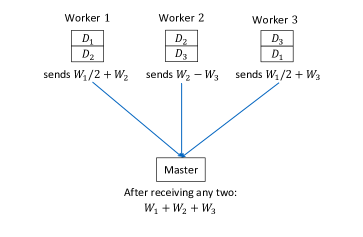
(a) ${\mathsf{K}}_{\rm c}=1$.

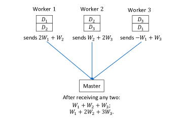
(b) ${\mathsf{K}}_{\rm c}=2$.

Figure 1: Distributed linearly separable computation with ${\mathsf{K}}={\mathsf{N}}=3$ and ${\mathsf{N}}_{\rm r}=2$. The number of datasets assigned to each worker is ${\mathsf{M}}=2$.

Since the seminal works on using coding techniques in distributed computing [4, 5, 6], different coded distributed computing schemes were proposed to compute various tasks in machine learning applications. The detailed comparison between the considered distributed linearly separable computation problem and each of the related existing works will be provided in Section II-B. In short,

• the distributed gradient coding problem considered in [9, 11, 12] is a special case of the considered problem in this paper with ${\mathsf{K}}_{\rm c}=1$ (i.e., the master requests one linear combination of the messages);

• the distributed linear transform problem considered in [13] is a special case of the considered problem in this paper where ${\mathsf{L}}=1$ (i.e., each message contains one symbol) and each worker sends one symbol;

• in the distributed matrix-vector multiplication problem considered in [14, 15, 16], the distributed matrix-matrix multiplication problem considered in [4, 17, 18, 19, 20, 21, 22, 23], and the distributed multivariate polynomial computation problem considered in [24], coded assignments are allowed, i.e., linear combinations of all input datasets can be assigned to each worker. Instead, in the considered problem the data assignment phase is uncoded, such that each worker can only compute functions of the datasets which are assigned to it.

Contributions

In this paper, we formulate the distributed linearly separable computation problem and consider the case where ${\mathsf{N}}$ divides ${\mathsf{K}}$ and the computation cost is minimum, i.e., ${\mathsf{M}}=\frac{{\mathsf{K}}}{{\mathsf{N}}}({\mathsf{N}}-{\mathsf{N}}_{\rm r}+1)$ by Lemma 1. Our main contributions on this case are as follows.

• We first propose an information theoretic converse bound on the minimum communication cost, inspired by the converse bound for the coded caching problem with uncoded cache placement [25, 26].

• With the cyclic assignment, widely used in the existing works on the distributed gradient coding problem such as [9, 11, 10], we propose a novel distributed computing scheme based on the linear space intersection and prove its decodability by the Schwartz-Zippel lemma [28, 29, 30].

• Compared to the proposed converse bound, the achievable scheme is proved to be optimal when ${\mathsf{N}}={\mathsf{K}}$, or ${\mathsf{K}}_{\rm c}\in\left\{1,\ldots,\left\lceil\frac{{\mathsf{K}}}{\binom{{\mathsf{N}}}{{\mathsf{N}}-{\mathsf{N}}_{\rm r}+1}}\right\rceil\right\}$, or ${\mathsf{K}}_{\rm c}\in\left\{\frac{{\mathsf{K}}}{{\mathsf{N}}}{\mathsf{N}}_{\rm r},\ldots,{\mathsf{K}}\right\}$. In addition, the proposed achievable scheme is proved to be optimal under the constraint of the cyclic assignment for all system parameters. The optimality results are listed in Table I at the top of the next page.

• By the derived optimality results, we obtain an interesting observation: when ${\mathsf{K}}={\mathsf{N}}$, for any ${\mathsf{K}}_{\rm c}\in\{1,\ldots,{\mathsf{N}}_{\rm r}\}$, the optimal communication cost is always ${\mathsf{N}}_{\rm r}$. Thus by taking the same communicatoin cost as the optimal gradient coding scheme in [9] for the distributed gradient coding problem (which is the case ${\mathsf{K}}_{\rm c}=1$ of our problem), with high probability our propose scheme can let the master recover any additional ${\mathsf{N}}_{\rm r}-1$ linear combinations with uniformly i.i.d. coefficients over $\mathbb{F}_{{\mathsf{q}}}$.

Moreover, for the case where ${\mathsf{N}}$ does not divide ${\mathsf{K}}$, the cyclic assignment cannot be directly used and we propose modified cyclic assignment and computing phases.

TABLE I: Optimality results for the distributed linearly separable computation problem where ${\mathsf{M}}=\frac{{\mathsf{K}}}{{\mathsf{N}}}({\mathsf{N}}-{\mathsf{N}}_{\rm r}+1)$ and ${\mathsf{N}}$ divides ${\mathsf{K}}$.

Constraint of system parameters	Optimality
${\mathsf{N}}={\mathsf{K}}$	optimal
${\mathsf{N}}\neq{\mathsf{K}}$, ${\mathsf{K}}_{\rm c}\in\left\{1,\ldots,\left\lceil\frac{{\mathsf{K}}}{\binom{{\mathsf{N}}}{{\mathsf{N}}-{\mathsf{N}}_{\rm r}+1}}\right\rceil\right\}$	optimal
${\mathsf{N}}\neq{\mathsf{K}}$, ${\mathsf{K}}_{\rm c}\in\left\{\frac{{\mathsf{K}}}{{\mathsf{N}}}{\mathsf{N}}_{\rm r},\ldots,{\mathsf{K}}\right\}$	optimal
${\mathsf{N}}\neq{\mathsf{K}}$, ${\mathsf{K}}_{\rm c}\in\left\{\left\lceil\frac{{\mathsf{K}}}{\binom{{\mathsf{N}}}{{\mathsf{N}}-{\mathsf{N}}_{\rm r}+1}}\right\rceil+1,\ldots,\frac{{\mathsf{K}}}{{\mathsf{N}}}{\mathsf{N}}_{\rm r}-1\right\}$	optimal under the cyclic assignment

Paper Organization

The rest of this paper is organized as follows. Section II formulates the distributed linearly separable computation problem and explains the differences from the existing distributed computation problem in the literature. Section III provides the main results in this paper. Section IV describes the proposed achievable distributed computing scheme. Section V discusses the extensions of the proposed results. Section VI concludes the paper and some of the proofs are given in the Appendices.

Notation Convention

Calligraphic symbols denote sets, bold symbols denote vectors and matrices, and sans-serif symbols denote system parameters. We use $|\cdot|$ to represent the cardinality of a set or the length of a vector; $[a:b]:=\left\{a,a+1,\ldots,b\right\}$, $(a:b]:=\{a+1,a+2,\ldots,b\}$, $[a:b):=\{a,a+1,\ldots,b-1\}$, $(a,b)=\{a+1,a+2,\ldots,b-1\}$ and $[n]:=[1:n]$; $\oplus$ represents bit-wise XOR; $\mathbb{E}[\cdot]$ represents the expectation value of a random variable; $a!=a\times(a-1)\times\ldots\times 1$ represents the factorial of $a$; $\mathbb{F}_{{\mathsf{q}}}$ represents a finite field with order ${\mathsf{q}}$; $\mathbf{M}^{\text{T}}$ and $\mathbf{M}^{-1}$ represent the transpose and the inverse of matrix $\mathbf{M}$, respectively; the matrix $[a;b]$ is written in a Matlab form, representing $[a,b]^{\text{T}}$; $\text{rank}(\mathbf{M})$ represents the rank of matrix $\mathbf{M}$; $\mathbf{I}_{n}$ represents the identity matrix with dimension $n\times n$; ${\bf 0}_{m\times n}$ represents the zero matrix with dimension $m\times n$; $(\mathbf{M})_{m\times n}$ represents that the dimension of matrix $\mathbf{M}$ is $m\times n$; $\mathbf{M}^{({\mathcal{S}})_{\rm r}}$ represents the sub-matrix of $\mathbf{M}$ which is composed of the rows of $\mathbf{M}$ with indices in ${\mathcal{S}}$ (here $\rm r$ represents ‘rows’); $\mathbf{M}^{({\mathcal{S}})_{\rm c}}$ represents the sub-matrix of $\mathbf{M}$ which is composed of the columns of $\mathbf{M}$ with indices in ${\mathcal{S}}$ (here $\rm c$ represents ‘columns’); $\text{det}(\mathbf{M})$ represents the determinant matrix $\mathbf{M}$; $\text{Mod}(b,a)$ represents the modulo operation on $b$ with integer divisor $a$ and in this paper we let $\text{Mod}(b,a)\in\{1,\ldots,a\}$ (i.e., we let $\text{Mod}(b,a)=a$ if $a$ divides $b$); we let $\binom{x}{y}=0$ if $x<0$ or $y<0$ or $x<y$. In this paper, for each set of integers ${\mathcal{S}}$, we sort the elements in ${\mathcal{S}}$ in an increasing order and denote the $i^{\text{th}}$ smallest element by ${\mathcal{S}}(i)$, i.e., ${\mathcal{S}}(1)<\ldots<{\mathcal{S}}(|{\mathcal{S}}|)$.

The main network parameters and notations are given in Table II at the top of the next page.

TABLE II: Main notations

Notations	Semantics
${\mathsf{K}}$	number of datasets
${\mathsf{N}}$	number of workers
${\mathsf{N}}_{\rm r}$	number of workers the master should wait for
${\mathcal{Z}}_{n}$	set of datasets assigned to worker $n$
${\mathsf{M}}$	computation cost (i.e., number of datasets assigned to each worker)
$X_{n}$	transmission of worker $n$
$T_{n}$	number of symbols in $X_{n}$
$X_{{\mathcal{A}}}$	$\{X_{n}:n\in{\mathcal{A}}\}$
${\mathsf{R}}$	communication cost
${\mathsf{R}}^{\star}$	minimum communication cost over all achievable computing schemes
${\mathsf{R}}^{\star}_{\text{cyc}}$	minimum communication cost over all achievable computing schemes with the cyclic assignment
$D_{n}$	the $n^{\text{th}}$ dataset
$W_{n}=f_{n}(D_{n})$	the $n^{\text{th}}$ message
${\mathsf{L}}$	number of symbols of each message
$g(W_{1},\ldots,W_{{\mathsf{N}}})={\bf F}[W_{1};\ldots;W_{{\mathsf{N}}}]$	task function (i.e., demanded linear combinations of messages)
${\mathsf{K}}_{\rm c}$	number of demanded linear combinations of messages (i.e., number of rows in ${\bf F}$)

II System Model

II-A Problem formulation

We formulate a $({\mathsf{K}},{\mathsf{N}},{\mathsf{N}}_{\rm r},{\mathsf{K}}_{\rm c},{\mathsf{M}})$ distributed linearly separable computation problem over the canonical master-worker distributed system, as illustrated in Fig. 1. The master wants to compute a function

$$f(D_{1},\ldots,D_{{\mathsf{K}}})$$

on ${\mathsf{K}}$ independent datasets $D_{1},\ldots,D_{{\mathsf{K}}}$. As the data sizes are large, we distribute the computing task to a group of ${\mathsf{N}}$ workers. For distributed computation to be possible, we assume the function is separable to some extent. As the simplest case, we assume the function is separable to each dataset,

$$f(D_{1},\ldots,D_{{\mathsf{K}}}) =g\big{(}f_{1}(D_{1}),\ldots,f_{{\mathsf{K}}}(D_{{\mathsf{K}}})\big{)}$$ (1a)

$$=g(W_{1},\ldots,W_{{\mathsf{K}}}),$$ (1b)

where we model $f_{k}(D_{k})$, $k\in[{\mathsf{K}}]$ as the $k$-th message $W_{k}$ and $f_{k}(\cdot)$ is an arbitrary function. We assume that the ${\mathsf{K}}$ messages are independent and that each message is composed of ${\mathsf{L}}$ uniformly i.i.d. symbols over a finite field $\mathbb{F}_{{\mathsf{q}}}$ for some large enough prime-power ${\mathsf{q}}$, where ${\mathsf{L}}$ is large enough such that any sub-message division is possible. We consider the simplest case of the function $g(\cdot)$, the linear mapping. So we can rewrite the task function as

$$g(W_{1},\ldots,W_{{\mathsf{K}}}) ={\bf F}\left[\begin{array}[]{c}W_{1}\\ \vdots\\ W_{{\mathsf{K}}}\end{array}\right]=\left[\begin{array}[]{c}F_{1}\\ \vdots\\ F_{{\mathsf{K}}_{\rm c}}\end{array}\right],$$ (2g)

where ${\bf F}$ is a matrix known by the master and the workers with dimension ${\mathsf{K}}_{\rm c}\times{\mathsf{K}}$, whose elements are uniformly i.i.d. over $\mathbb{F}_{{\mathsf{q}}}$. In other words, $g(W_{1},\ldots,W_{{\mathsf{K}}})$ contains ${\mathsf{K}}_{\rm c}$ linear combinations of the ${\mathsf{K}}$ messages, whose coefficients are uniformly i.i.d. over $\mathbb{F}_{{\mathsf{q}}}$. In this paper, we consider the case where ${\mathsf{K}}_{\rm c}\leq{\mathsf{K}}$. Note that each component function $f_{k}$ where $k\in[{\mathsf{K}}]$ is not restricted to be linear. We also assume that $\frac{{\mathsf{K}}}{{\mathsf{N}}}$ is an integer.

A computing scheme for our problem contains three phases, data assignment, computing, and decoding.

Data assignment phase

We assign each dataset $D_{k}$ where $k\in[{\mathsf{K}}]$ to a subset of ${\mathsf{N}}$ workers in an uncoded manner. The set of datasets assigned to worker $n\in[{\mathsf{N}}]$ is denoted by ${\mathcal{Z}}_{n}$, where ${\mathcal{Z}}_{n}\subseteq[{\mathsf{K}}]$. The assignment constraint is that

$$|{\mathcal{Z}}_{n}|\leq{\mathsf{M}},\ \forall n\in[{\mathsf{N}}],$$ (3)

where ${\mathsf{M}}$ represents the computation cost as explained in Footnote 2. The assignment function of worker $n$ is denoted by $\varphi_{n}$, where

$${\mathcal{Z}}_{n}=\varphi_{n}({\bf F})\subseteq[{\mathsf{K}}],$$ (4)

$$\varphi_{n}:[\mathbb{F}_{{\mathsf{q}}}]^{{\mathsf{K}}_{\rm c}{\mathsf{K}}}\to\Omega_{{\mathsf{M}}}({\mathsf{K}}),$$ (5)

and $\Omega_{{\mathsf{M}}}({\mathsf{K}})$ represents the set of all subsets of $[{\mathsf{K}}]$ of size not larger than ${\mathsf{M}}$. In other words, the data assignment phase is uncoded.

Computing phase

Each worker $n\in[{\mathsf{N}}]$ first computes the message $W_{k}=f_{k}(D_{k})$ for each $k\in{\mathcal{Z}}_{n}$. Then it computes

$$X_{n}=\psi_{n}(\{W_{k}:k\in{\mathcal{Z}}_{n}\},{\bf F})$$ (6)

where the encoding function $\psi_{n}$ is such that

$$\psi_{n} :[\mathbb{F}_{{\mathsf{q}}}]^{|{\mathcal{Z}}_{n}|{\mathsf{L}}}\times[\mathbb{F}_{{\mathsf{q}}}]^{{\mathsf{K}}_{\rm c}{\mathsf{K}}}\to[\mathbb{F}_{{\mathsf{q}}}]^{{\mathsf{T}}_{n}},$$ (7)

and ${\mathsf{T}}_{n}$ represents the length of $X_{n}$. Finally, worker $n$ sends $X_{n}$ to the master.

Decoding phase

The master only waits for the ${\mathsf{N}}_{\rm r}$ fastest workers’ answers to compute $g(W_{1},\ldots,W_{{\mathsf{K}}})$. Hence, the computing scheme can tolerate ${\mathsf{N}}-{\mathsf{N}}_{\rm r}$ stragglers. Since the master does not know a priori which workers are stragglers, the computing scheme should be designed so that from the answers of any ${\mathsf{N}}_{\rm r}$ workers, the master can recover $g(W_{1},\ldots,W_{{\mathsf{K}}})$. More precisely, for any subset of workers ${\mathcal{A}}\subseteq[{\mathsf{N}}]$ where $|{\mathcal{A}}|={\mathsf{N}}_{\rm r}$, with the definition

$$X_{{\mathcal{A}}}:=\{X_{n}:n\in{\mathcal{A}}\},$$ (8)

there exists a decoding function $\phi_{{\mathcal{A}}}$ such that

$$\hat{g}_{{\mathcal{A}}}=\phi_{{\mathcal{A}}}\big{(}X_{{\mathcal{A}}},{\bf F}\big{)},$$ (9)

where the decoding function $\phi_{{\mathcal{A}}}$ is such that

$$\phi_{{\mathcal{A}}}:[\mathbb{F}_{{\mathsf{q}}}]^{\sum_{n\in{\mathcal{A}}}{\mathsf{T}}_{n}}\times[\mathbb{F}_{{\mathsf{q}}}]^{{\mathsf{K}}_{\rm c}{\mathsf{K}}}\to[\mathbb{F}_{{\mathsf{q}}}]^{{\mathsf{K}}_{\rm c}{\mathsf{L}}}.$$ (10)

The worst-case probability of error is defined as

$$\varepsilon:=\max_{{\mathcal{A}}\subseteq[{\mathsf{N}}]:|{\mathcal{A}}|={\mathsf{N}}_{\rm r}}\Pr\{\hat{g}_{{\mathcal{A}}}\neq g(W_{1},\ldots,W_{{\mathsf{K}}})\}.$$ (11)

In addition, we denote the communication cost by,

$${\mathsf{R}}:=\max_{{\mathcal{A}}\subseteq[{\mathsf{N}}]:|{\mathcal{A}}|={\mathsf{N}}_{\rm r}}\frac{\sum_{n\in{\mathcal{A}}}{\mathsf{T}}_{n}}{{\mathsf{L}}},$$ (12)

representing the maximum normalized number of symbols downloaded by the master from any ${\mathsf{N}}_{\rm r}$ responding workers. The communication cost ${\mathsf{R}}$ is achievable if there exists a computing scheme with assignment, encoding, and decoding functions such that

$$\lim_{{\mathsf{q}}\to\infty}\varepsilon=0.$$ (13)

The minimum communication cost over all possible achievable computing schemes is denoted by ${\mathsf{R}}^{\star}$. Since the elements of ${\bf F}$ are uniformly i.i.d. over larger enough field, ${\bf F}$ is full-rank with high probability. By the simple cut-set bound, we have

$${\mathsf{R}}^{\star}\geq{\mathsf{K}}_{\rm c}.$$ (14)

The following lemma provides the minimum number of workers to whom each dataset should be assigned.

Lemma 1.

Each dataset must be assigned to at least ${\mathsf{N}}-{\mathsf{N}}_{\rm r}+1$ workers. $\square$

Proof:

Assume there exists one dataset (assumed to be $D_{k}$) assigned to only $\ell$ workers where $\ell<{\mathsf{N}}-{\mathsf{N}}_{\rm r}+1$. It can be seen that there exist at least ${\mathsf{N}}_{\rm r}$ workers which does not know $D_{k}$. Hence, the answers of these ${\mathsf{N}}_{\rm r}$ workers do not have any information of $W_{k}$, and thus cannot reconstruct $g(W_{1},\ldots,W_{{\mathsf{K}}})$ (recall that $g(W_{1},\ldots,W_{{\mathsf{K}}})$ depends on $W_{k}$ with high probability). ∎

In this paper, we consider the case where the computation cost is minimum, i.e., each dataset is assigned to ${\mathsf{N}}-{\mathsf{N}}_{\rm r}+1$ workers and

$${\mathsf{M}}=|{\mathcal{Z}}_{1}|=\cdots=|{\mathcal{Z}}_{{\mathsf{N}}}|=\frac{{\mathsf{K}}}{{\mathsf{N}}}({\mathsf{N}}-{\mathsf{N}}_{\rm r}+1).$$

The objective of this paper is to characterize the minimum communication cost for the case where the computation cost is minimum.

We then review the cyclic assignment, which was widely used in the existing works on the distributed gradient coding problem in [9] (which is a special case of the consdered problem as explained in the next subsection), such as the gradient coding schemes in [9, 12, 11, 10]. For each dataset $D_{k}$ where $k\in[{\mathsf{K}}]$, we assign $D_{k}$ to worker $j$, where $j\in\big{\{}\text{Mod}(k,{\mathsf{N}}),\text{Mod}(k-1,{\mathsf{N}}),\ldots,\text{Mod}(k-{\mathsf{N}}+{\mathsf{N}}_{\rm r},{\mathsf{N}})\big{\}}$. In other words, the set of datasets assigned to worker $n\in[{\mathsf{N}}]$ is

$${\mathcal{Z}}_{n} =\underset{p\in\left[0:\frac{{\mathsf{K}}}{{\mathsf{N}}}-1\right]}{\cup}\big{\{}\text{Mod}(n,{\mathsf{N}})+p{\mathsf{N}},\text{Mod}(n+1,{\mathsf{N}})+p{\mathsf{N}},\ldots,$$

$$\text{Mod}(n+{\mathsf{N}}-{\mathsf{N}}_{\rm r},{\mathsf{N}})+p{\mathsf{N}}\big{\}}$$ (15)

with cardinality $\frac{{\mathsf{K}}}{{\mathsf{N}}}({\mathsf{N}}-{\mathsf{N}}_{\rm r}+1)$. For example, if ${\mathsf{K}}={\mathsf{N}}=4$ and ${\mathsf{N}}_{\rm r}=3$, by the cyclic assignment with $p=0$ in (15), we assign

$$D_{1},D_{2},D_{3}\ \text{to woker 1};$$

$$D_{2},D_{3},D_{4}\ \text{to woker 2};$$

$$D_{3},D_{4},D_{1}\ \text{to woker 3};$$

$$D_{4},D_{1},D_{2}\ \text{to woker 4}.$$

The minimum communication cost under the cyclic assignment in (15) is denoted by ${\mathsf{R}}^{\star}_{\rm cyc}$.

II-B Connection to existing problems

Distributed gradient coding

When $f_{k}(D_{k})$, $k\in[{\mathsf{K}}]$, represents the partial gradient vector of the loss at the current estimate of the dataset $D_{k}$ and ${\bf F}=[1,\ldots,1]$, we have

$$f(D_{1},\ldots,D_{{\mathsf{K}}})=f_{1}(D_{1})+\cdots+f_{{\mathsf{K}}}(D_{{\mathsf{K}}}),$$ (16)

representing the gradient of a generic loss function. In this case, our problem reduces to the distributed gradient coding problem in [9]. Hence, the distributed gradient coding problem in [9] is a special case of the distributed linearly separable computation problem with ${\mathsf{K}}_{\rm c}=1$. For the case where the computation cost is minimum, based on the cyclic assignment in (15) and a random code construction, the authors in [9] proposed a gradient coding scheme which lets each worker compute and send one linear combination of the messages related to its assigned datasets, while the achieved communication cost of this scheme is optimal under the constraint of linear coding [10]. Instead of random code construction, a deterministic code construction was proposed in [11]. The authors in [12] improved the decoding delay/complexity by using Reed–Solomon codes.

The authors in [10] characterized the optimal tradeoff between the computation cost and communication cost for the distributed gradient coding problem. A distributed computing scheme achieving the same optimal computation-communication costs tradeoff as in [10] but with lower decoding complexity, was recently proposed in [31].

Some other extensions on the distributed gradient coding problem in [9] were also considered in the literature. For instance, the authors in [32] extended the gradient coding strategy to a tree-topology where the workers are located, and a fixed fraction of children nodes per parent node may be straggler. The case where the number of stragglers is not given in prior was considered in [33]. In [34], each worker sends multiple linear combinations such that the master does not always need to wait for the answers of ${\mathsf{N}}_{\rm r}$ workers (i.e., from some ‘good’ subset of workers with the cardinality less than ${\mathsf{N}}_{\rm r}$, the master can recover the task function). It can be seen that these extended models are different from the considered problem in this paper.

Distributed linear transform

The distributed linear transform problem in [13] aims to compute the linear transform ${\bf A}{\mathbf{x}}$ where ${\mathbf{x}}$ is the input vector and ${\bf A}$ is a given matrix with dimension ${\mathsf{K}}_{\rm c}\times{\mathsf{K}}$. We should design a coding vector ${\mathbf{c}}_{n}$ for each worker $n\in[{\mathsf{N}}]$ (which then computes ${\mathbf{c}}_{n}{\mathbf{x}}$) such that from the computation results of any ${\mathsf{N}}_{\rm r}$ workers we can reconstruct ${\bf A}{\mathbf{x}}$. Meanwhile, in order to have low computation cost, each coding vector should be sparse and the number of its non-zero elements should be no more than ${\mathsf{M}}$, where ${\mathsf{M}}$ should be minimized. Hence, the distributed linear transform problem in [13] can be seen a special case of the distributed linearly separable computation problem with ${\mathsf{T}}_{n}={\mathsf{L}}=1$ for each $n\in[{\mathsf{N}}]$ (recall that ${\mathsf{T}}_{n}$ represents the number of symbols transmitted by worker $n$). In other words, in this paper we consider the case where the computation cost is minimum and search for the minimum communication cost, while the authors in [13] considered the case where ${\mathsf{L}}=1$ and the communication cost is minimum, and searched for the minimum computation cost. A computing scheme was proposed in [13] which needs ${\mathsf{M}}=\frac{{\mathsf{K}}}{{\mathsf{N}}}({\mathsf{N}}-{\mathsf{N}}_{\rm r}+{\mathsf{K}}_{\rm c})$. The authors in [35] further improved the distributed linear transform scheme in [13] by proposing a computing scheme to let each worker $n\in[{\mathsf{N}}]$ only access ${\mathsf{M}}^{\prime}_{n}$ elements in ${\mathbf{x}}$, where ${\mathsf{K}}({\mathsf{N}}-{\mathsf{N}}_{\rm r}+{\mathsf{K}}_{\rm c})-{\mathsf{N}}{\mathsf{N}}_{\rm r}<\sum_{n\in[{\mathsf{N}}]}{\mathsf{M}}^{\prime}_{n}<{\mathsf{N}}\frac{{\mathsf{K}}}{{\mathsf{N}}}({\mathsf{N}}-{\mathsf{N}}_{\rm r}+{\mathsf{K}}_{\rm c})$.

The authors in [36] considered another distributed linear transform problem with a different sparsity constraint compared to [13]. The distributed linear transform problem in [36] can be seen as a special case of the distributed linearly separable computation problem with ${\mathsf{T}}_{n}={\mathsf{L}}=1$ and ${\mathsf{K}}_{\rm c}={\mathsf{K}}$.

Distributed matrix-vector and matrix-matrix multiplications

Distributed computing techniques against stragglers were also used to compute matrix-vector multiplication as ${\bf Ab}$ [14, 15, 16] and matrix-matrix multiplication as ${\bf AB}$ [4, 17, 18, 19, 20, 21, 22, 23]. The general technique is to partition each input matrix into sub-matrices and assign some linear combinations of all sub-matrices (from MDS codes, polynomial codes, etc.) to the workers without considering the sparsity of the coding vectors/matrices. Thus, the assignment phase is coded.

Distributed multivariate polynomial computation

Similar difference as above also appears between the considered distributed linearly separable computation problem and the distributed multivariate polynomial computation problem in [24]. It was shown in [24] that the gradient descent can be computed distributedly by using a coding scheme based on the Lagrange polynomial. However, the assignment phase of the Lagrange distributed computing scheme in [24] is coded.

In summary, compared to the distributed computing schemes with coded assignment phase, the main challenge of designing computing schemes with uncoded assignment phase is that besides the decodability constraint, we should additionally guarantee that in the transmitted linear combination(s) by each worker, the coefficients of the unassigned elements are $0$.

III Main Results

We first propose a converse bound on the minimum communication cost in the following theorem, which will be proved in Appendix A inspired by the converse bound for the coded caching problem with uncoded cache placement [25, 26].

Theorem 1 (Converse).

For the $({\mathsf{K}},{\mathsf{N}},{\mathsf{N}}_{\rm r},{\mathsf{K}}_{\rm c},{\mathsf{M}})$ distributed linearly separable computation problem with ${\mathsf{M}}=\frac{{\mathsf{K}}}{{\mathsf{N}}}({\mathsf{N}}-{\mathsf{N}}_{\rm r}+1)$,

• when ${\mathsf{K}}_{\rm c}\in\left[\left\lceil\frac{{\mathsf{K}}}{\binom{{\mathsf{N}}}{{\mathsf{N}}-{\mathsf{N}}_{\rm r}+1}}\right\rceil\right]$, we have

  $${\mathsf{R}}^{\star}\geq{\mathsf{N}}_{\rm r}{\mathsf{K}}_{\rm c}.$$ (17a)

• when ${\mathsf{K}}_{\rm c}\in\left(\left\lceil\frac{{\mathsf{K}}}{\binom{{\mathsf{N}}}{{\mathsf{N}}-{\mathsf{N}}_{\rm r}+1}}\right\rceil:{\mathsf{K}}\right]$, we have

  $${\mathsf{R}}^{\star}\geq\max\left\{{\mathsf{N}}_{\rm r}\left\lceil\frac{{\mathsf{K}}}{\binom{{\mathsf{N}}}{{\mathsf{N}}-{\mathsf{N}}_{\rm r}+1}}\right\rceil,{\mathsf{K}}_{\rm c}\right\}.$$ (17b)

$\square$

For the case with ${\mathsf{K}}_{\rm c}=1$ and ${\mathsf{M}}=\frac{{\mathsf{K}}}{{\mathsf{N}}}({\mathsf{N}}-{\mathsf{N}}_{\rm r}+1)$ which reduces to the distributed gradient coding problem in [9], from Theorem 1 and the gradient coding scheme in [9] (each worker sends one linear combination of the assigned messages), we can directly prove the following corollary.

Corollary 1.

For the $({\mathsf{K}},{\mathsf{N}},{\mathsf{N}}_{\rm r},{\mathsf{K}}_{\rm c},{\mathsf{M}})$ distributed linearly separable computation problem with ${\mathsf{M}}=\frac{{\mathsf{K}}}{{\mathsf{N}}}({\mathsf{N}}-{\mathsf{N}}_{\rm r}+1)$ and ${\mathsf{K}}_{\rm c}=1$, we have

$${\mathsf{R}}^{\star}={\mathsf{N}}_{\rm r}.$$ (18)

$\square$

Note that the optimality of the gradient coding scheme in [9] for the distributed gradient coding problem was proved in [10], but under the constraint that the encoding functions in (7) are linear. In Corollary 1, we remove this constraint.

With the cyclic assignment in Section II-A, we then propose a novel achievable distributed computing scheme whose detailed proof could be found in Section IV.

Theorem 2 (Proposed distributed computing scheme).

For the $({\mathsf{K}},{\mathsf{N}},{\mathsf{N}}_{\rm r},{\mathsf{K}}_{\rm c},{\mathsf{M}})$ distributed linearly separable computation problem with ${\mathsf{M}}=\frac{{\mathsf{K}}}{{\mathsf{N}}}({\mathsf{N}}-{\mathsf{N}}_{\rm r}+1)$, the communication cost ${\mathsf{R}}_{{\rm ach}}$ is achievable, where

• when ${\mathsf{K}}_{\rm c}\in\left[1:\frac{{\mathsf{K}}}{{\mathsf{N}}}\right)$,

  $${\mathsf{R}}_{{\rm ach}}={\mathsf{N}}_{\rm r}{\mathsf{K}}_{\rm c};$$ (19a)

• when ${\mathsf{K}}_{\rm c}\in\left[\frac{{\mathsf{K}}}{{\mathsf{N}}}:\frac{{\mathsf{K}}}{{\mathsf{N}}}{\mathsf{N}}_{\rm r}\right]$,

  $${\mathsf{R}}_{{\rm ach}}=\frac{{\mathsf{K}}}{{\mathsf{N}}}{\mathsf{N}}_{\rm r};$$ (19b)

• when ${\mathsf{K}}_{\rm c}\in\left(\frac{{\mathsf{K}}}{{\mathsf{N}}}{\mathsf{N}}_{\rm r}:{\mathsf{K}}\right]$,

  $${\mathsf{R}}_{{\rm ach}}={\mathsf{K}}_{\rm c}.$$ (19c)

$\square$

In Theorem 2, we consider three regimes with respect to the value of ${\mathsf{K}}_{\rm c}$ and the main ingredients are as follows.

1. ${\mathsf{K}}_{\rm c}\in\left[1:\frac{{\mathsf{K}}}{{\mathsf{N}}}\right)$. By some linear transformations on the request matrix ${\bf F}$, we treat the considered problem as ${\mathsf{K}}_{\rm c}$ sub-problems in each of which the master requests one linear combination of messages. Thus by using the coding scheme in Corollary 1 for each sub-problem, we can let the master recover the general task function.

2. ${\mathsf{K}}_{\rm c}\in\left[\frac{{\mathsf{K}}}{{\mathsf{N}}}:\frac{{\mathsf{K}}}{{\mathsf{N}}}{\mathsf{N}}_{\rm r}\right]$. This is the most interesting case, where we propose a computing scheme based on the linear space intersection (see Remark 2 for further explanations), with the communication cost equal to the case where ${\mathsf{K}}_{\rm c}=\frac{{\mathsf{K}}}{{\mathsf{N}}}$. We generate $\frac{{\mathsf{K}}}{{\mathsf{N}}}{\mathsf{N}}_{\rm r}-{\mathsf{K}}_{\rm c}$ virtually requested linear combinations of messages such that the master totally recover $\frac{{\mathsf{K}}}{{\mathsf{N}}}{\mathsf{N}}_{\rm r}$ effective linear combinations of messages from the responses of any ${\mathsf{N}}_{\rm r}$ workers. Each worker transmits $\frac{{\mathsf{K}}}{{\mathsf{N}}}$ linear combinations of messages which lie in the intersection of the linear spaces of its known messages and the effective demanded linear combinations. From a highly non-trivial proof based on the Schwartz-Zippel lemma [28, 29, 30], where the main challenge is to prove that the multivariate polynomials are generally non-zero (see Appendix D), we show that the responses of any ${\mathsf{N}}_{\rm r}$ workers are linearly independent with high probability, and thus are able to reconstruct the effective demanded linear combinations.

3. ${\mathsf{K}}_{\rm c}\in\left(\frac{{\mathsf{K}}}{{\mathsf{N}}}{\mathsf{N}}_{\rm r}:{\mathsf{K}}\right]$. To recover ${\mathsf{K}}_{\rm c}$ linear combinations of the ${\mathsf{K}}$ messages, we propose a computing scheme to let the master totally receive ${\mathsf{K}}_{\rm c}$ coded messages with ${\mathsf{L}}$ symbols each, i.e., ${\mathsf{R}}^{\star}={\mathsf{K}}_{\rm c}$ is achieved.

Remark 1.

Note that, when the operations are on the field of real numbers, the proposed computing scheme in Theorem 2 can work with high probability if each element in ${\bf F}$ is uniformly i.i.d. over a large enough finite set of real numbers or over an interval of real numbers. $\square$

By comparing the proposed converse bound in Theorem 1 and the achievable scheme in Theorem 2, we can directly derive the following optimality results.

Theorem 3 (Optimality).

For the $({\mathsf{K}},{\mathsf{N}},{\mathsf{N}}_{\rm r},{\mathsf{K}}_{\rm c},{\mathsf{M}})$ distributed linearly separable computation problem with ${\mathsf{M}}=\frac{{\mathsf{K}}}{{\mathsf{N}}}({\mathsf{N}}-{\mathsf{N}}_{\rm r}+1)$,

• when ${\mathsf{K}}={\mathsf{N}}$, we have

  $${\mathsf{R}}^{\star}=\begin{cases}{\mathsf{N}}_{\rm r},&\text{ if }{\mathsf{K}}_{\rm c}\in[{\mathsf{N}}_{\rm r}];\\ {\mathsf{K}}_{\rm c},&\text{ if }{\mathsf{K}}_{\rm c}\in({\mathsf{N}}_{\rm r}:{\mathsf{K}}];\end{cases}$$ (20a)

• when ${\mathsf{K}}_{\rm c}\in\left[\left\lceil\frac{{\mathsf{K}}}{\binom{{\mathsf{N}}}{{\mathsf{N}}-{\mathsf{N}}_{\rm r}+1}}\right\rceil\right]$, we have

  $${\mathsf{R}}^{\star}={\mathsf{N}}_{\rm r}{\mathsf{K}}_{\rm c};$$ (20b)

• when ${\mathsf{K}}_{\rm c}\in\left[\frac{{\mathsf{K}}}{{\mathsf{N}}}{\mathsf{N}}_{\rm r}:{\mathsf{K}}\right]$, we have

  $${\mathsf{R}}^{\star}={\mathsf{K}}_{\rm c}.$$ (20c)

$\square$

From Theorem 3, it can be seen that when ${\mathsf{K}}={\mathsf{N}}$ and ${\mathsf{K}}_{\rm c}\in[{\mathsf{N}}_{\rm r}]$, the optimal communication cost is always ${\mathsf{N}}_{\rm r}$ (i.e., each worker sends one linear combination of the messages from its assigned datasets). Thus we prove that with the same communication cost as the optimal gradient coding scheme in [9] for the distributed gradient coding problem (from which the master recovers $W_{1}+\cdots W_{{\mathsf{K}}}$), our propose scheme can let the master recover any additional ${\mathsf{N}}_{\rm r}-1$ linear combinations of the ${\mathsf{K}}$ messages whose coefficients are uniformly i.i.d. over $\mathbb{F}_{{\mathsf{q}}}$ with high probability.

In general, the minimum communication cost in the regime where ${\mathsf{K}}_{\rm c}\in\left(\left\lceil\frac{{\mathsf{K}}}{\binom{{\mathsf{N}}}{{\mathsf{N}}-{\mathsf{N}}_{\rm r}+1}}\right\rceil:\frac{{\mathsf{K}}}{{\mathsf{N}}}{\mathsf{N}}_{\rm r}\right)$ is still open. The following theorem claims that the proposed achievable scheme is optimal under the constraint of the cyclic assignment in [9], whose proof is in Appendix B.

Theorem 4 (Optimality under the cyclic assignment in [9]).

For the $({\mathsf{K}},{\mathsf{N}},{\mathsf{N}}_{\rm r},{\mathsf{K}}_{\rm c},{\mathsf{M}})$ distributed linearly separable computation problem with ${\mathsf{M}}=\frac{{\mathsf{K}}}{{\mathsf{N}}}({\mathsf{N}}-{\mathsf{N}}_{\rm r}+1)$, the minimum communication cost under the cyclic assignment is

$${\mathsf{R}}^{\star}_{\rm cyc}={\mathsf{R}}_{{\rm ach}},$$ (21)

where ${\mathsf{R}}_{{\rm ach}}$ is given in (• ‣ 2). $\square$

IV Achievable Distributed Computing Scheme

In this section, we introduce the proposed distributed computing scheme with the cyclic assignment in [9]. As shown in Theorem 2, we divide the range of ${\mathsf{K}}_{\rm c}$ (which is $[{\mathsf{K}}]$) into three regimes, and present the corresponding scheme in the order, ${\mathsf{K}}_{\rm c}\in\left[\frac{{\mathsf{K}}}{{\mathsf{N}}}:\frac{{\mathsf{K}}}{{\mathsf{N}}}{\mathsf{N}}_{\rm r}\right]$, ${\mathsf{K}}_{\rm c}\in\left[1:\frac{{\mathsf{K}}}{{\mathsf{N}}}\right)$, and ${\mathsf{K}}_{\rm c}\in\left(\frac{{\mathsf{K}}}{{\mathsf{N}}}{\mathsf{N}}_{\rm r}:{\mathsf{K}}\right]$.

IV-A ${\mathsf{K}}_{\rm c}\in\left[\frac{{\mathsf{K}}}{{\mathsf{N}}}:\frac{{\mathsf{K}}}{{\mathsf{N}}}{\mathsf{N}}_{\rm r}\right]$

We first illustrate the main idea in the following example.

Example 1 (${\mathsf{N}}=3,{\mathsf{K}}=6,{\mathsf{K}}_{\rm c}=4,{\mathsf{N}}_{\rm r}=2$, ${\mathsf{M}}=4$).

In this example, it can be seen that ${\mathsf{K}}_{\rm c}=\frac{{\mathsf{K}}}{{\mathsf{N}}}{\mathsf{N}}_{\rm r}$. For the sake of simplicity, in the rest of this paper while illustrating the proposed schemes through examples, we assume that the field is a large enough prime field. It will be proved that in general this assumption is not necessary in our proposed schemes where we only need the field size ${\mathsf{q}}$ is large enough. Assume that the task function is

$$f(D_{1},\ldots,D_{6}) =\left[\begin{array}[]{c}F_{1}\\ F_{2}\\ F_{3}\\ F_{4}\\ \end{array}\right]={\bf F}\left[\begin{array}[]{c}W_{1}\\ W_{2}\\ W_{3}\\ W_{4}\\ W_{5}\\ W_{6}\end{array}\right]$$

$$=\left[\begin{array}[]{c}1,1,1,1,1,1\\ 1,2,3,4,5,6\\ 1,0,2,3,5,4\\ 1,2,1,4,4,0\\ \end{array}\right]\left[\begin{array}[]{c}W_{1}\\ W_{2}\\ W_{3}\\ W_{4}\\ W_{5}\\ W_{6}\end{array}\right].$$

Data assignment phase

By the cyclic assignment described in Section II-A, we assign that

$$\begin{array}[]{rl|c|c|c|}\cline{3-3}\cr\cline{4-4}\cr\cline{5-5}\cr&&\rule{0.0pt}{11.99998pt}\mbox{Worker 1}&\rule{0.0pt}{11.99998pt}\mbox{Worker 2}&\rule{0.0pt}{11.99998pt}\mbox{Worker 3}\\ \cline{3-3}\cr\cline{4-4}\cr\cline{5-5}\cr&&D_{1}&D_{2}&D_{1}\\ &&D_{2}&D_{3}&D_{3}\\ \cdashline{3-3}\cdashline{4-4}\cdashline{5-5}&&D_{4}&D_{5}&D_{4}\\ &&D_{5}&D_{6}&D_{6}\\ \cline{3-3}\cr\cline{4-4}\cr\cline{5-5}\cr\end{array}$$

Computing phase

We first focus on worker $1$, who first computes $W_{1}$, $W_{2}$, $W_{4}$, and $W_{5}$ based on its assigned datasets. In other words, $W_{i}$ where $i\in\{3,6\}$ cannot be computed by worker $1$. We retrieve the $i^{\text{th}}$ column of ${\bf F}$ where $i\in\{3,6\}$, to obtain

$${\bf F}^{(\{3,6\})_{\rm c}}=\left[\begin{array}[]{c}1,1\\ 3,6\\ 2,4\\ 1,0\\ \end{array}\right].$$ (26)

We then search for a vector basis for the left-side null space of ${\bf F}^{(\{3,6\})_{\rm c}}$. Note that ${\bf F}^{(\{3,6\})_{\rm c}}$ is a full-rank matrix with dimension $4\times 2$. Hence, a vector basis for its left-side null space contains $4-2=2$ linearly independent vectors with dimension $1\times 4$, where the product of each vector and ${\bf F}^{(\{3,6\})_{\rm c}}$ is ${\bf 0}_{1\times 2}$ (i.e., the zero matrix with dimension $1\times 2$). A possible vector basis could be the set of vectors $(-6,1,0,3)$ and $(0,-2,3,0)$. It can be seen that

$$\negmedspace\negmedspace-6F_{1}+1F_{2}+0F_{3}+3F_{4}\negmedspace=\negmedspace-2W_{1}+2W_{2}+10W_{4}+11W_{5},$$ (27a)

$$0F_{1}-2F_{2}+3F_{3}+0F_{4}=W_{1}-4W_{2}+W_{4}+5W_{5},$$ (27b)

both of which are independent of $W_{3}$ and $W_{6}$. Hence, the two linear combinations in (27) could be computed and then sent by worker $1$.

For worker $2$, who can compute $W_{2}$, $W_{3}$, $W_{5}$, and $W_{6}$, we search for the a vector basis for the left-side null space of ${\bf F}^{(\{1,4\})_{\rm c}}$. A possible vector basis could be the set of vectors $(0,-1,0,1)$ and $(-1,-2,3,0)$. Hence, we let worker $2$ compute and send

$$0F_{1}-1F_{2}+0F_{3}+1F_{4}=-2W_{3}-W_{5}-6W_{6},$$ (28a)

$$-1F_{1}-2F_{2}+3F_{3}+0F_{4}=-5W_{2}-W_{3}+4W_{5}-W_{6}.$$ (28b)

For worker $3$, who can compute $W_{1}$, $W_{3}$, $W_{4}$, and $W_{6}$, we search for the a vector basis for the left-side null space of ${\bf F}^{(\{2,5\})_{\rm c}}$. A possible vector basis could be the set of vectors $(-2,-2,0,3)$ and $(10,-5,3,0)$. Hence, we let worker $3$ compute and send

$$-2F_{1}-2F_{2}+0F_{3}+3F_{4}=-W_{1}-5W_{3}+2W_{4}-14W_{6},$$ (29a)

$$10F_{1}-5F_{2}+3F_{3}+0F_{4}=8W_{1}+W_{3}-W_{4}-8W_{6}.$$ (29b)

In summary, each worker sends two linear combinations of $(F_{1},F_{2},F_{3},F_{4})$.

Decoding phase

Assuming the set of responding workers is $\{1,2\}$. The master receives

$${\bf X}_{\{1,2\}}=\left[\begin{array}[]{c}-6,1,0,3\\ 0,-2,3,0\\ 0,-1,0,1\\ -1,-2,3,0\\ \end{array}\right]\left[\begin{array}[]{c}F_{1}\\ F_{2}\\ F_{3}\\ F_{4}\\ \end{array}\right]:={\bf C}_{\{1,2\}}\left[\begin{array}[]{c}F_{1}\\ F_{2}\\ F_{3}\\ F_{4}\\ \end{array}\right].$$ (42)

Since matrix ${\bf C}_{\{1,2\}}$ is full-rank, the master can recover $[F_{1};F_{2};F_{3};F_{4}]$ by computing ${\bf C}^{-1}_{\{1,2\}}{\bf X}_{\{1,2\}}$.

Similarly, it can be checked that the four linear combinations sent from any two workers are linearly independent. Hence, by receiving the answers of any two workers, the master can recover task function.

Performance

The needed communication cost is $\frac{2{\mathsf{L}}+2{\mathsf{L}}}{{\mathsf{L}}}=4$, coinciding with the converse bound ${\mathsf{R}}^{\star}\geq{\mathsf{K}}_{\rm c}=4$.

$\square$

We are now ready to generalize the proposed scheme in Example 1. First we focus on ${\mathsf{K}}_{\rm c}=\frac{{\mathsf{K}}}{{\mathsf{N}}}{\mathsf{N}}_{\rm r}$. During the data assignment phase, we use the cyclic assignment described in Section II-A.

Computing phase

Recall that by the cyclic assignment, the set of datasets assigned to worker $n\in[{\mathsf{N}}]$ is

$${\mathcal{Z}}_{n} =\underset{p\in\left[0:\frac{{\mathsf{K}}}{{\mathsf{N}}}-1\right]}{\cup}\big{\{}\text{Mod}(n,{\mathsf{N}})+p{\mathsf{N}},\text{Mod}(n+1,{\mathsf{N}})+p{\mathsf{N}},\ldots,$$

$$\text{Mod}(n+{\mathsf{N}}-{\mathsf{N}}_{\rm r},{\mathsf{N}})+p{\mathsf{N}}\big{\}}$$

as defined in (15). We denote the set of datasets which are not assigned to worker $n$ by $\overline{{\mathcal{Z}}_{n}}:=[{\mathsf{K}}]\setminus{\mathcal{Z}}_{n}$. We retrieve columns of ${\bf F}$ with indices in $\overline{{\mathcal{Z}}_{n}}$ to obtain ${\bf F}^{(\overline{{\mathcal{Z}}_{n}})_{\rm c}}$. It can be seen that the dimension of ${\bf F}^{(\overline{{\mathcal{Z}}_{n}})_{\rm c}}$ is ${\mathsf{K}}_{\rm c}\times\frac{{\mathsf{K}}}{{\mathsf{N}}}({\mathsf{N}}_{\rm r}-1)=\frac{{\mathsf{K}}}{{\mathsf{N}}}{\mathsf{N}}_{\rm r}\times\frac{{\mathsf{K}}}{{\mathsf{N}}}({\mathsf{N}}_{\rm r}-1)$, and the elements in ${\bf F}^{(\overline{{\mathcal{Z}}_{n}})_{\rm c}}$ are uniformly i.i.d. over $\mathbb{F}_{{\mathsf{q}}}$. Hence, a vector basis for the left-side null space ${\bf F}^{(\overline{{\mathcal{Z}}_{n}})_{\rm c}}$ is the set of $\frac{{\mathsf{K}}}{{\mathsf{N}}}$ linearly independent vectors with dimension $1\times\frac{{\mathsf{K}}}{{\mathsf{N}}}{\mathsf{N}}_{\rm r}$, where the product of each vector and ${\bf F}^{(\overline{{\mathcal{Z}}_{n}})_{\rm c}}$ is ${\bf 0}_{1\times\frac{{\mathsf{K}}}{{\mathsf{N}}}({\mathsf{N}}_{\rm r}-1)}$.

We assume that a possible vector basis contains the vectors ${\mathbf{u}}_{n,1},\ldots,{\mathbf{u}}_{n,\frac{{\mathsf{K}}}{{\mathsf{N}}}}$. For each $j\in\left[\frac{{\mathsf{K}}}{{\mathsf{N}}}\right]$, we focus on

$${\mathbf{u}}_{n,j}{\bf F}\left[\begin{array}[]{c}W_{1}\\ \vdots\\ W_{{\mathsf{K}}}\\ \end{array}\right].$$ (46)

Since ${\mathbf{u}}_{n,j}{\bf F}^{(\overline{{\mathcal{Z}}_{n}})_{\rm c}}={\bf 0}_{1\times\frac{{\mathsf{K}}}{{\mathsf{N}}}({\mathsf{N}}_{\rm r}-1)}$, it can be seen that (46) is a linear combination of $W_{i}$ where $i\in{\mathcal{Z}}_{n}$, which could be computed by worker $n$.

After computing $W_{i}=f_{i}(D_{i})$ for each $i\in{\mathcal{Z}}_{n}$, worker $n$ then computes

$${\bf X}_{\{n\}}=\left[\begin{array}[]{c}{\mathbf{u}}_{n,1}\\ \vdots\\ {\mathbf{u}}_{n,\frac{{\mathsf{K}}}{{\mathsf{N}}}}\\ \end{array}\right]{\bf F}\left[\begin{array}[]{c}W_{1}\\ \vdots\\ W_{{\mathsf{K}}}\\ \end{array}\right]:={\bf C}_{\{n\}}{\bf F}\left[\begin{array}[]{c}W_{1}\\ \vdots\\ W_{{\mathsf{K}}}\\ \end{array}\right],$$ (56)

which is then sent to the master. It can be seen that ${\bf X}_{\{n\}}$ contains $\frac{{\mathsf{K}}}{{\mathsf{N}}}$ linear combinations of the messages in ${\mathcal{Z}}_{n}$, each of which contains ${\mathsf{L}}$ symbols. Hence, worker $n$ totally sends $\frac{{\mathsf{K}}}{{\mathsf{N}}}{\mathsf{L}}$ symbols, i.e.,

$$T_{n}=\frac{{\mathsf{K}}}{{\mathsf{N}}}{\mathsf{L}}.$$ (57)

Decoding phase

We provide the following lemma which will be proved in Appendix C based on the Schwartz-Zippel lemma [28, 29, 30].

Lemma 2.

For any set ${\mathcal{A}}\subseteq[{\mathsf{N}}]$ where $|{\mathcal{A}}|={\mathsf{N}}_{\rm r}$, the vectors ${\mathbf{u}}_{n,j}$ where $n\in{\mathcal{A}}$ and $j\in\left[\frac{{\mathsf{K}}}{{\mathsf{N}}}\right]$ are linearly independent (i.e., ${\bf C}_{{\mathcal{A}}}$ is full-rank) with high probability. $\square$

Assume that the set of responding workers is ${\mathcal{A}}=\left\{{\mathcal{A}}(1),\ldots,{\mathcal{A}}\left({\mathsf{N}}_{\rm r}\right)\right\}$ where ${\mathcal{A}}\subseteq[{\mathsf{N}}]$ and $|{\mathcal{A}}|={\mathsf{N}}_{\rm r}$. Hence, the master receives

$${\bf X}_{{\mathcal{A}}} =\left[\begin{array}[]{c}{\bf X}_{{\mathcal{A}}(1)}\\ \vdots\\ {\bf X}_{{\mathcal{A}}\left({\mathsf{N}}_{\rm r}\right)}\\ \end{array}\right]=\left[\begin{array}[]{c}{\bf C}_{{\mathcal{A}}(1)}\\ \vdots\\ {\bf C}_{{\mathcal{A}}\left({\mathsf{N}}_{\rm r}\right)}\\ \end{array}\right]{\bf F}\left[\begin{array}[]{c}W_{1}\\ \vdots\\ W_{{\mathsf{K}}}\\ \end{array}\right]$$ (67)

$$:={\bf C}_{{\mathcal{A}}}{\bf F}\left[\begin{array}[]{c}W_{1}\\ \vdots\\ W_{{\mathsf{K}}}\\ \end{array}\right].$$ (71)

By Lemma 2, matrix ${\bf C}_{{\mathcal{A}}}$ is full-rank. Hence, the master can recover the task function by taking

$${\bf C}_{{\mathcal{A}}}^{-1}{\bf X}_{{\mathcal{A}}}={\bf F}\left[\begin{array}[]{c}W_{1}\\ \vdots\\ W_{{\mathsf{K}}}\\ \end{array}\right].$$

Performance

From (57), the number of symbols sent by each worker is $\frac{{\mathsf{K}}}{{\mathsf{N}}}{\mathsf{L}}$. Hence, the communication cost is $\frac{{\mathsf{K}}}{{\mathsf{N}}}{\mathsf{N}}_{\rm r}.$

Remark 2.

The proposed scheme can be explained from the viewpoint on linear space. The request matrix ${\bf F}$ can be seen as a linear space composed of $\frac{{\mathsf{K}}}{{\mathsf{N}}}{\mathsf{N}}_{\rm r}$ linearly independent vectors, each of which has the size $1\times{\mathsf{K}}$. The assigned datasets to each worker $n\in[{\mathsf{N}}]$, are $D_{i}$ where $i\in{\mathcal{Z}}_{n}$. Thus all the linear combinations which can be sent by worker $n$ are located at a linear space composed of the vectors $(0,\ldots,0,1,0,\ldots,0)$ where $1$ is at $i^{\text{th}}$ position for $i\in{\mathcal{Z}}_{n}$. The intersection of these two linear spaces contains $\frac{{\mathsf{K}}}{{\mathsf{N}}}$ linearly independent vectors. In other words, the product of each of the $\frac{{\mathsf{K}}}{{\mathsf{N}}}$ vectors and $[W_{1};\ldots;W_{{\mathsf{K}}}]$ can be sent by worker $n$. In addition, considering any set of ${\mathsf{N}}_{\rm r}$ workers, Lemma 2 shows that the total $\frac{{\mathsf{K}}}{{\mathsf{N}}}{\mathsf{N}}_{\rm r}$ vectors are linearly independent, such that the master can recover the whole linear space generated by ${\bf F}$. $\square$

For each ${\mathsf{K}}_{\rm c}\in\left[\frac{{\mathsf{K}}}{{\mathsf{N}}}:\frac{{\mathsf{K}}}{{\mathsf{N}}}{\mathsf{N}}_{\rm r}\right)$, the master generates a matrix ${\bf G}$ with dimension $\left(\frac{{\mathsf{K}}}{{\mathsf{N}}}{\mathsf{N}}_{\rm r}-{\mathsf{K}}_{\rm c}\right)\times{\mathsf{K}}$, whose elements are uniformly i.i.d. over $\mathbb{F}_{{\mathsf{q}}}$. The master then requests ${\bf F}^{\prime}[W_{1};\ldots;W_{{\mathsf{K}}}]$, where ${\bf F}^{\prime}=[{\bf F};{\bf G}]$. Hence, we can then use the above distributed computing scheme with ${\mathsf{K}}_{\rm c}=\frac{{\mathsf{K}}}{{\mathsf{N}}}{\mathsf{N}}_{\rm r}$ to let the master recover ${\bf F}^{\prime}[W_{1};\ldots;W_{{\mathsf{K}}}]$, and the communication cost is also $\frac{{\mathsf{K}}}{{\mathsf{N}}}{\mathsf{N}}_{\rm r},$ which coincides with (19b).

As stated in Footnote 2, the computation complexity of each worker is mainly due to the computation on the messages from the assigned datasets. Recall that ${\mathsf{L}}$ is large enough. For the proposed computing scheme in this case, the decoding complexity (i.e., the number of multiplications) of the master is ${\mathcal{O}}\left({\mathsf{K}}_{\rm c}\frac{{\mathsf{K}}}{{\mathsf{N}}}{\mathsf{N}}_{\rm r}{\mathsf{L}}\right)$.

IV-B ${\mathsf{K}}_{\rm c}\in\left[1:\frac{{\mathsf{K}}}{{\mathsf{N}}}\right)$

We also begin with an example to illustrate the main idea.

Example 2 (${\mathsf{N}}=3,{\mathsf{K}}=9,{\mathsf{K}}_{\rm c}=2,{\mathsf{N}}_{\rm r}=2$, ${\mathsf{M}}=6$).

Assume that the task function is

$$f(D_{1},\ldots,D_{9}) =\left[\begin{array}[]{c}F_{1}\\ F_{2}\\ \end{array}\right]={\bf F}\left[\begin{array}[]{c}W_{1}\\ \vdots\\ W_{9}\end{array}\right]$$

$$=\left[\begin{array}[]{c}1,1,1,1,1,1,1,1,1\\ 1,2,3,4,5,6,7,8,9\\ \end{array}\right]\left[\begin{array}[]{c}W_{1}\\ \vdots\\ W_{9}\end{array}\right].$$

By the cyclic assignment described in Section II-A, we assign that

$$\begin{array}[]{rl|c|c|c|}\cline{3-3}\cr\cline{4-4}\cr\cline{5-5}\cr&&\rule{0.0pt}{11.99998pt}\mbox{Worker 1}&\rule{0.0pt}{11.99998pt}\mbox{Worker 2}&\rule{0.0pt}{11.99998pt}\mbox{Worker 3}\\ \cline{3-3}\cr\cline{4-4}\cr\cline{5-5}\cr&&D_{1}&D_{2}&D_{1}\\ &&D_{2}&D_{3}&D_{3}\\ \cdashline{3-3}\cdashline{4-4}\cdashline{5-5}&&D_{4}&D_{5}&D_{4}\\ &&D_{5}&D_{6}&D_{6}\\ \cdashline{3-3}\cdashline{4-4}\cdashline{5-5}&&D_{7}&D_{8}&D_{7}\\ &&D_{8}&D_{9}&D_{9}\\ \cline{3-3}\cr\cline{4-4}\cr\cline{5-5}\cr\end{array}$$

Note that by the cyclic assignment, we can divide the ${\mathsf{K}}=9$ datasets into ${\mathsf{N}}=3$ groups, where in each group there are $\frac{{\mathsf{K}}}{{\mathsf{N}}}=3$ datasets. The first group contains $D_{1},D_{4},D_{7}$, which are assigned to workers $1$ and $3$. The coefficients of $(W_{1},W_{4},W_{7})$ in $F_{1}$ are $(1,1,1)$ and in $F_{2}$ are $(1,4,7)$. We define that

$$W^{\prime}_{1,1}=W_{1}+W_{4}+W_{7},$$ (72a)

$$W^{\prime}_{2,1}=W_{1}+4W_{4}+7W_{7},$$ (72b)

which are computed by workers $1$ and $3$. Similarly, the second group contains $D_{2},D_{5},D_{8}$, which are assigned to workers $1$ and $2$. The coefficients of $(W_{2},W_{5},W_{8})$ in $F_{1}$ are $(1,1,1)$ and in $F_{2}$ are $(2,5,8)$. We define that

$$W^{\prime}_{1,2}=W_{2}+W_{5}+W_{8},$$ (73a)

$$W^{\prime}_{2,2}=2W_{2}+5W_{5}+8W_{8},$$ (73b)

which are computed by workers $1$ and $2$. The third group contains $D_{3},D_{6},D_{9}$, which are assigned to workers $2$ and $3$. The coefficients of $(W_{3},W_{6},W_{9})$ in $F_{1}$ are $(1,1,1)$ and in $F_{2}$ are $(3,6,9)$. We define that

$$W^{\prime}_{1,3}=W_{3}+W_{6}+W_{9},$$ (74a)

$$W^{\prime}_{2,3}=3W_{3}+6W_{6}+9W_{9},$$ (74b)

which are computed by workers $2$ and $3$.

Now we treat this example as two separated sub-problems, where each sub-problem is a $({\mathsf{K}}^{\prime},{\mathsf{N}}^{\prime},{\mathsf{N}}_{\rm r}^{\prime},{\mathsf{K}}_{\rm c}^{\prime},{\mathsf{M}}^{\prime})=\left(3,3,2,1,2\right)$ distributed linearly separable computation problem. In the first sub-problem, the three messages are $W^{\prime}_{1,1}$, $W^{\prime}_{1,2}$, and $W^{\prime}_{1,3}$, and the master aims to compute $W^{\prime}_{1,1}+W^{\prime}_{1,2}+W^{\prime}_{1,3}$. In the second sub-problem, the three messages are $W^{\prime}_{2,1}$, $W^{\prime}_{2,2}$, and $W^{\prime}_{2,3}$, and the master aims to compute $W^{\prime}_{2,1}+W^{\prime}_{2,2}+W^{\prime}_{2,3}$. Hence, each sub-problem can be solved by the proposed scheme in Section IV-A with communication cost equal to $\frac{{\mathsf{K}}^{\prime}}{{\mathsf{N}}^{\prime}}{\mathsf{N}}^{\prime}_{\rm r}=2$. The total communication cost is $4$. $\square$

We are now ready to generalize Example 2. For each integer $n\in[{\mathsf{N}}]$, we focus on the set of messages $\left\{W_{n+p{\mathsf{N}}}:p\in\left[0:\frac{{\mathsf{K}}}{{\mathsf{N}}}-1\right]\right\}.$ We define

$$W^{\prime}_{j,n}=\sum_{p\in\left[0:\frac{{\mathsf{K}}}{{\mathsf{N}}}-1\right]}f_{j,n+p{\mathsf{N}}}W_{n+p{\mathsf{N}}},\ \forall j\in[{\mathsf{K}}_{\rm c}],$$ (75)

where $f_{j,n+p{\mathsf{N}}}$ is the element located at the $j^{\text{th}}$ row and $(n+p{\mathsf{N}})^{\text{th}}$ column of matrix ${\bf F}$. Note that each message $W_{n+pN}$ can be computed by workers in $[n:\text{Mod}(n-{\mathsf{N}}+{\mathsf{N}}_{\rm r})]$. Hence, $W^{\prime}_{j,n}$ can also be computed by workers in $[n:\text{Mod}(n-{\mathsf{N}}+{\mathsf{N}}_{\rm r})]$.

We can re-write the task function as

$$f(D_{1},\ldots,D_{{\mathsf{K}}})=\left[\begin{array}[]{c}F_{1}\\ \vdots\\ F_{{\mathsf{K}}_{\rm c}}\end{array}\right]=\left[\begin{array}[]{c}W^{\prime}_{1,1}+\cdots+W^{\prime}_{1,{\mathsf{N}}}\\ \vdots\\ W^{\prime}_{{\mathsf{K}}_{\rm c},1}+\cdots+W^{\prime}_{{\mathsf{K}}_{\rm c},{\mathsf{N}}}\\ \end{array}\right].$$ (76g)

We then treat the problem as ${\mathsf{K}}_{\rm c}$ separate sub-problems, where in the $j^{\text{th}}$ sub-problem, the master requests $W^{\prime}_{j,1}+\cdots+W^{\prime}_{j,{\mathsf{N}}}$. Hence, each sub-problem is equivalent to the $({\mathsf{K}}^{\prime},{\mathsf{N}}^{\prime},{\mathsf{N}}_{\rm r}^{\prime},{\mathsf{K}}_{\rm c}^{\prime},{\mathsf{M}}^{\prime})=\left({\mathsf{N}},{\mathsf{N}},{\mathsf{N}}_{\rm r},1,{\mathsf{N}}-{\mathsf{N}}_{\rm r}+1\right)$ distributed linearly separable computation problem. Each sub-problem can be solved by the proposed scheme in Section IV-A with communication cost equal to $\frac{{\mathsf{K}}^{\prime}}{{\mathsf{N}}^{\prime}}{\mathsf{N}}^{\prime}_{\rm r}={\mathsf{N}}_{\rm r}$. Hence, considering all the ${\mathsf{K}}_{\rm c}$ sub-problems, the total communication cost is ${\mathsf{K}}_{\rm c}{\mathsf{N}}_{\rm r}$, which coincides with (19a).

For the proposed computing scheme in this case, the decoding complexity of the master is ${\mathcal{O}}\left({\mathsf{K}}_{\rm c}{\mathsf{N}}_{\rm r}{\mathsf{L}}\right)$.

IV-C ${\mathsf{K}}_{\rm c}\in\left(\frac{{\mathsf{K}}}{{\mathsf{N}}}{\mathsf{N}}_{\rm r}:{\mathsf{K}}\right]$

We still use an example to illustrate the main idea.

Example 3 (${\mathsf{N}}=3,{\mathsf{K}}=3,{\mathsf{K}}_{\rm c}=3,{\mathsf{N}}_{\rm r}=2$, ${\mathsf{M}}=2$).

Assume that the task function is

$$f(D_{1},\ldots,D_{3}) =\left[\begin{array}[]{c}F_{1}\\ F_{2}\\ F_{3}\\ \end{array}\right]={\bf F}\left[\begin{array}[]{c}W_{1}\\ W_{2}\\ W_{3}\end{array}\right]$$

$$=\left[\begin{array}[]{c}1,1,1\\ 1,2,3\\ 1,4,9\\ \end{array}\right]\left[\begin{array}[]{c}W_{1}\\ W_{2}\\ W_{3}\end{array}\right].$$

By the cyclic assignment described in Section II-A, we assign that

$$\begin{array}[]{rl|c|c|c|}\cline{3-3}\cr\cline{4-4}\cr\cline{5-5}\cr&&\rule{0.0pt}{11.99998pt}\mbox{Worker 1}&\rule{0.0pt}{11.99998pt}\mbox{Worker 2}&\rule{0.0pt}{11.99998pt}\mbox{Worker 3}\\ \cline{3-3}\cr\cline{4-4}\cr\cline{5-5}\cr&&D_{1}&D_{2}&D_{1}\\ &&D_{2}&D_{3}&D_{3}\\ \cline{3-3}\cr\cline{4-4}\cr\cline{5-5}\cr\end{array}$$

For each message $W_{k}$ where $k\in[{\mathsf{K}}]$, we divide $W_{k}$ into $2$ non-overlapping and equal-length sub-messages, denoted by $W_{k,1}$ and $W_{k,2}$. We then use a $(3,2)$ MDS (Maximum Distance Separable) code to obtain $3$ MDS-coded packets:

$$W_{k,\{1,2\}}=W_{k,1},\ W_{k,\{1,3\}}=W_{k,2},\ W_{k,\{2,3\}}=W_{k,1}+W_{k,2}.$$

Next we treat this example as $3$ sub-problems, where each sub-problem is a $({\mathsf{K}}^{\prime},{\mathsf{N}}^{\prime},{\mathsf{N}}_{\rm r}^{\prime},{\mathsf{K}}_{\rm c}^{\prime},{\mathsf{M}}^{\prime})=\left(3,3,2,2,2\right)$ distributed linearly separable computation problem. In the first sub-problem, the three messages are $W_{1,\{1,2\}},W_{2,\{1,2\}},W_{3,\{1,2\}}$, and the master requests

$${\bf F}^{(\{1,2\})_{\rm r}}\left[\negmedspace\begin{array}[]{c}W_{1,\{1,2\}}\\ W_{2,\{1,2\}}\\ W_{3,\{1,2\}}\end{array}\negmedspace\right]\negmedspace\negmedspace=\negmedspace\negmedspace\left[\negmedspace\negmedspace\begin{array}[]{c}W_{1,\{1,2\}}+W_{2,\{1,2\}}+W_{3,\{1,2\}}\\ W_{1,\{1,2\}}+2W_{2,\{1,2\}}+3W_{3,\{1,2\}}\end{array}\negmedspace\negmedspace\right].$$

In the second sub-problem, the three messages are $W_{1,\{1,3\}},W_{2,\{1,3\}},W_{3,\{1,3\}}$, and the master requests

$${\bf F}^{(\{1,3\})_{\rm r}}\left[\negmedspace\begin{array}[]{c}W_{1,\{1,3\}}\\ W_{2,\{1,3\}}\\ W_{3,\{1,3\}}\end{array}\negmedspace\right]\negmedspace\negmedspace=\negmedspace\negmedspace\left[\negmedspace\negmedspace\begin{array}[]{c}W_{1,\{1,3\}}+W_{2,\{1,3\}}+W_{3,\{1,3\}}\\ W_{1,\{1,3\}}+4W_{2,\{1,3\}}+9W_{3,\{1,3\}}\end{array}\negmedspace\negmedspace\right].$$

In the third sub-problem, the three messages are $W_{1,\{2,3\}},W_{2,\{2,3\}},W_{3,\{2,3\}}$, and the master requests

$${\bf F}^{(\{2,3\})_{\rm r}}\left[\negmedspace\begin{array}[]{c}W_{1,\{2,3\}}\\ W_{2,\{2,3\}}\\ W_{3,\{2,3\}}\end{array}\negmedspace\right]\negmedspace\negmedspace=\negmedspace\negmedspace\left[\negmedspace\negmedspace\begin{array}[]{c}W_{1,\{2,3\}}+2W_{2,\{2,3\}}+3W_{3,\{2,3\}}\\ W_{1,\{2,3\}}+4W_{2,\{2,3\}}+9W_{3,\{2,3\}}\end{array}\negmedspace\negmedspace\right].$$

Each sub-problem can be solved by the proposed scheme in Section IV-A, where each worker sends $\frac{{\mathsf{K}}^{\prime}}{{\mathsf{N}}^{\prime}}=1$ linear combination of sub-messages with $\frac{{\mathsf{L}}}{2}$ symbols. Hence, each worker totally sends $\frac{3{\mathsf{L}}}{2}$ symbols, and thus the communication cost equal to $\frac{3{\mathsf{L}}{\mathsf{N}}_{\rm r}}{2{\mathsf{L}}}=3$.

Now we show that by solving the three sub-problems, the master can recover the task, i.e., $F_{1}=W_{1}+W_{2}+W_{3}$, $F_{2}=W_{1}+2W_{2}+3W_{3}$, and $F_{3}=W_{1}+4W_{2}+9W_{3}$.

From the first and second sub-problems, the master can recover

$$W_{1,\{1,2\}}+W_{2,\{1,2\}}+W_{3,\{1,2\}}=W_{1,1}+W_{2,1}+W_{3,1},$$ (77a)

$$W_{1,\{1,3\}}+W_{2,\{1,3\}}+W_{3,\{1,3\}}=W_{1,2}+W_{2,2}+W_{3,2}.$$ (77b)

Hence, by concatenating (77a) and (77b), the master can recover $F_{1}$.

From the first and third sub-problems, the master can recover

$$W_{1,\{1,2\}}+2W_{2,\{1,2\}}+3W_{3,\{1,2\}}=W_{1,1}+2W_{2,1}+3W_{3,1},$$ (78a)

$$W_{1,\{2,3\}}+2W_{2,\{2,3\}}+3W_{3,\{2,3\}}=(W_{1,1}+W_{1,2})+$$

$$2(W_{2,1}+W_{2,2})+3(W_{3,1}+W_{3,2}).$$ (78b)

From (78a) and (78b), the master can first recover $W_{1,2}+2W_{2,2}+3W_{3,2}$, which is then concatenated with (78a). Hence, the master can recover $F_{2}$.

From the second and third sub-problems, the master can recover

$$W_{1,\{1,3\}}+4W_{2,\{1,3\}}+9W_{3,\{1,3\}}=W_{1,2}+4W_{2,2}+9W_{3,2},$$ (79a)

$$W_{1,\{2,3\}}+4W_{2,\{2,3\}}+9W_{3,\{2,3\}}=(W_{1,1}+W_{1,2})$$

$$+4(W_{2,1}+W_{2,2})+9(W_{3,1}+W_{3,2}).$$ (79b)

From (79a) and (79b), the master can first recover $W_{1,1}+4W_{2,1}+9W_{3,1}$, which is then concatenated with (79a). Hence, the master can recover $F_{3}$. $\square$

We are now ready to generalize Example 3. We divide each message $W_{k}$ into $\binom{{\mathsf{K}}_{\rm c}-1}{\frac{{\mathsf{K}}}{{\mathsf{N}}}{\mathsf{N}}_{\rm r}-1}$ equal-length and non-overlapped sub-messages, $W_{k}=\left(W_{k,1},\ldots,W_{k,\binom{{\mathsf{K}}_{\rm c}-1}{\frac{{\mathsf{K}}}{{\mathsf{N}}}{\mathsf{N}}_{\rm r}-1}}\right)$, which are then encoded by a $\left(\binom{{\mathsf{K}}_{\rm c}}{\frac{{\mathsf{K}}}{{\mathsf{N}}}{\mathsf{N}}_{\rm r}},\binom{{\mathsf{K}}_{\rm c}-1}{\frac{{\mathsf{K}}}{{\mathsf{N}}}{\mathsf{N}}_{\rm r}-1}\right)$ MDS code. Each MDS-coded packet is denoted by $W_{k,{\mathcal{S}}}$ where ${\mathcal{S}}\subseteq[{\mathsf{K}}_{\rm c}]$ where $|{\mathcal{S}}|=\frac{{\mathsf{K}}}{{\mathsf{N}}}{\mathsf{N}}_{\rm r}$. Since $W_{k,{\mathcal{S}}}$ is a linear combination of $\left(W_{k,1},\ldots,W_{k,\binom{{\mathsf{K}}_{\rm c}-1}{\frac{{\mathsf{K}}}{{\mathsf{N}}}{\mathsf{N}}_{\rm r}-1}}\right)$, we define that

$$W_{k,{\mathcal{S}}}={\mathbf{v}}_{{\mathcal{S}}}\left[\begin{array}[]{c}W_{k,1}\\ \vdots\\ W_{k,\binom{{\mathsf{K}}_{\rm c}-1}{\frac{{\mathsf{K}}}{{\mathsf{N}}}{\mathsf{N}}_{\rm r}-1}}\end{array}\right],\ \forall{\mathcal{S}}\subseteq[{\mathsf{K}}_{\rm c}]:|{\mathcal{S}}|=\frac{{\mathsf{K}}}{{\mathsf{N}}}{\mathsf{N}}_{\rm r},$$ (83)

where ${\mathbf{v}}_{{\mathcal{S}}}$ with $\binom{{\mathsf{K}}_{\rm c}-1}{\frac{{\mathsf{K}}}{{\mathsf{N}}}{\mathsf{N}}_{\rm r}-1}$ elements represents the generation vector to generate the MDS-coded packet $W_{k,{\mathcal{S}}}$. Note that each MDS-coded packet has $\frac{{\mathsf{L}}}{\binom{{\mathsf{K}}_{\rm c}-1}{\frac{{\mathsf{K}}}{{\mathsf{N}}}{\mathsf{N}}_{\rm r}-1}}$ symbols.

Next we treat the problem as $\binom{{\mathsf{K}}_{\rm c}}{\frac{{\mathsf{K}}}{{\mathsf{N}}}{\mathsf{N}}_{\rm r}}$ sub-problems, where each sub-problem is a $({\mathsf{K}}^{\prime},{\mathsf{N}}^{\prime},{\mathsf{N}}_{\rm r}^{\prime},{\mathsf{K}}_{\rm c}^{\prime},{\mathsf{M}}^{\prime})=\left({\mathsf{K}},{\mathsf{N}},{\mathsf{N}}_{\rm r},\frac{{\mathsf{K}}}{{\mathsf{N}}}{\mathsf{N}}_{\rm r},{\mathsf{M}}\right)$ distributed linearly separable computation problem. For each ${\mathcal{S}}\subseteq[{\mathsf{K}}_{\rm c}]$ where $|{\mathcal{S}}|=\frac{{\mathsf{K}}}{{\mathsf{N}}}{\mathsf{N}}_{\rm r}$, there is a sub-problem. In this sub-problem the messages are $W_{1,{\mathcal{S}}},\ldots,W_{{\mathsf{K}},{\mathcal{S}}}$, and the master requests

$${\bf F}^{({\mathcal{S}})_{\rm r}}\left[\begin{array}[]{c}W_{1,{\mathcal{S}}}\\ \vdots\\ W_{{\mathsf{K}},{\mathcal{S}}}\end{array}\right].$$

Each sub-problem can be solved by the proposed scheme in Section IV-A, where each worker sends $\frac{{\mathsf{K}}}{{\mathsf{N}}}$ linear combination of sub-messages with $\frac{{\mathsf{L}}}{\binom{{\mathsf{K}}_{\rm c}-1}{\frac{{\mathsf{K}}}{{\mathsf{N}}}{\mathsf{N}}_{\rm r}-1}}$ symbols. Hence, each worker totally sends

$$\binom{{\mathsf{K}}_{\rm c}}{\frac{{\mathsf{K}}}{{\mathsf{N}}}{\mathsf{N}}_{\rm r}}\frac{{\mathsf{K}}}{{\mathsf{N}}}\frac{{\mathsf{L}}}{\binom{{\mathsf{K}}_{\rm c}-1}{\frac{{\mathsf{K}}}{{\mathsf{N}}}{\mathsf{N}}_{\rm r}-1}}=\frac{{\mathsf{L}}{\mathsf{K}}_{\rm c}}{{\mathsf{N}}_{\rm r}}$$

symbols, and thus the communication cost equal to ${\mathsf{N}}_{\rm r}\frac{{\mathsf{L}}{\mathsf{K}}_{\rm c}}{{\mathsf{N}}_{\rm r}{\mathsf{L}}}={\mathsf{K}}_{\rm c}$, which coincides with (19c).

Now we show that by solving all the sub-problems, the master can recover the task, i.e., for each $j\in[{\mathsf{K}}_{\rm c}]$ the master can recover

$$F_{j}={\bf F}^{(\{j\})_{\rm r}}[W_{1};\ldots;W_{{\mathsf{K}}}]=f_{j,1}W_{1}+\cdots+f_{j,{\mathsf{K}}}W_{{\mathsf{K}}}$$ (84a)

$$=f_{j,1}\left[\begin{array}[]{c}W_{1,1}\\ \vdots\\ W_{1,\binom{{\mathsf{K}}_{\rm c}-1}{\frac{{\mathsf{K}}}{{\mathsf{N}}}{\mathsf{N}}_{\rm r}-1}}\end{array}\right]+\cdots+f_{j,{\mathsf{K}}}\left[\begin{array}[]{c}W_{{\mathsf{K}},1}\\ \vdots\\ W_{{\mathsf{K}},\binom{{\mathsf{K}}_{\rm c}-1}{\frac{{\mathsf{K}}}{{\mathsf{N}}}{\mathsf{N}}_{\rm r}-1}}\end{array}\right],$$ (84h)

where we define that ${\bf F}^{(\{j\})_{\rm r}}:=[f_{j,1},\ldots,f_{j,{\mathsf{K}}}]$.

For each ${\mathcal{S}}\subseteq[{\mathsf{K}}_{\rm c}]$ where $|{\mathcal{S}}|=\frac{{\mathsf{K}}}{{\mathsf{N}}}{\mathsf{N}}_{\rm r}$ and $j\in{\mathcal{S}}$, in the corresponding sub-problem the master has recovered

$${\bf F}^{(\{j\})_{\rm r}}\left[W_{1,{\mathcal{S}}};\ldots;W_{{\mathsf{K}},{\mathcal{S}}}\right]=f_{j,1}W_{1,{\mathcal{S}}}+\cdots+f_{j,{\mathsf{K}}}W_{{\mathsf{K}},{\mathcal{S}}}$$ (85a)

$$=f_{j,1}{\mathbf{v}}_{{\mathcal{S}}}\left[\begin{array}[]{c}W_{1,1}\\ \vdots\\ W_{1,\binom{{\mathsf{K}}_{\rm c}-1}{\frac{{\mathsf{K}}}{{\mathsf{N}}}{\mathsf{N}}_{\rm r}-1}}\end{array}\right]+\cdots+f_{j,{\mathsf{K}}}{\mathbf{v}}_{{\mathcal{S}}}\left[\begin{array}[]{c}W_{{\mathsf{K}},1}\\ \vdots\\ W_{{\mathsf{K}},\binom{{\mathsf{K}}_{\rm c}-1}{\frac{{\mathsf{K}}}{{\mathsf{N}}}{\mathsf{N}}_{\rm r}-1}}\end{array}\right].$$ (85h)

We assume that all the sets ${\mathcal{S}}\subseteq[{\mathsf{K}}_{\rm c}]$ where $|{\mathcal{S}}|=\frac{{\mathsf{K}}}{{\mathsf{N}}}{\mathsf{N}}_{\rm r}$ and $j\in{\mathcal{S}}$, are ${\mathcal{S}}_{1},\ldots,{\mathcal{S}}_{\binom{{\mathsf{K}}_{\rm c}-1}{\frac{{\mathsf{K}}}{{\mathsf{N}}}{\mathsf{N}}_{\rm r}-1}}$. By considering all the sub-problems corresponding to the above sets, the master has recovered

$$f_{j,1}\left[\begin{array}[]{c}{\mathbf{v}}_{{\mathcal{S}}_{1}}\\ \vdots\\ {\mathbf{v}}_{{\mathcal{S}}_{\binom{{\mathsf{K}}_{\rm c}-1}{\frac{{\mathsf{K}}}{{\mathsf{N}}}{\mathsf{N}}_{\rm r}-1}}}\end{array}\right]\left[\begin{array}[]{c}W_{1,1}\\ \vdots\\ W_{1,\binom{{\mathsf{K}}_{\rm c}-1}{\frac{{\mathsf{K}}}{{\mathsf{N}}}{\mathsf{N}}_{\rm r}-1}}\end{array}\right]+\cdots+$$ (92)

$$f_{j,{\mathsf{K}}}\left[\begin{array}[]{c}{\mathbf{v}}_{{\mathcal{S}}_{1}}\\ \vdots\\ {\mathbf{v}}_{{\mathcal{S}}_{\binom{{\mathsf{K}}_{\rm c}-1}{\frac{{\mathsf{K}}}{{\mathsf{N}}}{\mathsf{N}}_{\rm r}-1}}}\end{array}\right]\left[\begin{array}[]{c}W_{{\mathsf{K}},1}\\ \vdots\\ W_{{\mathsf{K}},\binom{{\mathsf{K}}_{\rm c}-1}{\frac{{\mathsf{K}}}{{\mathsf{N}}}{\mathsf{N}}_{\rm r}-1}}\end{array}\right]:={\bf H}_{j}.$$ (99)

Note that $\left[\begin{array}[]{c}{\mathbf{v}}_{{\mathcal{S}}_{1}}\\ \vdots\\ {\mathbf{v}}_{{\mathcal{S}}_{\binom{{\mathsf{K}}_{\rm c}-1}{\frac{{\mathsf{K}}}{{\mathsf{N}}}{\mathsf{N}}_{\rm r}-1}}}\end{array}\right]$ is full-rank with size $\binom{{\mathsf{K}}_{\rm c}-1}{\frac{{\mathsf{K}}}{{\mathsf{N}}}{\mathsf{N}}_{\rm r}-1}\times\binom{{\mathsf{K}}_{\rm c}-1}{\frac{{\mathsf{K}}}{{\mathsf{N}}}{\mathsf{N}}_{\rm r}-1}$, and thus invertible. Hence, the master can recover $F_{j}$ in (84h) by taking $\left[\begin{array}[]{c}{\mathbf{v}}_{{\mathcal{S}}_{1}}\\ \vdots\\ {\mathbf{v}}_{{\mathcal{S}}_{\binom{{\mathsf{K}}_{\rm c}-1}{\frac{{\mathsf{K}}}{{\mathsf{N}}}{\mathsf{N}}_{\rm r}-1}}}\end{array}\right]^{-1}{\bf H}_{j}$.

For the proposed computing scheme in this case, the decoding complexity of the master is ${\mathcal{O}}\left({\mathsf{K}}_{\rm c}\binom{{\mathsf{K}}_{\rm c}-1}{\frac{{\mathsf{K}}}{{\mathsf{N}}}{\mathsf{N}}_{\rm r}-1}{\mathsf{L}}\right)$.

Remark 3.

By using the Schwartz-Zippel Lemma, we prove that the proposed scheme is decodable with high probability if the elements in the demand matrix ${\bf F}$ are uniformly i.i.d. over some large field. However, for some specific ${\bf F}$, the proposed scheme is not decodable (i.e., ${\bf C}_{{\mathcal{A}}}$ is not full-rank) and we may need more communication load.

Let us focus on the $({\mathsf{K}},{\mathsf{N}},{\mathsf{N}}_{\rm r},{\mathsf{K}}_{\rm c},{\mathsf{M}})=(3,3,2,2,2)$ distributed linearly separable computation problem. In this example, there is only one possible assignment, which is as follows,

$$\begin{array}[]{rl|c|c|c|}\cline{3-3}\cr\cline{4-4}\cr\cline{5-5}\cr&&\rule{0.0pt}{11.99998pt}\mbox{Worker 1}&\rule{0.0pt}{11.99998pt}\mbox{Worker 2}&\rule{0.0pt}{11.99998pt}\mbox{Worker 3}\\ \cline{3-3}\cr\cline{4-4}\cr\cline{5-5}\cr&&W_{1}&W_{2}&W_{1}\\ &&W_{2}&W_{3}&W_{3}\\ \cline{3-3}\cr\cline{4-4}\cr\cline{5-5}\cr\end{array}$$

Noting that in this case we have ${\mathsf{N}}={\mathsf{K}}$ and ${\mathsf{K}}_{\rm c}={\mathsf{N}}_{\rm r}$. From Theorem 3, the proposed scheme in Section IV-A is decodable with high probability if the elements in the demand matrix ${\bf F}$ are uniformly i.i.d. over some large field, and achieves the optimal communication cost $2$.

In the following, we focus on a specific demand matrix

$${\bf F}^{\prime}=\left[\begin{array}[]{c}1,1,1\\ 2,1,1\\ \end{array}\right]\left[\begin{array}[]{c}W_{1}\\ W_{2}\\ W_{3}\\ \end{array}\right]=\left[\begin{array}[]{c}W_{1}+W_{2}+W_{3}\\ 2W_{1}+W_{2}+W_{3}\\ \end{array}\right].$$ (108)

Note that the demand is equivalent to $(W_{1},W_{2}+W_{3})$. If we use the proposed scheme in Section IV-A, it can be seen that $C_{\{1\}}=[1,-1]$, $C_{\{2\}}=[2,-1]$, and $C_{\{3\}}=[1,-1]$. So we have $C_{\{1,3\}}=\left[\begin{array}[]{c}1,-1\\ 1,-1\\ \end{array}\right]$ is not full-rank, and thus the proposed scheme is not decodable. In the following, we will prove that the optimal communication cost for this demand matrix is $3$.

[Converse]: We now prove that the communication cost is no less than $3$. Note that from $X_{1}$ and $X_{3}$, the master can recover $W_{1}$ and $W_{2}+W_{3}$. Hence, we have

$$0 =H(W_{2}+W_{3}|X_{1},X_{3})$$ (109a)

$$\geq H(W_{2}+W_{3}|X_{1},X_{3},W_{1},W_{3})$$ (109b)

$$=H(W_{2}+W_{3}|X_{1},W_{1},W_{3})$$ (109c)

$$=H(W_{2}|X_{1},W_{1},W_{3})$$ (109d)

$$=H(W_{2}|X_{1},W_{1}),$$ (109e)

where (109c) comes from that $X_{3}$ is a function of $(W_{1},W_{3})$ and (109e) comes from that $W_{3}$ is independent of $(W_{1},W_{2},X_{1})$. Since the master can recover $W_{1}$ from $(X_{1},X_{3})$, (109e) shows that from $(X_{1},X_{3})$ the master can also recover $W_{2}$, i.e.,

$$H(W_{1},W_{2}|X_{1},X_{3})=0.$$ (110)

Moreover, we have

$$0 =H(W_{2}+W_{3}|X_{1},X_{3})$$ (111a)

$$\geq H(W_{2}+W_{3}|X_{1},X_{3},W_{1},W_{2})$$ (111b)

$$=H(W_{3}|X_{1},X_{3},W_{1},W_{2})$$ (111c)

$$=H(W_{3}|X_{1},X_{3}),$$ (111d)

where (111d) comes from (110). Hence, we have

$$H(W_{1},W_{2},W_{3}|X_{1},X_{3})=0.$$ (112)

Note that from $X_{1}$ and $X_{2}$, the master can recover $W_{1}$ and $W_{2}+W_{3}$. Since the master can recover $W_{1}$ from $(X_{1},X_{2})$, (109e) shows that from $(X_{1},X_{2})$ the master can also recover $W_{2}$, i.e.,

$$H(W_{1},W_{2}|X_{1},X_{2})=0.$$ (113)

Moreover, we have

$$0 =H(W_{2}+W_{3}|X_{1},X_{2})$$ (114a)

$$\geq H(W_{2}+W_{3}|X_{1},X_{2},W_{1},W_{2})$$ (114b)

$$=H(W_{3}|X_{1},X_{2},W_{1},W_{2})$$ (114c)

$$=H(W_{3}|X_{1},X_{2}),$$ (114d)

where (114d) comes from (113). From (113) and (114d), we have

$$H(W_{1},W_{2},W_{3}|X_{1},X_{2})=0.$$ (115)

Similarly, we also have

$$H(W_{1},W_{2},W_{3}|X_{2},X_{3})=0.$$ (116)

From (112), (115), and (116), it can be seen that for any set of workers ${\mathcal{A}}\subseteq[3]$ where $|{\mathcal{A}}|=2$, we have (recall that $X_{{\mathcal{A}}}:=\{X_{n}:n\in{\mathcal{A}}\}$)

$$H(X_{{\mathcal{A}}})\geq 3{\mathsf{L}},$$ (117)

Hence, we have the communication cost is no less than $3$.

[Achievability]: We can use the proposed scheme in Example 3 to let the master recover $3$ linearly independent linear combinations of $(W_{1},W_{2},W_{3})$, such that the master can recover each message and then recover $(W_{1},W_{2}+W_{3})$. The needed communication cost is $3$ as shown in Example 3, which coincides with the above converse bound.

From the above proof, we can also see that for the $({\mathsf{K}},{\mathsf{N}},{\mathsf{N}}_{\rm r},{\mathsf{K}}_{\rm c},{\mathsf{M}})=(3,3,2,2,2)$ distributed linearly separable computation problem,

• if the demand matrix is full-rank and it contains a sub-matrix with dimension $2\times 2$ which is not full-rank, the optimal communication cost is $3$;

• otherwise, the optimal communication cost is $2$.

It is one of our on-going works to study the specific demand matrices for more general case. $\square$

V Extensions

In this section, we will discuss about the extension of the proposed scheme in Section IV. In Section V-A, we propose an extended scheme for the general values of ${\mathsf{K}}$ and ${\mathsf{N}}$ (i.e., ${\mathsf{N}}$ does not necessarily divide ${\mathsf{K}}$). In Section V-B, we provide an example to show that the cyclic assignment is sub-optimal.

V-A General values of ${\mathsf{K}}$ and ${\mathsf{N}}$

We assume that ${\mathsf{K}}={\mathsf{a}}{\mathsf{N}}+{\mathsf{b}}$, where ${\mathsf{a}}$ is a non-negative integer and ${\mathsf{b}}\in[{\mathsf{N}}-1]$. Since we still consider the minimum computation cost and each dataset should be assigned to at least ${\mathsf{N}}-{\mathsf{N}}_{\rm r}+1$ workers, thus now the minimum computation cost is

$$\left\lceil\frac{{\mathsf{K}}}{{\mathsf{N}}}({\mathsf{N}}-{\mathsf{N}}_{\rm r}+1)\right\rceil={\mathsf{a}}({\mathsf{N}}-{\mathsf{N}}_{\rm r}+1)+\left\lceil\frac{{\mathsf{b}}}{{\mathsf{N}}}({\mathsf{N}}-{\mathsf{N}}_{\rm r}+1)\right\rceil.$$ (118)

It will be explained later that in order to enable the extension of the cyclic assignment to the general values of ${\mathsf{K}}$ and ${\mathsf{N}}$, we consider the computation cost

$${\mathsf{M}}_{1}:={\mathsf{a}}({\mathsf{N}}-{\mathsf{N}}_{\rm r}+1)+\left\lceil\frac{{\mathsf{N}}-{\mathsf{N}}_{\rm r}+1}{\left\lfloor\frac{{\mathsf{N}}}{{\mathsf{b}}}\right\rfloor}\right\rceil,$$ (119)

which may be slightly larger than the minimum computation cost in (118).

We generalize the proposed scheme in Section IV by introducing ${\mathsf{N}}-{\mathsf{b}}$ virtual datasets, to obtain the following theorem, which is the generalized version of Theorem 2.

Theorem 5.

For the $({\mathsf{K}},{\mathsf{N}},{\mathsf{N}}_{\rm r},{\mathsf{K}}_{\rm c},{\mathsf{M}})$ distributed linearly separable computation problem with ${\mathsf{K}}={\mathsf{a}}{\mathsf{N}}+{\mathsf{b}}$ and ${\mathsf{M}}={\mathsf{M}}_{1}$ where ${\mathsf{a}}$ is a non-negative integer and ${\mathsf{b}}\in[{\mathsf{N}}-1]$, the communication cost ${\mathsf{R}}^{\prime}_{{\rm ach}}$ is achievable, where

• when ${\mathsf{K}}_{\rm c}\in\left[\left\lfloor\frac{{\mathsf{K}}}{{\mathsf{N}}}\right\rfloor\right]$,

  $${\mathsf{R}}^{\prime}_{{\rm ach}}={\mathsf{N}}_{\rm r}{\mathsf{K}}_{\rm c};$$ (120a)

• when ${\mathsf{K}}_{\rm c}\in\left[\left\lceil\frac{{\mathsf{K}}}{{\mathsf{N}}}\right\rceil:\left\lceil\frac{{\mathsf{K}}}{{\mathsf{N}}}\right\rceil{\mathsf{N}}_{\rm r}\right]$,

  $${\mathsf{R}}^{\prime}_{{\rm ach}}=\left\lceil\frac{{\mathsf{K}}}{{\mathsf{N}}}\right\rceil{\mathsf{N}}_{\rm r};$$ (120b)

• when ${\mathsf{K}}_{\rm c}\in\left(\left\lceil\frac{{\mathsf{K}}}{{\mathsf{N}}}\right\rceil{\mathsf{N}}_{\rm r}:{\mathsf{K}}\right]$,

  $${\mathsf{R}}^{\prime}_{{\rm ach}}={\mathsf{R}}^{\star}={\mathsf{K}}_{\rm c},$$ (120c)

  where ${\mathsf{R}}^{\star}$ represents the optimal communication cost for this case.

$\square$

Proof:

We first extend the cyclic assignment in Section II-A to the general case by dividing the ${\mathsf{K}}$ datasets into two groups, $[{\mathsf{a}}{\mathsf{N}}]$ and $[{\mathsf{a}}{\mathsf{N}}+1:{\mathsf{K}}]$, respectively.

• For each dataset $D_{k}$ where $k\in[{\mathsf{a}}{\mathsf{N}}]$, we assign $D_{k}$ to worker $j$, where $j\in\big{\{}\text{Mod}(k,{\mathsf{N}}),\text{Mod}(k-1,{\mathsf{N}}),\ldots,\text{Mod}(k-{\mathsf{N}}+{\mathsf{N}}_{\rm r},{\mathsf{N}})\big{\}}$. Hence, the assignment on the datasets in the first group is the same as the cyclic assignment in Section II-A. The number of datasets in the first group assigned to each worker is

  $${\mathsf{a}}({\mathsf{N}}-{\mathsf{N}}_{\rm r}+1).$$ (121)

• For the second group, we introduce ${\mathsf{N}}-{\mathsf{b}}$ virtual datasets and thus there are totally ${\mathsf{N}}$ effective (real or virtual) datasets. We then use the cyclic assignment in Section II-A to assign the ${\mathsf{N}}$ effective datasets to the workers, such that the number of effective datasets assigned to each worker is ${\mathsf{N}}-{\mathsf{N}}_{\rm r}+1$. To satisfy the assignment constraint (i.e., $|{\mathcal{Z}}_{n}|\leq{\mathsf{M}}$ for each $n\in[{\mathsf{N}}]$), it can be seen from (119) and (121) that the number of real datasets in the second group assigned to each worker should be no more than $\left\lceil\frac{{\mathsf{N}}-{\mathsf{N}}_{\rm r}+1}{\left\lfloor\frac{{\mathsf{N}}}{{\mathsf{b}}}\right\rfloor}\right\rceil.$ Hence, our objective is to choose ${\mathsf{b}}$ datasets from ${\mathsf{N}}$ effective datasets as the real datasets, such that by the cyclic assignment on these ${\mathsf{N}}$ effective datasets the number of real datasets assigned to each worker is no more than $\left\lceil\frac{{\mathsf{N}}-{\mathsf{N}}_{\rm r}+1}{\left\lfloor\frac{{\mathsf{N}}}{{\mathsf{b}}}\right\rfloor}\right\rceil.$ We will propose an allocation algorithm in Appendix E which can generally attain the above objective. Here we provide an example to illustrate the idea, where ${\mathsf{K}}={\mathsf{b}}=3$, ${\mathsf{a}}=0$, ${\mathsf{N}}=6$, and ${\mathsf{N}}_{\rm r}=4$. We have totally $6$ effective datasets denoted by, $E_{1},\ldots,E_{6}$. By the cyclic assignment, the number of effective datasets assigned to each worker is ${\mathsf{N}}-{\mathsf{N}}_{\rm r}+1=3$. Thus we assign that

  $$\begin{array}[]{rl|c|c|c|}\cline{3-3}\cr\cline{4-4}\cr\cline{5-5}\cr&&\rule{0.0pt}{11.99998pt}\mbox{Worker 1}&\rule{0.0pt}{11.99998pt}\mbox{Worker 2}&\rule{0.0pt}{11.99998pt}\mbox{Worker 3}\\ \cline{3-3}\cr\cline{4-4}\cr\cline{5-5}\cr&&{\color[rgb]{1,0,1}E_{1}}&E_{2}&{\color[rgb]{1,0,1}E_{3}}\\ &&E_{2}&{\color[rgb]{1,0,1}E_{3}}&E_{4}\\ &&{\color[rgb]{1,0,1}E_{3}}&E_{4}&{\color[rgb]{1,0,1}E_{5}}\\ \cline{3-3}\cr\cline{4-4}\cr\cline{5-5}\cr&&\rule{0.0pt}{11.99998pt}\mbox{Worker 4}&\rule{0.0pt}{11.99998pt}\mbox{Worker 5}&\rule{0.0pt}{11.99998pt}\mbox{Worker 6}\\ \cline{3-3}\cr\cline{4-4}\cr\cline{5-5}\cr&&E_{4}&{\color[rgb]{1,0,1}E_{5}}&E_{6}\\ &&{\color[rgb]{1,0,1}E_{5}}&E_{6}&{\color[rgb]{1,0,1}E_{1}}\\ &&E_{6}&{\color[rgb]{1,0,1}E_{1}}&E_{2}\\ \cline{3-3}\cr\cline{4-4}\cr\cline{5-5}\cr\end{array}$$

  By choosing $E_{1}$, $E_{3}$, and $E_{5}$ as the real datasets, it can be seen that the number of real datasets assigned to each worker is no more than $\left\lceil\frac{{\mathsf{N}}-{\mathsf{N}}_{\rm r}+1}{\left\lfloor\frac{{\mathsf{N}}}{{\mathsf{b}}}\right\rfloor}\right\rceil=2$.

After the data assignment phase, each worker then computes the message for each assigned real dataset. The virtual message which comes from each virtual dataset, is set to be a vector of ${\mathsf{L}}$ zeros. We then directly use the computing phase of the proposed scheme in Section IV for the $({\mathsf{K}}^{\prime},{\mathsf{N}}^{\prime},{\mathsf{N}}_{\rm r}^{\prime},{\mathsf{K}}_{\rm c}^{\prime},{\mathsf{M}}^{\prime})=\left(({\mathsf{a}}+1){\mathsf{N}},{\mathsf{N}},{\mathsf{N}}_{\rm r},{\mathsf{K}}_{\rm c},({\mathsf{a}}+1)({\mathsf{N}}-{\mathsf{N}}_{\rm r}+1)\right)$ distributed linearly separable computation problem, to achieve the communication cost in Theorem 5. ∎

V-B Improvement on the cyclic assignment

In the following, we will provide an example which shows the sub-optimality of the cyclic assignment.

Example 4 (${\mathsf{K}}=12$, ${\mathsf{N}}=4$, ${\mathsf{N}}_{\rm r}=3$, ${\mathsf{K}}_{\rm c}=3$, ${\mathsf{M}}=6$).

Consider the example where ${\mathsf{K}}=12$, ${\mathsf{N}}=4$, ${\mathsf{N}}_{\rm r}=3$, ${\mathsf{K}}_{\rm c}=3$, and we assign ${\mathsf{M}}=\frac{{\mathsf{K}}}{{\mathsf{N}}}({\mathsf{N}}-{\mathsf{N}}_{\rm r}+1)=6$ datasets to each worker. Each dataset is assigned to ${\mathsf{N}}-{\mathsf{N}}_{\rm r}+1=2$ workers. By the proposed scheme with the cyclic assignment for the case where ${\mathsf{K}}_{\rm c}=\frac{{\mathsf{K}}}{{\mathsf{N}}}$ in Theorem 2, the needed communication cost is $\frac{{\mathsf{K}}}{{\mathsf{N}}}{\mathsf{N}}_{\rm r}=9$, which is optimal under the constraint of the cyclic assignment. However, by the proposed converse bound in Theorem 1, the minimum communication cost is upper bounded by $6$. We will introduce a novel distributed computing scheme to achieve the minimum communication cost. As a result, we show the sub-optimality of the cyclic assignment.

Data assignment phase

Inspired by the placement phase of the coded caching scheme in [7], we assign that

$$\begin{array}[]{rl|c|c|c|c|}\cline{3-3}\cr\cline{4-4}\cr\cline{5-5}\cr\cline{6-6}\cr&&\rule{0.0pt}{11.99998pt}\mbox{Worker 1}&\rule{0.0pt}{11.99998pt}\mbox{Worker 2}&\rule{0.0pt}{11.99998pt}\mbox{Worker 3}&\rule{0.0pt}{11.99998pt}\mbox{Worker 4}\\ \cline{3-3}\cr\cline{4-4}\cr\cline{5-5}\cr\cline{6-6}\cr&&D_{1}&D_{1}&D_{3}&D_{5}\\ &&D_{2}&D_{2}&D_{4}&D_{6}\\ &&D_{3}&D_{7}&D_{7}&D_{9}\\ &&D_{4}&D_{8}&D_{8}&D_{10}\\ &&D_{5}&D_{9}&D_{11}&D_{11}\\ &&D_{6}&D_{10}&D_{12}&D_{12}\\ \cline{3-3}\cr\cline{4-4}\cr\cline{5-5}\cr\cline{6-6}\cr\end{array}$$

More precisely, we partition the $12$ datasets into $\binom{4}{2}=6$ groups, each of which is denoted by ${\mathcal{H}}_{{\mathcal{T}}}$ where ${\mathcal{T}}\subseteq[4]$ where $|{\mathcal{T}}|=2$ and contains $2$ datasets. In this example, we let

$${\mathcal{H}}_{\{1,2\}}=\{1,2\},\ {\mathcal{H}}_{\{1,3\}}=\{3,4\},\ {\mathcal{H}}_{\{1,4\}}=\{5,6\},$$

$${\mathcal{H}}_{\{2,3\}}=\{7,8\},\ {\mathcal{H}}_{\{2,4\}}=\{9,10\},\ {\mathcal{H}}_{\{3,4\}}=\{11,12\}.$$

For each set ${\mathcal{T}}\subseteq[4]$ where $|{\mathcal{T}}|=2$, we assign dataset $D_{k}$ where $k\in{\mathcal{H}}_{{\mathcal{T}}}$ to workers in ${\mathcal{T}}$. Hence, each dataset is assigned to $2$ workers, and the number of datasets assigned to each worker is $2\binom{4-1}{2-1}=6$ (e.g., the datasets in groups ${\mathcal{H}}_{\{1,2\}},{\mathcal{H}}_{\{1,3\}},{\mathcal{H}}_{\{1,4\}}$ are assigned to worker $k$), satisfying the assignment constraint.

Computing phase

We assume that the task function is

$$f(D_{1},\ldots,D_{{\mathsf{K}}})=\left[\begin{array}[]{c}F_{1}\\ F_{2}\\ F_{3}\\ \end{array}\right]={\bf F}\left[\begin{array}[]{c}W_{1}\\ \vdots\\ W_{12}\\ \end{array}\right]$$

$$=\left[\begin{array}[]{c}1,1,1,1,1,1,1,1,1,1,1,1\\ 1,2,3,4,5,6,7,8,9,10,11,12\\ 1,0,3,2,8,4,1,2,9,4,5,10\\ \end{array}\right]\left[\begin{array}[]{c}W_{1}\\ \vdots\\ W_{12}\\ \end{array}\right].$$

Note that the following proposed scheme works for any request with high probability, where the elements ${\bf F}$ are uniformly i.i.d.

We now focus on each group ${\mathcal{H}}_{{\mathcal{T}}}$ where ${\mathcal{T}}\subseteq[6]$ and $|{\mathcal{T}}|=2$. When ${\mathcal{T}}=\{1,2\}$, we have ${\mathcal{H}}_{\{1,2\}}=\{1,2\}$. We retrieve the sub-matrix

$${\bf F}^{(\{1,2\})_{\rm c}}=\left[\begin{array}[]{c}1,1\\ 1,2\\ 1,0\\ \end{array}\right],$$

i.e., columns with indices in ${\mathcal{H}}_{\{1,2\}}=\{1,2\}$ of ${\bf F}$. Since the dimension of ${\bf F}^{(\{1,2\})_{\rm c}}$ is $3\times 2$, the left-side null-space of ${\bf F}^{(\{1,2\})_{\rm c}}$ contains one vector. Now we choose the vector $(-2,1,1)$, where $(-2,1,1){\bf F}^{(\{1,2\})_{\rm c}}=(0,0)$. Hence, in the product $(-2,1,1)[F_{1};F_{2};F_{3}]$, the coefficients of $W_{1}$ and $W_{2}$ are $0$. We define that

$$U_{{\mathcal{T}}}=U_{\{1,2\}}:=(-2,1,1)[F_{1};F_{2};F_{3}]=-2F_{1}+1F_{2}+1F_{3}$$ (122a)

$$={\bf 0W_{1}+0W_{2}}+4W_{3}+4W_{4}+11W_{5}+8W_{6}+6W_{7}$$

$$+8W_{8}+16W_{9}+12W_{10}+14W_{11}+20W_{12}.$$ (122b)

Similarly, when ${\mathcal{T}}=\{1,3\}$, we have ${\mathcal{H}}_{\{1,3\}}=\{3,4\}$. By choosing the vector $(-6,1,1)$ as the left-side null-space of ${\bf F}^{(\{3,4\})_{\rm c}}$, and define that

$$U_{\{1,3\}}:=(-6,1,1)[F_{1};F_{2};F_{3}]=-6F_{1}+1F_{2}+1F_{3}$$ (123a)

$$=-4W_{1}-4W_{2}+{\bf 0W_{3}+0W_{4}}+7W_{5}+4W_{6}+2W_{7}$$

$$+4W_{8}+12W_{9}+8W_{10}+10W_{11}+16W_{12}.$$ (123b)

When ${\mathcal{T}}=\{1,4\}$, we have ${\mathcal{H}}_{\{1,4\}}=\{5,6\}$. By choosing the vector $(-28,4,1)$ as the left-side null-space of ${\bf F}^{(\{5,6\})_{\rm c}}$, and define that

$$U_{\{1,4\}}:=(-28,4,1)[F_{1};F_{2};F_{3}]=-28F_{1}+4F_{2}+1F_{3}$$ (124a)

$$=-23W_{1}-20W_{2}-13W_{3}-10W_{4}+{\bf 0W_{5}+0W_{6}}+1W_{7}$$

$$+6W_{8}+17W_{9}+16W_{10}+21W_{11}+30W_{12}.$$ (124b)

When ${\mathcal{T}}=\{2,3\}$, we have ${\mathcal{H}}_{\{2,3\}}=\{7,8\}$. By choosing the vector $(6,-1,1)$ as the left-side null-space of ${\bf F}^{(\{7,8\})_{\rm c}}$, and define that

$$U_{\{2,3\}}:=(6,-1,1)[F_{1};F_{2};F_{3}]=6F_{1}-1F_{2}+1F_{3}$$ (125a)

$$=6W_{1}+4W_{2}+6W_{3}+4W_{4}+9W_{5}+4W_{6}$$

$$+{\bf 0W_{7}+0W_{8}}+6W_{9}+0W_{10}+0W_{11}+4W_{12}.$$ (125b)

When ${\mathcal{T}}=\{2,4\}$, we have ${\mathcal{H}}_{\{2,4\}}=\{9,10\}$. By choosing the vector $(-54,5,1)$ as the left-side null-space of ${\bf F}^{(\{9,10\})_{\rm c}}$, and define that

$$U_{\{2,4\}}:=(-54,5,1)[F_{1};F_{2};F_{3}]=-54F_{1}+5F_{2}+1F_{3}$$ (126a)

$$=-48W_{1}-44W_{2}-36W_{3}-32W_{4}-21W_{5}-20W_{6}$$

$$-18W_{7}-12W_{8}+{\bf 0W_{9}+0W_{10}}+6W_{11}+16W_{12}.$$ (126b)

When ${\mathcal{T}}=\{3,4\}$, we have ${\mathcal{H}}_{\{3,4\}}=\{11,12\}$. By choosing the vector $(50,-5,1)$ as the left-side null-space of ${\bf F}^{(\{11,12\})_{\rm c}}$, and define that

$$U_{\{3,4\}}:=(50,-5,1)[F_{1};F_{2};F_{3}]=50F_{1}-5F_{2}+1F_{3}$$ (127a)

$$=46W_{1}+40W_{2}+38W_{3}+32W_{4}+33W_{5}+24W_{6}$$

$$+16W_{7}+12W_{8}+14W_{9}+4W_{10}+{\bf 0W_{11}+0W_{12}}.$$ (127b)

Our main strategy is that for any set of two workers ${\mathcal{S}}\subseteq[4]$ where $|{\mathcal{S}}|={\mathsf{N}}-{\mathsf{N}}_{\rm r}+1=2$, from the transmitted coded messages by the workers in ${\mathcal{S}}$, the master can recover $U_{[4]\setminus{\mathcal{S}}}$.

• Assume that the straggler is worker $4$. From workers $1$ and $2$, the master can recover $U_{\{3,4\}}$; from workers $1$ and $3$, the master can recover $U_{\{2,4\}}$; from workers $2$ and $3$, the master can recover $U_{\{1,4\}}$. In addition, it can be seen that $U_{\{1,4\}}$, $U_{\{2,4\}}$, and $U_{\{3,4\}}$ are linearly independent. Hence, the master can recover $F_{1}$, $F_{2}$, and $F_{3}$.

• Assume that the straggler is worker $3$. The master can recover $U_{\{1,3\}}$, $U_{\{2,3\}}$, and $U_{\{3,4\}}$, which are linearly independent, such that it can recover $F_{1}$, $F_{2}$, and $F_{3}$.

• Assume that the straggler is worker $2$. The master can recover $U_{\{1,2\}}$, $U_{\{2,3\}}$, and $U_{\{2,4\}}$, which are linearly independent, such that it can recover $F_{1}$, $F_{2}$, and $F_{3}$.

• Assume that the straggler is worker $1$. The master can recover $U_{\{1,2\}}$, $U_{\{1,3\}}$, and $U_{\{1,4\}}$, which are linearly independent, such that it can recover $F_{1}$, $F_{2}$, and $F_{3}$.

In the following, we provide a code construction such that the above strategy can be achieved.

When ${\mathcal{S}}=\{1,2\}$, workers $1$ and $2$ should send cooperatively

$$U_{\{3,4\}} =46W_{1}+40W_{2}+38W_{3}+32W_{4}+33W_{5}+24W_{6}$$

$$+16W_{7}+12W_{8}+14W_{9}+4W_{10}+{\bf 0W_{11}+0W_{12}}.$$

Between workers $1$ and $2$, it can be seen that $W_{3}$, $W_{4}$, $W_{5}$, and $W_{6}$ can only be computed by worker $1$, while $W_{7}$, $W_{8}$, $W_{9}$, and $W_{10}$ can only be computed by worker $2$. In addition, both workers $1$ and $2$ can compute $W_{1}$ and $W_{2}$. Hence, we let worker $1$ send

$$A_{1,\{3,4\}}=x_{5}W_{1}+x_{6}W_{2}+38W_{3}+32W_{4}+33W_{5}+24W_{6},$$

and let worker $2$ send

$$A_{2,\{3,4\}}=x_{11}W_{1}+x_{12}W_{2}+16W_{7}+12W_{8}+14W_{9}+4W_{10},$$

where $A_{1,\{3,4\}}+A_{2,\{3,4\}}=U_{\{3,4\}}$. Note that $x_{5}$, $x_{6}$, $x_{11}$, and $x_{12}$ are the coefficients which we can design. Hence, we have

$$x_{5}+x_{11}=46;$$ (128)

$$x_{6}+x_{12}=40.$$ (129)

Similarly, by considering all sets ${\mathcal{S}}\subseteq[4]$ where $|{\mathcal{S}}|=2$, the transmissions of worker $1$ can be expressed as

$$A_{1,\{2,3\}} =6W_{1}+4W_{2}+6W_{3}+4W_{4}$$

$$+x_{1}W_{5}+x_{2}W_{6},$$ (130)

$$A_{1,\{2,4\}} =-48W_{1}-44W_{2}+x_{3}W_{3}+x_{4}W_{4}$$

$$-21W_{5}-20W_{6},$$ (131)

$$A_{1,\{3,4\}} =x_{5}W_{1}+x_{6}W_{2}+38W_{3}+32W_{4}$$

$$+33W_{5}+24W_{6}.$$ (132)

The transmissions of worker $2$ can be expressed as

$$A_{2,\{1,4\}} =-23W_{1}-20W_{2}+x_{7}W_{7}+x_{8}W_{8}$$

$$+17W_{9}+16W_{10},$$ (133)

$$A_{2,\{1,3\}} =-4W_{1}-4W_{2}+2W_{7}+4W_{8}+x_{9}W_{9}$$

$$+x_{10}W_{10},$$ (134)

$$A_{2,\{3,4\}} =x_{11}W_{1}+x_{12}W_{2}+16W_{7}+12W_{8}$$

$$+14W_{9}+4W_{10}.$$ (135)

The transmissions of worker $3$ can be expressed as

$$A_{3,\{1,2\}} =4W_{3}+4W_{4}+6W_{7}+8W_{8}$$

$$+x_{13}W_{11}+x_{14}W_{12},$$ (136)

$$A_{3,\{1,4\}} =-13W_{3}-10W_{4}+x_{15}W_{7}+x_{16}W_{8}$$

$$+21W_{11}+30W_{12},$$ (137)

$$A_{3,\{2,4\}} =x_{17}W_{3}+x_{18}W_{4}-18W_{7}-12W_{8}$$

$$+6W_{11}+16W_{12}.$$ (138)

The transmissions of worker $4$ can be expressed as

$$A_{4,\{1,2\}} =11W_{5}+8W_{6}+16W_{9}+12W_{10}$$

$$+x_{19}W_{11}+x_{20}W_{12},$$ (139)

$$A_{4,\{1,3\}} =7W_{5}+4W_{6}+x_{21}W_{9}+x_{22}W_{10}$$

$$+10W_{11}+16W_{12},$$ (140)

$$A_{4,\{2,3\}} =x_{23}W_{5}+x_{24}W_{6}+6W_{9}+0W_{10}$$

$$+0W_{11}+4W_{12}.$$ (141)

The coefficients of $(x_{1},\ldots,x_{12})$ should satisfy (128), (129), and

$$x_{1}+x_{23}=9;$$ (142)

$$x_{2}+x_{24}=4;$$ (143)

$$x_{3}+x_{17}=-36;$$ (144)

$$x_{4}+x_{18}=-32;$$ (145)

$$x_{7}+x_{15}=1;$$ (146)

$$x_{8}+x_{16}=6;$$ (147)

$$x_{9}+x_{21}=12;$$ (148)

$$x_{10}+x_{22}=8;$$ (149)

$$x_{13}+x_{19}=14;$$ (150)

$$x_{14}+x_{20}=20.$$ (151)

Finally, we will introduce how to choose $(x_{1},\ldots,x_{12})$ such that the above constraints are satisfied. Meanwhile, the rank of the transmissions of each worker is $2$ (i.e., among the three sent sums by each worker, one sum can be obtained by the linear combinations of the other two sums), such that we can let each worker send only two linear combinations of messages and the needed communication cost is $2{\mathsf{N}}_{\rm r}=6$, which coincides with the proposed converse bound in Theorem 1.

We let $A_{1,\{2,3\}}+A_{1,\{2,4\}}=A_{1,\{3,4\}}$. Hence, we have

$$x_{1}=54,\ x_{2}=44,\ x_{3}=32,\ x_{4}=28,\ x_{5}=-42,\ x_{6}=-40.$$

With $x_{5}=-42$ and $x_{6}=-40$, from (128) and (129) we can see that

$$x_{11}=88,\ x_{12}=80.$$

Since we fix $x_{11}=88$ and $x_{12}=80$, if the rank of the transmissions of worker $2$ is $2$, we should have

$$x_{7}=-11,\ x_{8}=-29/2,\ x_{9}=-89/10,\ x_{10}=-7.$$

With $x_{3}=32$ and $x_{4}=28$, from (144) and (145) we can see that

$$x_{17}=-68,\ x_{18}=-60.$$

Since we fix $x_{17}=-68$ and $x_{18}=-60$, if the rank of the transmissions of worker $3$ is $2$, we should have

$$x_{13}=6,\ x_{14}=192/25,\ x_{15}=12,\ x_{16}=41/2.$$

With $x_{1}=54$ and $x_{2}=44$, from (142) and (143) we can see that

$$x_{23}=-45,\ x_{24}=-40.$$

Since we fix $x_{23}=-45$ and $x_{24}=-40$, if the rank of the transmissions of worker $4$ is $2$, we should have

$$x_{19}=8,\ x_{20}=308/25,\ x_{21}=418/20,\ x_{22}=15.$$

With the above choice of $(x_{1},\ldots,x_{12})$, we can find that
$x_{7}+x_{15}=-11+12=1$, satisfying (146);
$x_{8}+x_{16}=-29/2+41/2=6$, satisfying (147);
$x_{9}+x_{21}=-89/10+418/20=12$, satisfying (148);
$x_{10}+x_{22}=-7+15=8$, satisfying (149);
$x_{13}+x_{19}=6+8=14$, satisfying (150);
$x_{14}+x_{20}=192/25+308/25=20$, satisfying (151).

In conclusion the above choice of $(x_{1},\ldots,x_{12})$ satisfies all constraints in (128), (129), (142)-(151), while the rank of the transmissions of each worker is $2$.

Note that the above assignment based on coded caching can only be used for very limited number of cases in our problem, i.e., when $\binom{{\mathsf{N}}}{{\mathsf{N}}-{\mathsf{N}}_{\rm r}+1}$ divides ${\mathsf{K}}$. In addition, it is part of on-going works to generalize the above computing phase under the coded caching assignment to the general case where $\binom{{\mathsf{N}}}{{\mathsf{N}}-{\mathsf{N}}_{\rm r}+1}$ divides ${\mathsf{K}}$. $\square$

VI Conclusions

In this paper, we introduced a distributed linearly separable computation problem and studied the optimal communication cost when the computation cost is minimum. We proposed a converse bound inspired by coded caching converse bounds and an achievable distributed computing scheme based on linear space intersection. The proposed scheme was proved to be optimal under some system parameters. In addition, it was also proved to be optimal under the constraint of the cyclic assignment on the datasets.

Further works include the extension of the proposed scheme to the case where the computation cost is increased, the design of the distributed computing scheme with some improved assignment rather than the cyclic assignment, and novel achievable schemes on specific demand matrices for general case.

Appendix A Proof of Theorem 1

Recall that the computation cost is minimum, and thus each dataset is assigned to ${\mathsf{N}}-{\mathsf{N}}_{\rm r}+1$ workers. For each set ${\mathcal{S}}\subseteq[{\mathsf{N}}]$ where $|{\mathcal{S}}|={\mathsf{N}}-{\mathsf{N}}_{\rm r}+1$, we define ${\mathcal{G}}_{{\mathcal{S}}}$ as the set of datasets uniquely assigned to all workers in ${\mathcal{S}}$. For example, in Example 1, ${\mathcal{G}}_{\{1,2\}}=\{2,5\}$, ${\mathcal{G}}_{\{1,3\}}=\{1,4\}$, and ${\mathcal{G}}_{\{2,3\}}=\{3,6\}$.

Let us focus one worker $n\in[{\mathsf{N}}]$. Since the number of datasets assigned to each worker is $\frac{{\mathsf{K}}}{{\mathsf{N}}}({\mathsf{N}}-{\mathsf{N}}_{\rm r}+1)$, we have

$$\sum_{{\mathcal{S}}\subseteq[{\mathsf{N}}]:|{\mathcal{S}}|={\mathsf{N}}-{\mathsf{N}}_{\rm r}+1,n\in{\mathcal{S}}}|{\mathcal{G}}_{{\mathcal{S}}}|=\frac{{\mathsf{K}}}{{\mathsf{N}}}({\mathsf{N}}-{\mathsf{N}}_{\rm r}+1).$$ (152)

From (152), it can be seen that

$$\max_{{\mathcal{S}}\subseteq[{\mathsf{N}}]:|{\mathcal{S}}|={\mathsf{N}}-{\mathsf{N}}_{\rm r}+1,n\in{\mathcal{S}}}|{\mathcal{G}}_{\mathcal{S}}| \geq\left\lceil\frac{{\mathsf{K}}({\mathsf{N}}-{\mathsf{N}}_{\rm r}+1)}{{\mathsf{N}}\binom{{\mathsf{N}}-1}{{\mathsf{N}}-{\mathsf{N}}_{\rm r}}}\right\rceil$$ (153a)

$$=\left\lceil\frac{{\mathsf{K}}}{\binom{{\mathsf{N}}}{{\mathsf{N}}-{\mathsf{N}}_{\rm r}+1}}\right\rceil.$$ (153b)

In addition, with a slight abuse of notation we define that

$${\mathcal{S}}_{\rm max}=\underset{{\mathcal{S}}\subseteq[{\mathsf{N}}]:|{\mathcal{S}}|={\mathsf{N}}-{\mathsf{N}}_{\rm r}+1,n\in{\mathcal{S}}}{{\hbox{arg}}\max}|{\mathcal{G}}_{\mathcal{S}}|$$ (154)

Consider now the set of responding workers ${\mathcal{S}}_{1}=\{n\}\cup([{\mathsf{N}}]\setminus{\mathcal{S}}_{\rm max})$. Note that among the workers in ${\mathcal{S}}_{1}$, each dataset $D_{k}$ where $k\in{\mathcal{G}}_{{\mathcal{S}}_{\rm max}}$ is only assigned to worker $n$. In addition, since the elements in ${\bf F}$ are uniformly i.i.d. over a large enough field, matrix ${\bf F}^{({\mathcal{G}}_{{\mathcal{S}}_{\rm max}})_{\rm c}}$ (representing the sub-matrix containing the columns with indices in ${\mathcal{G}}_{{\mathcal{S}}_{\rm max}}$ of ${\bf F}$) has the rank equal to $\min\left\{{\mathsf{K}}_{\rm c},|{\mathcal{G}}_{{\mathcal{S}}_{\rm max}}|\right\}$ with high probability. In addition, each message has ${\mathsf{L}}$ uniformly i.i.d. symbols. Hence, we have

$$T_{n}\geq H(X_{n})\geq\min\left\{{\mathsf{K}}_{\rm c},|{\mathcal{G}}_{{\mathcal{S}}_{\rm max}}|\right\}{\mathsf{L}}.$$ (155)

Now we consider each ${\mathcal{A}}\subseteq[{\mathsf{N}}]$ where $|{\mathcal{A}}|={\mathsf{N}}_{\rm r}$ as the set of responding worker. From the definition of the communication cost in (12), we have

$${\mathsf{R}} \geq\frac{\sum_{n_{1}\in{\mathcal{A}}}T_{n_{1}}}{{\mathsf{L}}}$$ (156a)

$$\geq\frac{{\mathsf{N}}_{\rm r}\min\left\{{\mathsf{K}}_{\rm c},|{\mathcal{G}}_{{\mathcal{S}}_{\rm max}}|\right\}{\mathsf{L}}}{{\mathsf{L}}}$$ (156b)

$$\geq{\mathsf{N}}_{\rm r}\min\left\{{\mathsf{K}}_{\rm c},\left\lceil\frac{{\mathsf{K}}}{\binom{{\mathsf{N}}}{{\mathsf{N}}-{\mathsf{N}}_{\rm r}+1}}\right\rceil\right\},$$ (156c)

where (156b) comes from (155) and (156c) comes from (153b). By the definition of the minimum communication cost and the fact that ${\mathsf{R}}^{\star}\geq{\mathsf{K}}_{\rm c}$, from (156c) we prove Theorem 1.

Appendix B Proof of Theorem 4

We fix an integer $n\in[{\mathsf{N}}]$. By the cyclic assignment described in Section II-A, each dataset $D_{n+p{\mathsf{N}}}$ where $p\in\left[0:\frac{{\mathsf{K}}}{{\mathsf{N}}}-1\right]$ is assigned to ${\mathsf{N}}-{\mathsf{N}}_{\rm r}+1$ workers. The set of these ${\mathsf{N}}-{\mathsf{N}}_{\rm r}+1$ workers is

$${\mathcal{S}}_{1}=\big{\{}n,\text{Mod}(n-1,{\mathsf{N}}),\ldots,\text{Mod}(n-{\mathsf{N}}+{\mathsf{N}}_{\rm r},{\mathsf{N}})\big{\}}.$$

Now we assume the set of the responding workers is ${\mathcal{R}}_{1}=\{n\}\cup([{\mathsf{N}}]\setminus{\mathcal{S}}_{1})$. It can be seen that among the workers in ${\mathcal{R}}_{1}$, each dataset $D_{k}$ where $k\in\left\{n+p{\mathsf{N}}:p\in\left[0:\frac{{\mathsf{K}}}{{\mathsf{N}}}-1\right]\right\}$ is only assigned to worker $n$. In addition, since the elements in ${\bf F}$ are uniformly i.i.d. over a large enough field, matrix ${\bf F}^{(\left\{n+p{\mathsf{N}}:p\in\left[0:\frac{{\mathsf{K}}}{{\mathsf{N}}}-1\right]\right\})_{\rm c}}$ has the rank equal to $\min\left\{{\mathsf{K}}_{\rm c},\frac{{\mathsf{K}}}{{\mathsf{N}}}\right\}$ with high probability. In addition, each message has ${\mathsf{L}}$ uniformly i.i.d. symbols. Hence, we have

$$T_{n}\geq H(X_{n})\geq\min\left\{{\mathsf{K}}_{\rm c},\frac{{\mathsf{K}}}{{\mathsf{N}}}\right\}{\mathsf{L}}.$$ (157)

Now we consider each ${\mathcal{A}}\subseteq[{\mathsf{N}}]$ where $|{\mathcal{A}}|={\mathsf{N}}_{\rm r}$ as the set of responding worker. We have

$${\mathsf{R}} \geq\frac{\sum_{n_{1}\in{\mathcal{A}}}T_{n_{1}}}{{\mathsf{L}}}$$ (158a)

$$\geq\frac{{\mathsf{N}}_{\rm r}\min\left\{{\mathsf{K}}_{\rm c},\frac{{\mathsf{K}}}{{\mathsf{N}}}\right\}{\mathsf{L}}}{{\mathsf{L}}},$$ (158b)

where (158b) comes from (157). Hence, when ${\mathsf{K}}_{\rm c}\leq\frac{{\mathsf{K}}}{{\mathsf{N}}}$, we have ${\mathsf{R}}\geq{\mathsf{N}}_{\rm r}{\mathsf{K}}_{\rm c}$; when ${\mathsf{K}}_{\rm c}\geq\frac{{\mathsf{K}}}{{\mathsf{N}}}$, we have ${\mathsf{R}}\geq{\mathsf{N}}_{\rm r}\frac{{\mathsf{K}}}{{\mathsf{N}}}$. Together with ${\mathsf{R}}\geq{\mathsf{K}}_{\rm c}$, we obtain the converse bound in Theorem 4.

Appendix C Proof of Lemma 2

We first focus one ${\mathcal{A}}\subseteq[{\mathsf{N}}]$ where $|{\mathcal{A}}|={\mathsf{N}}_{\rm r}$. We assume that ${\mathcal{A}}=\{{\mathcal{A}}(1),\ldots,{\mathcal{A}}({\mathsf{N}}_{\rm r})\}$ where ${\mathcal{A}}(1)<\cdots<{\mathcal{A}}({\mathsf{N}}_{\rm r})$.

Recall that ${\mathsf{K}}_{\rm c}=\frac{{\mathsf{K}}}{{\mathsf{N}}}{\mathsf{N}}_{\rm r}$ and that the task function is (recall that $(\mathbf{M})_{m\times n}$ indicates that the dimension of matrix $\mathbf{M}$ is $m\times n$)

$$({\bf F})_{\frac{{\mathsf{K}}}{{\mathsf{N}}}{\mathsf{N}}_{\rm r}\times{\mathsf{K}}}([W_{1};\ldots;W_{{\mathsf{K}}}])_{{\mathsf{K}}\times{\mathsf{L}}},$$

where each element in ${\bf F}$ is uniformly i.i.d. over large enough finite field $\mathbb{F}_{{\mathsf{q}}}$. By the construction of our proposed achievable scheme, each worker ${\mathcal{A}}(i)$ where $i\in[{\mathsf{N}}_{\rm r}]$ sends

$${\bf C}_{\{{\mathcal{A}}(i)\}}{\bf F}\left[\begin{array}[]{c}W_{1}\\ \vdots\\ W_{{\mathsf{K}}}\\ \end{array}\right]=\left[\begin{array}[]{c}{\mathbf{u}}_{{\mathcal{A}}(i),1}\\ \vdots\\ {\mathbf{u}}_{{\mathcal{A}}(i),\frac{{\mathsf{K}}}{{\mathsf{N}}}}\\ \end{array}\right]{\bf F}\left[\begin{array}[]{c}W_{1}\\ \vdots\\ W_{{\mathsf{K}}}\\ \end{array}\right],$$ (168)

where ${\mathbf{u}}_{{\mathcal{A}}(i),j}{\bf F}^{\left(\overline{{\mathcal{Z}}_{{\mathcal{A}}(i)}}\right)_{\rm c}}={\bf 0}_{1\times\frac{{\mathsf{K}}}{{\mathsf{N}}}({\mathsf{N}}_{\rm r}-1)}$ for each $j\in\left[\frac{{\mathsf{K}}}{{\mathsf{N}}}\right]$, and $\overline{{\mathcal{Z}}_{{\mathcal{A}}(i)}}\subseteq[{\mathsf{K}}]$ represents the set of datasets which are not assigned to worker ${\mathcal{A}}(i)$. To simplify the notations, we let

$$\overline{{\bf F}_{{\mathcal{A}}(i)}}:={\bf F}^{\left(\overline{{\mathcal{Z}}_{{\mathcal{A}}(i)}}\right)_{\rm c}},$$ (169)

with dimension ${\mathsf{K}}_{\rm c}\times\frac{{\mathsf{K}}}{{\mathsf{N}}}({\mathsf{N}}_{\rm r}-1)=\frac{{\mathsf{K}}}{{\mathsf{N}}}{\mathsf{N}}_{\rm r}\times\frac{{\mathsf{K}}}{{\mathsf{N}}}({\mathsf{N}}_{\rm r}-1)$. By some linear transformations on the rows of ${\bf C}_{\{{\mathcal{A}}(i)\}}$ (we will prove very soon that this transformation exists with high probability), we have (170) at the top of the next page.

$$\left({\bf C}_{\{{\mathcal{A}}(i)\}}\right)_{\frac{{\mathsf{K}}}{{\mathsf{N}}}\times\frac{{\mathsf{K}}}{{\mathsf{N}}}{\mathsf{N}}_{\rm r}}=\left[\begin{array}[]{cccc}c_{{\mathcal{A}}(i),1,1}&c_{{\mathcal{A}}(i),1,2}&\cdots&c_{{\mathcal{A}}(i),1,\frac{{\mathsf{K}}}{{\mathsf{N}}}{\mathsf{N}}_{\rm r}}\\ \vdots&\vdots&\ddots&\vdots\\ c_{{\mathcal{A}}(i),\frac{{\mathsf{K}}}{{\mathsf{N}}},1}&c_{{\mathcal{A}}(i),\frac{{\mathsf{K}}}{{\mathsf{N}}},2}&\cdots&c_{{\mathcal{A}}(i),\frac{{\mathsf{K}}}{{\mathsf{N}}},\frac{{\mathsf{K}}}{{\mathsf{N}}}{\mathsf{N}}_{\rm r}}\\ \end{array}\right]$$ (170d)

$$=\left[\begin{array}[]{cccccccccc}c_{{\mathcal{A}}(i),1,1}&\cdots&c_{{\mathcal{A}}(i),1,\frac{{\mathsf{K}}}{{\mathsf{N}}}(i-1)}&1&0&\cdots&0&c_{{\mathcal{A}}(i),1,\frac{{\mathsf{K}}}{{\mathsf{N}}}i+1}&\cdots&c_{{\mathcal{A}}(i),1,\frac{{\mathsf{K}}}{{\mathsf{N}}}{\mathsf{N}}_{\rm r}}\\ c_{{\mathcal{A}}(i),2,1}&\cdots&c_{{\mathcal{A}}(i),2,\frac{{\mathsf{K}}}{{\mathsf{N}}}(i-1)}&0&1&\cdots&0&c_{{\mathcal{A}}(i),2,\frac{{\mathsf{K}}}{{\mathsf{N}}}i+1}&\cdots&c_{{\mathcal{A}}(i),2,\frac{{\mathsf{K}}}{{\mathsf{N}}}{\mathsf{N}}_{\rm r}}\\ \vdots&\ddots&\vdots&\vdots&\vdots&\ddots&\vdots&\vdots&\ddots&\vdots\\ c_{{\mathcal{A}}(i),\frac{{\mathsf{K}}}{{\mathsf{N}}},1}&\cdots&c_{{\mathcal{A}}(i),\frac{{\mathsf{K}}}{{\mathsf{N}}},\frac{{\mathsf{K}}}{{\mathsf{N}}}(i-1)}&0&0&\cdots&1&c_{{\mathcal{A}}(i),\frac{{\mathsf{K}}}{{\mathsf{N}}},\frac{{\mathsf{K}}}{{\mathsf{N}}}i+1}&\cdots&c_{{\mathcal{A}}(i),\frac{{\mathsf{K}}}{{\mathsf{N}}},\frac{{\mathsf{K}}}{{\mathsf{N}}}{\mathsf{N}}_{\rm r}}\\ \end{array}\right].$$ (170i)

In other words, we let

$$\left[\begin{array}[]{ccc}c_{{\mathcal{A}}(i),1,\frac{{\mathsf{K}}}{{\mathsf{N}}}(i-1)+1}&\cdots&c_{{\mathcal{A}}(i),1,\frac{{\mathsf{K}}}{{\mathsf{N}}}i}\\ \vdots&\ddots&\vdots\\ c_{{\mathcal{A}}(i),\frac{{\mathsf{K}}}{{\mathsf{N}}},\frac{{\mathsf{K}}}{{\mathsf{N}}}(i-1)+1}&\cdots&c_{{\mathcal{A}}(i),\frac{{\mathsf{K}}}{{\mathsf{N}}},\frac{{\mathsf{K}}}{{\mathsf{N}}}i}\\ \end{array}\right]={\bf I}_{\frac{{\mathsf{K}}}{{\mathsf{N}}}}$$ (174)

where ${\bf I}_{\frac{{\mathsf{K}}}{{\mathsf{N}}}}$ represents the identity matrix with dimension $\frac{{\mathsf{K}}}{{\mathsf{N}}}\times\frac{{\mathsf{K}}}{{\mathsf{N}}}$.

Recall that $\mathbf{M}^{({\mathcal{S}})_{\rm r}}$ represents the sub-matrix of $\mathbf{M}$ which is composed of the rows of $\mathbf{M}$ with indices in ${\mathcal{S}}$. From

$${\bf C}_{\{{\mathcal{A}}(i)\}}\overline{{\bf F}_{{\mathcal{A}}(i)}}={\bf 0}_{\frac{{\mathsf{K}}}{{\mathsf{N}}}\times\frac{{\mathsf{K}}}{{\mathsf{N}}}({\mathsf{N}}_{\rm r}-1)},$$ (175)

we have

$${\bf C}_{\{{\mathcal{A}}(i)\}}^{\left(\left[\frac{{\mathsf{K}}}{{\mathsf{N}}}{\mathsf{N}}_{\rm r}\right]\setminus\left[\frac{{\mathsf{K}}}{{\mathsf{N}}}(i-1)+1:\frac{{\mathsf{K}}}{{\mathsf{N}}}i\right]\right)_{\rm c}}\ \overline{{\bf F}_{{\mathcal{A}}(i)}}^{\left(\left[\frac{{\mathsf{K}}}{{\mathsf{N}}}{\mathsf{N}}_{\rm r}\right]\setminus\left[\frac{{\mathsf{K}}}{{\mathsf{N}}}(i-1)+1:\frac{{\mathsf{K}}}{{\mathsf{N}}}i\right]\right)_{\rm r}}$$

$$=-\overline{{\bf F}_{{\mathcal{A}}(i)}}^{\left(\left[\frac{{\mathsf{K}}}{{\mathsf{N}}}(i-1)+1:\frac{{\mathsf{K}}}{{\mathsf{N}}}i\right]\right)_{\rm r}}:=\left[\begin{array}[]{c}\overline{{\bf f}_{{\mathcal{A}}(i),\frac{{\mathsf{K}}}{{\mathsf{N}}}(i-1)+1}}\\ \vdots\\ \overline{{\bf f}_{{\mathcal{A}}(i),\frac{{\mathsf{K}}}{{\mathsf{N}}}i}}\\ \end{array}\right],$$ (179)

where each vector $\overline{{\bf f}_{{\mathcal{A}}(i),j}}$, $j\in\left[\frac{{\mathsf{K}}}{{\mathsf{N}}}(i-1)+1:\frac{{\mathsf{K}}}{{\mathsf{N}}}i\right]$, is with dimension $1\times\frac{{\mathsf{K}}}{{\mathsf{N}}}({\mathsf{N}}_{\rm r}-1)$.

By the Cramer’s rule, it can be seen that

$$c_{{\mathcal{A}}(i),j,m}=\frac{\text{det}({\bf Y}_{{\mathcal{A}}(i),j,m})}{\text{det}\left(\overline{{\bf F}_{{\mathcal{A}}(i)}}^{\left(\left[\frac{{\mathsf{K}}}{{\mathsf{N}}}{\mathsf{N}}_{\rm r}\right]\setminus\left[\frac{{\mathsf{K}}}{{\mathsf{N}}}(i-1)+1:\frac{{\mathsf{K}}}{{\mathsf{N}}}i\right]\right)_{\rm r}}\right)},$$ (180)

$\forall m\in\left[\frac{{\mathsf{K}}}{{\mathsf{N}}}{\mathsf{N}}_{\rm r}\right]\setminus\left[\frac{{\mathsf{K}}}{{\mathsf{N}}}(i-1)+1:\frac{{\mathsf{K}}}{{\mathsf{N}}}i\right].$ Assuming $m$ is the $s^{\text{th}}$ smallest value in $\left[\frac{{\mathsf{K}}}{{\mathsf{N}}}{\mathsf{N}}_{\rm r}\right]\setminus\left[\frac{{\mathsf{K}}}{{\mathsf{N}}}(i-1)+1:\frac{{\mathsf{K}}}{{\mathsf{N}}}i\right]$, we define ${\bf Y}_{{\mathcal{A}}(i),j,m}$ as the matrix formed by replacing the $s^{\text{th}}$ row of $\overline{{\bf F}_{{\mathcal{A}}(i)}}^{\left(\left[\frac{{\mathsf{K}}}{{\mathsf{N}}}{\mathsf{N}}_{\rm r}\right]\setminus\left[\frac{{\mathsf{K}}}{{\mathsf{N}}}(i-1)+1:\frac{{\mathsf{K}}}{{\mathsf{N}}}i\right]\right)_{\rm r}}$ by $\overline{{\bf f}_{{\mathcal{A}}(i),j}}$.

In addition, $\text{det}\left(\overline{{\bf F}_{{\mathcal{A}}(i)}}^{\left(\left[\frac{{\mathsf{K}}}{{\mathsf{N}}}{\mathsf{N}}_{\rm r}\right]\setminus\left[\frac{{\mathsf{K}}}{{\mathsf{N}}}(i-1)+1:\frac{{\mathsf{K}}}{{\mathsf{N}}}i\right]\right)_{\rm r}}\right)$ is the determinant of a $\frac{{\mathsf{K}}}{{\mathsf{N}}}({\mathsf{N}}_{\rm r}-1)\times\frac{{\mathsf{K}}}{{\mathsf{N}}}({\mathsf{N}}_{\rm r}-1)$ matrix, which can be viewed as a multivariate polynomial whose variables are the elements in ${\bf F}$. Since the elements in ${\bf F}$ are uniformly i.i.d. over $\mathbb{F}_{{\mathsf{q}}}$, it is with high probability that the multivariate polynomial $\text{det}\left(\overline{{\bf F}_{{\mathcal{A}}(i)}}^{\left(\left[\frac{{\mathsf{K}}}{{\mathsf{N}}}{\mathsf{N}}_{\rm r}\right]\setminus\left[\frac{{\mathsf{K}}}{{\mathsf{N}}}(i-1)+1:\frac{{\mathsf{K}}}{{\mathsf{N}}}i\right]\right)_{\rm r}}\right)$ is a non-zero multivariate polynomial (i.e., a multivariate polynomial whose coefficients are not all $0$) of degree $\frac{{\mathsf{K}}}{{\mathsf{N}}}({\mathsf{N}}_{\rm r}-1)$. Hence, by the Schwartz-Zippel Lemma [28, 29, 30], we have

$$\Pr\{c_{{\mathcal{A}}(i),j,m}\ \text{exsits}\}$$

$$=\Pr\left\{\text{det}\left(\overline{{\bf F}_{{\mathcal{A}}(i)}}^{\left(\left[\frac{{\mathsf{K}}}{{\mathsf{N}}}{\mathsf{N}}_{\rm r}\right]\setminus\left[\frac{{\mathsf{K}}}{{\mathsf{N}}}(i-1)+1:\frac{{\mathsf{K}}}{{\mathsf{N}}}i\right]\right)_{\rm r}}\right)\ \text{is non-zero}\right\}$$ (181a)

$$\geq 1-\frac{{\mathsf{K}}({\mathsf{N}}_{\rm r}-1)}{{\mathsf{N}}{\mathsf{q}}}.$$ (181b)

Note that the above probability (181b) is over all possible realizations of ${\bf F}$ whose elements are uniformly i.i.d. over $\mathbb{F}_{{\mathsf{q}}}$.

By the probability union bound, we have

$$\Pr\left\{c_{{\mathcal{A}}(i),j,m}\ \text{exsits},\ \forall i\in[{\mathsf{N}}_{\rm r}],j\in\left[\frac{{\mathsf{K}}}{{\mathsf{N}}}\right],\right.$$

$$\left.m\in\left[\frac{{\mathsf{K}}}{{\mathsf{N}}}{\mathsf{N}}_{\rm r}\right]\setminus\left[\frac{{\mathsf{K}}}{{\mathsf{N}}}(i-1)+1:\frac{{\mathsf{K}}}{{\mathsf{N}}}i\right]\right\}$$

$$\geq 1-\frac{{\mathsf{K}}({\mathsf{N}}_{\rm r}-1)}{{\mathsf{N}}{\mathsf{q}}}{\mathsf{N}}\frac{{\mathsf{K}}}{{\mathsf{N}}}\frac{{\mathsf{K}}}{{\mathsf{N}}}({\mathsf{N}}_{\rm r}-1)$$ (182a)

$$=1-\frac{{\mathsf{K}}^{3}({\mathsf{N}}_{\rm r}-1)^{2}}{{\mathsf{N}}^{2}{\mathsf{q}}}$$ (182b)

$$\stackrel{{\scriptstyle{\mathsf{q}}\to\infty}}{{\longrightarrow}}1.$$ (182c)

Hence, we prove that the coding matrix of each worker ${\mathcal{A}}(i)$ where $i\in[{\mathsf{N}}_{\rm r}]$, ${\bf C}_{{\mathcal{A}}(i)}$ in (168), exists with high probability.

In the following, we will prove that matrix

$${\bf C}_{{\mathcal{A}}}:=\left[\begin{array}[]{c}{\bf C}_{{\mathcal{A}}(1)}\\ \vdots\\ {\bf C}_{{\mathcal{A}}({\mathsf{N}}_{\rm r})}\\ \end{array}\right]$$ (186)

is full-rank with high probability.

Note that ${\bf C}_{{\mathcal{A}}}$ is a matrix with dimension $\frac{{\mathsf{K}}}{{\mathsf{N}}}{\mathsf{N}}_{\rm r}\times\frac{{\mathsf{K}}}{{\mathsf{N}}}{\mathsf{N}}_{\rm r}$. We expand the determinant of ${\bf C}_{{\mathcal{A}}}$ as follows,

$$\text{det}({\bf C}_{{\mathcal{A}}})=\sum_{i\in\left[\left(\frac{{\mathsf{K}}}{{\mathsf{N}}}{\mathsf{N}}_{\rm r}\right)!\right]}\frac{P_{i}}{Q_{i}},$$ (187)

which contains $\left(\frac{{\mathsf{K}}}{{\mathsf{N}}}{\mathsf{N}}_{\rm r}\right)!$ terms. Each term can be expressed as $\frac{P_{i}}{Q_{i}}$, where $P_{i}$ and $Q_{i}$ are multivariate polynomials whose variables are the elements in ${\bf F}$. From (180), it can be seen that each element in ${\bf C}_{{\mathcal{A}}}$ is the ratio of two multivariate polynomials whose variables are the elements in ${\bf F}$ with degree $\frac{{\mathsf{K}}}{{\mathsf{N}}}({\mathsf{N}}_{\rm r}-1)$. In addition, each term in $\text{det}({\bf C}_{{\mathcal{A}}})$ is a multivariate polynomial whose variables are the elements in ${\bf C}_{{\mathcal{A}}}$ with degree $\frac{{\mathsf{K}}}{{\mathsf{N}}}{\mathsf{N}}_{\rm r}$. Hence, $P_{i}$ and $Q_{i}$ are multivariate polynomials whose variables are the elements in ${\bf F}$ with degree $\left(\frac{{\mathsf{K}}}{{\mathsf{N}}}\right)^{2}{\mathsf{N}}_{\rm r}({\mathsf{N}}_{\rm r}-1)$.

We then let

$$P_{{\mathcal{A}}}:=\text{det}({\bf C}_{{\mathcal{A}}})\ \prod_{i\in\left[\left(\frac{{\mathsf{K}}}{{\mathsf{N}}}{\mathsf{N}}_{\rm r}\right)!\right]}Q_{i}.$$ (188)

If ${\bf C}_{{\mathcal{A}}}$ exists and $P_{{\mathcal{A}}}\neq 0$, we have $\text{det}({\bf C}_{{\mathcal{A}}})\neq 0$ and thus ${\bf C}_{{\mathcal{A}}}$ is full-rank.

To apply the Schwartz-Zippel lemma [28, 29, 30], we need to guarantee that $P_{{\mathcal{A}}}$ is a non-zero multivariate polynomial. To this end, we only need one specific realization of ${\bf F}$ so that $P_{{\mathcal{A}}}\neq 0$ (or alternatively $\text{det}({\bf C}_{{\mathcal{A}}})\neq 0$ and $Q_{i}\neq 0$ at the same time). We construct such specific ${\bf F}$ in Appendix D such that the following lemma can be proved.

Lemma 3.

For the $({\mathsf{K}},{\mathsf{N}},{\mathsf{N}}_{\rm r},{\mathsf{K}}_{\rm c},{\mathsf{M}})=\left({\mathsf{K}},{\mathsf{N}},{\mathsf{N}}_{\rm r},\frac{{\mathsf{K}}}{{\mathsf{N}}}{\mathsf{N}}_{\rm r},\frac{{\mathsf{K}}}{{\mathsf{N}}}({\mathsf{N}}-{\mathsf{N}}_{\rm r}+1)\right)$ distributed linearly separable computation problem, $P_{{\mathcal{A}}}$ in (188) is a non-zero multivariate polynomial. $\square$

Recall that $P_{i}$ and $Q_{i}$ are multivariate polynomials with degree $\left(\frac{{\mathsf{K}}}{{\mathsf{N}}}\right)^{2}{\mathsf{N}}_{\rm r}({\mathsf{N}}_{\rm r}-1)$. Thus the degree of $P_{{\mathcal{A}}}$ is less than $\left(\frac{{\mathsf{K}}}{{\mathsf{N}}}{\mathsf{N}}_{\rm r}\right)^{2}$. Hence, by the Schwartz-Zippel lemma [28, 29, 30] we have

$$\Pr\left\{P_{{\mathcal{A}}}\neq 0\right\}\geq 1-\frac{\left(\frac{{\mathsf{K}}}{{\mathsf{N}}}{\mathsf{N}}_{\rm r}\right)!\left(\frac{{\mathsf{K}}}{{\mathsf{N}}}{\mathsf{N}}_{\rm r}\right)^{2}}{{\mathsf{q}}}.$$ (189)

Hence, from (182b) and (189), we have

$$\Pr\{{\bf C}_{{\mathcal{A}}}\text{ is full-rank}\}$$

$$\geq 1-\Pr\{{\bf C}_{{\mathcal{A}}}\text{ does not exist}\}-\Pr\{P_{{\mathcal{A}}}=0\}$$ (190a)

$$\geq 1-\frac{{\mathsf{K}}^{3}({\mathsf{N}}_{\rm r}-1)^{2}}{{\mathsf{N}}^{2}{\mathsf{q}}}-\frac{\left(\frac{{\mathsf{K}}}{{\mathsf{N}}}{\mathsf{N}}_{\rm r}\right)!\left(\frac{{\mathsf{K}}}{{\mathsf{N}}}{\mathsf{N}}_{\rm r}\right)^{2}}{{\mathsf{q}}}.$$ (190b)

Finally, by considering all ${\mathcal{A}}\subseteq[{\mathsf{N}}]$ where $|{\mathcal{A}}|={\mathsf{N}}_{\rm r}$, we have

$$\Pr\{{\bf C}_{{\mathcal{A}}}\text{ is full-rank},\ \forall{\mathcal{A}}\subseteq[{\mathsf{N}}]:|{\mathcal{A}}|={\mathsf{N}}_{\rm r}\}$$ (191a)

$$\geq 1-\sum_{{\mathcal{A}}\subseteq[{\mathsf{N}}]:|{\mathcal{A}}|={\mathsf{N}}_{\rm r}}\Pr\{{\bf C}_{{\mathcal{A}}}\text{ is not full-rank}\}$$ (191b)

$$\geq 1-\binom{{\mathsf{N}}}{{\mathsf{N}}_{\rm r}}\left(\frac{{\mathsf{K}}^{3}({\mathsf{N}}_{\rm r}-1)^{2}}{{\mathsf{N}}^{2}{\mathsf{q}}}+\frac{\left(\frac{{\mathsf{K}}}{{\mathsf{N}}}{\mathsf{N}}_{\rm r}\right)!\left(\frac{{\mathsf{K}}}{{\mathsf{N}}}{\mathsf{N}}_{\rm r}\right)^{2}}{{\mathsf{q}}}\right)$$ (191c)

$$\stackrel{{\scriptstyle{\mathsf{q}}\to\infty}}{{\longrightarrow}}1.$$ (191d)

Hence, we prove Lemma 2.

Appendix D Proofs of Lemma 3

D-A ${\mathsf{N}}={\mathsf{K}}$

We first consider the case where ${\mathsf{N}}={\mathsf{K}}$. We aim to construct one demand matrix ${\bf F}$ where $\text{det}({\bf C}_{{\mathcal{A}}})\neq 0$, such that we can prove Lemma 3 for this case.

Note that when ${\mathsf{N}}={\mathsf{K}}$, we have that ${\mathsf{K}}_{\rm c}=\frac{{\mathsf{K}}}{{\mathsf{N}}}{\mathsf{N}}_{\rm r}={\mathsf{N}}_{\rm r}$ and that the dimension of ${\bf F}$ is ${\mathsf{N}}_{\rm r}\times{\mathsf{N}}$. We construct an ${\bf F}$ such that for each $i\in[{\mathsf{N}}_{\rm r}]$ and $j\in\overline{{\mathcal{Z}}_{{\mathcal{A}}(i)}}$, the element located at the $i^{\text{th}}$ row and the $j^{\text{th}}$ column is $0$. Recall that the number of datasets which are not assigned to each worker is $|\overline{{\mathcal{Z}}_{{\mathcal{A}}(i)}}|={\mathsf{N}}_{\rm r}-1$ and that by the cyclic assignment, the elements in $\overline{{\mathcal{Z}}_{{\mathcal{A}}(i)}}$ are adjacent; thus the $i^{\text{th}}$ row of ${\bf F}$ can be expressed as follows,

$${\bf F}^{(\{i\})_{\rm r}}=[*,*,\cdots,*,0,0,\cdots,0,*,*,\cdots,*],$$ (192)

where the number of adjacent ‘$0$’ in (192) is ${\mathsf{N}}_{\rm r}-1$ and each ‘$*$’ represents a symbol uniformly i.i.d. over $\mathbf{F}_{{\mathsf{q}}}$.

To prove that ${\mathcal{P}}({\mathcal{A}})$ in (188) is non-zero, we need to prove

1. $\text{det}\left(\overline{{\bf F}_{{\mathcal{A}}(i)}}^{\left(\left[\frac{{\mathsf{K}}}{{\mathsf{N}}}{\mathsf{N}}_{\rm r}\right]\setminus\left[\frac{{\mathsf{K}}}{{\mathsf{N}}}(i-1)+1:\frac{{\mathsf{K}}}{{\mathsf{N}}}i\right]\right)_{\rm r}}\right)\neq 0$ for each $i\in[{\mathsf{N}}_{\rm r}]$, such that ${\bf C}_{{\mathcal{A}}}$ exists (see (180)); thus $\prod_{i\in\left[\left(\frac{{\mathsf{K}}}{{\mathsf{N}}}{\mathsf{N}}_{\rm r}\right)!\right]}Q_{i}\neq 0$.

2. $\text{det}({\bf C}_{{\mathcal{A}}})\neq 0$.

First, we prove that ${\bf C}_{{\mathcal{A}}}$ exists. We focus on worker ${\mathcal{A}}(i)$ where $i\in[{\mathsf{N}}_{\rm r}]$. Matrix $\overline{{\bf F}_{{\mathcal{A}}(i)}}^{\left(\left[\frac{{\mathsf{K}}}{{\mathsf{N}}}{\mathsf{N}}_{\rm r}\right]\setminus\left[\frac{{\mathsf{K}}}{{\mathsf{N}}}(i-1)+1:\frac{{\mathsf{K}}}{{\mathsf{N}}}i\right]\right)_{\rm r}}$ is with dimension $({\mathsf{N}}_{\rm r}-1)\times({\mathsf{N}}_{\rm r}-1)$. Each row of $\overline{{\bf F}_{{\mathcal{A}}(i)}}^{\left(\left[\frac{{\mathsf{K}}}{{\mathsf{N}}}{\mathsf{N}}_{\rm r}\right]\setminus\left[\frac{{\mathsf{K}}}{{\mathsf{N}}}(i-1)+1:\frac{{\mathsf{K}}}{{\mathsf{N}}}i\right]\right)_{\rm r}}$ corresponds to one worker in ${\mathcal{A}}\setminus\{{\mathcal{A}}(i)\}$. There are three cases:

• if this worker is $\text{Mod}({\mathcal{A}}(i)+j,{\mathsf{N}})$ where $j\in[{\mathsf{N}}_{\rm r}-2]$, the corresponding row is

  $$[*,\cdots,*,0,\cdots,0],$$

  where the number of ‘$*$’ is $j$ and the number of ‘$0$’ is ${\mathsf{N}}_{\rm r}-1-j$;

• if this worker is $\text{Mod}({\mathcal{A}}(i)-j,{\mathsf{N}})$ where $j\in[{\mathsf{N}}_{\rm r}-2]$, the corresponding row is

  $$[0,\cdots,0,*,\cdots,*],$$

  where the number of ‘$0$’ is $j$ and the number of ‘$*$’ is ${\mathsf{N}}_{\rm r}-1-j$;

• otherwise, the corresponding row is

  $$[*,\cdots,*].$$

By the above observation, it can be seen that each column of $\overline{{\bf F}_{{\mathcal{A}}(i)}}^{\left(\left[\frac{{\mathsf{K}}}{{\mathsf{N}}}{\mathsf{N}}_{\rm r}\right]\setminus\left[\frac{{\mathsf{K}}}{{\mathsf{N}}}(i-1)+1:\frac{{\mathsf{K}}}{{\mathsf{N}}}i\right]\right)_{\rm r}}$ contains at most $({\mathsf{N}}_{\rm r}-2)$ ‘$0$’, and that there does not exist two columns with $({\mathsf{N}}_{\rm r}-2)$ ‘$0$’ where these two columns have the same form (i.e., the positions of ‘$0$’ are the same). Hence, with some row permutation on rows, we can let the elements located at the right-diagonal of $\overline{{\bf F}_{{\mathcal{A}}(i)}}^{\left(\left[\frac{{\mathsf{K}}}{{\mathsf{N}}}{\mathsf{N}}_{\rm r}\right]\setminus\left[\frac{{\mathsf{K}}}{{\mathsf{N}}}(i-1)+1:\frac{{\mathsf{K}}}{{\mathsf{N}}}i\right]\right)_{\rm r}}$ are all ‘$*$’. In other words, $\text{det}\left(\overline{{\bf F}_{{\mathcal{A}}(i)}}^{\left(\left[\frac{{\mathsf{K}}}{{\mathsf{N}}}{\mathsf{N}}_{\rm r}\right]\setminus\left[\frac{{\mathsf{K}}}{{\mathsf{N}}}(i-1)+1:\frac{{\mathsf{K}}}{{\mathsf{N}}}i\right]\right)_{\rm r}}\right)$ is a non-zero multivariate polynomial where each ‘$*$’ in $\overline{{\bf F}_{{\mathcal{A}}(i)}}^{\left(\left[\frac{{\mathsf{K}}}{{\mathsf{N}}}{\mathsf{N}}_{\rm r}\right]\setminus\left[\frac{{\mathsf{K}}}{{\mathsf{N}}}(i-1)+1:\frac{{\mathsf{K}}}{{\mathsf{N}}}i\right]\right)_{\rm r}}$ is a variable uniformly i.i.d. over $\mathbb{F}_{{\mathsf{q}}}$. By the Schwartz-Zippel lemma [28, 29, 30], it can be seen that

$$\Pr\left\{\text{det}\left(\overline{{\bf F}_{{\mathcal{A}}(i)}}^{\left(\left[\frac{{\mathsf{K}}}{{\mathsf{N}}}{\mathsf{N}}_{\rm r}\right]\setminus\left[\frac{{\mathsf{K}}}{{\mathsf{N}}}(i-1)+1:\frac{{\mathsf{K}}}{{\mathsf{N}}}i\right]\right)_{\rm r}}\right)\neq 0\right\}\stackrel{{\scriptstyle{\mathsf{q}}\to\infty}}{{\longrightarrow}}1.$$ (193)

By the probability union bound, we have

$$\Pr\left\{\text{det}\left(\overline{{\bf F}_{{\mathcal{A}}(i)}}^{\left(\left[\frac{{\mathsf{K}}}{{\mathsf{N}}}{\mathsf{N}}_{\rm r}\right]\setminus\left[\frac{{\mathsf{K}}}{{\mathsf{N}}}(i-1)+1:\frac{{\mathsf{K}}}{{\mathsf{N}}}i\right]\right)_{\rm r}}\right)\neq 0,\ \forall i\in[{\mathsf{N}}_{\rm r}]\right\}\stackrel{{\scriptstyle{\mathsf{q}}\to\infty}}{{\longrightarrow}}1.$$ (194)

Hence, there must exist some ${\bf F}$ such that $\text{det}\left(\overline{{\bf F}_{{\mathcal{A}}(i)}}^{\left(\left[\frac{{\mathsf{K}}}{{\mathsf{N}}}{\mathsf{N}}_{\rm r}\right]\setminus\left[\frac{{\mathsf{K}}}{{\mathsf{N}}}(i-1)+1:\frac{{\mathsf{K}}}{{\mathsf{N}}}i\right]\right)_{\rm r}}\right)\neq 0$ for each $i\in[{\mathsf{N}}_{\rm r}]$; thus we finish the proof on the existence of ${\bf C}_{{\mathcal{A}}}$.

Next, we prove the proposed scheme is decodable. Obviously,

$${\bf F}^{(\{i\})_{\rm r}}\left[\begin{array}[]{c}W_{1}\\ \vdots\\ W_{{\mathsf{N}}}\\ \end{array}\right]$$

can be sent by worker ${\mathcal{A}}(i)$. With ${\mathsf{N}}={\mathsf{K}}$, each worker sends $\frac{{\mathsf{K}}}{{\mathsf{N}}}=1$ linear combination of messages. By the construction, we can see that for each $i\in[{\mathsf{N}}_{\rm r}]$, the coding matrix is

$${\bf C}_{{\mathcal{A}}(i)}=[0,\cdots,0,1,0,\cdots,0],$$ (195)

where $1$ is located at the $i^{\text{th}}$ column and the dimension of ${\bf C}_{{\mathcal{A}}(i)}$ is $1\times{\mathsf{N}}_{\rm r}$. Hence, it can be seen that

$${\bf C}_{{\mathcal{A}}}=\left[\begin{array}[]{c}{\bf C}_{{\mathcal{A}}(1)}\\ \vdots\\ {\bf C}_{{\mathcal{A}}({\mathsf{N}}_{\rm r})}\\ \end{array}\right]$$ (199)

is an identity matrix and is thus full-rank, i.e., $\text{det}({\bf C}_{{\mathcal{A}}})\neq 0$.

D-B ${\mathsf{N}}$ divides ${\mathsf{K}}$

Let us then focus on the $({\mathsf{K}},{\mathsf{N}},{\mathsf{N}}_{\rm r},{\mathsf{K}}_{\rm c},{\mathsf{M}})=\big{(}{\mathsf{a}}{\mathsf{N}},{\mathsf{N}},{\mathsf{N}}_{\rm r},{\mathsf{a}}{\mathsf{N}}_{\rm r},{\mathsf{a}}({\mathsf{N}}-{\mathsf{N}}_{\rm r}+1)\big{)}$ distributed linearly separable computation problem, where ${\mathsf{a}}$ is a positive integer. Similarly, we also aim to construct one demand matrix ${\bf F}$ where $\text{det}({\bf C}_{{\mathcal{A}}})\neq 0$.

More precisely, we let (recall that ${\bf 0}_{m\times n}$ represents the zero matrix with dimension $m\times n$; $(\mathbf{M})_{m\times n}$ represents the dimension of matrix $\mathbf{M}$ is $m\times n$)

$${\bf F}=\left[\begin{array}[]{c:c:c:c}({\bf F}_{1})_{{\mathsf{N}}_{\rm r}\times{\mathsf{N}}}&{\bf 0}_{{\mathsf{N}}_{\rm r}\times{\mathsf{N}}}&\cdots&{\bf 0}_{{\mathsf{N}}_{\rm r}\times{\mathsf{N}}}\\ \hdashline{\bf 0}_{{\mathsf{N}}_{\rm r}\times{\mathsf{N}}}&({\bf F}_{2})_{{\mathsf{N}}_{\rm r}\times{\mathsf{N}}}&\cdots&{\bf 0}_{{\mathsf{N}}_{\rm r}\times{\mathsf{N}}}\\ \hdashline\vdots&\vdots&\vdots&\vdots\\ \hdashline{\bf 0}_{{\mathsf{N}}_{\rm r}\times{\mathsf{N}}}&{\bf 0}_{{\mathsf{N}}_{\rm r}\times{\mathsf{N}}}&\cdots&({\bf F}_{{\mathsf{a}}})_{{\mathsf{N}}_{\rm r}\times{\mathsf{N}}}\end{array}\right],$$ (204)

where each element in ${\bf F}_{i},i\in[{\mathsf{a}}]$, is uniformly i.i.d. over $\mathbb{F}_{{\mathsf{q}}}$. In the above construction, the $({\mathsf{K}},{\mathsf{N}},{\mathsf{N}}_{\rm r},{\mathsf{K}}_{\rm c},{\mathsf{M}})=\big{(}{\mathsf{a}}{\mathsf{N}},{\mathsf{N}},{\mathsf{N}}_{\rm r},{\mathsf{a}}{\mathsf{N}}_{\rm r},{\mathsf{a}}({\mathsf{N}}-{\mathsf{N}}_{\rm r}+1)\big{)}$ distributed linearly separable computation problem is divided into ${\mathsf{a}}$ independent $({\mathsf{K}},{\mathsf{N}},{\mathsf{N}}_{\rm r},{\mathsf{K}}_{\rm c},{\mathsf{M}})=\left({\mathsf{N}},{\mathsf{N}},{\mathsf{N}}_{\rm r},{\mathsf{N}}_{\rm r},{\mathsf{N}}-{\mathsf{N}}_{\rm r}+1\right)$ distributed linearly separable computation sub-problems. In each sub-problem, assuming that the coding matrix of the workers in ${\mathcal{A}}$ is ${\bf C}^{\prime}_{{\mathcal{A}}}$, from Appendix D-A, we have ${\bf C}^{\prime}_{{\mathcal{A}}}\neq 0$ with high probability. Hence, in the $({\mathsf{K}},{\mathsf{N}},{\mathsf{N}}_{\rm r},{\mathsf{K}}_{\rm c},{\mathsf{M}})=\big{(}{\mathsf{a}}{\mathsf{N}},{\mathsf{N}},{\mathsf{N}}_{\rm r},{\mathsf{a}}{\mathsf{N}}_{\rm r},{\mathsf{a}}({\mathsf{N}}-{\mathsf{N}}_{\rm r}+1)\big{)}$ distributed linearly separable computation problem with the constructed ${\bf F}$ in (204), we also have that $\text{det}({\bf C}_{{\mathcal{A}}})\neq 0$ with high probability.

Appendix E An Allocation Algorithm for the Cyclic Assignment in the General Case

Recall that our objective is to choose ${\mathsf{b}}$ datasets from ${\mathsf{N}}$ effective datasets as the real datasets, such that by the cyclic assignment on these ${\mathsf{N}}$ effective datasets the number of real datasets assigned to each worker is no more than $\left\lceil\frac{{\mathsf{N}}-{\mathsf{N}}_{\rm r}+1}{\left\lfloor\frac{{\mathsf{N}}}{{\mathsf{b}}}\right\rfloor}\right\rceil.$ By the cyclic assignment, each effective dataset (denoted by $E_{k}$ where $k\in[{\mathsf{N}}]$) is assigned to workers in $\big{\{}\text{Mod}(k,{\mathsf{N}}),\text{Mod}(k-1,{\mathsf{N}}),\ldots,\text{Mod}(k-{\mathsf{N}}+{\mathsf{N}}_{\rm r},{\mathsf{N}})\big{\}}$. The set of effective datasets assigned to worker $n\in[{\mathsf{N}}]$ is $\big{\{}\text{Mod}(n,{\mathsf{N}}),\text{Mod}(n+1,{\mathsf{N}}),\ldots,\text{Mod}(n+{\mathsf{N}}-{\mathsf{N}}_{\rm r},{\mathsf{N}})\big{\}}$. We propose an algorithm based on the following integer decomposition.

We decompose the integer ${\mathsf{N}}-{\mathsf{b}}$ into ${\mathsf{b}}$ parts, ${\mathsf{N}}-{\mathsf{b}}=p_{1}+\cdots+p_{{\mathsf{b}}}$, where $p_{1}\leq\cdots\leq p_{{\mathsf{b}}}$ and $p_{i}$ is either $\left\lceil\frac{{\mathsf{N}}-{\mathsf{b}}}{{\mathsf{b}}}\right\rceil$ or $\left\lfloor\frac{{\mathsf{N}}-{\mathsf{b}}}{{\mathsf{b}}}\right\rfloor$ for each $i\in[{\mathsf{b}}]$. More precisely, by defining $\alpha={\mathsf{b}}\left\lceil\frac{{\mathsf{N}}-{\mathsf{b}}}{{\mathsf{b}}}\right\rceil-({\mathsf{N}}-{\mathsf{b}})$, we let

$$p_{1}=\cdots=p_{\alpha}=\left\lfloor\frac{{\mathsf{N}}-{\mathsf{b}}}{{\mathsf{b}}}\right\rfloor;$$ (205a)

$$p_{\alpha+1}=\cdots=p_{{\mathsf{b}}}=\left\lceil\frac{{\mathsf{N}}-{\mathsf{b}}}{{\mathsf{b}}}\right\rceil.$$ (205b)

We then choose datasets

$$E_{1},\ E_{2+p_{1}},\ E_{3+p_{1}+p_{2}},\ldots,\ E_{{\mathsf{b}}+p_{1}+\cdots+p_{{\mathsf{b}}-1}}$$

as the real datasets. It can be seen that between each two real datasets, there are at least $\left\lfloor\frac{{\mathsf{N}}-{\mathsf{b}}}{{\mathsf{b}}}\right\rfloor$ virtual datasets. Hence, in each adjacent ${\mathsf{N}}-{\mathsf{N}}_{\rm r}+1$ datasets, there are at most

$$\left\lceil\frac{{\mathsf{N}}-{\mathsf{N}}_{\rm r}+1}{\left\lfloor\frac{{\mathsf{N}}-{\mathsf{b}}}{{\mathsf{b}}}+1\right\rfloor}\right\rceil=\left\lceil\frac{{\mathsf{N}}-{\mathsf{N}}_{\rm r}+1}{\left\lfloor\frac{{\mathsf{N}}}{{\mathsf{b}}}\right\rfloor}\right\rceil$$

real datasets. Hence, we prove that by the above choice, the number of real datasets assigned to each worker is no more than $\left\lceil\frac{{\mathsf{N}}-{\mathsf{N}}_{\rm r}+1}{\left\lfloor\frac{{\mathsf{N}}}{{\mathsf{b}}}\right\rfloor}\right\rceil.$

Kai Wan (S ’15 – M ’18) received the B.E. degree in Optoelectronics from Huazhong University of Science and Technology, China, in 2012, the M.Sc. and Ph.D. degrees in Communications from Université Paris-Saclay, France, in 2014 and 2018. He is currently a post-doctoral researcher with the Communications and Information Theory Chair (CommIT) at Technische Universität Berlin, Berlin, Germany. His research interests include information theory, coding techniques, and their applications on coded caching, index coding, distributed storage, distributed computing, wireless communications, privacy and security. He has served as an Associate Editor of IEEE Communications Letters from Aug. 2021.

Hua Sun (S ’12 – M ’17) received the B.E. degree in Communications Engineering from Beijing University of Posts and Telecommunications, China, in 2011, and the M.S. degree in Electrical and Computer Engineering and the Ph.D. degree in Electrical Engineering from University of California Irvine, USA, in 2013 and 2017, respectively. He is an Assistant Professor in the Department of Electrical Engineering at the University of North Texas, USA. His research interests include information theory and its applications to communications, privacy, security, and storage. Dr. Sun is a recipient of the NSF CAREER award in 2021, and the UNT College of Engineering Distinguished Faculty Fellowship in 2021. His co-authored papers received the IEEE Jack Keil Wolf ISIT Student Paper Award in 2016, and an IEEE GLOBECOM Best Paper Award in 2016.

Mingyue Ji (S ’09 – M ’15) received the B.E. in Communication Engineering from Beijing University of Posts and Telecommunications (China), in 2006, the M.Sc. degrees in Electrical Engineering from Royal Institute of Technology (Sweden) and from University of California, Santa Cruz, in 2008 and 2010, respectively, and the PhD from the Ming Hsieh Department of Electrical Engineering at University of Southern California in 2015. He subsequently was a Staff II System Design Scientist with Broadcom Corporation (Broadcom Limited) in 2015-2016. He is now an Assistant Professor of Electrical and Computer Engineering Department and an Adjunct Assistant Professor of School of Computing at the University of Utah. He received the IEEE Communications Society Leonard G. Abraham Prize for the best IEEE JSAC paper in 2019, the best paper award in IEEE ICC 2015 conference, the best student paper award in IEEE European Wireless 2010 Conference and USC Annenberg Fellowship from 2010 to 2014. He has served as an Associate Editor of IEEE Transactions on Communications from 2020. He is interested the broad area of information theory, coding theory, concentration of measure and statistics with the applications of caching networks, wireless communications, distributed storage and computing systems, distributed machine learning, and (statistical) signal processing.

Giuseppe Caire (S ’92 – M ’94 – SM ’03 – F ’05) was born in Torino in 1965. He received the B.Sc. in Electrical Engineering from Politecnico di Torino in 1990, the M.Sc. in Electrical Engineering from Princeton University in 1992, and the Ph.D. from Politecnico di Torino in 1994. He has been a post-doctoral research fellow with the European Space Agency (ESTEC, Noordwijk, The Netherlands) in 1994-1995, Assistant Professor in Telecommunications at the Politecnico di Torino, Associate Professor at the University of Parma, Italy, Professor with the Department of Mobile Communications at the Eurecom Institute, Sophia-Antipolis, France, a Professor of Electrical Engineering with the Viterbi School of Engineering, University of Southern California, Los Angeles, and he is currently an Alexander von Humboldt Professor with the Faculty of Electrical Engineering and Computer Science at the Technical University of Berlin, Germany. He received the Jack Neubauer Best System Paper Award from the IEEE Vehicular Technology Society in 2003, the IEEE Communications Society and Information Theory Society Joint Paper Award in 2004 and in 2011, the Okawa Research Award in 2006, the Alexander von Humboldt Professorship in 2014, the Vodafone Innovation Prize in 2015, an ERC Advanced Grant in 2018, the Leonard G. Abraham Prize for best IEEE JSAC paper in 2019, the IEEE Communications Society Edwin Howard Armstrong Achievement Award in 2020, and he is a recipient of the 2021 Leibinz Prize of the German National Science Foundation (DFG). Giuseppe Caire is a Fellow of IEEE since 2005. He has served in the Board of Governors of the IEEE Information Theory Society from 2004 to 2007, and as officer from 2008 to 2013. He was President of the IEEE Information Theory Society in 2011. His main research interests are in the field of communications theory, information theory, channel and source coding with particular focus on wireless communications.

References

- [1] J. Dean and S. Ghemawat, “Mapreduce: simplified data processing on large clusters,” Communications of the ACM, vol. 51, no. 1, pp. 107–113, 2008.
- [2] M. Zaharia, M. Chowdhury, M. J. Franklin, S. Shenker, I. Stoica et al., “Spark: Cluster computing with working sets.” HotCloud, vol. 10, no. 10-10, p. 95, 2010.
- [3] J. Dean, G. Corrado, R. Monga, K. Chen, M. Devin, M. Mao, M. Ranzato, A. Senior, P. Tucker, K. Yang, Q. V. Le, and A. Y. Ng, “Large scale distributed deep networks,” in Advances in Neural Information Processing Systems (NIPS), pp. 1223–1231, 2012.
- [4] K. Lee, M. Lam, R. Pedarsani, D. Papailiopoulos, and K. Ramchandran, “Speeding up distributed machine learning using codes,” IEEE Trans. Inf. Theory, vol. 64, no. 3, Mar. 2018.
- [5] S. Li, M. A. Maddah-Ali, Q. Yu, and A. S. Avestimehr, “A fundamental tradeoff between computation and communication in distributed computing,” IEEE Trans. Inf. Theory, vol. 64, no. 1, pp. 109–128, Jan. 2018.
- [6] S. Li, M. A. Maddah-Ali, and A. S. Avestimehr, “A unified coding framework for distributed computing with straggling servers,” in IEEE Global Communications Conference Workshops (GLOBECOM), pp. 1–6, 2016.
- [7] M. A. Maddah-Ali and U. Niesen, “Fundamental limits of caching,” IEEE Trans. Infor. Theory, vol. 60, no. 5, pp. 2856–2867, May 2014.
- [8] M. Ji, G. Caire, and A. Molisch, “Fundamental limits of caching in wireless D2D networks,” IEEE Trans. Inf. Theory, vol. 62, no. 1, pp. 849–869, 2016.
- [9] R. Tandon, Q. Lei, A. G. Dimakis, and N. Karampatziakis, “Gradient coding: Avoiding stragglers in distributed learning,” in International Conference on Machine Learning. PMLR, 2017, pp. 3368–3376.
- [10] M. Ye and E. Abbe, “Communication-computation efficient gradient coding,” in International Conference on Machine Learning. PMLR, 2018, pp. 5610–5619.
- [11] N. Raviv, R. Tandon, A. Dimakis, and I. Tamo, “Gradient coding from cyclic MDS codes and expander graphs,” in Proc. Int. Conf. on Machine Learning (ICML), pp. 4302–4310, Jul. 2018.
- [12] W. Halbawi, N. Azizan-Ruhi, F. Salehi, and B. Hassibi, “Improving distributed gradient descent using reed-solomon codes,” in IEEE Int. Symp. Inf. Theory (ISIT), pp. 2027–2031, Jun. 2018.
- [13] S. Dutta, V. Cadambe, and P. Grover, ““Short-dot”: Computing large linear transforms distributedly using coded short dot products,” IEEE Transactions on Information Theory, vol. 65, no. 10, pp. 6171–6193, 2019.
- [14] A. Ramamoorthy, L. Tang, and P. O. Vontobel, “Universally decodable matrices for distributed matrix-vector multiplication,” in IEEE Int. Symp. Inf. Theory (ISIT), pp. 1777–1781, Jul. 2019.
- [15] A. B. Das and A. Ramamoorthy, “Distributed matrix-vector multiplication: A convolutional coding approach,” in IEEE Int. Symp. Inf. Theory (ISIT), pp. 3022–3026, Jul. 2019.
- [16] F. Haddadpour and V. R. Cadambe, “Codes for distributed finite alphabet matrix-vector multiplication,” in IEEE Int. Symp. Inf. Theory (ISIT), Jun. 2018.
- [17] K. Lee, C. Suh, and K. Ramchandran, “High-dimensional coded matrix multiplication,” in IEEE Int. Symp. Inf. Theory (ISIT), Jun. 2017.
- [18] S. Wang, J. Liu, and N. Shroff, “Coded sparse matrix multiplication,” in Proc. 35th Intl. Conf. on Mach. Learning (ICML), pp. 5139–5147, 2018.
- [19] Q. Yu, M. A. Maddah-Ali, and A. S. Avestimehr, “Polynomial codes: an optimal design for high-dimensional coded matrix multiplication,” in Advances in Neural Information Processing Systems (NIPS), pp. 4406–4416, 2017.
- [20] ——, “Straggler mitigation in distributed matrix multiplication: Fundamental limits and optimal coding,” IEEE Trans. Infor. Theory, vol. 66, no. 3, pp. 1920–1933, Mar. 2020.
- [21] S. Dutta, M. Fahim, F. Haddadpour, H. Jeong, V. Cadambe, and P. Grover, “On the optimal recovery threshold of coded matrix multiplication,” IEEE Trans. Infor. Theory, vol. 66, no. 1, pp. 278–301, Jan. 2020.
- [22] A. Ramamoorthy, A. B. Das, and L. Tang, “Straggler-resistant distributed matrix computation via coding theory: Removing a bottleneck in large-scale data processing,” IEEE Signal Processing Magazine, vol. 37, no. 3, pp. 136–145, May 2020.
- [23] Z. Jia and S. A. Jafar, “Cross subspace alignment codes for coded distributed batch computation,” IEEE Trans. Infor. Theory, Mar. 2021.
- [24] Q. Yu, S. Li, N. Raviv, S. M. M. Kalan, M. Soltanolkotabi, and S. A. Avestimehr, “Lagrange coded computing: Optimal design for resiliency, security, and privacy,” in The 22nd International Conference on Artificial Intelligence and Statistics. PMLR, 2019, pp. 1215–1225.
- [25] K. Wan, D. Tuninetti, and P. Piantanida, “An index coding approach to caching with uncoded cache placement,” IEEE Transactions on Information Theory, vol. 66, no. 3, pp. 1318–1332, Mar. 2020.
- [26] Q. Yu, M. A. Maddah-Ali, and S. Avestimehr, “The exact rate-memory tradeoff for caching with uncoded prefetching,” IEEE Trans. Infor. Theory, vol. 64, no. 2, pp. 1281–1296, Feb. 2018.
- [27] A. Behrouzi-Far and E. Soljanin, “Efficient replication for straggler mitigation in distributed computing,” available at arXiv:2006.02318, Jun. 2020.
- [28] J. T. Schwartz, “Fast probabilistic algorithms for verification of polynomial identities,” Journal of the ACM (JACM), vol. 27, no. 4, pp. 701–717, 1980.
- [29] R. Zippel, “Probabilistic algorithms for sparse polynomials,” in International symposium on symbolic and algebraic manipulation. Springer, 1979, pp. 216–226.
- [30] R. A. Demillo and R. J. Lipton, “A probabilistic remark on algebraic program testing,” Information Processing Letters, vol. 7, no. 4, pp. 193–195, 1978.
- [31] S. Kadhe, O. O. Koyluoglu, and K. Ramchandran, “Communication-efficient gradient coding for straggler mitigation in distributed learning,” arXiv:2005.07184, May. 2020.
- [32] A. Reisizadeh, S. Prakash, R. Pedarsani, and A. S. Avestimehr, “Tree gradient coding,” in IEEE Int. Symp. Inf. Theory (ISIT), Jun. 2019.
- [33] S. Li, S. M. M. Kalan, A. S. Avestimehr, and M. Soltanolkotabi, “Near-optimal straggler mitigation for distributed gradient methods,” in IEEE International Parallel and Distributed Processing Symposium Workshops (IPDPSW), pp. 857–866, 2018.
- [34] E. Ozfatura, S. Ulukus, and D. Gunduz, “Straggler-aware distributed learning: Communication computation latency trade-off,” Entropy 2020, 22(5), 544.
- [35] G. Suh, K. Lee, and C. Suh, “Matrix sparsification for coded matrix multiplication,” in 55th Allerton Conf. Commun., Control, Comp., pp. 1271–1278, Oct. 2017.
- [36] S. Wang, J. Liu, N. Shroff, and P. Yang, “Fundamental limits of coded linear transform,” available at arXiv:1804.09791, Apr. 2018.