Interference Distribution Prediction for Link Adaptation in Ultra-Reliable Low-Latency Communications

Abstract

The strict latency and reliability requirements of ultra-reliable low-latency communications (URLLC) use cases are among the main drivers in fifth generation (5G) network design. Link adaptation (LA) is considered to be one of the bottlenecks to realize URLLC. In this paper, we focus on predicting the signal to interference plus noise ratio at the user to enhance the LA. Motivated by the fact that most of the URLLC use cases with most extreme latency and reliability requirements are characterized by semi-deterministic traffic, we propose to exploit the time correlation of the interference to compute useful statistics needed to predict the interference power in the next transmission. This prediction is exploited in the LA context to maximize the spectral efficiency while guaranteeing reliability at an arbitrary level. Numerical results are compared with state of the art interference prediction techniques for LA. We show that exploiting time correlation of the interference is an important enabler of URLLC.

I Introduction

During the past decades, communication networks have been engineered to be human-centric, targeting network capacity and assuming a small number of users. With the fifth generation (5G) of mobile networks, an increasing amount of traffic data types is supposed to be supported by the same networks. Among these heterogeneous types of traffic, ultra-reliable low-latency communications (URLLC) poses one of the major challenges in the design of both physical and medium access control layer. This type of traffic is characterized by the fact that transmissions should be performed at almost zero delay (latency is targeted to be $1$ ms or less), while ensuring very high reliability (failure probability targeted to $10^{-5}$ or less) for packet of few tens of bytes [1]. With mobile broadband (MBB), reliability is achieved via re-transmission of packets with techniques such as hybrid automatic repeat request. However, reliability can not be guaranteed for URLLC with several re-transmissions, as that implies an overhead in time that does not allow meeting the strict latency constraint. These targets require, therefore, a change of view in both the way reliability is obtained and the way that scheduling is performed in typical wireless scenarios. Among the solutions that have been proposed for low-latency reduction, we find the use of short packets [2] and the use of shorter transmission time intervals (TTIs) [3] very promising. We refer the reader to [4] for a complete survey on the characteristic of URLLC related techniques.

In cellular networks, link adaptation (LA) is responsible for the choice of the modulation and coding scheme (MCS) based on the observed channel condition. In the ideal setting, the MCS that maximizes the spectral efficiency (SE) while guaranteeing a target block error rate (BLER) will be chosen. LA has been shown in [5] to be an effective tool to insure a given reliability. It is important to note that URLLC traffic is characterized by short packets, which occupy a subset of the radio resources within a TTI. The result is that the interference pattern changes rapidly: it is then difficult to select a proper MCS just based on the observed channel quality indicator (CQI), which becomes outdated very quickly. Traditionally LA has been addressed via outer loop link adaptation (OLLA) [6]. Although working well when at least one or few re-transmissions are allowed [7], OLLA leads to a very conservative behaviour with related waste of resources when URLLC latency constraints become extreme and do not allow re-transmissions.

The rapid change in the interference pattern with URLLC traffic has indeed been considered in [7], where authors propose to low pass filter the currently estimated signal to interference plus noise ratio (SINR) with that estimated at the previous time instant: the authors show that extending OLLA with this improvement allows serving URLLC traffic when one re-transmission is allowed. On the other hand, semi-deterministic periodic traffic characterizes many factory automation URLLC use cases, for instance the cyber-physical control applications [1, Sect. 5.2], which are characterized by extreme latency and reliability requirements. As a consequence, although the interference pattern changes very quickly in these scenarios, the traffic periodicity is reflected also in the interference suffered by a certain user equipment (UE). In our work, we propose to exploit the time correlation in the interference pattern by computing the conditional distribution of successive interference values in order to predict the interference at the successive time instant. The main focus is on the estimation method of such distributions, and on the predictive methods which allow to control the reliability of the system.

This concept has also been investigated in [8], where LA is performed based on the statistics of the SINR assuming Rayleigh small scale fading and Jakes’ model for the Doppler spectrum. However, that proposed solution is model dependent and does not exploit the time correlation of the interference pattern.

In [9] interference is measured at a central base station (BS) and interferers are grouped into concentric layers. UEs are assumed to be static, time correlation of fast fading is modelled by mean of a Bessel function of the first kind and traffic is generated according to an interrupted Poisson process.

In [10] the circular interference model is proposed, where interferers are clustered in concentric circles, one for each UE which causes strong interference. Other UEs are then modelled by a power profile for different locations in each circle, and interference power is modelled as a summation of Gamma random variables (r.v.s). The accuracy of the circular interference model is evaluated by mean of the Kolmogorov-Smirnov distance between the cumulative density function (CDF) of the circular model and the true CDF.

Rayleigh fading channels are considered in [11], and shadowing is considered as noise source. BSs locations are assumed to follow a Poisson point process and user coordination is obtained by assigning each user to the nearest BS. Defining as success probability the probability of the signal to interference ratio being above a certain threshold, [11] provides the distribution of the success probability conditioned on UE being a cell center or cell boundary type.

Finally, in [12] a geometrical-based probability model is proposed to model the distribution of the distance between UEs and BS in a cellular network. Then, considering a channel affected only by path-loss, a closed form expression for the distribution of the interference caused by neighbouring cells is derived.

Against this background, we propose a prediction method which does not rely on any particular channel model. Therefore it can be applied without loss of generality to any channel condition and scenarios. We show how interference correlation in time is a useful characteristic which can be exploited to predict transmission SINR for LA purposes. We derive two methods for interference prediction, namely the expectation based (EB) and the maximum quantile (MQ), and we show that with MQ we are able to control the reliability level of the system while maximizing the experienced SE. Results are compared with the state of the art interference prediction for LA, and results show that exploiting the statistical characterization of the interference is an important enabler for URLLC.

II System Model

We consider a cellular network with $N$ cells, wherein a single BS equipped with $N_{a}$ antennas is located at the center of each cell, as shown in Fig. 1. Each cell is populated by a random number of single-antenna UEs uniformly distributed between $K_{\rm min}$ and $K_{\rm max}$ and uniformly located in space. We denote with $K_{\rm tot}$ the total number of UEs in the networks, and with $\mathcal{X}_{n}$ the set of indexes of the UEs located in cell $n$. Furthermore we define as $(x^{n},y^{n})$, $n=1,\cdots,N$ and $(v^{k},z^{k})$, $k=1,\cdots,K_{\rm tot}$ respectively the coordinates of the locations of BSs and UEs. Assuming that both UEs and BSs are at the ground level, the distance between BS $n$ and UE $k$ is given by

$$d_{k,n}=\sqrt{(x^{n}-v^{k})^{2}+(y^{n}-z^{k})^{2}},$$ (1)

with corresponding angle of departure (AOD)

$$\theta_{k}=\sin^{-1}\left(\frac{z^{k}-y^{n}}{d_{k,n}}\right).$$ (2)

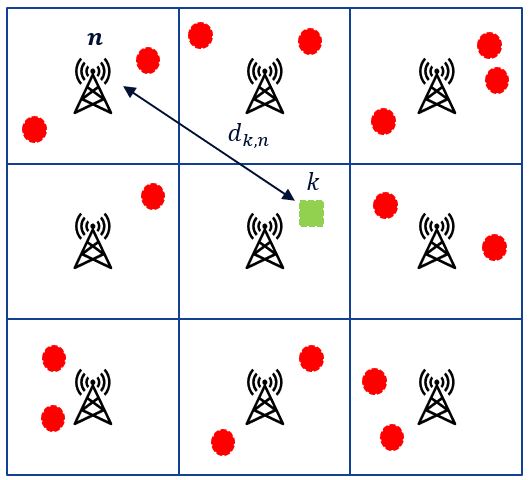
Figure 1: Example of the considered two-dimensional scenario with $N=9$ BSs.

II-A Channel Model

Assuming that antennas at the BSs are organized in a uniform linear array (ULA), the gain of the transmission toward AOD $\theta_{k}$ is given by vector $\bm{a}^{n}$, whose $m$ th component is [13]

$$[\bm{a}^{n}(\theta_{k})]_{m}=e^{j\delta_{k}}\exp\left(\frac{j2\pi\lambda(m-1)\cos(\theta_{k})}{d}\right),$$ (3)

where $[\bm{a}^{n}]_{m}$ denotes the $m-$ th element of vector $\bm{a}^{n}$, $m=1,\cdots,N_{a}$, $\lambda$ denotes the carrier wavelength, $d$ is the inter antenna spacing, $\delta_{k}$ is a user specific phase shift, and $j=\sqrt{-1}$.

The line of sight (LOS) component of the channel between the $n-$ th BS and UE $k$ is given by

$$\bm{h}_{\rm LOS}(k,n)=\sqrt{\frac{K_{0}}{d_{k,n}^{\nu}}}\bm{a}^{n}(\theta_{k}),$$ (4)

where $\nu$ is the path loss exponent and $K_{0}$ is a constant factor accounting for the cell edge signal to noise ratio (SNR).

We assume the Rice model for the small scale fading, and the channel can be modeled as the sum of a LOS path and a random multi-path component, i.e., [14, Ch. 2.4.2]

$$\bm{h}(k,n)=\sqrt{\frac{\Psi}{\Psi+1}}\bm{h}_{\rm LOS}(k,n)+\sqrt{\frac{1}{\Psi+1}}\bm{h}_{\rm NLOS}(k,n),$$ (5)

where $\Psi$ denotes the Rice factor and $\bm{h}_{\rm NLOS}(k,n)\sim\mathcal{CN}\left(\bm{0},K_{0}/d_{k,n}^{\nu}\bm{I}\right)$, with $\bm{0}$ and $\bm{I}$ being a vector with $N_{a}$ zero entries and the $N_{a}\times N_{a}$ identity matrix, respectively.

We assume that each BS serves a single UE per time instant by using a maximum ratio transmission (MRT) beamformer, and we denote as $\bm{g}(k,n)$ the MRT beamformer from BS $n$ toward UE $k$, given by

$$\bm{g}(k,n)=\frac{\bm{h}^{H}(k,n)}{||\bm{h}(k,n)||},$$ (6)

where $[\cdot]^{H}$ denotes the Hermitian of a vector.

BS $n$ transmits a symbol $q_{k}$ such that $\mathbb{E}[|q_{k}^{2}|]=1$ to UE $k$, and the received signal is expressed as

$$y_{k,n}=\bm{h}(k,n)\bm{g}(k,n)q_{k}\sqrt{P}+w,$$ (7)

where $P$ is the transmitted power and $w$ is the additive white Gaussian noise (AWGN) component distributed as a Gaussian r.v. with zero mean and variance $\sigma^{2}$.

The signal received by user $k$ suffers the interference caused by all BSs $\ell\neq n$ transmitting toward their scheduled UEs. The received SINR by UE $k$ is given by

$$\rho_{k,n}=\frac{|\bm{h}(k,n)\bm{g}(k,n)|^{2}P}{\sum_{\ell=1,\ell\neq n}^{N}|\bm{h}(k,\ell)\bm{g}(x_{\ell},\ell)|^{2}P+\sigma^{2}},$$ (8)

where $x_{\ell}$ denotes the index of the UE served by the $\ell$-th BS.

In this work, we consider two different UE scheduling policies, i.e., either round robin (RR) or proportional fair scheduling (PFS). When considering the semi-deterministic periodic traffic, we can assume a RR scheduling of the UEs at each BS, with a) the order properly selected in order to allow each UE to meet its latency requirement, and b) a fully loaded BS in terms of served UEs, i.e., in each TTI there is always a certain UE that needs to be scheduled by each BS. Therefore, with this RR scheduling, UEs in $\mathcal{X}_{n}$ are served in a deterministic fashion and, without loss of generality, we assume that they are sequentially served according to their index in $\mathcal{X}_{n}$. Note that, with these modeling assumptions, packets that are successfully received at the UEs always meet the latency constraints: on the other hand, when a packet transmission fails because of a wrong SINR prediction, the packet is just dropped, and that negatively affects the system reliability.

On the other hand, PFS [15] does not necessarily serve UEs in a deterministic fashion, and thus does not represent the most suitable solution for URLLC with extreme latency constraint. However, by guaranteeing the same long term average throughput, it has been widely used for MBB and its variations are envisioned to be used also for URLLC with not too extreme latency requirements [16]. Note that, to ensure UE fairness, PFS serves UEs in a certain TTI that have not been served in a while and therefore introduces some time periodicity in the interference power experienced by the UEs, in particular when the number of UEs per cell is not too high.

II-B Link Adaptation

LA is a technique used to control UEs quality of service in which, according to the channel condition, the BS chooses the best MCS in order to match a target BLER. Denoting as $\Omega$ the set of available MCS indexes, the LA problem for UE $k$ served by BS $n$ can be formulated as

$$\omega_{k}^{*}=\underset{\omega\in\Omega}{\arg\max}\,R_{k}(\omega|\hat{\rho_{k,n}})$$ (9a)

$$\text{s.t.}\quad\Gamma(\omega|\hat{\rho_{k,n}})\leq\Gamma_{0},$$ (9b)

where $\Gamma(\omega|\hat{\rho_{k,n}})$ and $R_{k}(\omega|\hat{\rho_{k,n}})$ are respectively the BLER and supported data rate given the estimated SINR $\hat{\rho_{k,n}}$ for user $k$ obtained choosing MCS $\omega$, and $\Gamma_{0}$ is the target BLER.

The basic LA algorithm is the OLLA where the estimated SINR value is modified based on the reception of the previously sent packets [6]. Therefore, in order to guarantee high reliability with very low latency with OLLA, for a long period of time the estimated SINR used for LA will be much lower than the actual one, i.e., $\hat{\rho_{k,n}}<<\rho_{k,n}$. The result is that reliability is obtained at the cost of wasting resources in terms of throughput. The OLLA algorithm is effective only when the target of the communication is not ultra reliability (for which the target BLER is set to $\Gamma_{0}=10^{-5}$, or even lower), or when one or few re-transmissions are allowed.

We hence note that, in order to guarantee a certain BLER while at the same time exploiting all the resources in terms of throughput, we need a good estimate of the SINR.

In this paper, we propose a novel approach to deal with the choice of the MCS based on the statistics of the SINR and in particular on the statistics of the interference power values (IPVs), exploiting the time correlation between successive IPVs. We target the maximization of the SE while ensuring a certain target BLER. A mathematical formulation of the problem will be given in the following sections.

III Interference Power Estimation

In order to choose the most suitable MCS, we need to be able to predict the behavior of the channel. In particular, considering that the received power from the serving cell varies in a much lower time scale when compared to the interference [17], we are interested in the estimation of the interference power. Considering a transmission from BS $n$ to UE $k$, the IPV random variable $I_{k}$ is given by the first term at the denominator in (8), i.e.,

$$I_{k}=\sum_{\ell=1,\ell\neq n}^{N}|\bm{h}(k,\ell)\bm{g}(x_{\ell},\ell)|^{2}P.$$ (10)

Since the IPV depends on the channel, which is a time dependent random process, for each given time instance $t$ the IPV can be represented as a random variable, i.e., $I_{k}(t)$. For a certain UE $k$, we consider $L$ IPVs in successive time instants, and we define the set $\mathcal{P}_{k}=\{I_{k}(1),\cdots,I_{k}(L)\}$ as the set of IPVs for UE $k$ during a time period $L$. The set $\mathcal{P}_{k}$ can be seen as an ergodic time series from which we can compute useful statistics for LA purposes. In the following, for the sake of clarity, we skip the subscript $k$ from the IPV random variable $I(t)$.

In particular, we are interested in the distribution of the IPV at time instant $t+1$ given $D$ previous IPVs observations, i.e., in the conditional probability $\mathbb{P}\left(I(t+1)|\bm{I}_{D}(t)\right)$, where $\bm{I}_{D}(t)=[I(t),\cdots,I(t-D+1)]$. This probability can be computed as

$$\mathbb{P}\left(I(t+1)|\bm{I}_{D}(t)\right)=\frac{\mathbb{P}\left(I(t+1),\bm{I}_{D}(t)\right)}{\mathbb{P}\left(\bm{I}_{D}(t)\right)}.$$ (11)

The marginal and joint distributions in (11) can respectively be computed from set $\mathcal{P}_{k}$ by shifting a length $D$ and $D+1$ window over the length $L$ series, where in the latter the sample at $D+1$ is the value to be predicted, i.e., that at $t+1$.

The simplest approach to estimate the probability density functions (PDFs) for each UE $k$ is to compute the empirical CDF $F_{k}(\bm{i})$ of $\mathcal{P}_{k}$ as

$$F_{k}(\bm{i})=\frac{\sum_{t=D}^{L}\mathds{1}(\bm{I}_{D}(t)<\bm{i})}{L-D+1},$$ (12)

where $\mathds{1}(\bm{I}_{D}(t)<\bm{i})$ is the counter of the number of vectors in $\mathcal{P}_{k}$ smaller than $\bm{i}$, where the inequality is component-wise. The empirical PDF is then derived from the CDF. However this method has the drawback that, if $L$ is not large enough, the entries with lower probability value will not appear in $\mathcal{P}_{k}$, and therefore we assume value $0$ for such entries. This problem becomes more prominent in the case of URLLC, since the extreme conditions that provide reliability with error probability of the very small magnitudes, e.g. $10^{-5}$, will be of focus. Using the histogram for such an application only makes sense if $L$ is large enough such that there are entries in the low probability part. In the next section we review the kernel based distribution estimation approach, which fills the gaps of the previously described distribution estimators.

IV Kernel Based PDF Estimation

We adopt the approach proposed in [18] to compute the joint PDF of the distribution of sets of $D$ and $D+1$ IPVs measured over consecutive time instants. These samples are filtered with the kernel function $\mathcal{K}$, from which we obtain the PDF [18]

$$f_{k}(\bm{i})=\frac{1}{L}\sum_{t=D}^{L}\mathcal{K}\left(\bm{i},\bm{I}_{D}(t),\gamma\right),$$ (13)

where $\bm{I}_{D}(t)$ is the $t$-th $D\times 1$ size vector of successive IPVs, $\bm{i}$ is the $D\times 1$ vector for which we want to compute the PDF, and $\gamma$ is an optimization parameter defined as the bandwidth. In order to compute the optimal bandwidth we exploit the key observation of [18] that the Gaussian kernel

$$\mathcal{K}\left(\bm{i},\bm{I}_{D}(t),\gamma\right)=\frac{1}{\sqrt{2\pi\gamma}}exp\left(-\frac{(\bm{i}-\bm{I}_{D}(t))^{H}(\bm{i}-\bm{I}_{D}(t))}{2\gamma}\right)$$ (14)

is the solution of the diffusion partial differential equation from which the optimal bandwidth is computed. Please refer to [18] for further details.

Once both $f_{k}\left(I(t+1),\bm{I}_{D}(t)\right)$ and $f_{k}\left(\bm{I}_{D}(t)\right)$ have been computed, we use (11) to obtain the conditional PDF

$$f_{k}\left(I(t+1)|\bm{I}_{D}(t)\right)=\frac{f_{k}\left(I(t+1),\bm{I}_{D}(t)\right)}{f_{k}\left(\bm{I}_{D}(t)\right)}.$$ (15)

In the next section, we propose different approaches which can be used for interference prediction.

V Interference prediction for link adaptation

Given the LA optimization problem (9), as in Section II-B, the choice of the MCS is based on the estimated SINR, and in particular on the predicted IPV. Based on this consideration, we rewrite the LA problem as

$$\min_{\hat{I}(t+1)} \quad\hat{I}(t+1)$$

s.t. $$\quad\mathbb{P}\left(\hat{I}(t+1)<I(t+1)|\bm{I}_{D}(t)\right)\leq\Gamma_{0},$$ (16)

where $\hat{I}(t+1)$ is the predicted IPV. The motivation of (16) is given in the following. Since we require to estimate the IPV for each time instant, in order to maximize the rate we choose the highest possible MCS. Thus we are interested in minimizing the value of the estimated IPV, while fulfilling the reliability requirement. According to the estimated SINR value, the BS chooses an MCS, which is assumed to cause an error if the estimated SINR is higher than the actual one. Therefore, as per our assumed model, the only source of uncertainty is the estimated IPV, i.e., an error occurs if the estimated IPV is below the actual one both computed at the successive time instant.

Remark: As opposed to the prediction methods in the literature in Section I, the proposed method does not rely on the channel model and can be used in all those scenarios for which traffic and therefore interference is assumed to have some time correlation.

V-A Expectation Based Prediction

In the EB prediction framework the choice of the interference power value to be used for LA is made by choosing the expected value given the previous $D$ observations of the interference power, i.e.,

$$I^{\rm(EM)}(t+1)=\mathrm{E}\left[I(t+1)|\bm{I}_{D}(t)\right],$$ (17)

where the expectation is computed empirically. Although simple, this approach has the drawback that it does not allow to control the BLER and in particular to upper bound it. Therefore, by exploiting the statistical knowledge of the conditional distribution of the successive IPVs, we propose the more conservative MQ framework.

V-B Maximum Quantile Prediction

A more conservative way of predicting the successive IPV and at the same time control the probability of error is obtained by considering a certain quantile of the CDF obtained by the conditional probability of the successive IPVs. In particular, we consider the fact that a transmission error occurs when the estimated SINR is above the actual one, and therefore, as we focus on IPV estimation, an error occurs when the estimated IPV is below the actual one.

On one hand, we aim at both minimizing the selected IPV in order to maximize the throughput and fulfilling the reliability constraint without choosing an unnecessarily low IPV. On the other hand, the CDF function in the (16) is a monotonically decreasing function of $\hat{I}(t+1)$ by definition, thus the optimal solution shall fulfill (16) with equality:

$$I^{\rm(MQ)}(t+1)=\hat{I}(t+1)$$ (18a)

$$\text{s.t.}\quad\mathbb{P}\left(\hat{I}(t+1)<I(t+1)|\bm{I}_{D}(t)\right)=\Gamma_{0}.$$ (18b)

VI Numerical Results

We here compare the results achieved with the proposed EB and MQ heuristics against some state of the art techniques. We consider a scenario with $N=9$ cells, where the distance between neighboring BSs is $200$ m, and each BS is equipped with $N_{a}=16$ antennas linearly spaced by $d=\lambda/2$. The IPVs are measured in the central cell, and the number of UEs in the surrounding cells is distributed between $K_{\rm min}=2$ and $K_{\rm max}=8$. We consider a noise power of $\sigma^{2}=-101$ dBm, a transmitted power at each BS of $P=46$ dBm, $\Psi=10$ dB, $\nu=3.5$ and $K_{0}$ ensures a cell edge SNR of $20$ dB. Results are obtained by considering that the scheduling process over the entire network generates a total number $T=3\cdot 10^{6}$ IPVs. We consider $D=1$ for both the proposed EB and MQ, i.e., based on the IPV estimated at the current time instant, the methods chose an IPV at the successive time instant. We assume as a correct transmission the event in which the predicted IPV is greater than the actual one at the successive time instant, whereas otherwise we consider a failure: this models a system where re-transmissions are not allowed. For each sequence of length $T$, we test the reliability of the different solutions by counting the number of events in which the predicted IPV is below the actual one, and we consider this value as a proxy of the system reliability. We hence define the reliability of the system as

$$\theta=\frac{\sum_{t=1}^{T-1}\chi(t)}{T-1},$$ (19)

where $\chi(t)$ is the indicator function of the predicted IPV being lower than the actual one, i.e.,

$$\chi(t)=\begin{cases}1\quad\text{if}\,\hat{I}(t+1)<I(t+1);\\ 0\quad\text{otherwise}.\end{cases}$$ (20)

For each UE we assume that, if a failure happens, the experienced SE is zero. Therefore the instantaneous UE SE $R(t)$ at time $t$ is computed as

$$R(t)=(1-\chi(t))\log_{2}(1+\hat{\rho}(t)),$$ (21)

with $\hat{\rho}(t)$ being the predicted SINR.

Results are compared against a method based on [7, Eq. (8)], where the prediction is obtained by low pass filtering the previous estimated IPV with the current one, i.e.,

$$\hat{I}(t+1)=\alpha I(t)+(1-\alpha)\hat{I}(t-1).$$ (22)

We denote this method as LPP (low-pass prediction). However, note that (22) has been shown as effective only for URLLC when OLLA with one re-transmission is available.

Furthermore, we compare our method against the idea proposed in [19], where authors perform IPV prediction based on the marginal PDF of the interference. We extend then the proposed approach by applying both the EB and MQ prediction methods to the marginal PDF $f_{k}\left(I(t)\right)$.

Fig. 2 shows the average SE $R$ versus the average $\theta$ for RR scheduling with $L=\{50,100,500,5000,10000\}$ and $\Gamma_{0}=10^{-3}$. We first observe that both the MQ methods on the marginal and conditional PDF obtain much better average SE and $\theta$ when compared to other schemes, as MQ has been properly designed to control the probability of error without re-transmissions. Furthermore we note that, as $L$ increases, the average $\theta$ decreases for both the MQ methods on the conditional and on marginal PDFs. Finally, for each value of $L$ we highlight that the MQ on conditional PDF achieves about $10\%$ higher average rate for the same average $\theta$ when compared to the MQ on the marginal PDF, showing the merits of our proposed approach that exploits time correlation of the interference. Finally, we highlight that both the EB methods and LPP do not lead to any better performance when increasing $L$: this is due to the fact that, differently from the MQ methods, none of these prediction methods has control on the target reliability.

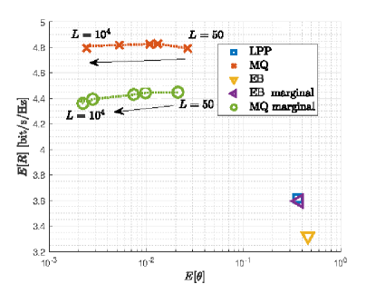
Figure 2: Average SE $R$ versus average $\theta$ for RR with $L=\{50,100,500,5000,10000\}$ and $\Gamma_{0}=10^{-3}$.

Fig. 3 shows the CDF $F(\theta)$ of $\theta$ for RR scheduling with $\Gamma_{0}=10^{-3}$ and $L=5000$. The CDFs of the MQ methods are almost the same, and they present a significant performance gain when compared to the other methods. Furthermore, we observe that the MQ methods try to meet the target BLER requirement fixed to $\Gamma_{0}=10^{-3}$ as both CDFs are centered around that value.

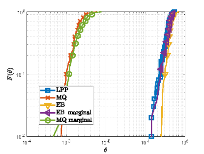
Figure 3: CDF $F(\theta)$ of $\theta$ for RR with $L=5000$ and $\Gamma_{0}=10^{-3}$.

Fig. 4 shows the average SE $R$ versus the average $\theta$ for RR scheduling with $L=5000$ and $\Gamma_{0}=\{10^{-1},5\cdot 10^{-2},10^{-2},5\cdot 10^{-3},10^{-3},5\cdot 10^{-4},10^{-4},10^{-5}\}$. Similar as before, the proposed MQ method strongly outperforms LPP and both the EB methods in terms of both average SE and $\theta$. Then, also in this setup with different values of $\Gamma_{0}$, the MQ method based on the conditional PDF achieves almost the same reliability value $\theta$ of the MQ based on the marginal PDF but providing higher SE. This further justifies our proposal of using the conditional PDF. Finally, as $\Gamma_{0}$ increases, we notice that the average rate initially increases, while it decreases after a certain point. This is due to the fact that with higher reliability, i.e., lower values of $\Gamma_{0}$, we tend to be more conservative and waste part of the rate resources that could be used, whereas with lower reliability target, i.e., higher values of $\Gamma_{0}$, the pre-log factor in (21) becomes dominant and therefore the average rate is lowered by the lower success probability.

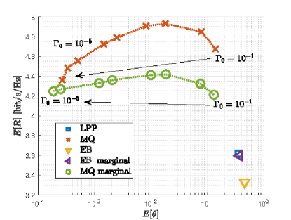
Figure 4: Average SE $R$ versus average $\theta$ for RR with $L=5000$ and $\Gamma_{0}=\{10^{-1},5\cdot 10^{-2},10^{-2},5\cdot 10^{-3},10^{-3},5\cdot 10^{-4},10^{-4},10^{-5}\}$.

Although in the considered scenario we have a different number of UEs per cell, with RR there is more time correlation of the interference as the scheduling in each cell is deterministic. Therefore, Fig. 5 shows the average SE $R$ versus the average $\theta$ for PFS with $L=5000$ and $\Gamma_{0}=\{10^{-1},5\cdot 10^{-2},10^{-2},5\cdot 10^{-3},10^{-3},5\cdot 10^{-4},10^{-4},10^{-5}\}$. The increasing and decreasing behavior of the average SE for increasing values of $\Gamma_{0}$ is justified by the same considerations done for the RR case. Results show that also in the PFS case the MQ solutions perform better than LPP and EB methods. Furthermore, we highlight that also in this case MQ based on the conditional PDF is advantageous in terms of average SE when compared to MQ based on the marginal PDF, although the performance gain is much less than that obtained with RR. This shows that, also with PFS, there is a certain periodicity in the scheduling, which can still be exploited in order to improve system performance.

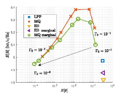
Figure 5: Average SE $R$ versus average $\theta$ for PFS with $L=5000$ and $\Gamma_{0}=\{10^{-1},5\cdot 10^{-2},10^{-2},5\cdot 10^{-3},10^{-3},5\cdot 10^{-4},10^{-4},10^{-5}\}$.

VII Conclusions

In this paper, we considered the problem of interference prediction for URLLC traffic. The main motivation behind this work is that, in order to guarantee both the required reliability and at the same time not wasting resources when performing LA, we must be able to accurately predict the SINR in order to choose a proper MCS. Considering then that URLLC with most extreme latency and reliability requirements is characterized by semi-deterministic periodic traffic, we treated interference as a time series. By exploiting the inherent time correlation, we designed two prediction algorithms based on the conditional PDF, namely EB and MQ. We compared the proposed solutions against state of the art algorithms, and showed that the MQ based on the conditional PDF is a promising solution for URLLC, as it allows to control reliability while at the same time optimizing the resources in terms of SE.

VIII Acknowledgments

The authors would like to thank their colleagues S. Mandelli, S. Klein, and A. Weber for the numerous helpful discussions.

References

- [1] 3GPP, “Service requirements for cyber-physical control applications in vertical domains,” 3rd Generation Partnership Project (3GPP), TS 22.104, 2019.
- [2] G. Durisi, T. Koch, and P. Popovski, “Toward massive, ultrareliable, and low-latency wireless communication with short packets,” Proc. of the IEEE, vol. 104, no. 9, pp. 1711–1726, 2016.
- [3] C.-P. Li, J. Jiang, W. Chen, T. Ji, and J. Smee, “5G ultra-reliable and low-latency systems design,” in 2017 European Conf. on Networks and Commun. (EuCNC). IEEE, 2017, pp. 1–5.
- [4] M. Bennis, M. Debbah, and H. V. Poor, “Ultrareliable and low-latency wireless communication: Tail, risk, and scale,” Proc. of the IEEE, vol. 106, no. 10, pp. 1834–1853, 2018.
- [5] H. Shariatmadari, Z. Li, M. A. Uusitalo, S. Iraji, and R. Jäntti, “Link adaptation design for ultra-reliable communications,” in 2016 IEEE International Conf. on Commun. (ICC). IEEE, 2016, pp. 1–5.
- [6] A. Sampath, P. S. Kumar, and J. M. Holtzman, “On setting reverse link target SIR in a CDMA system,” in 1997 IEEE 47th Vehicular Tech. Conf. Technology in Motion, vol. 2. IEEE, 1997, pp. 929–933.
- [7] G. Pocovi, K. I. Pedersen, and P. Mogensen, “Joint link adaptation and scheduling for 5G ultra-reliable low-latency communications,” IEEE Access, vol. 6, pp. 28 912–28 922, 2018.
- [8] U. Oruthota, F. Ahmed, and O. Tirkkonen, “Ultra-reliable link adaptation for downlink MISO transmission in 5G cellular networks,” Information, vol. 7, no. 1, p. 14, 2016.
- [9] T. Levanen, J. Venalainen, and M. Valkama, “Interference analysis and performance evaluation of 5G flexible-TDD based dense small-cell system,” in 2015 IEEE 82nd Vehicular Tech. Conf. (VTC2015-Fall). IEEE, 2015, pp. 1–7.
- [10] M. Taranetz and M. Rupp, “A circular interference model for heterogeneous cellular networks,” IEEE Trans. on Wireless Commun., vol. 15, no. 2, pp. 1432–1444, 2015.
- [11] K. Feng and M. Haenggi, “On the location-dependent SIR gain in cellular networks,” IEEE Wireless Commun. Letters, vol. 8, no. 3, pp. 777–780, 2019.
- [12] Y. Zhuang, Y. Luo, L. Cai, and J. Pan, “A geometric probability model for capacity analysis and interference estimation in wireless mobile cellular systems,” in 2011 IEEE Global Telecom. Conf. (GLOBECOM). IEEE, 2011, pp. 1–6.
- [13] C. A. Balanis, Antenna theory: analysis and design. John wiley & sons, 2016.
- [14] D. Tse and P. Viswanath, Fundamentals of wireless communication. Cambridge university press, 2005.
- [15] P. Viswanath, D. N. C. Tse, and R. Laroia, “Opportunistic beamforming using dumb antennas,” IEEE Trans. on Inform. Theory, vol. 48, no. 6, pp. 1277–1294, 2002.
- [16] E. Sisinni and F. Tramarin, “Isochronous wireless communication system for industrial automation,” in Industrial Wireless Sensor Networks. Elsevier, 2016, pp. 167–188.
- [17] H. Holma and A. Toskala, LTE advanced: 3GPP solution for IMT-Advanced. John Wiley & Sons, 2012.
- [18] Z. I. Botev, J. F. Grotowski, D. P. Kroese et al., “Kernel density estimation via diffusion,” The annals of Statistics, vol. 38, no. 5, pp. 2916–2957, 2010.
- [19] S. Klein and S. Mandelli, “Link adaptation in telecommunication systems,” 2019, filed patent application.