A pressure robust staggered discontinuous Galerkin method
for the Stokes equations

Abstract: In this paper we propose a pressure robust staggered discontinuous Galerkin method for the Stokes equations on general polygonal meshes by using piecewise constant approximations. We modify the right hand side of the body force in the discrete formulation by exploiting divergence preserving velocity reconstruction operator, which is the crux for pressure independent velocity error estimates. The optimal convergence for velocity gradient, velocity and pressure are proved. In addition, we are able to prove the superconvergence of velocity approximation by the incorporation of divergence preserving velocity reconstruction operator in the dual problem, which is also an important contribution of this paper. Finally, several numerical experiments are carried out to confirm the theoretical findings.

Keywords: staggered DG method, the Stokes equations, superconvergence, polygonal mesh, divergence preserving velocity reconstruction, pressure-robustness

1 Introduction

In this paper we consider the following Stokes equations: Find the velocity $\bm{u}:\Omega\rightarrow\mathbb{R}^{2}$ and the pressure $p:\Omega\rightarrow\mathbb{R}$ such that

$$\begin{split}-\nu\Delta\bm{u}+\nabla p&=\bm{f}\hskip 8.5359pt\mbox{in}\;\Omega,\\ \nabla\cdot\bm{u}&=0\quad\mbox{in}\;\Omega,\\ \bm{u}&=0\quad\mbox{on}\;\partial\Omega,\end{split}$$ (1.1)

where $\Omega$ is the computational domain in $\mathbb{R}^{2}$, $\nu>0$ is a constant viscosity parameter and $\bm{f}\in[L^{2}(\Omega)]^{2}$ is the body force.

A large amount of work has been dedicated to solving (1.1), see [25, 32] and the references therein. However, classical finite element methods can not deliver exactly divergence free solutions in the sense of $H(\text{div};\Omega)$ and the divergence constraint is relaxed in order to guarantee inf-sup stability [29]. As such, these methods suffer from a lack of pressure robustness, specifically, their velocity error estimates are pressure dependent and possibly deteriorates unboundedly for $\nu\rightarrow 0$, which shows some kind of locking phenomena in the sense of [2].

To remedy this issue, various approaches have been proposed. Exactly divergence-free $H^{1}(\Omega)$ or $H(\text{div};\Omega)$ conforming methods of order $k$ is developed in [43, 50, 22]. An alternative strategy to achieve divergence-free property is to enrich the $H(\text{div};\Omega)$-conforming elements with divergence free rational functions, which provides the correct flexibility to enforce (strong) continuity (cf. [26, 27]). Moreover, Cockburn [17] and Wang [46] modify the variational formulation and introduce the tangential penalty and thus obtain discontinuous Galerkin divergence-free schemes. Another approach that can deliver pressure independent error estimates is to add grad-div stabilization [41, 40]. Recently, a method based on modifying the right hand side is shown to be able to retrieve pressure robustness, and this strategy has been successfully applied to finite volume method [34], the nonconforming Crouzeix-Raviart element [35, 5], the conforming $P_{2}^{+}-P_{1}^{\text{disc}}$ element [36], the hybrid discontinuous Galerkin method [20], low and high order Taylor-Hood and mini elements [33], hybrid high-order (HHO) method [42] and weak Galerkin (WG) method [39].

Recently, polygonal finite element methods have become a hot topic due to their great flexibility in handling complicated geometries. Various approaches in the framework of polygonal grids have been proposed to solve partial differential equations arising from practical applications, such as virtual element method (VEM) [3, 4], mimetic finite difference methods [38], HHO method [19, 18], WG methods [47, 48], generalized barycentric coordinates methods [44], staggered discontinuous Galerkin (SDG) method [52, 56], etc. SDG as the new generation discretisation methods for PDEs based on discrete unknowns that enjoys staggered continuity properties is initially introduced to solve wave propagation problem [12, 13]. Its close connection to a hybridizable DG method is unveiled in [10, 11]. Note that SDG method differs from other DG methods in the sense that the basis functions are locally conforming and penalty terms are not required. This method has many desirable features and has been successfully applied to a wide range of partial differential equations [9, 21, 52, 56, 53, 54, 51, 55, 31].

The purpose of this paper is to develop a pressure robust staggered discontinuous Galerkin (PR-SDG) method on general polygonal meshes for the Stokes equations with piecewise constant approximations. Our approach is based on the framework of lowest order SDG method introduced in [56]. The novelty here is to exploit velocity reconstruction operator in the discretization of the source term in the spirit of [34, 39]. The principal idea behind this is that discrete divergence-free velocity test functions are mapped to exact divergence-free ones by velocity reconstruction operator. The crux of SDG method for the Stokes equations is to generate a sub-triangulation by connecting an interior point of the polygonal grid to all the vertices of the polygon. Then finite element spaces that enjoy staggered continuity properties for velocity gradient, velocity and pressure are developed, which naturally lead to inf-sup stable pairs. In particular, the velocity space is continuous over the edges of the polygon, which enables us to establish velocity reconstruction operator based on the polygonal grid. A rigorous convergence analysis for $L^{2}$ errors of velocity gradient, velocity and pressure is investigated. The main difficulty lies in the proof of superconvergence and traditional techniques no long work. To attack this issue, we exploit Aubin-Nitsche duality argument with nonstandard incorporation of continuous and discrete formulation of the dual problem; in addition, velocity reconstruction operator is employed in the discretization of the dual problem. We keep track explicitly of the dependence on the viscosity in the analysis so as to address the practically important issue of body forces with large irrotational part. Note that the lowest order SDG method can be viewed as finite volume method, thus our work provides new perspectives for the understanding of finite volume method. Indeed, our primal and dual partitions are exactly the same as the finite volume method proposed in [49], whereas our method is based on the first order system and piecewise constant functions are exploited for all the involved unknowns. Importantly, the continuity of all the unknowns are staggered on the interelement boundaries, which naturally yields a stable numerical scheme without resorting to further stabilization. We emphasize that the development of pressure robust method with velocity reconstruction operator on polygonal mesh is still in its infancy [8, 39], the approach developed in this paper will definitely inspire more works in this direction.

The rest of the paper is organized as follows. In the next section, we formulate the PR-SDG method for the Stokes equations based on velocity reconstruction operator. Then in section 3, we prove the optimal convergence for $L^{2}$ errors of velocity gradient, velocity and pressure as well as superconvergence of velocity. Several numerical experiments are carried out in section 4 to verify the proposed theories. Finally, a conclusion is given.

2 Description of PR-SDG method

In this section we begin with introducing the construction of minimal degree $H(\text{div};\Omega)$ conforming function on convex polygon. Then we propose the PR-SDG method by employing $H(\text{div};\Omega)$ conforming velocity reconstruction in the discretization of the body force. Finally, some fundamental properties inherited from the proposed method are provided.

2.1 Preliminaries

Letting $L^{2}_{0}(\Omega):=\{q\in L^{2}(\Omega):\int_{\Omega}q\;dx=0\}$, the weak formulation for (1.1) reads as follows: Find $(\bm{u},p)\in[H^{1}_{0}(\Omega)]^{2}\times L^{2}_{0}(\Omega)$ such that

$$\begin{split}a(\bm{u},\bm{v})+b(\bm{v},p)&=(\bm{f},\bm{v})\quad\forall\bm{v}\in[H^{1}_{0}(\Omega)]^{2},\\ b(\bm{u},q)&=0\hskip 31.2982pt\forall q\in L^{2}_{0}(\Omega),\end{split}$$ (2.1)

where

$$a(\bm{u},\bm{v})=(\nu\nabla\bm{u},\nabla\bm{v}),\quad b(\bm{v},q) =-(q,\nabla\cdot\bm{v}).$$

The weak formulation (2.1) is well posed thanks to the coercivity of the bilinear form $a$ and the inf–sup stability of the bilinear $b$, see [25].

We introduce an auxiliary unknown $\bm{\omega}=\nu\nabla\bm{u}$. Then, the model problem (1.1) can be recast into the following first order system of equations

$$\bm{\omega}-\nu\nabla\bm{u} =\bm{0}\hskip 11.38092pt\mbox{in}\;\Omega,$$ (2.2a)

$$-\nabla\cdot\bm{\omega}+\nabla p =\bm{f}\quad\mbox{in}\;\Omega,$$ (2.2b)

$$\nabla\cdot\bm{u} =0\hskip 11.38092pt\mbox{in}\;\Omega,$$ (2.2c)

$$\bm{u} =\bm{0}\hskip 11.38092pt\mbox{on}\;\partial\Omega.$$ (2.2d)

Before closing this subsection we introduce some notations that will be employed throughout the paper. Let $D\subset\mathbb{R}^{d},$ $d=1,2$, we adopt the standard notations for the Sobolev spaces $H^{s}(D)$ and their associated norms $\|\cdot\|_{s,D}$, and semi-norms $|\cdot|_{s,D}$ for $s\geq 0$. The space $H^{0}(D)$ coincides with $L^{2}(D)$, for which the norm is denoted as $\|\cdot\|_{D}$. We use $(\cdot,\cdot)_{D}$ to denote the inner product for $d=1,2$. If $D=\Omega$, the subscript $\Omega$ will be dropped unless otherwise mentioned. In the sequel, we use $C$ to denote a generic positive constant which may have different values at different occurrences.

2.2 $H(\text{div})$ conforming function on polygon

In this subsection, we briefly introduce the construction of $H(\text{div};\Omega)$ conforming function on convex polygon by following [7]. Let $T$ be a polygon with $m$ vertices $\mathsf{v}_{i}$ that are arranged counterclockwise, and let $\bm{n}_{i}(1\leq i\leq m)$ be the outward unit normal vector on edge $e_{i}$ that connects vertices $\mathsf{v}_{i}$ and $\mathsf{v}_{i+1}$, where we conveniently denote $\mathsf{v}_{j}=\mathsf{v}_{j(mod\,m)}$ when the subscript $j$ is not in the range of $\{1,\cdots,m\}$, see Figure 1 for an illustration. Let $\mathsf{x}$ be an interior point of $T$, its distance to edge $e_{i}$ and a scaled normal vector are defined as

$$d_{i}=(\mathsf{v}_{i}-\mathsf{x})\cdot\bm{n}_{i},\quad\tilde{\bm{n}}_{i}=\frac{1}{d_{i}}\bm{n}_{i}\quad 1\leq i\leq m.$$

Then the Wachspress coordinates are defined as (cf. [45])

$$\lambda_{i}=w_{i}(x)/W(x)\quad 1\leq i\leq m,$$

where $w_{i}(x)=\text{det}(\tilde{\bm{n}}_{i},\tilde{\bm{n}}_{i+1})$, $W(x)=\sum_{i=1}^{m}w_{i}(x)$.

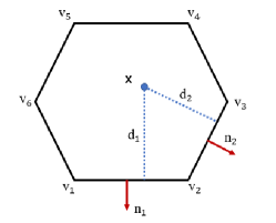
Figure 1: Schematic of Wachspress coordinates on a hexagon.

As discusses in [23], one introduces an auxiliary ratio function

$$R_{i}(x)=\frac{\nabla w_{i}(x)}{w_{i}(x)}\quad 1\leq i\leq m.$$

By the quotient rule for differentiation, one is led to

$$\nabla\lambda_{i}(x)=\lambda_{i}(x)(R_{i}-\sum_{j=1}^{m}\lambda_{j}R_{j})\quad 1\leq i\leq m.$$

Then, a counterclockwise $90^{o}$ rotation of the gradient is defined by

$$\text{curl}(\lambda_{i})=\left(\begin{array}[]{c}-\partial_{y}\lambda_{i}\\ \partial_{x}\lambda_{i}\\ \end{array}\right)=\left(\begin{array}[]{cc}0&-1\\ 1&0\\ \end{array}\right)\nabla\lambda_{i}(x)\quad 1\leq i\leq m.$$

Now we are ready to present the construction of minimal degree $H(\text{div};\Omega)$ conforming finite element function on convex polygon. Denote $|T|,|e_{i}|$ as the area and the length of edge $e_{i}$ for $1\leq i\leq m$. Let $\mathsf{x}_{*}$ be an arbitrary point inside polygon $T$, and denote by $|T_{i}|$ the area of the triangle formed by $\mathsf{x}_{*},\mathsf{v}_{i},\mathsf{v}_{i+1}$. Then for each $1\leq i\leq m$, we define $\bm{\varphi}_{i}$ by

$$\bm{\varphi}_{i}=c_{i,0}(\mathsf{x}-\mathsf{x}_{*})+\sum_{k=1}^{m}c_{i,k}\text{curl}\lambda_{k},$$

where $c_{i,0}=\frac{|e_{i}|}{2|T|}$, $c_{i,k}=-\frac{1}{m}\sum_{l=1}^{m-1}lb_{i,k+l}$ and $b_{i,l}=\delta_{i,l}|e_{l}|-|e_{i}|\frac{|T_{l}|}{|T|}$. Here $\delta_{i,l}$ is the Kronecker symbol.

Furthermore, for these basis functions, we have the following properties

$$\bm{\varphi}_{i}|e_{j}\cdot\bm{n}_{j}=\delta_{i,j}\quad\nabla\cdot\bm{\varphi}_{i}=2c_{i,0}\quad\forall 1\leq i,j\leq m.$$

Lemma 2.1.

For $1\leq i\leq m$, one has [7]

$$\|\bm{\varphi}_{i}\|_{0,T}\leq C(m)|e_{i}|.$$

In addition, for $\bm{\xi}\in[H^{1}(T)]^{2}$, we have

$$\|\bm{\xi}-\Pi^{RT}\bm{\xi}\|_{0,T}\leq C(m)h_{T}\|\bm{\xi}\|_{1,T}.$$

Let $\Pi^{0}$ be the nodal value interpolation operator based on the generalized barycentric coordinates such as Wachspress coordinates (cf. [45]). For any $\phi\in W^{1,p}(T),p>2$, it holds (cf. [7])

$$\Pi^{RT}\textnormal{curl}\,\phi=\textnormal{curl}\,\Pi^{0}\phi.$$ (2.3)

2.3 Construction of PR-SDG method

In this subsection we will present the construction of PR-SDG method. To begin with, we will describe the construction of the staggered mesh needed in our method by following [12, 13, 14, 30]. We let $\mathcal{T}_{u}$ be the initial partition of the domain $\Omega$ into non-overlapping simple convex polygonal elements (primal mesh). We use $\mathcal{F}_{u}$ to represent the set of all the edges in this partition (primal edges) and $\mathcal{F}_{u}^{0}$ to represent the subset of all interior edges, that is, $\mathcal{F}_{u}^{0}=\mathcal{F}_{u}\setminus\partial\Omega$. For each polygon $T$ in the initial partition $\mathcal{T}_{u}$, we select an interior point $\mathsf{x}_{*}$ and create new edges by connecting $\mathsf{x}_{*}$ to the vertices of polygon. This process will divide $T$ into the union of triangles, where the triangle is denoted as $\tau$. Moreover, we will use $\mathcal{F}_{p}$ to denote the set of all the new edges generated by this subdivision process (dual edges) and use $\mathcal{T}_{h}$ to denote the resulting triangulation (simplicial submeshes), on which our basis functions are defined. In addition, we define $\mathcal{F}:=\mathcal{F}_{u}\cup\mathcal{F}_{p}$ and $\mathcal{F}^{0}:=\mathcal{F}_{u}^{0}\cup\mathcal{F}_{p}$. This construction is illustrated in Figure 2, where solid lines are edges in $\mathcal{F}_{u}$ and dashed lines are edges in $\mathcal{F}_{p}$. For each triangle $\tau\in\mathcal{T}_{h}$, we let $h_{\tau}$ be the diameter of $\tau$ and $h=\max\{h_{\tau},\tau\in\mathcal{T}_{h}\}$. Here we assume that the primal partition satisfies the standard mesh regularity assumptions: 1) Every primal element $T$ is star-shaped with respect to a ball of radius $\rho_{B}h_{T}$, where $\rho_{B}$ is a positive constant. 2) For every primal element $T$ and every edge $e\in\partial T$, it satisfies $|e|\geq\rho_{E}h_{T}$, where $\rho_{E}$ is a positive constant. Note that these assumptions can guarantee that the resulting triangulation $\mathcal{T}_{h}$ is shape regular.

For each interior edge $e\in\mathcal{F}_{u}^{0}$, we use $D(e)$ to denote the dual mesh, which is the union of the two triangles in $\mathcal{T}_{h}$ sharing the edge $e$, and for each boundary edge $e\in\mathcal{F}_{u}\backslash\mathcal{F}_{u}^{0}$, we use $D(e)$ to denote the triangle in $\mathcal{T}_{h}$ having the edge $e$, see Figure 2. We define a unit normal vector $\bm{n}_{e}$ on each edge $e\in\mathcal{F}$ as follows: If $e\in\mathcal{F}\backslash\mathcal{F}^{0}$ is a boundary edge, then we define $\bm{n}_{e}$ as the unit normal vector of $e$ pointing towards outside of $\Omega$. If $e\in\mathcal{F}^{0}$ is an interior edge, then we fix $\bm{n}_{e}$ as one of the two possible unit normal vectors on $e$. We will use $\bm{n}$ instead of $\bm{n}_{e}$ to simplify the notation when there is no confusion.

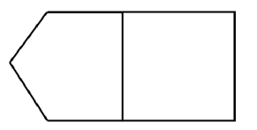
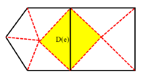
Figure 2: Illustration of primal mesh (left) and the resulting simplicial submeshes (right). Solid lines represent primal edges and dashed lines represent dual edges.

Let $k\geq 0$ be the order of approximation. For every $\tau\in\mathcal{T}_{h}$ and $e\in\mathcal{F}$, we define $P_{k}(\tau)$ and $P_{k}(e)$ as the spaces of polynomials of degree less than or equal to $k$ on $\tau$ and $e$, respectively. Now we are ready to describe the finite element spaces that will be used to define our numerical scheme. First, the locally $H^{1}(\Omega)$ conforming SDG space for velocity is defined as:

$$S_{h}:=\{\bm{v}:\bm{v}\mid_{D(e)}\in[P_{0}(D(e))]^{2},\forall e\in\mathcal{F}_{u};\bm{v}\mid_{D(e)}=0\;\mbox{if}\;e\in\mathcal{F}_{u}\backslash\mathcal{F}_{u}^{0}\}.$$

The degrees of freedom for this space can be described as (see Figure 3)

$$\phi_{e}(\bm{v}):=(\bm{v},\bm{\varsigma})_{e}\quad\forall\bm{\varsigma}\in[P_{0}(e)]^{2},e\in\mathcal{F}_{u}.$$

The discrete $L^{2}$ norm and $H^{1}$ norm for the space $S_{h}$ are given by

$$\begin{split}\|\bm{v}\|_{X}^{2}&=\|\bm{v}\|_{0}^{2}+\sum_{e\in\mathcal{F}_{u}^{0}}h_{e}\|\bm{v}\|_{0,e}^{2},\\ \|\bm{v}\|_{h}^{2}&=\sum_{e\in\mathcal{F}_{p}}h_{e}^{-1}\|[\bm{v}]\|_{0,e}^{2}.\end{split}$$

Here $\bm{v}_{i}=\bm{v}|_{\tau_{i}},i=1,2$ and $[\bm{v}]=\bm{v}_{1}-\bm{v}_{2}$ denotes the jump on an interior edge that is shared by two triangles $\tau_{1}$ and $\tau_{2}$ belonging to $\mathcal{T}_{h}$, and we simply take $[\bm{v}]=\bm{v}_{1}$ for $e\in\mathcal{F}_{u}\backslash\mathcal{F}_{u}^{0}$.

Next, the locally $H(\mbox{div};\Omega)$ conforming SDG space for the velocity gradient approximation is defined as:

$$V_{h}:=\{\bm{\psi}:\bm{\psi}\mid_{\tau}\in[P_{0}(\tau)]^{2\times 2},\forall\tau\in\mathcal{T}_{h};[\bm{\psi}\bm{n}]\mid_{e}=0,\forall e\in\mathcal{F}_{p}\},$$

which is equipped by

$$\|\bm{\psi}\|_{X^{\prime}}^{2}=\|\bm{\psi}\|_{0}^{2}+\sum_{e\in\mathcal{F}_{p}}h_{e}\|\bm{\psi}\bm{n}\|_{0,e}^{2}.$$

Invoking scaling arguments, we have

$$\|\bm{\psi}\|_{0}\leq\|\bm{\psi}\|_{X^{\prime}}\leq C\|\bm{\psi}\|_{0}.$$ (2.4)

We define the following degrees of freedom for $V_{h}$ and it is illustrated in Figure 3

$$\varphi_{e}(\bm{\psi}):=(\bm{\psi}\bm{n},\bm{\varsigma})_{e}\quad\forall\bm{\varsigma}\in[P_{0}(e)]^{2},e\in\mathcal{F}_{p}.$$

In the above definition, the jump $[\bm{\psi}\bm{n}]$ over an edge $e\in\mathcal{F}_{p}$ is defined as

$$[\bm{\psi}\bm{n}]=\bm{\psi}_{1}\bm{n}-\bm{\psi}_{2}\bm{n},$$

where $\bm{\psi}_{i}=\bm{\psi}|_{\tau_{i}}$, $e$ is the common edge of the two triangles $\tau_{1}$ and $\tau_{2}$ that belong to $\mathcal{T}_{h}$, and $\bm{n}$ is a unit normal to the edge $e$.

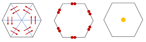
Figure 3: Schematic of degrees of freedom for $V_{h}$ (left), $S_{h}$ (middle) and $P_{h}$ (right) over the polygon.

Finally, locally $H^{1}(\Omega)$ conforming finite element space for pressure is defined as:

$$P_{h}:=\{q:q\mid_{T}\in P_{0}(T),\;\forall T\in\mathcal{T}_{u};\int_{\Omega}q\;dx=0\}$$

with norm

$$\|q\|_{P}^{2}=\|q\|_{0}^{2}+\sum_{e\in\mathcal{F}_{p}}h_{e}\|q\|_{0,e}^{2}.$$

Now let us define the $H(\text{div};\Omega)$ conforming interpolation operator on polygonal mesh in the spirit of [7]. For any $\bm{v}\in H(\text{div};\Omega)+S_{h}$, we define $\Pi^{RT}\bm{v}$ restricted to $T$ by

$$\Pi^{RT}\bm{v}=\sum_{i=1}^{m}r_{i}(\bm{v})\bm{\varphi}_{i},$$

where

$$r_{i}(\bm{v})=\frac{1}{|e_{i}|}\int_{e_{i}}\bm{v}\cdot\bm{n}\;ds\quad\forall e\in\mathcal{F}_{u}\cap\partial T,T\in\mathcal{T}_{u}.$$

Note that any function $\bm{v}\in S_{h}$ is continuous over the edge $e\in\mathcal{F}_{u}$, which by definition yields a function $\Pi^{RT}\bm{v}$ that belongs to $H(\text{div};\Omega)$.

Then following [56], the discrete formulation for the Stokes equations (2.2) reads as follows: Find $(\bm{\omega}_{h},\bm{u}_{h},p_{h})\in V_{h}\times S_{h}\times P_{h}$ such that

$$B_{h}(\bm{\omega}_{h},\bm{v})+b_{h}^{*}(p_{h},\bm{v}) =(\bm{f},\Pi^{RT}\bm{v})\hskip 28.45274pt\forall\bm{v}\in S_{h},$$ (2.5a)

$$B_{h}^{*}(\bm{u}_{h},\bm{\psi}) =\nu^{-1}(\bm{\omega}_{h},\bm{\psi})\hskip 27.03003pt\forall\bm{\psi}\in V_{h},$$ (2.5b)

$$b_{h}(\bm{u}_{h},q) =0\hskip 71.13188pt\forall q\in P_{h},$$ (2.5c)

where the bilinear forms $B_{h}(\bm{\omega}_{h},\bm{v})$ and $B_{h}^{*}(\bm{u}_{h},\bm{\psi})$ are defined as

$$\begin{split}B_{h}(\bm{\omega}_{h},\bm{v})&=-\sum_{e\in\mathcal{F}_{p}}(\bm{\omega}_{h}\bm{n},[\bm{v}])_{e},\\ B_{h}^{*}(\bm{u}_{h},\bm{\psi})&=\sum_{e\in\mathcal{F}_{u}^{0}}(\bm{u}_{h},[\bm{\psi}\bm{n}])_{e}\end{split}$$

and the bilinear forms $b_{h}^{*}(p_{h},\bm{v})$ and $b_{h}(\bm{u}_{h},q)$ are defined as

$$\begin{split}b_{h}^{*}(p_{h},\bm{v})&=-\sum_{T\in\mathcal{T}_{u}}(p_{h},\nabla\cdot\Pi^{RT}\bm{v})_{T},\\ b_{h}(\bm{u}_{h},q)&=-\sum_{e\in\mathcal{F}_{u}^{0}}(\bm{u}_{h}\cdot\bm{n},[q])_{e}.\end{split}$$

Here, we list some important properties that will be employed later. First, integration by parts yields the following adjoint property

$$B_{h}(\bm{\psi},\bm{v})=B_{h}^{*}(\bm{v},\bm{\psi})\quad\forall(\bm{\psi},\bm{v})\in V_{h}\times S_{h}.$$ (2.6)

Next, we notice that for $q\in P^{0}(T)$, $\forall T\in\mathcal{T}_{u}$, we have from integration by parts and the definition of $\Pi^{RT}$

$$(q,\nabla\cdot\Pi^{RT}\bm{v})_{T} =-(\nabla q,\Pi^{RT}\bm{v})_{T}+(q,\Pi^{RT}\bm{v}\cdot\bm{n})_{\partial T}$$

$$=(q,\Pi^{RT}\bm{v}\cdot\bm{n})_{\partial T}=(q,\bm{v}\cdot\bm{n})_{\partial T},$$

thereby summing up over all the elements $T\in\mathcal{T}_{u}$ yields the following adjoint property

$$b_{h}^{*}(q,\bm{v})=b_{h}(\bm{v},q)\quad\forall(q,\bm{v})\in P_{h}\times S_{h}.$$ (2.7)

Finally, the following inf-sup conditions hold (cf. [12, 30]):

$$\inf_{\bm{v}\in S_{h}}\sup_{\bm{\omega}\in V_{h}}\frac{B_{h}(\bm{\omega},\bm{v})}{\|\bm{v}\|_{h}\|\bm{\omega}\|_{0}} \geq C,$$ (2.8)

$$\inf_{q\in M_{h}\backslash\{0\}}\sup_{\bm{v}\in S_{h}\backslash\{0\}}\frac{b_{h}(\bm{v},q)}{\|\bm{v}\|_{h}\|q\|_{0}} \geq C.$$ (2.9)

Remark 2.1.

(implementation).

Since the bilinear forms $b_{h}(\cdot,\cdot)$ and $b_{h}^{*}(\cdot,\cdot)$ are adjoint, we only need to compute $b_{h}(\cdot,\cdot)$ in the actual implementation. This bypasses the computation of the global velocity reconstruction in the bilinear form, thus our implementation only modifies the right hand side assembling compared to [56].

To facilitate later analysis, we define three interpolation operators $\mathcal{I}_{h}:[H^{1}(\Omega)]^{2}\rightarrow S_{h}$, $\pi_{h}:H^{1}(\Omega)\rightarrow M_{h}$ and $\mathcal{J}_{h}:[H^{1}(\Omega)]^{2\times 2}\rightarrow V_{h}$, which are given explicitly as

$$\begin{split}\mathcal{I}_{h}\bm{v}\mid_{D(e)}&=\frac{1}{|e|}\int_{e}\bm{v}\;ds\quad\forall e\in\mathcal{F}_{u},\\ \pi_{h}q\mid_{T}&=\frac{1}{|T|}\int_{T}q\;dx\quad\forall T\in\mathcal{T}_{u},\\ \mathcal{J}_{h}\bm{\psi}\bm{n}_{e}\mid_{e}&=\frac{1}{|e|}\int_{e}\bm{\psi}\bm{n}_{e}\;ds\quad\forall e\in\mathcal{F}_{p}.\end{split}$$

It follows immediately that

$$B_{h}^{*}(\mathcal{I}_{h}\bm{u}-\bm{u},\bm{\psi}) =0\quad\forall\bm{\psi}\in V_{h},$$ (2.10)

$$B_{h}(\mathcal{J}_{h}\bm{\omega}-\bm{\omega},\bm{v}) =0\quad\forall\bm{v}\in S_{h}.$$ (2.11)

In addition, standard interpolation error estimates (cf. [16, 12]) imply

$$\begin{split}\|\mathcal{I}_{h}\bm{u}-\bm{u}\|_{0}&\leq Ch\|\bm{u}\|_{1}\quad\bm{u}\in[H^{1}(\Omega)]^{2},\\ \|\mathcal{J}_{h}\bm{\omega}-\bm{\omega}\|_{0}&\leq Ch\|\bm{\omega}\|_{1}\quad\bm{\omega}\in[H^{1}(\Omega)]^{2\times 2},\\ \|p-\pi_{h}p\|_{P}&\leq Ch\|p\|_{1}\quad p\in H^{1}(\Omega).\end{split}$$ (2.12)

Next we will present some properties which play an important role for later analysis. To this end, we decompose $\bm{f}$ as (cf. [1])

$$\bm{f}=\bm{g}+\lambda\nabla\chi,$$ (2.13)

where $\bm{g}$ is the curl of a function in $H(\text{curl};\Omega)$ whose tangent trace vanishes on $\partial\Omega$. $\chi\in H^{1}(\Omega)$ is such that $\|\nabla\chi\|_{0}=1$ and $\lambda\in\mathbb{R}^{+}$.

Lemma 2.2.

For $\bm{v}\in S_{h}$ and $p\in H^{1}(\Omega)$, it holds

$$(\nabla p,\Pi^{RT}\bm{v})=b_{h}^{*}(\pi_{h}p,\bm{v}).$$ (2.14)

Thus, we have velocity invariance property, i.e.,

$$(\bm{f},\Pi^{RT}\bm{v})=(\bm{g},\Pi^{RT}\bm{v})+b_{h}^{*}(\pi_{h}\chi,\lambda\bm{v}).$$ (2.15)

In addition, $\Pi^{RT}\bm{u}_{h}$ is divergence free.

Proof.

For $\bm{v}\in S_{h}$, we have from integration by parts

$$\begin{split}(\nabla p,\Pi^{RT}\bm{v})&=\sum_{T\in\mathcal{T}_{u}}\Big{(}-(p,\nabla\cdot\Pi^{RT}\bm{v})_{T}+(p,\Pi^{RT}\bm{v}\cdot\bm{n})_{\partial T}\Big{)}\\ &=-\sum_{T\in\mathcal{T}_{u}}(\pi_{h}p,\nabla\cdot\Pi^{RT}\bm{v})_{T}\\ &=b_{h}^{*}(\pi_{h}p,\bm{v}),\end{split}$$ (2.16)

which gives (2.14). Thereby, we can obtain

$$(\nabla\chi,\Pi^{RT}\bm{v})=b_{h}^{*}(\pi_{h}\chi,\bm{v})\quad\forall\bm{v}\in S_{h},$$

which together with (2.13) yields (2.15).

Finally, we will show that $\Pi^{RT}\bm{u}_{h}$ is divergence free. For $T\in\mathcal{T}_{u}$, we have from integration by parts and the definition of $\Pi^{RT}$

$$(\nabla\cdot\Pi^{RT}\bm{u}_{h},q)_{T}=\sum_{e\in\partial T}(\Pi^{RT}\bm{u}_{h}\cdot\bm{n},q)_{e}=\sum_{e\in\partial T}(\bm{u}_{h}\cdot\bm{n},q)_{e}\quad\forall q\in P^{0}(T).$$

In addition, we can infer from (2.5c) that

$$-\sum_{e\in\partial T}(\bm{u}_{h}\cdot\bm{n},1)_{e}=0.$$

This gives

$$(\nabla\cdot\Pi^{RT}\bm{u}_{h},q)_{T}=0\quad\forall q\in P^{0}(T),$$

which implies $\nabla\cdot\Pi^{RT}\bm{u}_{h}=0$ in $T$. On the other hand, $\bm{u}_{h}$ is continuous over $e\in\mathcal{F}_{u}$, thus $\Pi^{RT}\bm{u}_{h}\in H(\text{div};\Omega)$, which implies that $\Pi^{RT}\bm{u}_{h}$ is divergence free.

∎

Remark 2.2.

(comparison to existing methods).

We compare our method with weak Galerkin (WG) method proposed in [39]. First of all, our method shares the same degrees of freedom for pressure with WG proposed in [39], see Figures 3 and 4. Our method has less degrees of freedom for velocity since our velocity space only consists of edge degrees of freedom while WG consists of edge and interior degrees of freedom (cf. Figure 4). On the other hand, our approach is based on the first order system, thus velocity gradient can be calculated simultaneously. However, WG is based on the primal formulation, straightforward calculation of velocity gradient is not available.

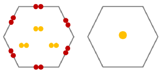
Figure 4: Schematic of degrees of freedom for velocity and pressure for WG method over the polygon.

Lemma 2.3.

(approximation properties). We have for $\bm{v}\in S_{h}$

$$\|\bm{v}-\Pi^{RT}\bm{v}\|_{0}\leq Ch\|\bm{v}\|_{h}.$$

Proof.

For any $T\in\mathcal{T}_{u}$, notice that $\bm{v}$ is a constant over the sub-triangle of $T$ and we use $\bm{v}_{i}$ to denote the value of $\bm{v}$ restricted to each sub-triangle $\tau\subset T$. Let $\bar{\bm{v}}=\frac{1}{|T|}\sum_{i=1}^{m}\int_{\tau}\bm{v}_{i}$ and we use $\|\bm{v}\|_{h,T}$ to represent $\|\bm{v}\|_{h}$ restricted to $T$, then we have

$$\|\bm{v}-\bar{\bm{v}}\|_{0,T}\leq Ch_{T}\|\bm{v}\|_{h,T},$$ (2.17)

where we use the fact that if the right side vanishes, then the left side also vanishes. An application of scaling arguments yields the desired estimate.

Since $\Pi^{RT}\bar{\bm{v}}=\bar{\bm{v}}$ for $\bar{\bm{v}}\in[P^{0}(T)]^{2}$, we can proceed analogously to (2.17) to obtain

$$\|\Pi^{RT}\bar{\bm{v}}-\Pi^{RT}\bm{v}\|_{0,T}=\|\sum_{i=1}^{m}(\bar{\bm{v}}-\bm{v}_{i})\bm{\varphi}_{i}\|_{0,T}\leq C\sum_{i=1}^{m}|\bar{\bm{v}}-\bm{v}_{i}|\|\bm{\varphi}_{i}\|_{0,T}\leq Ch_{T}\|\bm{v}\|_{h,T},$$

where Lemma 2.1 is employed in the last inequality.

Finally, the triangle inequality yields

$$\|\bm{v}-\Pi^{RT}\bm{v}\|_{0,T}\leq\|\bm{v}-\bar{\bm{v}}\|_{0,T}+\|\Pi^{RT}\bar{\bm{v}}-\Pi^{RT}\bm{v}\|_{0,T}.$$

Summing up over all the primal elements $T\in\mathcal{T}_{u}$ yields the desired estimate.

∎

3 A priori error analysis

In this section we will present the convergence estimates for all the variables involved. In particular we will prove that the error estimates for velocity are independent of $\nu$. The main contribution of this section is to prove the superconvergence of velocity via duality argument, which is non-trivial.

The unique solvability of the discrete formulation (2.5) can be proved in line with [56]. The proof will not be repeated here for the sake of conciseness. We will give the uniform a priori bound for velocity in the next lemma.

Lemma 3.1.

(uniform a priori bound on the discrete velocity). The following estimate holds

$$\|\bm{u}_{h}\|_{h}\leq C\nu^{-1}\|\bm{g}\|_{0}.$$ (3.1)

Proof.

Invoking (2.13) and (2.15), we can rewrite (2.5) as

$$B_{h}(\bm{\omega}_{h},\bm{v})+b_{h}^{*}(p_{h},\bm{v}) =(\bm{g},\Pi^{RT}\bm{v})+\lambda b_{h}^{*}(\pi_{h}\chi,\bm{v})\quad\forall\bm{v}\in S_{h},$$ (3.2)

$$B_{h}^{*}(\bm{u}_{h},\bm{\psi}) =\nu^{-1}(\bm{\omega}_{h},\bm{\psi})\hskip 68.28644pt\forall\bm{\psi}\in V_{h},$$ (3.3)

$$b_{h}(\bm{u}_{h},q) =0\hskip 113.81102pt\forall q\in M_{h}.$$ (3.4)

Taking $\bm{v}=\bm{u}_{h},\bm{\psi}=\bm{\omega}_{h},q=p_{h}-\lambda\pi_{h}\chi$ in (3.2), (3.3) and (3.4), and sum up, we can obtain

$$\nu^{-1}\|\bm{\omega}_{h}\|_{0}^{2}=(\bm{g},\Pi^{RT}\bm{u}_{h}).$$ (3.5)

We can infer from (2.6), (2.8) and (3.3) that

$$\|\bm{u}_{h}\|_{h}\leq C\sup_{\bm{\psi}\in V_{h}}\frac{B_{h}(\bm{\psi},\bm{u}_{h})}{\|\bm{\psi}\|_{0}}=C\sup_{\bm{\psi}\in V_{h}}\frac{B_{h}^{*}(\bm{u}_{h},\bm{\psi})}{\|\bm{\psi}\|_{0}}=C\sup_{\bm{\psi}\in V_{h}}\frac{\nu^{-1}(\bm{\omega}_{h},\bm{\psi})}{\|\bm{\psi}\|_{0}}\leq C\nu^{-1}\|\bm{\omega}_{h}\|_{0},$$

thereby, we can infer from Lemma 2.3 and (3.5)

$$\|\bm{u}_{h}\|_{h}^{2}\leq C\nu^{-2}\|\bm{\omega}_{h}\|_{0}^{2}\leq C\nu^{-1}\|\bm{g}\|_{0}\|\Pi^{RT}\bm{u}_{h}\|_{0}\leq C\nu^{-1}\|\bm{g}\|_{0}\|\bm{u}_{h}\|_{h},$$

which yields the desired estimate by dividing both sides by $\|\bm{u}_{h}\|_{h}$.

∎

Remark 3.1.

Contrary to the classical estimate $\|\bm{u}_{h}\|_{h}\leq C\nu^{-1}\|\bm{f}\|_{0}$ that can be obtained from [30] and [56], the a priori bound (3.1) persists in the limit $\lambda\rightarrow\infty$. This bound can be incorporated into Navier-Stokes equations to establish error estimates under smallness assumption that only concerns the solenoidal part $\bm{g}$ of the body force. This can improve the existing bound given in [15], where smallness assumption for $\bm{f}$ is required.

Theorem 3.1.

Let $(\bm{\omega},\bm{u},p)\in[H^{1}(\Omega)]^{2\times 2}\times[H^{1}(\Omega)]^{2}\times H^{1}(\Omega)$ be the weak solution of (2.2), $\Delta\bm{u}\in[L^{2}(\Omega)]^{2}$ and let $(\bm{\omega}_{h},\bm{u}_{h},p_{h})\in V_{h}\times S_{h}\times P_{h}$ be the numerical solution of (2.5). Then the following estimates hold

$$\|\bm{w}-\bm{w}_{h}\|_{0} \leq Ch(\nu\|\Delta\bm{u}\|_{0}+\|\bm{\omega}\|_{1}),$$

$$\|\mathcal{I}_{h}\bm{u}-\bm{u}_{h}\|_{h} \leq Ch(\|\bm{u}\|_{2}+\|\Delta\bm{u}\|_{0}),$$

$$\|p-p_{h}\|_{0} \leq Ch(\|p\|_{1}+\nu\|\Delta\bm{u}\|_{0}+\|\bm{\omega}\|_{1}).$$

Proof.

First, we define $\tilde{\bm{\omega}}\in V_{h}$ such that

$$\nu^{-1}(\tilde{\bm{\omega}},\bm{\psi})=B_{h}^{*}(\mathcal{I}_{h}\bm{u},\bm{\psi})\quad\forall\bm{\psi}\in V_{h}.$$ (3.6)

Invoking (2.5b) and (3.6), we can obtain

$$\nu^{-1}(\tilde{\bm{\omega}}-\bm{\omega}_{h},\bm{\psi})=B_{h}^{*}(\mathcal{I}_{h}\bm{u}-\bm{u}_{h},\bm{\psi})\quad\forall\bm{\psi}\in V_{h}.$$ (3.7)

We can infer from (2.10) and (3.6) that

$$\nu^{-1}(\tilde{\bm{\omega}},\bm{\psi})=B_{h}^{*}(\mathcal{I}_{h}\bm{u},\bm{\psi})=B_{h}^{*}(\bm{u},\bm{\psi})=\nu^{-1}(\bm{\omega},\bm{\psi})\quad\forall\bm{\psi}\in V_{h},$$

which means $\bm{\tilde{\omega}}$ is the $L^{2}$-orthogonal projection of $\bm{\omega}$ onto $V_{h}$. Thus,

$$\|\tilde{\bm{\omega}}-\bm{\omega}\|_{0}\leq\|\bm{\omega}-\mathcal{J}_{h}\bm{\omega}\|_{0}.$$

An appeal to (2.6), (2.8) and (3.7) yields

$$\|\mathcal{I}_{h}\bm{u}-\bm{u}_{h}\|_{h}\leq C\sup_{\bm{\psi}\in V_{h}}\frac{B_{h}(\bm{\psi},\mathcal{I}_{h}\bm{u}-\bm{u}_{h})}{\|\bm{\psi}\|_{0}}=C\sup_{\bm{\psi}\in V_{h}}\frac{B_{h}^{*}(\mathcal{I}_{h}\bm{u}-\bm{u}_{h},\bm{\psi})}{\|\bm{\psi}\|_{0}}\leq C\nu^{-1}\|\tilde{\bm{\omega}}-\bm{\omega}_{h}\|_{0}.$$ (3.8)

On the other hand, we can infer from the first equation of (1.1) and (2.16) that

$$(\bm{f},\Pi^{RT}\bm{v}) =(-\nu\Delta\bm{u}+\nabla p,\Pi^{RT}\bm{v})=-\nu(\Delta\bm{u},\Pi^{RT}\bm{v})+b_{h}^{*}(\pi_{h}p,\bm{v})\quad\forall\bm{v}\in S_{h}.$$

Integration by parts yields

$$B_{h}(\bm{w},\bm{v})=-(\bm{v},\nabla\cdot\bm{w})=-\nu(\bm{v},\Delta\bm{u})\quad\forall\bm{v}\in S_{h}.$$

Thereby, we can obtain

$$B_{h}(\bm{w},\bm{v})+b_{h}^{*}(\pi_{h}p,\bm{v})=(\bm{f},\Pi^{RT}\bm{v})+\nu(\Delta\bm{u},\Pi^{RT}\bm{v}-\bm{v})\quad\forall\bm{v}\in S_{h}.$$ (3.9)

On the other hand, we have from the discrete formulation (2.5a)

$$B_{h}(\bm{w}_{h},\bm{v})+b_{h}^{*}(p_{h},\bm{v})=(\bm{f},\Pi^{RT}\bm{v})\quad\forall\bm{v}\in S_{h},$$

which can be combined with (3.9) yielding

$$B_{h}(\bm{w}-\bm{w}_{h},\bm{v})+b_{h}^{*}(\pi_{h}p-p_{h},\bm{v})=(\nu\Delta\bm{u},\Pi^{RT}\bm{v}-\bm{v})\quad\forall\bm{v}\in S_{h}.$$

Hence

$$B_{h}(\mathcal{J}_{h}\bm{w}-\bm{w}_{h},\bm{v})+b_{h}^{*}(\pi_{h}p-p_{h},\bm{v})=\nu(\Delta\bm{u},\Pi^{RT}\bm{v}-\bm{v})\quad\forall\bm{v}\in S_{h}.$$ (3.10)

Taking $\bm{v}=\mathcal{I}_{h}\bm{u}-\bm{u}_{h}$ in (3.10), then it leads to

$$B_{h}(\mathcal{J}_{h}\bm{w}-\bm{w}_{h},\mathcal{I}_{h}\bm{u}-\bm{u}_{h})+b_{h}^{*}(\pi_{h}p-p_{h},\mathcal{I}_{h}\bm{u}-\bm{u}_{h})=\nu(\Delta\bm{u},\Pi^{RT}(\mathcal{I}_{h}\bm{u}-\bm{u}_{h})-(\mathcal{I}_{h}\bm{u}-\bm{u}_{h})).$$

Since $b_{h}^{*}(\pi_{h}p-p_{h},\mathcal{I}_{h}\bm{u}-\bm{u}_{h})=b_{h}(\mathcal{I}_{h}\bm{u}-\bm{u}_{h},\pi_{h}p-p_{h})=0$, we have

$$B_{h}(\bm{w}-\bm{w}_{h},\mathcal{I}_{h}\bm{u}-\bm{u}_{h})=\nu(\Delta\bm{u},\Pi^{RT}(\mathcal{I}_{h}\bm{u}-\bm{u}_{h})-(\mathcal{I}_{h}\bm{u}-\bm{u}_{h})).$$ (3.11)

It follows from (2.6), (2.11), (3.7) and (3.11) that

$$\begin{split}\nu^{-1}\|\tilde{\bm{\omega}}-\bm{\omega}_{h}\|_{0}^{2}&=B_{h}(\tilde{\bm{\omega}}-\bm{\omega}_{h},\mathcal{I}_{h}\bm{u}-\bm{u}_{h})\\ &=B_{h}(\tilde{\bm{\omega}}-\bm{\omega},\mathcal{I}_{h}\bm{u}-\bm{u}_{h})+\nu(\Delta\bm{u},\Pi^{RT}(\mathcal{I}_{h}\bm{u}-\bm{u}_{h})-(\mathcal{I}_{h}\bm{u}-\bm{u}_{h}))\\ &=B_{h}(\tilde{\bm{\omega}}-\mathcal{J}_{h}\bm{\omega},\mathcal{I}_{h}\bm{u}-\bm{u}_{h})+\nu(\Delta\bm{u},\Pi^{RT}(\mathcal{I}_{h}\bm{u}-\bm{u}_{h})-(\mathcal{I}_{h}\bm{u}-\bm{u}_{h})),\end{split}$$

therefore, we have from Lemma 2.3 and (3.8)

$$\|\tilde{\bm{\omega}}-\bm{\omega}_{h}\|_{0}^{2} \leq C\Big{(}\nu\|\tilde{\bm{\omega}}-\mathcal{J}_{h}\bm{\omega}\|_{0}\|\mathcal{I}_{h}\bm{u}-\bm{u}_{h}\|_{h}+\nu^{2}h\|\Delta\bm{u}\|_{0}\|\mathcal{I}_{h}\bm{u}-\bm{u}_{h}\|_{h}\Big{)}$$

$$\leq C\Big{(}\|\tilde{\bm{\omega}}-\mathcal{J}_{h}\bm{\omega}\|_{0}\|\tilde{\bm{\omega}}-\bm{\omega}_{h}\|_{0}+\nu h\|\Delta\bm{u}\|_{0}\|\tilde{\bm{\omega}}-\bm{\omega}_{h}\|_{0}\Big{)}.$$

The triangle inequality yields

$$\|\tilde{\bm{\omega}}-\mathcal{J}_{h}\bm{\omega}\|_{0}\leq\|\tilde{\bm{\omega}}-\bm{\omega}\|_{0}+\|\bm{\omega}-\mathcal{J}_{h}\bm{\omega}\|_{0}\leq 2\|\bm{\omega}-\mathcal{J}_{h}\bm{\omega}\|_{0}.$$

Thus, we can conclude that

$$\|\tilde{\bm{\omega}}-\bm{\omega}_{h}\|_{0}\leq Ch(\|\bm{\omega}\|_{1}+\nu\|\Delta\bm{u}\|_{0}),$$

which gives

$$\|\bm{\omega}-\bm{\omega}_{h}\|_{0}\leq Ch(\|\bm{\omega}\|_{1}+\nu\|\Delta\bm{u}\|_{0}).$$

Invoking (3.8), we can obtain

$$\|\mathcal{I}_{h}\bm{u}-\bm{u}_{h}\|_{h}\leq C\nu^{-1}\|\tilde{\bm{\omega}}-\bm{\omega}_{h}\|_{0}\leq Ch(\nu^{-1}\|\bm{\omega}\|_{1}+\|\Delta\bm{u}\|_{0})\leq Ch(\|\bm{u}\|_{2}+\|\Delta\bm{u}\|_{0}).$$ (3.12)

Next, we consider the error estimate for $\|p-p_{h}\|_{0}$. The discrete adjoint property (2.7) and the inf-sup condition (2.9) imply

$$\|p_{h}-\pi_{h}p\|_{0}\leq C\sup_{\bm{v}\in S_{h}\setminus\{0\}}\frac{b_{h}(\bm{v},p_{h}-\pi_{h}p)}{\|\bm{v}\|_{h}}=C\sup_{\bm{v}\in S_{h}\setminus\{0\}}\frac{b_{h}^{*}(p_{h}-\pi_{h}p,\bm{v})}{\|\bm{v}\|_{h}}.$$ (3.13)

Moreover, (3.10) yields

$$\begin{split}b_{h}^{*}(p_{h}-\pi_{h}p,\bm{v})&=B_{h}(\mathcal{J}_{h}\bm{\omega}-\bm{\omega}_{h},\bm{v})-\nu(\Delta\bm{u},\Pi^{RT}\bm{v}-\bm{v})\quad\forall\bm{v}\in S_{h}.\end{split}$$ (3.14)

We have from (2.4), Lemma 2.3, (3.13) and (3.14) that

$$\begin{split}\|p_{h}-\pi_{h}p\|_{0}&\leq C(\|\mathcal{J}_{h}\bm{\omega}-\bm{\omega}_{h}\|_{0}+\nu h\|\Delta\bm{u}\|_{0}).\end{split}$$

Therefore, we can obtain

$$\|p-p_{h}\|_{0} \leq C(\|p-\pi_{h}p\|_{0}+\|\bm{\omega}_{h}-\mathcal{J}_{h}\bm{\omega}\|_{0}+\nu h\|\Delta\bm{u}\|_{0})$$

$$\leq Ch(\|p\|_{1}+\|\bm{\omega}\|_{1}+\nu\|\Delta\bm{u}\|_{0}).$$

∎

The $L^{2}$ error estimate for velocity can be stated as follows.

Theorem 3.2.

Let $(\bm{\omega},\bm{u})\in[H^{1}(\Omega)]^{2\times 2}\times[H^{1}(\Omega)]^{2}$ be the weak solution of (2.2) and $\Delta\bm{u}\in[L^{2}(\Omega)]^{2}$, and let $\bm{u}_{h}\in S_{h}$ be the numerical solution of (2.5). Then the following estimate holds

$$\|\bm{u}-\bm{u}_{h}\|_{0}\leq Ch\Big{(}\|\Delta\bm{u}\|_{0}+\|\bm{u}\|_{2}\Big{)}.$$

Proof.

We have from the discrete Poincaré inequality (cf. [6]) and (3.12) that

$$\|\mathcal{I}_{h}\bm{u}-\bm{u}_{h}\|_{0}\leq C\|\mathcal{I}_{h}\bm{u}-\bm{u}_{h}\|_{h}\leq Ch(\|\bm{u}\|_{2}+\|\Delta\bm{u}\|_{0}).$$

Then we can infer from the triangle inequality and (2.12)

$$\|\bm{u}-\bm{u}_{h}\|_{0}\leq\|\mathcal{I}_{h}\bm{u}-\bm{u}\|_{0}+\|\mathcal{I}_{h}\bm{u}-\bm{u}_{h}\|_{0}\leq Ch\Big{(}\|\bm{u}\|_{2}+\|\Delta\bm{u}\|_{0}\Big{)}.$$

∎

Now we state the superconvergence for velocity.

Theorem 3.3.

(superconvergence). Let $(\bm{\omega},\bm{u})\in[H^{1}(\Omega)]^{2\times 2}\times[H^{1}(\Omega)]^{2}$ be the weak solution of (2.2), $\Delta\bm{u}\in[H^{2}(\Omega)]^{2}$ and let $\bm{u}_{h}\in S_{h}$ be the numerical solution of (2.5). Then the following estimate holds

$$\|\mathcal{I}_{h}\bm{u}-\bm{u}_{h}\|_{0}\leq Ch^{2}(\|\bm{u}\|_{2}+\|\Delta\bm{u}\|_{2}).$$

Proof.

Given a right hand side $\bm{r}\in[L^{2}(\Omega)]^{2}$, let $(\bm{\omega}_{r},\bm{u}_{r},p_{r})$ denote the solution of

$$\nabla\cdot\bm{\omega}_{r}+\nabla p_{r} =\bm{r}\hskip 34.14322pt\mbox{in}\;\Omega,$$ (3.15)

$$\bm{\omega}_{r} =-\nu\nabla\bm{u}_{r}\quad\mbox{in}\;\Omega,$$ (3.16)

$$\nabla\cdot\bm{u}_{r} =0\hskip 36.98866pt\mbox{in}\;\Omega,$$ (3.17)

$$\bm{u}_{r} =\bm{0}\hskip 36.98866pt\mbox{on}\;\partial\Omega$$ (3.18)

and let $(\bm{\omega}_{r,h},\bm{u}_{r,h},p_{r,h})\in V_{h}\times S_{h}\times P_{h}$ denote the solution of

$$-B_{h}(\bm{\omega}_{r,h},\bm{v})+b_{h}^{*}(p_{r,h},\bm{v}) =(\bm{r},\Pi^{RT}\bm{v})\qquad\forall\bm{v}\in S_{h},$$ (3.19)

$$-B_{h}^{*}(\bm{u}_{r,h},\bm{\psi}) =\nu^{-1}(\bm{\omega}_{r,h},\bm{\psi})\quad\forall\bm{\psi}\in V_{h},$$ (3.20)

$$b_{h}(\bm{u}_{r,h},q)= 0\hskip 71.13188pt\forall q\in P_{h}.$$ (3.21)

We obtain from classical regularity results for the incompressible Stokes equations (cf. [25]) that

$$\begin{split}\nu\|\bm{u}_{r}\|_{2}&\leq C\|\bm{r}\|_{0},\\ \|\bm{\omega}_{r}\|_{1}&\leq C\|\bm{r}\|_{0}.\end{split}$$ (3.22)

We can now apply a duality argument to prove the superconvergence. We have

$$\|\mathcal{I}_{h}\bm{u}-\bm{u}_{h}\|_{0}=\sup_{\bm{r}\in[L^{2}(\Omega)]^{2}\backslash\{\bm{0}\}}\frac{(\bm{r},\mathcal{I}_{h}\bm{u}-\bm{u}_{h})}{\|\bm{r}\|_{0}}$$

and

$$(\bm{r},\mathcal{I}_{h}\bm{u}-\bm{u}_{h}) =(\bm{r},\mathcal{I}_{h}\bm{u}-\bm{u}_{h}-\Pi^{RT}(\mathcal{I}_{h}\bm{u}-\bm{u}_{h}))+(\bm{r},\Pi^{RT}(\mathcal{I}_{h}\bm{u}-\bm{u}_{h})).$$ (3.23)

The first term on the right hand side can be estimated by Lemma 2.3 and (3.12)

$$(\bm{r},\mathcal{I}_{h}\bm{u}-\bm{u}_{h}-\Pi^{RT}(\mathcal{I}_{h}\bm{u}-\bm{u}_{h}))\leq Ch\|\bm{r}\|_{0}\|\mathcal{I}_{h}\bm{u}-\bm{u}_{h}\|_{h}\leq Ch^{2}\|\bm{r}\|_{0}(\|\Delta\bm{u}\|_{0}+\|\bm{u}\|_{2}).$$

It remains to estimate the second term of (3.23). We have from (3.16), (3.19), integration by parts and the fact that $b_{h}^{*}(p_{r,h},\mathcal{I}_{h}\bm{u}-\bm{u}_{h})=0$

$$\begin{split}(\bm{r},\Pi^{RT}(\mathcal{I}_{h}\bm{u}-\bm{u}_{h}))&=-B_{h}(\bm{\omega}_{r,h},\mathcal{I}_{h}\bm{u}-\bm{u}_{h})+\nu^{-1}(\bm{\omega}_{r},\bm{\omega}-\bm{\omega}_{h})+(\nabla\bm{u}_{r},\bm{\omega}-\bm{\omega}_{h})\\ &=-B_{h}(\bm{\omega}_{r,h},\mathcal{I}_{h}\bm{u}-\bm{u}_{h})+\nu^{-1}(\bm{\omega}_{r},\bm{\omega}-\bm{\omega}_{h})+(\nabla(\bm{u}_{r}-\mathcal{I}_{h}\bm{u}_{r}),\bm{\omega}-\bm{\omega}_{h})\\ &=-B_{h}(\bm{\omega}_{r,h},\mathcal{I}_{h}\bm{u}-\bm{u}_{h})+\nu^{-1}(\bm{\omega}_{r},\bm{\omega}-\bm{\omega}_{h})+\sum_{e\in\mathcal{F}_{p}}((\bm{\omega}-\bm{\omega}_{h})\bm{n},[\bm{u}_{r}-\mathcal{I}_{h}\bm{u}_{r}])_{e}\\ &\;+\sum_{e\in\mathcal{F}_{u}}([(\bm{\omega}-\bm{\omega}_{h})\bm{n}],\bm{u}_{r}-\mathcal{I}_{h}\bm{u}_{r})_{e}-(\bm{u}_{r}-\mathcal{I}_{h}\bm{u}_{r},\nabla\cdot\bm{\omega})\\ &=-B_{h}(\bm{\omega}_{r,h},\mathcal{I}_{h}\bm{u}-\bm{u}_{h})+\nu^{-1}(\bm{\omega}_{r},\bm{\omega}-\bm{\omega}_{h})\\ &\;+B_{h}(\bm{\omega}-\bm{\omega}_{h},\mathcal{I}_{h}\bm{u}_{r})-(\bm{u}_{r}-\mathcal{I}_{h}\bm{u}_{r},\nabla\cdot\bm{\omega}).\end{split}$$ (3.24)

It follows from (2.5b) and (3.10) by taking $\bm{\psi}=\mathcal{J}_{h}\bm{\omega}_{r}$ and $\bm{v}=\mathcal{I}_{h}\bm{u}_{r}$, respectively

$$B_{h}^{*}(\mathcal{I}_{h}\bm{u}-\bm{u}_{h},\mathcal{J}_{h}\bm{\omega}_{r}) =\nu^{-1}(\bm{\omega}-\bm{\omega}_{h},\mathcal{J}_{h}\bm{\omega}_{r}),$$

$$B_{h}(\bm{\omega}-\bm{\omega}_{h},\mathcal{I}_{h}\bm{u}_{r}) =\nu(\Delta\bm{u},\Pi^{RT}\mathcal{I}_{h}\bm{u}_{r}-\mathcal{I}_{h}\bm{u}_{r}),$$

where we use $b_{h}^{*}(\pi_{h}p-p_{h},\mathcal{I}_{h}\bm{u}_{r})=0$ in the second equality.

Therefore, we can recast (3.24) into the following form

$$(\bm{r},\Pi^{RT}(\mathcal{I}_{h}\bm{u}-\bm{u}_{h})) =-B_{h}(\bm{\omega}_{r,h}-\mathcal{J}_{h}\bm{\omega}_{r},\mathcal{I}_{h}\bm{u}-\bm{u}_{h})+\nu^{-1}(\bm{\omega}_{r}-\mathcal{J}_{h}\bm{\omega}_{r},\bm{\omega}-\bm{\omega}_{h})$$

$$\;+\nu(\Delta\bm{u},\Pi^{RT}\mathcal{I}_{h}\bm{u}_{r}-\mathcal{I}_{h}\bm{u}_{r})-(\bm{u}_{r}-\mathcal{I}_{h}\bm{u}_{r},\nabla\cdot\bm{\omega})$$

$$=-B_{h}(\bm{\omega}_{r,h}-\mathcal{J}_{h}\bm{\omega}_{r},\mathcal{I}_{h}\bm{u}-\bm{u}_{h})+\nu^{-1}(\bm{\omega}_{r}-\mathcal{J}_{h}\bm{\omega}_{r},\bm{\omega}-\bm{\omega}_{h})$$

$$\;+\nu(\Delta\bm{u},\Pi^{RT}\mathcal{I}_{h}\bm{u}_{r}-\mathcal{I}_{h}\bm{u}_{r})-\nu(\Delta\bm{u},\bm{u}_{r}-\mathcal{I}_{h}\bm{u}_{r})$$

$$=-B_{h}(\bm{\omega}_{r,h}-\mathcal{J}_{h}\bm{\omega}_{r},\mathcal{I}_{h}\bm{u}-\bm{u}_{h})+\nu^{-1}(\bm{\omega}_{r}-\mathcal{J}_{h}\bm{\omega}_{r},\bm{\omega}-\bm{\omega}_{h})+\nu(\Delta\bm{u},\Pi^{RT}\mathcal{I}_{h}\bm{u}_{r}-\bm{u}_{r})$$

$$:=\sum_{i=1}^{3}I_{i}.$$

First we can obtain the following estimate by proceeding analogously to Theorem 3.1 for the dual problem (3.15)-(3.21)

$$\|\bm{\omega}_{r,h}-\mathcal{J}_{h}\bm{\omega}_{r}\|_{0}\leq C\Big{(}\|\bm{\omega}_{r}-\mathcal{J}_{h}\bm{\omega}_{r}\|_{0}+\nu h\|\Delta\bm{u}_{r}\|_{0}\Big{)}\leq Ch\Big{(}\|\bm{\omega}_{r}\|_{1}+\nu\|\Delta\bm{u}_{r}\|_{0}\Big{)}\leq Ch\|\bm{r}\|_{0}.$$ (3.25)

Then $I_{1}$ can be estimated by the Cauchy-Schwarz inequality, (3.12) and (3.25)

$$|I_{1}|\leq C\|\bm{\omega}_{r,h}-\mathcal{J}_{h}\bm{\omega}_{r}\|_{0}\|\mathcal{I}_{h}\bm{u}-\bm{u}_{h}\|_{h}\leq h^{2}\|\bm{r}\|_{0}(\|\Delta\bm{u}\|_{0}+\|\bm{u}\|_{2}).$$

We can bound $I_{2}$ by the Cauchy-Schwarz inequality and Theorem 3.1

$$|I_{2}|\leq\nu^{-1}\|\bm{\omega}_{r}-\mathcal{J}_{h}\bm{\omega}_{r}\|_{0}\|\bm{\omega}-\bm{\omega}_{h}\|_{0}\leq C\nu^{-1}h^{2}\|\bm{w}_{r}\|_{1}(\nu\|\Delta\bm{u}\|_{0}+\|\bm{\omega}\|_{1})\leq Ch^{2}\|\bm{r}\|_{0}(\|\Delta\bm{u}\|_{0}+\nu^{-1}\|\bm{\omega}\|_{1}).$$

For an arbitrary $T\in\mathcal{T}_{u}$ with $m$ edges, we have from the definitions of $\Pi^{RT}$ and $\mathcal{I}_{h}$

$$\Pi^{RT}\mathcal{I}_{h}\bm{u}_{r}=\sum_{i=1}^{m}(\frac{1}{|e|}\int_{e}\mathcal{I}_{h}\bm{u}_{r}\cdot\bm{n}\;ds)\bm{\varphi}_{i}=\sum_{i=1}^{m}(\frac{1}{|e|}\int_{e}\bm{u}_{r}\cdot\bm{n}\;ds)\bm{\varphi}_{i}.$$

Thus, we can conclude that $\Pi^{RT}\mathcal{I}_{h}\bm{u}_{r}=\Pi^{RT}\bm{u}_{r}$. Thereby we can rewrite $I_{3}$ as

$$I_{3} =\nu(\Delta\bm{u},\Pi^{RT}\mathcal{I}_{h}\bm{u}_{r}-\bm{u}_{r})=\nu(\Delta\bm{u},\Pi^{RT}\bm{u}_{r}-\bm{u}_{r})$$

$$=\nu(\Delta\bm{u}-\pi_{h}\Delta\bm{u},\Pi^{RT}\bm{u}_{r}-\bm{u}_{r})+\nu(\pi_{h}\Delta\bm{u},\Pi^{RT}\bm{u}_{r}-\bm{u}_{r}).$$

For the first summand, Lemma 2.1 and (3.22) give the desired bound

$$\nu(\Delta\bm{u}-\pi_{h}\Delta\bm{u},\Pi^{RT}\bm{u}_{r}-\bm{u}_{r}) \leq\nu\|\Delta\bm{u}-\pi_{h}\Delta\bm{u}\|_{0}\|\Pi^{RT}\bm{u}_{r}-\bm{u}_{r}\|_{0}$$

$$\leq C\nu h^{2}\|\Delta\bm{u}\|_{1}\|\bm{u}_{r}\|_{1}\leq Ch^{2}\|\Delta\bm{u}\|_{1}\|\bm{r}\|_{0}.$$

The bound for the second summand is inspired by the work given in [37]. First, we notice that $\nabla\cdot\bm{u}_{r}=0$, hence there exists a function $\sigma_{r}$ such that $\text{curl}\,\sigma_{r}=\bm{u}_{r}$. Further, since $\bm{u}_{r}\in[H^{1}(\Omega)]^{2}$, it holds $\nu\|\sigma_{r}\|_{2}\leq C\|\bm{r}\|_{0}$, see, e.g., [28]. Furthermore, there exists a space $\widetilde{S}_{h}$ consisting of piecewise linear polynomials and recall that $\Pi^{0}$ is the nodal value interpolation operator based on the generalized barycentric coordinates (cf. Lemma 2.1). Since $\Pi^{RT}$ satisfies (2.3), it holds $\bm{u}_{r}-\Pi^{RT}\bm{u}_{r}=\text{curl}(\sigma_{r}-\Pi^{0}\sigma_{r})$

$$\nu(\pi_{h}\Delta\bm{u},\bm{u}_{r}-\Pi^{RT}\bm{u}_{r}) =\nu\sum_{T\in\mathcal{T}_{u}}(\pi_{h}\Delta\bm{u},\text{curl}(\sigma_{r}-\Pi^{0}\sigma_{r}))_{T}$$

$$\leq|\sum_{T\in\mathcal{T}_{u}}\nu(\text{curl}(\pi_{h}\Delta\bm{u}),\sigma_{r}-\Pi^{0}\sigma_{r})_{T}|+\nu|\sum_{T\in\mathcal{T}_{u}}(\pi_{h}\Delta\bm{u}\cdot\bm{t},\sigma_{r}-\Pi^{0}\sigma_{r})_{\partial T}|$$

The first term on the right hand side vanishes since $\pi_{h}\Delta\bm{u}$ is piecewise constant. We can bound the second term by the error estimates on convex polygon based on the generalized barycentric coordinates (cf. [24])

$$|(\pi_{h}\Delta\bm{u}\cdot\bm{t},\sigma_{r}-\Pi^{0}\sigma_{r})_{\partial T}| \leq\|\pi_{h}\Delta\bm{u}\|_{L^{\infty}(\partial T)}\|\sigma_{r}-\Pi^{0}\sigma_{r}\|_{L^{1}(\partial T)}\leq Ch_{T}^{2}\|\Delta\bm{u}\|_{L^{\infty}(\partial T)}\|\sigma_{r}\|_{2,T}.$$

Thus

$$\nu(\pi_{h}\Delta\bm{u},\bm{u}_{r}-\Pi^{RT}\bm{u}_{r})\leq C\nu h^{2}\sum_{T\in\mathcal{T}_{u}}\|\Delta\bm{u}\|_{2,T}\|\sigma_{r}\|_{2,T}\leq Ch^{2}\|\Delta\bm{u}\|_{2}\|\bm{r}\|_{0}.$$

Combining the preceding arguments, we can achieve the desired estimate.

∎

Remark 3.2.

The derivation of superconvergence for lowest order SDG method is non-trivial. In general we need to invoke some nonstandard trace inequalities in order to deliver the desirable results, see [56]. Here, we are able to achieve the superconvergence without resorting to nonstandard trace inequality and the key idea lies in the use of the divergence preserving operator in the discrete formulation of the dual problem as well as the integration of continuous formulation and discrete formulation in (3.24). We emphasize that the sole application of continuous formulation (cf. (3.15)-(3.18)) or discrete formulation (cf. (3.19)-(3.21)) can not deliver desirable result. Importantly, our analysis will provide new perspectives for the proof of superconvergence for other discretizations as well.

Remark 3.3.

We can obtain the following estimate by using the formulation given in [56]

$$\|\bm{\omega}-\bm{\omega}_{h}\|_{0} \leq Ch(\nu\|\bm{u}\|_{2}+\|p\|_{1}),$$

$$\|\mathcal{I}_{h}\bm{u}-\bm{u}_{h}\|_{h} \leq Ch(\|\bm{u}\|_{2}+\frac{1}{\nu}\|p\|_{1}),$$

$$\|p-p_{h}\|_{0} \leq Ch(\nu\|\bm{u}\|_{2}+\|p\|_{1}).$$

Then the discrete Poincaré inequality (cf. [6]) yields

$$\|\mathcal{I}_{h}\bm{u}-\bm{u}_{h}\|_{0}\leq C\|\mathcal{I}_{h}\bm{u}-\bm{u}_{h}\|_{h}\leq Ch(\|\bm{u}\|_{2}+\frac{1}{\nu}\|p\|_{1}).$$

We can observe from the above estimates that the velocity error will grow unboundedly as $\nu\rightarrow 0$, and therefore the formulation from [56] generates unsatisfactory solution as $\nu\rightarrow 0$.

4 Numerical experiments

In this section several numerical tests will be tested to confirm the proposed theories. In the following tests, we will employ three types of meshes: Unstructured triangular mesh, trapezoidal mesh and polygonal mesh shown in Figure 5. The accuracy and robustness of the proposed method will be investigated. For the sake of simplicity we denote the present formulation (cf. (2.5)) as SDG1 and the formulation obtained from [56] as SDG2.

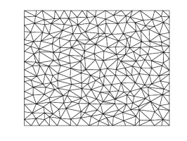
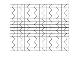
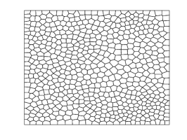
Figure 5: Three types of meshes used in numerical experiments: Unstructured triangular mesh (left), trapezoidal mesh (middle), and polygonal mesh (right).

4.1 Unstructured triangular mesh

4.1.1 Accuracy and robustness test

Let $\Omega=(0,1)^{2}$ and let the exact solution be given by

$$\bm{u}=\left(\begin{array}[]{c}\pi x^{2}(1-x)^{2}\sin(2\pi y)+1\\ -2x(1-x)(1-2x)\sin(\pi y)^{2}+1\\ \end{array}\right),\quad p=\sin(x)\cos(y)+(\cos(1)-1)\sin(1).$$ (4.3)

We use unstructured triangular meshes in this section for the numerical simulation, see Figure 5. The convergence history against the mesh size for $\nu=1$ are plotted in Figure 6. We can observe that first order convergence can be achieved in $L^{2}$ errors of $\bm{u},p$ and $\bm{\omega}$ for both algorithms; in addition, second order convergence can be obtained for $\|\mathcal{I}_{h}\bm{u}-\bm{u}_{h}\|_{0}$, which confirms the theoretical results presented in Theorem 3.1 and Theorem 3.3.

Then we perform simulations to test the robustness of our method. To this end, we fix $h=1/16$ and choose $\nu=10^{2},10,1,10^{-1},10^{-2},10^{-3},10^{-4},10^{-5},10^{-6}$. The right hand side can be calculated by $\bm{f}=-\nu\Delta\bm{u}+\nabla p$. $L^{2}$ errors for velocity, pressure and velocity gradient are reported in Figure 7. The velocity error deteriorates for $\nu\rightarrow 0$ and is asymptotically proportional to $1/\nu$ (when $\nu\leq 1$) as predicted by the theory of SDG2 (cf. Remark 3.3), which indicates that SDG2 is not pressure robust. On the contrary, the velocity error of SDG1 remains a constant for various values of $\nu$, which validates the independence of velocity on the pressure variable. In addition, we can observe similar performances for pressure error from SDG1 and SDG2. Moreover, the $L^{2}$ error of velocity gradient from SDG1 is asymptotically proportional to $\nu$, whereas, the $L^{2}$ error of velocity gradient from SDG2 tends to be a constant when $\nu\leq 1$, which is consistent with the theories given in Theorem 3.1 and Remark 3.3.

Finally, we display the numerical approximations for $\nu=10^{-6}$ for both algorithms in Figure 8. It is easy to see that SDG1 yields correct numerical approximation for velocity while SDG2 yields wrong numerical approximation for velocity. Numerical approximation for pressure is correct for both algorithms. To further verify the robustness of SDG1, we show the convergence history for $\nu=10^{-6}$, and we can observe first order convergence in $L^{2}$ errors of velocity, pressure and velocity gradient; in addition, superconvergence can be obtained for $\|\mathcal{I}_{h}\bm{u}-\bm{u}_{h}\|_{0}$.

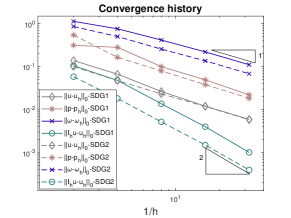
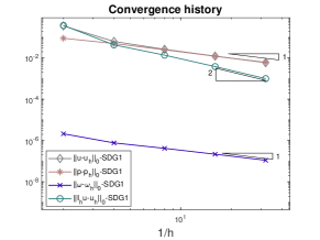
Figure 6: Example 4.1.1: Convergence history for $\nu=1$ (left) and $\nu=10^{-6}$ (right).

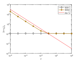
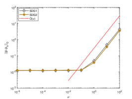
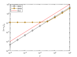
Figure 7: Example 4.1.1: Error profiles for velocity (left), pressure (middle) and velocity gradient (right) on unstructured triangular mesh with $h=1/16$.

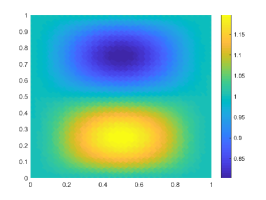
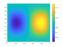
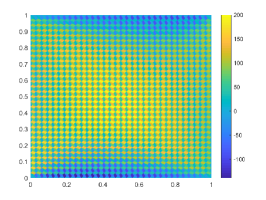
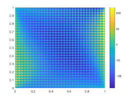
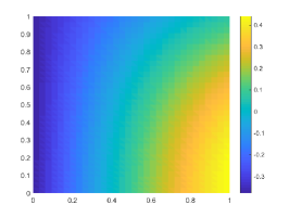
Figure 8: Example 4.1.1: Numerical approximations on the mesh with $h=1/32$ with $\nu=10^{-6}$. Top: numerical solution of $u_{1}$ (left), $u_{2}$ (middle), and $p$ (right) from SDG1. Bottom: numerical solution of $u_{1}$ (left), $u_{2}$ (middle), and $p$ (right) from SDG2.

4.1.2 No flow

In this example, we again set $\Omega=(0,1)^{2}$, and the exact velocity and pressure are defined by

$$\bm{u}=\left(\begin{array}[]{c}0\\ 0\\ \end{array}\right),\quad p=-\frac{\text{Ra}}{2}y^{2}+\text{Ra}y-\frac{\text{Ra}}{3},$$

where $\text{Ra}=1000$.

The numerical solution for velocity and pressure for both algorithms are displayed in Figure 9. We can observe that SDG1 delivers zero velocity fields, which matches the exact solution. However, SDG2 yields nonzero velocity, which is far from the exact velocity. Then we show the error profiles for $\|\bm{u}-\bm{u}_{h}\|_{0}$, $\|\bm{\omega}-\bm{\omega}_{h}\|_{0}$, $\|p-p_{h}\|_{0}$ and $\|\mathcal{I}_{h}\bm{u}-\bm{u}_{h}\|_{0}$. The errors from SDG1 approach zero, see Table 1, whereas this is not the case for SDG2, see Table 2.

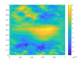
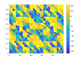
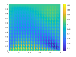
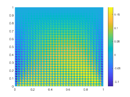
Figure 9: Example 4.1.2: Numerical approximations on the mesh with $h=1/32$. Top: numerical solution of $u_{1}$ (left), $u_{2}$ (middle), and $p$ (right) from SDG1. Bottom: numerical solution of $u_{1}$ (left), $u_{2}$ (middle), and $p$ (right) from SDG2.

Mesh	$\|\bm{u}-\bm{u}_{h}\|_{0}$		$\|\bm{\omega}-\bm{\omega}_{h}\|_{0}$		$\|p-p_{h}\|_{0}$		$\|\mathcal{I}_{h}\bm{u}-\bm{u}_{h}\|_{0}$
$h^{-1}$	Error	Order	Error	Order	Error	Order	Error	Order
2	1.94e-015	N/A	1.36e-014	N/A	66	N/A	1.94e-15	N/A
4	5.34e-016	1.86	5.00e-015	1.44	33	0.97	5.35e-16	1.86
8	3.95e-016	0.43	5.76e-015	-0.20	16	0.99	3.95e-16	0.43
16	3.73e-016	0.08	7.42e-015	-0.36	8.4	0.99	3.73e-16	0.08
32	2.63e-016	0.50	7.14e-015	0.05	4.2	0.99	2.63e-16	0.50

Table 1: Convergence history for SDG1 for Example 4.1.2.

Mesh	$\|\bm{u}-\bm{u}_{h}\|_{0}$		$\|\bm{\omega}-\bm{\omega}_{h}\|_{0}$		$\|p-p_{h}\|_{0}$		$\|\mathcal{I}_{h}\bm{u}-\bm{u}_{h}\|_{0}$
$h^{-1}$	Error	Order	Error	Order	Error	Order	Error	Order
2	8.75	N/A	51	N/A	75	N/A	8.75	N/A
4	3.60	1.27	34	0.57	38	0.95	3.60	1.27
8	1.12	1.68	19	0.83	18	1.05	1.12	1.68
16	0.30	1.88	10	0.93	8.9	1.06	0.30	1.88
32	0.08	1.95	5	0.97	4.3	1.04	0.07	1.96

Table 2: Convergence history for SDG2 for Example 4.1.2.

4.2 Trapezoidal mesh

Let $\Omega=(0,1)^{2}$ and we choose the exact solution to be

$$\bm{u}=\left(\begin{array}[]{c}-e^{x}(y\cos(y)+\sin(y))\\ e^{x}y\sin(y)\\ \end{array}\right),\quad p=2e^{x}\sin(y).$$

In this test, we employ the trapezoidal mesh shown in Figure 5. The convergence history against the number of degrees of freedom for $\nu=1$ is reported in Figure 10, and optimal convergence rates matching the theoretical results can be obtained. Moreover, we also show the convergence history against the number of degrees of freedom for $\nu=10^{-6}$ for SDG1, as expected, optimal convergence rates can be obtained. To verify the robustness, we show the errors for various values of $\nu$, i.e., $\nu=10^{j}(j=-6,\cdots,2)$ for both algorithms with the number of degrees of freedom (dof) to be $4993$ in Figure 11. Similarly, we can observe that SDG2 is not pressure robust and SDG1 is pressure robust. The velocity error of SDG1 remains a constant for various values of $\nu$ while the velocity error of SDG2 is asymptotically proportional to $1/\nu$ when $\nu\leq 1$. Moreover, the $L^{2}$ error of velocity gradient from SDG1 is asymptotically proportional to $\nu$, whereas, the $L^{2}$ error of velocity gradient from SDG2 tends to be a constant when $\nu\leq 1$.

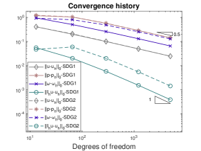
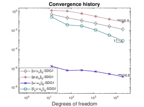
Figure 10: Example 4.2: Convergence history for $\nu=1$ (left) and $\nu=10^{-6}$ (right).

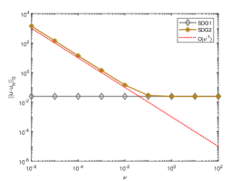
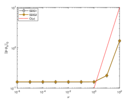
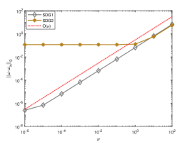
Figure 11: Example 4.2: Error profiles for velocity (left), pressure (middle) and velocity gradient (right) on trapezoidal mesh with $\text{dof}=4993$.

4.3 Polygonal mesh

In this example, we choose the same exact solution given in (4.3) and exploit the polygonal mesh displayed in Figure 5. Figure 12 shows the convergence history against the number of degrees of freedom for $\nu=1$. To verify the robustness of our method, we consider $L^{2}$ errors of velocity, pressure and velocity gradient with various values of $\nu$, i.e., $\nu=10^{j}(j=-5,\cdots,2)$ on the fixed mesh, and the numerical results are given in Figure 13. Again, we can obtain similar conclusions as sections 4.1 and 4.2.

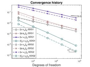
Figure 12: Example 4.3: Convergence history for $\nu=1$.

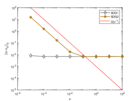
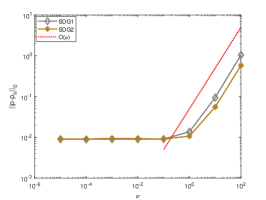
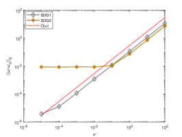
Figure 13: Example 4.3: Error profiles for velocity (left), pressure (middle) and velocity gradient (right) on polygonal mesh with $\text{dof}=4235$.

5 Conclusion

In this paper we have developed a pressure robust staggered discontinuous Galerkin method for the Stokes equations, where the crux is to modify the right hand side by using divergence preserving operator. It is proved theoretically that the velocity error estimates are independent of $\nu$. In addition, we are able to show that the numerical approximation for velocity superconverges to a suitable projection. Several numerical experiments are carried out to test the accuracy and robustness of the proposed method. In the future we will extend this approach to solve Navier-Stokes equations with arbitrary polynomial orders, in which case the smallness assumption given in [15] can be weakened to concern only the solenoidal part $\bm{g}$ of the body force.

References

- [1] D. Arnold, Finite Element Exterior Calculus, SIAM, Philadelphia, PA, 2018.
- [2] I. Babuška and M. Suri, On locking and robustness in the finite element method, ESAIM Math. Model. Numer. Anal., 29 (1992), pp. 1261–1293.
- [3] L. Beirão da Veiga, F. Brezzi, A. Cangiani, G. Manzini, L. D. Marini, and A. Russo, Basic principles of virtual element methods, Math. Models Meth. Appl. Sci., 23 (2013), pp. 199–214.
- [4] L. Beirão da Veiga, F. Brezzi, L. D. Marini and A. Russo, The hitchhiker’s guide to the virtual element method, Math. Models Meth. Appl. Sci., 24 (2014), pp. 1541–1573.
- [5] C. Brennecke, A. Linke, C. Merdon, and J. Schöberl, Optimal and pressure-independent L2 velocity error estimates for a modified Crouzeix-Raviart Stokes element with BDM reconstructions, J. Comput. Math., 33 (2015), pp. 191–208.
- [6] S. C. Brenner, Poincaré-Friedrichs inequalities for piecewise functions, SIAM J. Numer. Anal., 41 (2003), pp. 306–324.
- [7] W. Chen AND Y. Wang, Minimal degree and conforming finite elements on polytopal meshes, Math. Comp., 307 (2017), pp. pp. 2053–2087.
- [8] L. Chen and F. Wang, A divergence free weak virtual element method for the Stokes problem on polytopal meshes, J. Sci. Comput., 78 (2019), pp. 864–886.
- [9] S. W. Cheung, E. T. Chung, H. H. Kim and Y. Qian, Staggered discontinuous Galerkin methods for the incompressible Navier-Stokes equations, J. Comput. Phys., 302 (2015), pp. 251–266.
- [10] E. T. Chung, B. Cockburn and G. Fu, The staggered DG method is the limit of a hybridizable DG method, SIAM J. Numer. Anal., 52 (2014), pp. 915–932.
- [11] E. T. Chung, B. Cockburn and G. Fu, The staggered DG method is the limit of a hybridizable DG method. Part II: The Stokes flow, J. Sci. Comput., 66 (2016), pp. 870–887.
- [12] E. T. Chung and B. Engquist, Optimal discontinuous Galerkin methods for wave propagation, SIAM J. Numer. Anal., 44 (2006), pp. 2131–2158.
- [13] E. T. Chung and B. Engquist, Optimal discontinuous Galerkin methods for the acoustic wave equation in higher dimensions, SIAM J. Numer. Anal., 47 (2009), pp. 3820–3848.
- [14] E. T. Chung and C. S. Lee, A staggered discontinuous Galerkin method for the curl-curl operator, IMA J. Numer. Anal., 32 (2012), pp. 1241–1265.
- [15] E. T. Chung and W. Qiu, Analysis of an SDG method for the incompressible Navier-Stokes equations, SIAM J. Numer. Anal., 55 (2017), pp. 543–569.
- [16] P. G. Ciarlet, The Finite Element Method for Elliptic Problems, North-Holland Publishing, Amsterdam, 1978.
- [17] B. Cockburn, G. Kanschat, and D. Schötzau, A note on discontinuous Galerkin divergence-free solutions of the Navier-Stokes equations, J. Sci. Comput., 31 (2007), pp. 61–73.
- [18] D. A. Di Pietro and J. Droniou, The Hybrid High-Order method for polytopal meshes, No. 19 in Modeling, Simulation and Applications, Springer International Publishing, 2020.
- [19] D. A. Di Pietro, A. Ern, and S. Lemaire, An arbitrary-order and compact-stencil discretization of diffusion on general meshes based on local reconstruction operators, Comput. Methods Appl. Math., 14 (2014), pp. 461–472,
- [20] D. A. Di Pietro, A. Ern, A. Linke, and F. Schieweck, A discontinuous skeletal method for the viscosity-dependent Stokes problem, Comput. Methods Appl. Mech. Engrg., 306 (2016), pp. 175–195.
- [21] J. Du, E. T. Chung, M. F. Lam and X.-P. Wang, Discontinuous Galerkin method with staggered hybridization for a class of nonlinear Stokes equations, J. Sci. Comput., 76 (2018), pp. 1547–1577.
- [22] R. Falk and M. Neilan, Stokes complexes and the construction of stable finite elements with pointwise mass conservation, SIAM J. Numer. Anal., 51 (2013), pp. 1308–1326.
- [23] M. Floater, A. Gillette, and N. Sukumar, Gradient bounds for Wachspress coordinates on polytopes, SIAM J. Numer. Anal., 52 (2014), pp. 515–532.
- [24] A. Gillette, A. Rand, and C. Bajaj, Error estimates for generalized barycentric interpolation, Adv. Comput. Math., 37 (2012), pp. 417–439.
- [25] V. Girault and P.-A Raviart, Finite Element Methods for Navier–Stokes Equations, Springer Series in Computational Mathematics, vol. 5, Springer-Verlag, Berlin (1986) Theory and algorithms.
- [26] J. Guzmán and M. Neilan, Conforming and divergence free Stokes elements on general triangular meshes, Math. Comp., 83 (2014), pp. 15–36.
- [27] J. Guzmán and M. Neilan, Conforming and divergence-free Stokes elements in three dimensions, IMA J. Numer. Anal., 34 (2014), pp. 1489–1508.
- [28] R. Hiptmair, Finite elements in computational electromagnetism, Acta Numer, 11 (2002), pp. 237–339.
- [29] V. John, A. Linke, C. Merdon, M. Neilan, and L. Rebholz, On the divergence constraint in mixed finite element methods for incompressible flows, SIAM Rev., 59 (2017), pp. 492–544.
- [30] H. H. Kim, E. T. Chung, and C. S. Lee, A staggered discontinuous Galerkin method for the Stokes system, SIAM J. Numer. Anal., 51 (2013), pp. 3327–3350.
- [31] D. Kim, L. Zhao, and E.-J. Park, Staggered DG Methods for the pseudostress-velocity formulation of the Stokes equations on general meshes, SIAM J. Sci. Comput., to appear.
- [32] W. Layton, Introduction to the Numerical Analysis of Incompressible Viscous Flows, vol. 6. SIAM, Tulsa (2008).
- [33] P. L. Lederer, A. Linke, C. Merdon, and J. Schöberl, Divergence-free reconstruction operators for pressure-robust Stokes discretizations with continuous pressure finite elements, SIAM J. Numer. Anal., 55 (2017), pp. 1291–1314.
- [34] A. Linke, A divergence-free velocity reconstruction for incompressible flows, C. R. Acad. Sci. Paris, 350 (2012), pp. 837–840.
- [35] A. Linke, On the role of the Helmholtz decomposition in mixed methods for incompressible flows and a new variational crime, Comput. Methods Appl. Mech. Engrg., 268 (2014), pp. 782–800.
- [36] A. Linke, G. Matthies, and L. Tobiska, Robust arbitrary order mixed finite element methods for the incompressible Stokes equations with pressure independent velocity errors, ESAIM Math. Model. Numer. Anal., 50 (2016), pp. 289–309.
- [37] A. Linke, C. Merdon, and W. Wollner, Optimal velocity error estimate for a modified pressure-robust Crouzeix-Raviart Stokes element, IMA J. Numer. Anal., 37 (2017), pp. 354–374.
- [38] K. Lipnikov, G. Manzini, and M. Shashkov, Mimetic finite difference method, J. Comput. Phys., 257 (2014), pp. 1163–1227.
- [39] L. Mu, Pressure robust weak Galerkin finite element methods for Stokes problems, SIAM J. Sci. Comput., 42 (2020), pp. B608–B629.
- [40] M. Olshanskii, G. Lube, T. Heister, and J. Löwe, Grad-div stabilization and subgrid pressure models for the incompressible Navier-Stokes equations, Comput. Methods Appl. Mech. Engrg., 198 (2009), pp. 3975–3988.
- [41] M. Olshanskii and A. Olshanskii, Grad-div stabilization for Stokes equations, Math. Comp., 73 (2004), pp. 1699–1718.
- [42] D. C. Quiroz and D. A. Di Pietro, A Hybrid High-Order method for the incompressible Navier–Stokes problem robust for large irrotational body forces, Comput. Math. Appl., 79 (2020), pp. 2655–2677.
- [43] L. Scott and M. Vogelius, Norm estimates for a maximal right inverse of the divergence operator in spaces of piecewise polynomials, ESAIM Math. Model. Numer. Anal., 19 (1985), pp. 111–143.
- [44] N. Sukumar and A. Tabarraei, Conforming polygonal finite elements, Int. J. Numer. Methods Eng., 61 (2004), pp. 2045–2066.
- [45] E. L. Wachspress, A rational finite element basis. In: Mathematics in Science and Engineering, vol. 114. Academic, New York (1975).
- [46] J. Wang and X. Ye, New finite element methods in computational fluid dynamics by elements, SIAM J. Numer. Anal., 45 (2007), pp. 1269–1286.
- [47] J. Wang and X. Ye, A weak Galerkin finite element method for second-order elliptic problems, J. Comput. Appl. Math., 241 (2013), pp. 103–115.
- [48] J. Wang and X. Ye, A weak Galerkin mixed finite element method for second order elliptic problems, Math. Comp., 83 (2014), pp. 2101–2126.
- [49] X. Ye, A discontinuous finite volume method for the Stokes problems, SIAM J. Numer. Anal., 44 (2006), pp. 183–198.
- [50] S. Zhang, Divergence-free finite elements on tetrahedral grids for k , Math. Comp., 80 (2011), pp. 669–695.
- [51] L. Zhao, E. T. Chung and M. Lam, A new staggered DG method for the Brinkman problem robust in the Darcy and Stokes limits, Comput. Methods Appl. Mech. Engrg., 364 (2020), https://doi.org/10.1016/j.cma.2020.112986.
- [52] L. Zhao and E.-J. Park, A staggered discontinuous Galerkin method of minimal dimension on quadrilateral and polygonal meshes, SIAM J. Sci. Comput., 40 (2018), pp. A2543–A2567.
- [53] L. Zhao and E.-J. Park, A lowest-order staggered DG method for the coupled Stokes-Darcy problem, IMA J. Numer. Anal, 2020, doi:10.1093/imanum/drz048.
- [54] L. Zhao and E.-J. Park, A new hybrid staggered discontinuous Galerkin method on general neshes, J. Sci. Comput., 82 (2020), doi.org/10.1007/s10915-019-01119-6.
- [55] L. Zhao and E.-J. Park, A staggered cell-centered DG method for linear elasticity on polygonal meshes, SIAM J. Sci. Comput., to appear.
- [56] L. Zhao, E.-J. Park, and D.-w. Shin, A staggered DG method of minimal dimension for the Stokes equations on general meshes, Comput. Methods Appl. Mech. Engrg., 345 (2019), pp. 854–875.