Fréchet Sufficient Dimension Reduction for Random Objects

Abstract

We in this paper consider Fréchet sufficient dimension reduction with responses being complex random objects in a metric space and high dimension Euclidean predictors. We propose a novel approach called weighted inverse regression ensemble method for linear Fréchet sufficient dimension reduction. The method is further generalized as a new operator defined on reproducing kernel Hilbert spaces for nonlinear Fréchet sufficient dimension reduction. We provide theoretical guarantees for the new method via asymptotic analysis. Intensive simulation studies verify the performance of our proposals. And we apply our methods to analyze the handwritten digits data to demonstrate its use in real applications.

Abstract

This Supplementary Material includes following topics: A. Additional results of simulation examples; B. Additional results for the application to the handwritten digits data; C. Detailed proofs of the technical results.

Keywords: Metric Space; Sliced Inverse Regression; Sufficient Dimension Reduction

1 Introduction

Sufficient Dimension Reduction (Li (1991); Cook (1998)), as a powerful tool to extract the core information hidden in the high-dimensional data, has become an important and rapidly developing research field. For regression with multiple responses $Y\in\mathbb{R}^{q}$ and multiple predictors $X\in\mathbb{R}^{p}$, classical linear sufficient dimension reduction seeks a $p\times d$ matrix $\beta$ such that

$$Y\;\,\rule[0.0pt]{0.29999pt}{6.69998pt}\rule[0.0pt]{6.49994pt}{0.29999pt}\rule[0.0pt]{0.29999pt}{6.69998pt}\;\,X\mid\beta^{T}X,$$ (1)

where         stands for independence. The smallest subspace (Yin et al. (2008)) spanned by $\beta$ with $\beta$ satisfying the above relation (1) is called the central subspace, which is denoted as $\mathcal{S}_{Y|X}$.

Classical methods for identifying the central subspace with one dimensional response include sliced inverse regression (Li (1991)), sliced average variance estimation (Cook & Weisberg (1991)), the central $k$th moment method (Yin & Cook (2002)), the inverse third moment approach (Yin (2003)), contour regression (Li et al. (2005)), directional regression (Li & Wang (2007)), the constructive approach (Xia (2007)), the semiparametric estimation (Ma & Zhu (2012, 2013)), and many others. Li et al. (2003), Zhu et al. (2010), Li et al. (2008) and Zhu et al. (2010) made important extensions for sufficient dimension reduction with multivariate response.

Li et al. (2011), Lee et al. (2013) and Li (2018) further articulated the general formulation of nonlinear sufficient dimension reduction as

$$Y\;\,\rule[0.0pt]{0.29999pt}{6.69998pt}\rule[0.0pt]{6.49994pt}{0.29999pt}\rule[0.0pt]{0.29999pt}{6.69998pt}\;\,X\mid f(X),$$ (2)

where $f:\mathbb{R}^{p}\mapsto\mathbb{R}^{d}$ is an unknown vector-valued function of $X$. Nonlinear sufficient dimension reduction actually replaces the linear sufficient predictor $\beta^{T}X$ by a nonlinear predictor $f(X)$ . The smallest subspace spanned by the functions satisfying the relation (2) is called the central class and denoted as $\mathcal{G}_{Y|X}$. See Lee et al. (2013) and Li (2018) for more details.

Due to the rapid development of data collection technologies, statisticians nowadays are more frequently encountering complex data that are non-Euclidean and specially do not lie in a vector space. Images (Peyré (2009); González-Briones et al. (2018)), shapes (Small (1996); Simeoni & Panaretos (2013)), graphs (Tsochantaridis et al. (2004); Ferretti et al. (2018)), tensors (Zhu et al. (2009); Li & Zhang (2017)), random densities (Petersen & Müller (2016); Liu et al. (2019)) are examples of complex data types that appear naturally as responses in image completion, computer vision, biomedical analysis, signal processing and other application areas. In particular, in image completion for handwritten digits (Tsagkrasoulis & Montana (2018)), the upper part of each image was taken as the predictors $X$, and the bottom half was set as the responses $Y$. Figure 1 in the following illustrates the idea of such image analysis for digits $\{0,8,9\}$. To predict the bottom half of handwritten digits from their upper half is not an easy task, as the upper parts of image digits $\{0,8,9\}$ are quite similar to each other. In image analysis, it is common to assume that the images lie on an unknown manifold equipped with a meaningful distance metric. Then it is of great interest to develop general Fréchet sufficient dimension reduction method with metric space valued responses. Fréchet sufficient dimension reduction for such $X$ and $Y$ is then an immediate need that can facilitate graphical understanding of the regression structure, and is certainly helpful for further image clustering or classification and outlier diagnostics.

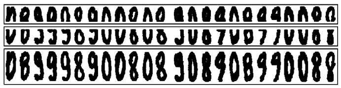
Figure 1: The first row consists of the predictors $X$ which are the upper halves of the image digits $\{0,8,9\}$; The second row consists of the responses $Y$ which are the bottom halves of the image digits $\{0,8,9\}$; The third row consists of the whole image digits $\{0,8,9\}$.

Dubey & Müller (2019) and Petersen & Müller (2019b) provided some fundamental tools for Fréchet analysis of such random objects. Petersen & Müller (2019a) further proposed a general global and local Fréchet regression paradigm for responses being complex random objects in a metric space with Euclidean predictors. Along their pioneering work in Fréchet analysis, it is then of great interest to consider linear and nonlinear sufficient dimension reduction for response objects in a metric space when the dimension of Euclidean predictors is relatively high.

As an illustration of Fréchet sufficient dimension reduction, we consider two models:

$$(\text{i}).\quad Y= (\sin(\beta_{1}^{T}X+\varepsilon_{1})\sin(\beta_{2}^{T}X+\varepsilon_{2}),\sin(\beta_{1}^{T}X+\varepsilon_{1})\cos(\beta_{2}^{T}X+\varepsilon_{2}),\cos(\beta_{1}^{T}X+\varepsilon_{1})),$$

$$(\text{ii}).\quad Y= (\sin(f_{1}(X)+\varepsilon_{1})^{1/3},\cos(f_{1}(X)+\varepsilon_{1})^{1/3}),$$

where $(\varepsilon_{1},\varepsilon_{2})^{T}\sim N(0_{2},I_{2})$, $X=(x_{1},\ldots,x_{p})^{T}\sim N(0_{p},I_{p})$ with $p=30$, $f_{1}(X)=x_{1}^{2}+x_{2}^{2}$, $\beta_{1}=(0.5,0.5,0,\ldots,0)^{T}$, and $\beta_{2}=(0,\ldots,0,0.5,0.5)^{T}$. For models (i) and (ii), the responses lie on unit spheres. Linear Fréchet sufficient dimension reduction for model (i) aims at finding the central subspace $\mathcal{S}_{Y|X}$ with $d=2$, which is the column space spanned by $(\beta_{1},\beta_{2})$. And the purpose of nonlinear Fréchet sufficient dimension reduction for model (ii) is to identify the central class $\mathcal{G}_{Y|X}$ with $d=1$, which is comprised of all measurable functions of $f_{1}(X)$.

To address this issue, we in this paper propose a novel linear Fréchet sufficient dimension reduction method to recover the central subspace $\mathcal{S}_{Y|X}$ defined based on (1) with metric space valued response $Y$. We also provide a consistent estimator of the structural dimension $d$, which is the dimension of the central subspace. The new method is further generalized to nonlinear Fréchet sufficient dimension reduction (2) via the reproducing kernel Hilbert space. The proposed linear and nonlinear Fréchet sufficient dimension reduction estimators are shown to be unbiased for the central subspace $\mathcal{S}_{Y|X}$ and the central class $\mathcal{G}_{Y|X}$ respectively. Moreover, by taking advantage of the distance metric of the random objects, both estimators require no numerical optimization or nonparametric smoothing because they can be easily implemented by spectral decomposition of linear operators. The asymptotic convergence results of our proposal are derived for theoretical justifications. We also examine our method via comprehensive simulation studies including responses that consist of probability distributions or lie on the sphere. And the application to the handwritten digits data demonstrates the practical value of our proposal.

2 Linear Fréchet Sufficient Dimension Reduction

2.1 Weighted Inverse Regression Ensemble

Let $(\Omega,d)$ be a metric space. The linear Fréchet sufficient dimension consider the regression with response variable $Y\in\Omega$ and predictors $X\in\mathbb{R}^{p}$. Let $F$ be the joint distribution of $(X,Y)$ defined on $\mathbb{R}^{p}\times\Omega$. And we assume that the conditional distributions $F_{Y|X}$ and $F_{X|Y}$ exist.

With the linearity condition that $E(X\mid\beta^{T}X)$ is linear in $X$, Li (1991) discovered the fundamental property of sliced inverse regression

$$\Sigma^{-1}\{E(X\mid Y)-E(X)\}\in\mathcal{S}_{Y\mid X},$$ (3)

where $\Sigma=\mbox{var}(X)$. However, the inverse regression mean $E(X|Y)$ is difficult for us to estimate, as only distances between response objects can be computable for responses in metric space.

Our goal for linear Fréchet sufficient dimension is then to borrow the strength of sliced inverse regression without the estimation of the inverse regression function $E(X|Y)$. To introduce our new method, we first recall the martingale difference divergence (MDD) proposed by Shao & Zhang (2014) for $Y\in\mathbb{R}^{q}$ and $X\in\mathbb{R}^{p}$, which is developed to measure the conditional mean (in)dependence of $Y$ on $X$, i.e.

$$E(Y|X)=E(Y),\quad\mbox{almost surely}.$$

To be specific, $\text{MDD}(Y|X)$ is defined as a nonnegative number that satisfies

$$\text{MDD}^{2}(Y|X)=-E\left[\{Y-E(Y)\}^{T}\{Y^{\prime}-E(Y^{\prime})\}\|X-X^{\prime}\|\right],$$

where $(X^{\prime},Y^{\prime})$ is an independent copy of $(X,Y)$, and $\|\cdot\|$ stands for the Euclidean distance.

To inherit the spirit of sliced inverse regression, we switch the roles of $X$ and $Y$ in martingale difference divergence, and define the following $p\times p$ matrix

$$\Lambda=-E\left[\{X-E(X)\}\{X^{\prime}-E(X^{\prime})\}^{T}d(Y,Y^{\prime})\right],$$

for $(X,Y)\in\mathbb{R}^{p}\times\Omega$. By the property of conditional expectation, we have

$$\Lambda=-E\left[E\{X-E(X)|Y\}E\{X^{\prime}-E(X^{\prime})|Y^{\prime}\}^{T}d(Y,Y^{\prime})\right].$$ (4)

Invoking the appealing property (3) of sliced inverse regression, we see that

$$\Sigma^{-1}\Lambda=-\Sigma^{-1}E\left[E\{X-E(X)|Y\}E\{X^{\prime}-E(X^{\prime})|Y^{\prime}\}^{T}d(Y,Y^{\prime})\right]\in\mathcal{S}_{Y|X}.$$

We summarize this property in the following proposition.

Proposition 1.

$\Lambda$ is positive semidefinite. Assume the linearity condition holds true, then

$$\textup{Span}\left\{\Sigma^{-1}\Lambda\right\}\subseteq\mathcal{S}_{Y|X}.$$

From (4), $\Lambda$ can be viewed as the weighted average ensemble of the inverse regression mean $E(X|Y)$, where the weight function is the distance $d(Y,Y^{\prime})$. We thus call our new method as weighted inverse regression ensemble. The weighted inverse regression ensemble can also be applied for classical linear sufficient dimension reduction with $Y\in\mathbb{R}^{q}$ and $d(Y,Y^{\prime})=\|Y-Y^{\prime}\|$ being the Euclidean distance. Moreover, choosing the number of slices for sliced inverse regression is a longstanding issue in the literature. Compared to sliced inverse regression, our proposal is completely slicing free and is readily applicable to multivariate response data.

Let $M=\Sigma^{-1}\Lambda$ and $(\beta_{1},\ldots,\beta_{d})$ be the left singular vectors of $M$ corresponding to the $d$ largest singular values. Then Proposition 6 suggests that $(\beta_{1},\ldots,\beta_{d})$ provides a basis of $\mathcal{S}_{Y\mid X}$. Given a random sample $\{(X_{i},Y_{i}),i=1,\ldots,n\}$ from $(X,Y)$, then $\mu=E(X)$ and $\Sigma=var(X)$ can be estimated as $\hat{\mu}=E_{n}(X)$ and $\hat{\Sigma}=E_{n}\{(X-\hat{\mu})(X-\hat{\mu})^{T}\}$, where $E_{n}(\cdot)$ indicates the sample average $n^{-1}\sum_{i=1}^{n}(\cdot)$. Moreover, we can adopt U-statistics to estimate $\Lambda$ as

$$\hat{\Lambda}=-\sum_{1\leq i\neq j\leq n}(X_{i}-\hat{\mu})(X_{j}-\hat{\mu})^{T}d(Y_{i},Y_{j})/\{n(n-1)\}.$$

Conduct singular value decomposition on $\hat{M}=\hat{\Sigma}^{-1}\hat{\Lambda}$. We then adopt the top $d$ left singular vectors $(\hat{\beta_{1}},\ldots,\hat{\beta}_{d})$ of $\hat{M}$ to recover $\mathcal{S}_{Y|X}$ in the sample level. And we introduce the following notations to present the central limit theory for the estimation of the central subspace.

$$\Gamma(X)=(X-\mu)(X-\mu)^{T}-\Sigma,\quad\Lambda^{(1)}(X,Y,X^{\prime},Y^{\prime})=-(X-\mu)(X^{\prime}-\mu)^{T}d(Y,Y^{\prime}),$$

$$\Lambda^{(1)}_{1}(X^{\prime},Y^{\prime})=E\{\Lambda^{(1)}(X,Y,X^{\prime},Y^{\prime})|X^{\prime},Y^{\prime}\},\quad\vartheta=E\{(X-\mu)d(Y,Y^{\prime})\},$$

$$\Theta(X,Y)=\Lambda^{(1)}_{1}(X,Y)-\Lambda+(X-\mu)\vartheta^{T}+\vartheta(X-\mu)^{T},$$

$$\zeta_{\ell}(X,Y)=\Sigma^{-1}\Big{\{}\Theta(X,Y)\Lambda+\Lambda\Theta(X,Y)-\Gamma(X)\Sigma^{-1}\Lambda\Lambda^{T}-\Lambda\Lambda^{T}\Sigma^{-1}\Gamma(X)\Big{\}}\Sigma^{-1},$$

$$\Upsilon_{\ell}(X,Y)=\sum_{j=1,j\neq\ell}^{p}\frac{\beta_{j}\beta_{j}^{T}\zeta_{\ell}(X,Y)\beta_{\ell}}{\lambda_{j}^{2}-\lambda_{\ell}^{2}},\quad\ell=1,\ldots,d.$$

Theorem 1.

Assume the linearity condition and the singular values $\lambda_{\ell}$’s are distinct for $\ell=1,\ldots,d$. In addition, assume that $Ed^{2}(Y,Y^{\prime})<\infty$ and $X$ has finite fourth moment, then

$$n^{1/2}(\hat{\beta}_{\ell}-\beta_{\ell})\overset{D}{\longrightarrow}N\left({0}_{p},\Sigma_{\ell}\right),$$ (5)

as $n\rightarrow\infty$, where $\Sigma_{\ell}=cov\{\Upsilon_{\ell}(X,Y)\}$.

2.2 Determination of Structural Dimension $d$

The estimation of structural dimension $d$ is another focus in sufficient dimension reduction. We adopt the ladle estimator proposed by Luo & Li (2016) for order determination, which extracts the information contained in both the singular values and the left singular vectors of $M$.

Let $\mathcal{B}_{k}=(\hat{\beta}_{1},\ldots,\hat{\beta}_{k})$ be the $p\times k$ matrix consisting of the principal $d$ left singular vectors of $\hat{M}$. We randomly draw $n$ bootstrap samples of size $n$ and denote the realization of $\mathcal{B}_{k}$ based on the $i$th bootstrap sample as $\mathcal{B}^{*}_{k,i}$. The following function is proposed to evaluate the difference between $\mathcal{B}_{k}$ and its bootstrap counterpart

$$f^{0}_{n}(k)=\begin{cases}0,&k=0,\\ n^{-1}\sum_{i=1}^{n}\{1-|\text{det}(\mathcal{B}_{k}^{T}\mathcal{B}^{*}_{k,i})|\},&k=1,\ldots,p.\end{cases}$$

And $f^{0}_{n}(k)$ is further normalized as $f_{n}(k)=f^{0}_{n}(k)/\{1+\sum_{i=0}^{r_{p}}f_{n}^{0}(i)\},$ where $r_{p}=p-1$ if $p\leq 10$, $r_{p}=\lfloor p/\log p\rfloor$ if $p>10$ and $\lfloor a\rfloor$ stands for the largest integer no greater than $a$. The effect of the singular values are measured as $g_{n}(k)=\hat{\lambda}^{2}_{k+1}/(1+\sum_{{i=0}}^{r_{p}}\hat{\lambda}^{2}_{i+1}),\quad k=0,1,\ldots,r_{p}.$ And the ladle estimator for structural dimension $d$ is constructed as

$$\hat{d}=argmin_{k=0,\ldots,r_{p}}\{f_{n}(k)+g_{n}(k)\}.$$

To obtain the desired estimation consistency of the structural dimension, we assume that

Assumption 1.

The bootstrap version kernel matrix $M^{*}$ satisfies

$$n^{1/2}\{{\mathrm{vech}}(M^{*}(M^{*})^{T})-{\mathrm{vech}}(\widehat{M}(\widehat{M})^{T})\}\rightarrow N(0,{\mathrm{var}}[{\mathrm{vech}}\{H(X,Y)\}])$$ (6)

where ${\mathrm{vech}}(\cdot)$ is the vectorization of the upper triangular part of a matrix and $H(X,Y)=-\Sigma^{-1}(\Gamma(X)-\Sigma)\Sigma^{-1}+\Sigma^{-1}(\Lambda^{(1)}(X,Y)-\Lambda)-\Sigma^{-1}(X-\mu)\vartheta^{T}-\Sigma^{-1}\vartheta(X-\mu)^{T}$.

Assumption 2.

For any sequence of nonnegative random variables $\{Z_{n}:n=1,2,\ldots\}$ involved in this paper, if $Z_{n}=O_{p}(c_{n})$ for some sequence $\{c_{n}:n\in N\}$ with $c_{n}>0$, then $E(c_{n}^{-1}Z_{n})$ exist for each $n$ and $E(c_{n}^{-1}Z_{n})=O(1)$.

From the proof of Theorem 1, we know that $n^{1/2}\{{\mathrm{vech}}(\hat{M}\hat{M}^{T})-{\mathrm{vech}}(MM^{T})\}$ also converges in distribution to the right-hand side of (6). Assumption 1 amounts to asserting that asymptotic behaviour of $n^{1/2}(M^{*}(M^{*})^{T}-\hat{M}\hat{M}^{T})$ mimics that of $n^{1/2}(\hat{M}\hat{M}^{T}-MM^{T})$. The validity of this self-similarity was discussed in Bickel & Freedman (1981), Luo & Li (2016). Assumption 2 has also been adopted and verified by Luo & Li (2016). The following theorem confirms that the number of useful sufficient predictors for linear Fréchet sufficient dimension reduction can be consistently estimated.

Theorem 2.

Assume $Ed^{2}(Y,Y^{\prime})<\infty$ and $X$ has finite fourth moment. And suppose Assumptions (1)–(2) hold, then

$$P_{r}\{\lim_{n\rightarrow\infty}P_{r}(\hat{d}=d|\mathcal{D}){=1}\}=1,$$

where $\mathcal{D}=\{(X_{1},Y_{1}),(X_{2},Y_{2}),\ldots\}$ is a sequence of independent copies of $(X,Y)$.

3 Nonlinear Fréchet Sufficient Dimension Reduction

As the descendant of sliced inverse regression, the weighted inverse regression ensemble method will share the similar limitation with sliced inverse regression when dealing with regression functions that are symmetric about the origin (Cook & Weisberg (1991)). To remedy this problem and to further extend the scope of our method, we in the next will consider nonlinear Fréchet sufficient dimension reduction defined in (2) using the reproducing kernel Hilbert space. Let $\mathcal{H}_{X}$ be a reproducing kernel Hilbert space of functions of $X$ generated by a positive definite kernel $\kappa_{X}$. To extend the idea of weighted inverse regression ensemble for nonlinear Fréceht sufficient dimension reduction, we introduce a new type of operator in the following.

Definition 1.

Let $\mu_{X}(\cdot)=E\kappa_{X}(\cdot,X)$. For $(X,Y)$ and its independent copy $(X^{\prime},Y^{\prime})$, we define the weighted inverse regression ensemble operator $\Lambda_{XX^{\prime}}:\mathcal{H}_{X^{\prime}}\rightarrow\mathcal{H}_{X}$ such that

$$\Lambda_{XX^{\prime}}=-E\{(\kappa_{X}(\cdot,X)-\mu_{X}(\cdot))\otimes(\kappa_{X}(\cdot,X^{\prime})-\mu_{X^{\prime}}(\cdot))d(Y,Y^{\prime})\}.$$

We assume the following regularity assumptions for theoretical investigations into $\Lambda_{XX^{\prime}}$.

Assumption 3.

$E\kappa_{X}(X,X)<\infty$.

Assumption 4.

The operator $\Lambda_{XX^{\prime}}$ has a representation as $\Lambda_{XX^{\prime}}=\Sigma_{XX}S$, where $S$ is a unique bounded linear operator such that $S:\mathcal{H}_{X}\rightarrow\mathcal{H}_{X}$, $S=Q_{X}SQ_{X}$ with $Q_{X}$ being the projection operator mapping $\mathcal{H}_{X}$ on to $\overline{\mathrm{ran}}(\Sigma_{XX})$, and $\overline{\mathrm{ran}}(\Sigma_{XX})$ stands for the closure of the range of the covariance operator $\Sigma_{XX}$.

Assumption 5.

$\mathcal{G}_{Y|X}$ is dense in $L_{2}(P_{X}|\mathcal{M}_{Y|X})$, where $L_{2}(P_{X}|\mathcal{M}_{Y|X})$ denotes the collection of $\mathcal{M}_{Y|X}$-measurable functions in $L_{2}(P_{X})$ and $\mathcal{M}_{Y|X}=\sigma[f(X)]$.

Assumption 6.

The eigenfunctions $\psi_{i}$’s are included in $\mathcal{R}(\Sigma_{XX})$, where $\mathcal{R}(\Sigma_{XX})=\{\Sigma_{XX}f:f\in\mathcal{H}_{X}\}$.

Assumption 7.

Let $(\varepsilon_{n})_{n=1}^{\infty}$ be a sequence of positive numbers such that

$$\lim_{n\rightarrow\infty}\varepsilon_{n}=0,\ \ \ \lim_{n\rightarrow\infty}n^{-1/2}/\varepsilon_{n}^{3/2}=0.$$

.

Assumption 3, 5 and 6 are commonly used conditions for reproduce kernel Hilbert spaces in the literature (Lee et al. (2013); Li (2018)). Assumption 4 is similar to the result of Theorem 1 of Baker (1973) that defines the correlation operator, which will guarantee that our proposed operator is compact. Assumption 7 is adopted by Fukumizu et al. (2007) for asymptotic analysis of kernel type methods, which is helpful to establish the estimation consistency of nonlinear weighted inverse regression ensemble method.

Proposition 2.

$\Lambda_{XX^{\prime}}$ is a bounded linear and self-adjoint operator. For any $f,g\in\mathcal{H}_{X}$,

$$\langle f,\Lambda_{XX^{\prime}}g\rangle=-E\{(f(X)-Ef(X))(g(X^{\prime})-E{g(X^{\prime})})d(Y,Y^{\prime})\}.$$

Moreover, there exists a separable $\mathbb{R}$-Hilbert space $\mathcal{H}$ and a mapping $\phi:\Omega\rightarrow\mathcal{H}$ such that

$$\langle f,\Lambda_{XX^{\prime}}f\rangle=2\{E[(f(X)-Ef(X))(\phi(Y)-E\phi(Y))]\}^{2}=2(cov[f(X),\phi(Y)])^{2}.$$

Proposition 2 implies that our proposed new operator enjoys a similar fashion as the commonly used covariance operator. The new operator also has the potential to measure the dependence between Euclidean $X$ and random objects $Y$ due to its similarity to the popular Hilbert-Schmidt Independence Criterion (Gretton et al. (2005)). Denote the covariance operator of $X$ as $\Sigma_{XX}=E\{\kappa_{X}(\cdot,X)\otimes\kappa_{X}(\cdot,X)\}-E\kappa_{X}(\cdot,X)\otimes E\kappa_{X}(\cdot,X)$.. The next proposition reveals the relationship between $\Lambda_{XX^{\prime}}$ and the central class $\mathcal{G}_{Y|X}$.

Proposition 3.

Suppose assumptions (3)–(5) hold, then

$$\overline{\textup{ran}}\left\{\Sigma_{XX}^{-1}\Lambda_{XX^{\prime}}\right\}\subseteq\mathcal{G}_{Y|X}.$$

Proposition 4.

Suppose assumptions (3)–(5) hold and $\mathcal{G}_{Y|X}$ is complete. Then,

$$\overline{\textup{ran}}\left\{\Sigma_{XX}^{-1}\Lambda_{XX^{\prime}}\right\}=\mathcal{G}_{Y|X}.$$

Proposition 8 suggests that the range of $\Sigma_{XX}^{-1}\Lambda_{XX^{\prime}}$ is always contained in the central class $\mathcal{G}_{Y|X}$. Proposition 9 further extends the scope in the following aspects. First, it confirms that the nonlinear weighted inverse regression ensemble method is exhaustive in recovering the central class. The exhaustiveness of our nonlinear proposal is an appealing property which may not exist in the linear setting. The second is that the nonlinear weighted inverse regression ensemble method leads to the minimal sufficient predictor satisfying (2), as sufficiency and completeness together imply minimal sufficiency in classical statistical inference. Last but not least, the nonlinear weighted inverse regression ensemble method does not rely on the linear conditional mean assumption requiring that $E(X|\beta^{T}X)$ be linear in $X$. By relaxing such a stringent condition, the nonlinear method will have a wide range of applications.

Let $\Lambda_{XX^{\prime}}^{*}$ be the adjoint operator of $\Lambda_{XX^{\prime}}$. Proposition 9 indicates that

$$\overline{\textup{ran}}\left\{\Sigma_{XX}^{-1}\Lambda_{XX^{\prime}}\Lambda_{XX^{\prime}}^{*}\Sigma_{XX}^{-1}\right\}=\mathcal{G}_{Y|X},$$ (7)

The space (7) can be recovered by performing the following generalized eigenvalue problem:

$$\mathrm{max}\ \ \langle f,\Lambda_{XX^{\prime}}\Lambda_{XX^{\prime}}^{*}f\rangle_{\mathcal{H}_{X}},\ \mathrm{s.t.}\ \langle f,\Sigma_{XX}f\rangle_{\mathcal{H}_{X}}=1,f\bot\mathcal{L}_{k-1},$$ (8)

where $\mathcal{L}_{k}=\textup{Span}(f_{1},\ldots,f_{k-1})$ and $f_{1},\ldots,f_{k-1}$ are the solutions to this constrained maximization problem in the previous steps. Define the following sample level estimators

$$\hat{\mu}_{X}(\cdot)=E_{n}[\kappa_{X}(\cdot,X_{i})]\quad\hat{\Sigma}_{XX}=E_{n}\{(\kappa_{X}(\cdot,X_{i})-\hat{\mu}_{X}(\cdot))\otimes(\kappa_{X}(\cdot,X_{i})-\hat{\mu}_{X}(\cdot))\},$$

$$\hat{\Lambda}_{XX}=-\sum_{1\leq i\neq j\leq n}(\kappa_{X}(\cdot,X_{i})-\hat{\mu}_{X}(\cdot))\otimes(\kappa_{X}(\cdot,X_{j})-\hat{\mu}_{X}(\cdot))d(Y_{i},Y_{j})/(n(n-1)).$$

The sample version of (8) then becomes

$$\mathrm{max}\ \ \langle f,\widehat{\Lambda}_{XX^{\prime}}\widehat{\Lambda}_{XX^{\prime}}^{*}f\rangle_{\mathcal{H}_{X}},\ \mathrm{s.t.}\ \langle f,(\widehat{\Sigma}_{XX}+\varepsilon_{n}I)f\rangle_{\mathcal{H}_{X}}=1.$$ (9)

Let $V_{XX^{\prime}}=\Sigma_{XX}^{-1/2}\Lambda_{XX^{\prime}}\Lambda_{XX^{\prime}}^{*}\Sigma_{XX}^{-1/2}$. Then we can verify that $f_{1}=\Sigma_{XX}^{-1/2}\psi_{1}$, where

$$\psi_{1}=\arg\max_{\begin{subarray}{c}g\in\mathcal{H}_{X},\|g\|_{\mathcal{H}_{X}}=1\end{subarray}}\langle g,V_{XX^{\prime}}g\rangle_{\mathcal{H}_{X}}.$$

Let $\hat{V}_{XX^{\prime}}=(\hat{\Sigma}_{XX}+\varepsilon_{n}I)^{-1/2}\hat{\Lambda}_{XX^{\prime}}\hat{\Lambda}_{XX^{\prime}}^{*}(\hat{\Sigma}_{XX}+\varepsilon_{n}I)^{-1/2}$. Then we have

$$\hat{f}_{1}(X)=(\hat{\Sigma}_{XX}+\varepsilon_{n}I)^{-1/2}\hat{\psi}_{1},\quad\hat{\psi}_{1}=\arg\max_{\begin{subarray}{c}g\in\mathcal{H}_{X},\|g\|_{\mathcal{H}_{X}}=1\end{subarray}}\langle g,\hat{V}_{XX^{\prime}}g\rangle_{\mathcal{H}_{X}}.$$

We in the next establish the estimation consistency of our nonlinear Frécechet sufficient dimension reduction approach. Although we only focus on the first eigenfunction in the following theorem, similar asymptotic results can be derived for the entire central .

Theorem 3.

Suppose assumptions (3)–(7) hold. In addition, assume that $Ed^{2}(Y,Y^{\prime})<\infty$, then as $n\rightarrow\infty$

$$\|\hat{V}_{XX^{\prime}}-V_{XX^{\prime}}\|_{\text{HS}}=o_{p}(1),\ \ \ |\langle\hat{\psi}_{1},\psi_{1}\rangle_{\mathcal{H}_{X}}|\stackrel{{\scriptstyle P}}{{\longrightarrow}}1,$$

$$\|\{\hat{f}_{1}(X)-E\hat{f}_{1}(X)\}-\{f_{1}(X)-Ef_{1}(X)\}\|{\longrightarrow}0,$$

where $\|\cdot\|$ in this theorem is the standard $L_{2}$ norm to measure the distance of functions and $\|\cdot\|_{\text{HS}}$ denotes the Hilbert-Schmidt norm.

Let $\eta_{i}={{\kappa_{X}(\cdot,X_{i})}}-\hat{\mu}_{X}(\cdot),i=1,\ldots,n$. The estimated eigenfunctions $\hat{f}_{\ell}$’s solved from (9) can be further characterized as a linear combination of $\eta_{i}$ such that $\hat{f}_{\ell}=\sum_{i=1}^{n}a_{\ell,i}\eta_{i}$. Denote $\alpha_{\ell}=(a_{\ell,1},\ldots,a_{\ell,n})^{T}$. The next proposition indicates that $\alpha_{\ell}$ can be obtained through solving an eigen-decomposition problem.

Proposition 5.

Let $K_{n}$ be the $n\times n$ kernel matrix whose $(i,j)$th element is $\kappa_{X}(X_{i},X_{j})$. Denote $J_{n}$ as the $n\times n$ matrix whose elements are all one. Define $G_{X}=(I_{n}-J_{n}/n)K_{n}(I_{n}-J_{n}/n)$ and let $D_{Y}$ be the $n\times n$ matrix whose $(i,j)$th element is $d(Y_{i},Y_{j})$. Then we have $G_{X}\alpha_{\ell}=\gamma_{\ell}$, where $\gamma_{\ell}$ is the $\ell$th eigenvector of the following matrix

$$(G_{X}+\varepsilon_{n}I_{n})^{-1}G_{X}D_{Y}G_{X}D_{Y}G_{X}(G_{X}+\varepsilon_{n}I_{n})^{-1}.$$

Let $\hat{\alpha}_{\ell}=(G_{X}+\varepsilon_{n}I_{n})^{-1}\gamma_{\ell}$. Inspired by Proposition 4, the $\ell$th estimated sufficient predictor can then be represented as $\hat{f}_{\ell}=\sum_{i=1}^{n}\hat{a}_{\ell,i}\eta_{i}$, where $\hat{a}_{\ell,i}$ is the $i$th element of the $n\times 1$ vector $\hat{\alpha}_{\ell}$.

4 Numerical Studies

We consider the following models with responses being complex random objects.

Model I. Let $\beta_{1}=(1,1,0,\ldots,0)^{T}$ and $\beta_{2}=(0,\ldots,0,1,1)^{T}$. $X\sim U[0,1]^{p}$ and $Y$ is the distribution function with its quantile function being $Q_{Y}(\tau)=\mu_{Y}+\sigma_{Y}\Phi^{-1}(\tau)$, where $\Phi(\cdot)$ is the cumulative distribution function of standard normal, $\mu_{Y}|X\sim N(\exp(\beta_{1}^{T}X),0.5^{2})$. And we consider $\sigma_{Y}=1$ as case (i) and $\sigma_{Y}=|\beta_{2}^{T}X|$ as case (ii). As $Y$ and its independent copy $Y^{\prime}$ are random distribution functions, then we adopt the Wasserstein distance as the metric $d(Y,Y^{\prime})$. For case (i), $\mathcal{S}_{Y|X}=\text{Span}(\beta_{1})$ and $d=1$. For case (ii), $\mathcal{S}_{Y|X}=\text{Span}(\beta_{1},\beta_{2})$ and $d=2$.

Model II. Consider the following Fréchet regression function

$${m(X)=(\cos(f_{1}(X)),\sin(f_{1}(X)))}.$$

Generate $\varepsilon$ from $N(0,0.1^{2})$ on the tangent line of $m(x)$. And the response $Y$ is generated as

$$Y=\cos(\varepsilon)m(x)\oplus\sin(\varepsilon)\varepsilon/|\varepsilon|,$$

where $\oplus$ stands for vector addition. We can verify that $Y\in\Omega$ where $\Omega$ is the unit circle in $\mathbb{R}^{2}$. Then $d(Y,Y^{\prime})$ is naturally chosen as the geodesic distance $\arccos(Y^{T}Y^{\prime})$. Moreover, we consider case (i) $f_{1}(X)=\beta_{1}^{T}X$ with $X\sim U[0,1]^{p}$ and cased (ii) where $f_{1}(X)=(x_{1}^{2}+x_{2}^{2})^{1/2}$ with $X\sim N(0_{p},I_{p})$ for both linear and nonlinear Fréchet sufficient dimension reduction.

Model III. Generate $\varepsilon_{i}$ from $N(0,0.1^{2})$ for $i=1,2$. We consider two cases in this study. The model structure of case (i) is exactly the same as our motivating example (i) illustrated in Section 1 with $X\sim U[0,1]^{p}$. For case (ii), the response $Y$ is generated as

$$Y=(\sin(f_{1}(X)+\varepsilon_{1})^{1/3}\sin(f_{2}(X)+\varepsilon_{2})^{1/3},\sin(f_{1}(X)+\varepsilon_{1})^{1/3}\cos(f_{2}(X)+\varepsilon_{2})^{1/3},\cos(f_{1}(X)+\varepsilon_{1})^{1/3}),$$

where $f_{1}(X)=x_{1}^{2}+x_{2}^{2}$ and $f_{2}(X)=x^{2}_{p-1}+x^{2}_{p}$, and $X\sim N(0_{p},I_{p})$. We see that $Y\in\Omega$ where $\Omega$ is the unit sphere in $\mathbb{R}^{3}$. Again $d(Y,Y^{\prime})=\arccos(Y^{T}Y^{\prime})$ is the geodesic distance.

Model I and case (i) of and Model II and III are adopted for linear Fréchet sufficient dimension reduction, while the two rest cases are examples for nonlinear Fréchet sufficient dimension reduction. Let $\hat{\beta}$ and $\hat{f}(X)$ be our proposed linear and nonlinear weighted inverse regression estimators. To evaluate our proposal for linear Fréchet sufficient dimension reduction, we adopt the trace correlation (Ferré (1998)) defined as $r^{2}=tr(P_{\beta}P_{\hat{\beta}})/d$ , where $P_{\beta}=\beta(\beta^{T}\beta)^{-1}\beta^{T}$. To assess the performance of nonlinear Fréchet sufficient dimension reduction, we utilize the square distance correlation $\rho^{2}(f(X),\hat{f}(X))$ proposed by Székely et al. (2007). The square distance correlation can also be adapted to linear Fréchet sufficient dimension reduction as $\rho^{2}(\beta^{T}X,\hat{\beta}^{T}X)$. And larger values of $r^{2}$ or $\rho^{2}$ indicate better estimation.

We consider $n=100,200,300,400$ and $p=10,20,30$. Treating $d$ as known, Table 1 and 2 summarize the mean values of $r^{2}$ and $\rho^{2}$ based on 100 repetitions with different combinations of $n$ and $p$. We can see from Table 1 that the original weighted inverse regression ensemble works well except for case (ii) of Model II and III with U-shape structure, which is consistent with our theoretical anticipation. As an effective remedy, the nonlinear weighted inverse regression produces a satisfying result as seen from Table 2, in which the tuning parameter is simply set as $\varepsilon_{n}=0.001$ and Gaussian kernel $\kappa_{X}(X,X^{\prime})=\exp\{-\|X-X^{\prime}\|^{2}/(2\sigma^{2}_{\kappa})\}$ is adopted with $\sigma_{\kappa}=0.1$. The results for order determination are presented in Table 3, where the entries are the number of correct estimation of $d$ out of $100$ repetitions. Table 3 shows that the ladle estimator in combination with weighted inverse regression ensemble works well, with percentage of correct estimation reaching as high as $100\%$ for most cases.

Table 1: The Averages of $r^{2}$ and $\rho^{2}$ for the estimation of $\mathcal{S}_{Y|X}$ based on $100$ simulation runs.

		Model I				Model II				Model III
	$(p,n)$	100	200	300	400	100	200	300	400	100	200	300	400
Case i	10	0.979	0.988	0.993	0.995	0.988	0.996	0.997	0.998	0.987	0.995	0.996	0.997
		0.973	0.984	0.990	0.993	0.988	0.994	0.996	0.967	0.987	0.994	0.995	0.997
	20	0.947	0.976	0.976	0.989	0.971	0.991	0.994	0.995	0.966	0.986	0.991	0.994
		0.943	0.970	0.970	0.985	0.970	0.989	0.992	0.993	0.873	0.986	0.990	0.993
	30	0.908	0.960	0.976	0.982	0.961	0.987	0.990	0.992	0.945	0.977	0.986	0.989
		0.917	0.955	0.970	0.976	0.964	0.985	0.988	0.990	0.959	0.978	0.985	0.989
Case ii	10	0.990	0.995	0.997	0.998	0.255	0.253	0.234	0.278	0.379	0.369	0.382	0.377
		0.989	0.994	0.996	0.997	0.122	0.092	0.078	0.085	0.231	0.178	0.166	0.156
	20	0.976	0.988	0.993	0.995	0.136	0.125	0.123	0.134	0.177	0.188	0.188	0.196
		0.978	0.989	0.992	0.994	0.092	0.053	0.038	0.039	0.163	0.097	0.078	0.068
	30	0.956	0.982	0.988	0.991	0.094	0.085	0.084	0.094	0.118	0.122	0.126	0.134
		0.967	0.982	0.987	0.991	0.085	0.048	0.032	0.028	0.147	0.081	0.060	0.049

Table 2: *

The average $r^{2}$ and $\rho^{2}$ are listed in the first and second rows for each $p$.

Table 3: The Averages of $\rho^{2}$ for the estimation of $\mathcal{G}_{Y|X}$ based on $100$ simulation runs.

	Model II (case ii)					Model III (case ii)
$(p,n)$	100	200	300	400	$(p,n)$	100	200	300	400
10	0.948	0.952	0.952	0.952	10	0.818	0.828	0.827	0.828
20	0.952	0.952	0.951	0.952	20	0.823	0.834	0.828	0.829
30	0.952	0.951	0.952	0.952	30	0.827	0.826	0.827	0.827

Table 4: The number of correctly estimation for $d$ among $100$ simulation runs.

	Model I (case i)				Model I (case ii)				Model II (case i)				Model III (case i)
$(p,n)$	100	200	300	400	100	200	300	400	100	200	300	400	100	200	300	400
10	100	100	100	100	100	100	100	100	100	100	100	100	100	100	100	100
20	100	100	100	100	100	100	100	100	100	100	100	100	100	100	100	100
30	100	100	100	100	100	100	100	100	100	100	100	100	99	100	100	100

To better illustrate the performance of our nonlinear Fréchet sufficient dimension reduction method, we in Figure 2 present the 2-D scatter plots for the nonlinear sufficient predictors from case (ii) of Model III versus their sample estimates obtained by the nonlinear weighted inverse regression ensemble method with $n=100$ and $p=10$. The left panel is the 2-D scatter plots for the first nonlinear sufficient predictor $f_{1}(X)=x_{1}^{2}+x_{2}^{2}$ versus its estimate $\hat{f}_{1}(X)$; the right panel is the 2-D scatter plots for the second nonlinear sufficient predictor $f_{2}(X)=x_{p-1}^{2}+x_{p}^{2}$ versus its estimate $\hat{f}_{2}(X)$. Figure 2 shows a strong relationship between $f_{i}$ and $\hat{f}_{i}$ for $i=1,2$. $\hat{f}_{i}$ behaves like a measurable function of $f_{i}$, which is consistent with our theoretical development as our focus on nonlinear Fréchet sufficient dimension reduction is the $\sigma$-field generated by $f_{1}$ and $f_{2}$ rather than $f_{1}$ and $f_{2}$ themselves. As $f^{1/3}_{i}$ is a measurable function of $f_{i}$, then $f_{i}^{1/3}$ can also be regarded as the nonlinear sufficient predictor. We in Figure 3 present the 2-D scatter plots for the nonlinear sufficient predictors $f_{1}^{1/3}$ and $f_{2}^{1/3}$ versus $\hat{f}_{1}$ and $\hat{f}_{2}$. We can observe a strong linear pattern between $f^{1/3}_{i}$ and $\hat{f}_{i}$, which again verify that our proposed nonlinear weighted inverse regression ensemble method is effect in recovering the central class $\mathcal{G}_{Y|X}$ with responses $Y$ being metric space valued random objects.

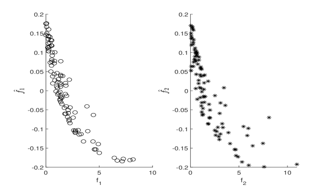
Figure 2: Scatter plots of nonlinear sufficient predictors $f_{i}$’s versus their estimates $\hat{f}_{i}$’s.

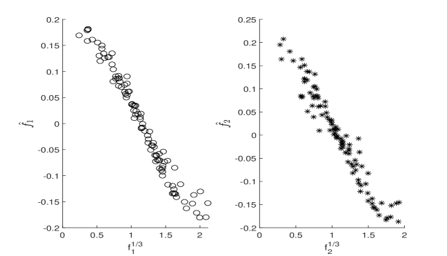
Figure 3: Scatter plots of nonlinear sufficient predictors $f^{1/3}_{i}$’s versus their estimates $\hat{f}_{i}$’s.

5 Handwritten Digits Data

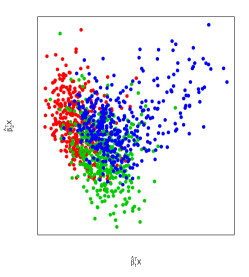
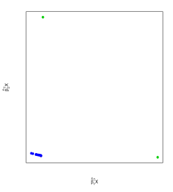
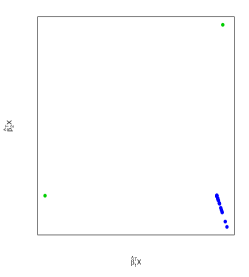
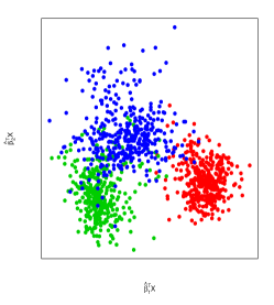
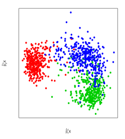
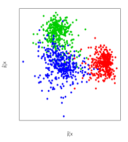
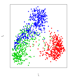
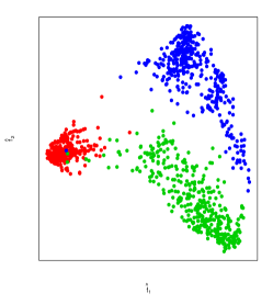
Figure 4: The first row consists of the scatter plots for the training data via projective resampling based Slice Inverse Regression(SIR), Slice Average Variance Estimation(SAVE), Directional Regression(DR), respectively. The second row consists of the scatter plots based on our linear proposal with Euclidean distance, Locally Linear Embedding (LLE) and Isomap, respectively. The third row consists of the scatter plots based on our nonlinear proposal with Euclidean distance, LLE and Isomap, respectively. (red: $0$; green: $8$;blue: $9$.)

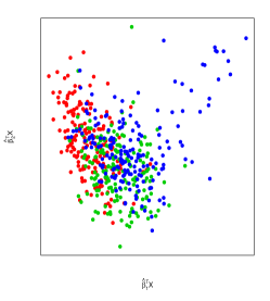
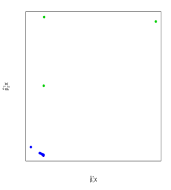
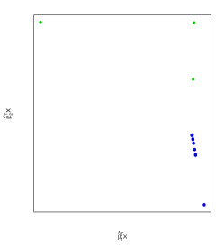
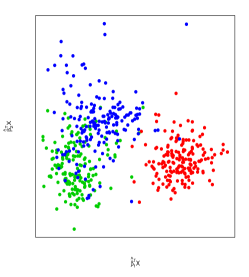
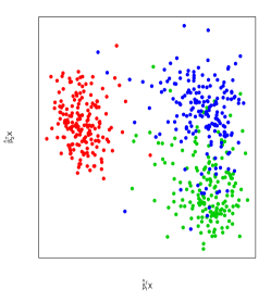
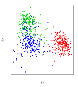
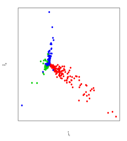
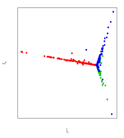
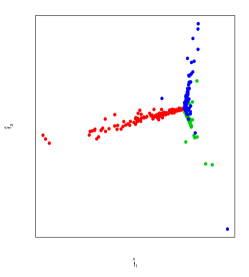
Figure 5: The first row consists of the perspective plots for the first two sufficient predictors for the testing data by projective resampling based SIR, SAVE and DR, respectively. The second row consists of the perspective plots for the testing data based on our linear proposal with Euclidean distance, LLE and Isomap, respectively. The third row consists of the perspective plots for our nonlinear proposal with Euclidean distance, LLE and Isomap. (red: $0$; green: $8$;blue: $9$.)

To further investigate the performance of our proposals and demonstrate its use in real applications, we now extract $1670$ gray-scale images of three handwritten digit classes $\{0,8,9\}$, from the UCI Machine Learning Repository. This dataset contains a training group of size $1138$ and a testing group of size $532$. Each digit was represented by an $8\times 8$ pixel image. The $4\times 8$ upper part of each image was taken as the predictors $X$, and the $4\times 8$ bottom half was set as the responses $Y$.

We focus on sufficient dimension reduction of the $32$-dimensional feature vectors $X$ for the training set, which serves as a preparatory step for further clustering or classification. Because the response $Y$ is also $32$-dimensional, we include the projective resampling approach (Li et al. (2008)) for comparisons, as it is the state of the art sufficient dimension reduction paradigm for multivariate response data. To be specific, we consider projective resampling approach in combination with three classical methods; sliced inverse regression, sliced average variance estimation and directional regression. And we adopt three different distance metrics for our proposals: the Euclidean distance, the distance metric learned by the Local Linear Embedding (Roweis & Saul (2000)), the distance metric learned by the Isomap approach (Tenenbaum et al. (2009)).

For the training data, Figure 4 presents the scatter plots of the first two sufficient predictors estimated by projective resampling based three classical methods, as well as our proposed linear and nonlinear weighted inverse regression ensemble methods, with the cases for digits 0, 8 and 9 represented by red, green and blue dots respectively. Figure 4 shows that the linear weighted inverse regression ensemble method performs much better than the classical methods. We also observe that our nonlinear weighted inverse regression ensemble method based on the distance metric induced by the Isomap approach provides better separation both in location and variation, which should be useful for further classification.

Figure 5 presents the perspective plots for the testing data. Similar to our previous findings, our linear and nonlinear weighted inverse regression ensemble approaches again do a much better job in separating the three digit classes compared to the classical methods. The upper parts of digits $8$ and $9$ are generally difficult to distinguish. However, our proposals provide valid and useful information for classification as seen from the scatter plots.

6 Discussion

When the predictor dimension is excessively large, we may consider sparse Fréchet dimension reduction with response as random objects and ultrahigh dimensional predictor. The proposed weighted inverse regression ensemble method can be further extended for model free variable selection and screening (Yin & Hilafu (2015); Yu et al. (2016)) and minimax estimation of $\mathcal{S}_{Y|X}$ (Tan et al. (2019)). The full potential of sparse Fréchet dimension reduction will be further explored in future research.

Supplement to “Fréchet Sufficient Dimension Reduction for Random Objects”

Appendix A Additional Simulation Studies

In addition to models I-III adopted in the main paper, we consider a new model here.

Model IV.

$$Y=(\cos(\varepsilon_{1})\sin(f_{1}(X))\sin(f_{2}(X)),\cos(\varepsilon_{1})\sin(f_{1}(X))\cos(f_{2}(X)),\cos(\varepsilon_{1})\cos(f_{1}(X)),\sin(\varepsilon_{1})).$$

For Model IV, the response is a 4-dimensional vector and the fourth dimension can be viewed as a noise term which does not contain any valid information. Moreover, $Y\in\Omega$ where $\Omega$ is the unit sphere in $\mathbb{R}^{4}$. And the metric equipped with $\Omega$ is the geodesic distance $d(Y,Y^{\prime})=\arccos(Y^{T}Y^{\prime})$. Generate $\varepsilon_{1}$ from $N(0,0.1^{2})$. We consider case (i) where $f_{1}(X)=\beta_{1}^{T}X$ and $f_{2}(X)=\beta_{2}^{T}X$ with $\beta_{1}=(0.5,0.5,0,\ldots,0)^{T}$ and $\beta_{2}=(0,\ldots,0,0.5,0.5)^{T}$ and cased (ii) where $f_{1}(X)=0.5(x_{1}^{2}+x_{2}^{2})^{1/2}$ and $f_{1}(X)=0.5(x_{p-1}^{2}+x_{p}^{2})^{1/2}$ for both linear and nonlinear Fréchet sufficient dimension reduction.

We design the following scenarios for the predictors for models I-IV.

Scenario 1. $X$ is generated from the multivariate normal distribution $N(\alpha,I_{p})$, where $\alpha\sim U[0,1]^{p}$. The results for the four models, including linear Fréchet sufficient dimension reduction, nonlinear Fréchet sufficient dimension reduction and order determination, are presented in Table A.1-A.3.

Scenario 2. $X$ is generated from the multivariate normal distribution $N(\alpha,\Sigma)$, where $\alpha\sim U[0,1]^{p}$ and $\Sigma=\{(\sigma_{ij})_{p\times p}:\sigma_{ij}=0.2^{|i-j|}\}$. The results of the four models under scenario 2 are summarized in Table A.4-A.6.

Scenario 3. $x_{i}$ is generated from the poisson distribution $P_{\lambda}$ with $\lambda=1$ for $i=1,\ldots,p$. $x_{i}$ and $x_{j}$ are independent of each other. The results of the four models under scenario 3 are presented in Table A.7 -A.9.

Scenario 4. $x_{i}$ is generated from the exponential distribution distribution $\text{Exp}(\lambda)$ with $\lambda=1$ for $i=1,\ldots,p$. $x_{i}$ and $x_{j}$ are independent of each other. The results of the four models under scenario 4 are presented in Table A.10-A.12.

We see from these tables our proposal gives quite promising results for Frćhet sufficient dimension reduction and order determination. When the weighted inverse regression ensemble method fail to work with symmetric regression function, its nonlinear extension always make a good remedy. Our proposed methods along with the asymptotic theories are robust to different model settings, except for order determination with case (ii) of Model I under scenario 2.

Table 5: The means of $r^{2}$ and $\rho^{2}$ for estimating $\mathcal{S}_{Y|X}$ among repetitions with scenario 1.

Model I (case i)						Model I (case ii)
$(p,n)$	100	200	300	400	$(p,n)$	100	200	300	400
10	0.912	0.938	0.955	0.967	10	0.869	0.923	0.954	0.961
	0.891	0.917	0.938	0.952		0.872	0.917	0.947	0.955
20	0.790	0.876	0.910	0.927	20	0.771	0.869	0.911	0.919
	0.787	0.851	0.884	0.905		0.798	0.862	0.904	0.909
30	0.707	0.817	0.858	0.888	30	0.688	0.830	0.854	0.894
	0.731	0.799	0.827	0.861		0.752	0.839	0.849	0.884
Model II(case i)						Model II(case ii)
$(p,n)$	100	200	300	400	$(p,n)$	100	200	300	400
10	0.915	0.963	0.974	0.982	10	0.471	0.510	0.529	0.531
	0.915	0.953	0.966	0.974		0.375	0.392	0.421	0.392
20	0.827	0.918	0.946	0.961	20	0.387	0.439	0.451	0.467
	0.866	0.914	0.936	0.951		0.372	0.361	0.338	0.381
30	0.766	0.874	0.912	0.937	30	0.314	0.382	0.413	0.424
	0.850	0.886	0.909	0.929		0.328	0.337	0.339	0.326
Model III (case i)						Model III (case ii)
$(p,n)$	100	200	300	400	$(p,n)$	100	200	300	400
10	0.891	0.946	0.971	0.976	10	0.538	0.577	0.586	0.584
	0.895	0.941	0.966	0.973		0.476	0.508	0.512	0.514
20	0.810	0.898	0.924	0.941	20	0.401	0.464	0.463	0.493
	0.843	0.901	0.919	0.934		0.453	0.466	0.445	0.465
30	0.735	0.856	0.900	0.922	30	0.333	0.391	0.427	0.444
	0.813	0.870	0.902	0.919		0.424	0.426	0.446	0.438
Model IV (case i)						Model IV (case ii)
$(p,n)$	100	200	300	400	$(p,n)$	100	200	300	400
10	0.920	0.949	0.966	0.978	10	0.591	0.607	0.622	0.627
	0.921	0.945	0.962	0.974		0.430	0.433	0.451	0.448
20	0.803	0.877	0.934	0.944	20	0.431	0.484	0.501	0.520
	0.832	0.879	0.930	0.938		0.387	0.379	0.373	0.388
30	0.733	0.840	0.888	0.911	30	0.358	0.419	0.449	0.454
	0.806	0.856	0.890	0.907		0.365	0.356	0.371	0.366

Table 6: *

The average $r^{2}$ and $\rho^{2}$ are listed in the first and second rows for each $p$.

Table 7: The means of $\rho^{2}$ for estimating $\mathcal{G}_{Y|X}$ among $100$ repetitions with scenario 1.

	Model II (case ii)				Model III (case ii)				Model IV (case ii)
$(p,n)$	100	200	300	400	100	200	300	400	100	200	300	400
10	0.986	0.957	0.957	0.957	0.843	0.840	0.839	0.844	0.940	0.940	0.942	0.941
20	0.954	0.958	0.956	0.956	0.843	0.835	0.837	0.839	0.941	0.942	0.942	0.943
30	0.956	0.956	0.955	0.955	0.840	0.838	0.834	0.838	0.940	0.942	0.943	0.941

Table 8: The number of correctly estimation for $d$ among $100$ repetitions with scenario 1.

Model I (case i)					Model I (case ii)					Model II (case i)
$(p,n)$	100	200	300	400	$(p,n)$	100	200	300	400	$(p,n)$	100	200	300	400
10	100	100	100	100	10	41	59	63	70	10	85	96	99	99
20	100	100	100	100	20	22	38	40	53	20	78	96	100	100
30	100	100	100	100	30	18	31	36	43	30	23	70	94	100
Model III (case i)					Model IV (case i)
$(p,n)$	100	200	300	400	$(p,n)$	100	200	300	400
10	38	45	48	60	10	74	90	87	90
20	10	21	29	35	20	49	72	82	83
30	2	16	27	32	30	37	65	70	67

Table 9: The means of $r^{2}$ and $\rho^{2}$ for estimating $\mathcal{S}_{Y|X}$ among $100$ repetitions with scenario 2.

Model I (case i)						Model I (case ii)
$(p,n)$	100	200	300	400	$(p,n)$	100	200	300	400
10	0.854	0.913	0.933	0.947	10	0.840	0.880	0.931	0.937
	0.862	0.909	0.929	0.943		0.872	0.895	0.939	0.945
20	0.720	0.823	0.848	0.881	20	0.711	0.781	0.846	0.881
	0.764	0.830	0.848	0.878		0.791	0.820	0.866	0.896
30	0.617	0.766	0.795	0.837	30	0.584	0.767	0.794	0.836
	0.689	0.783	0.807	0.839		0.716	0.816	0.826	0.856
Model II (case i)						Model II (case ii)
$(p,n)$	100	200	300	400	$(p,n)$	100	200	300	400
10	0.853	0.920	0.948	0.963	10	0.249	0.258	0.247	0.250
	0.888	0.930	0.947	0.962		0.131	0.101	0.084	0.088
20	0.707	0.853	0.900	0.921	20	0.128	0.141	0.121	0.158
	0.814	0.881	0.908	0.925		0.097	0.059	0.042	0.051
30	0.603	0.753	0.842	0.883	30	0.086	0.086	0.085	0.099
	0.778	0.827	0.873	0.897		0.100	0.049	0.032	0.029
Model III(case i)						Model III (case ii)
$(p,n)$	100	200	300	400	$(p,n)$	100	200	300	400
10	0.864	0.916	0.943	0.957	10	0.365	0.383	0.373	0.353
	0.896	0.930	0.950	0.961		0.243	0.192	0.173	0.154
20	0.749	0.830	0.898	0.904	20	0.181	0.189	0.184	0.182
	0.819	0.862	0.915	0.918		0.160	0.106	0.078	0.069
30	0.687	0.794	0.842	0.862	30	0.114	0.123	0.118	0.122
	0.799	0.840	0.873	0.886		0.144	0.086	0.063	0.050
Model IV (case i)						Model IV (case ii)
$(p,n)$	100	200	300	400	$(p,n)$	100	200	300	400
10	0.844	0.915	0.946	0.959	10	0.595	0.613	0.631	0.644
	0.877	0.930	0.953	0.964		0.504	0.478	0.510	0.526
20	0.731	0.843	0.881	0.916	20	0.424	0.472	0.505	0.523
	0.808	0.873	0.901	0.927		0.439	0.435	0.444	0.473
30	0.660	0.803	0.828	0.877	30	0.339	0.412	0.445	0.462
	0.783	0.853	0.864	0.898		0.409	0.415	0.411	0.443

Table 10: The means of $\rho^{2}$ for estimating $\mathcal{G}_{Y|X}$ among $100$ repetitions with scenario 2.

	Model II (case ii)				Model III (case ii)				Model IV (case ii)
$(p,n)$	100	200	300	400	100	200	300	400	100	200	300	400
10	0.954	0.951	0.951	0.951	0.824	0.820	0.825	0.826	0.933	0.939	0.938	0.941
20	0.952	0.951	0.952	0.952	0.817	0.825	0.825	0.823	0.937	0.939	0.941	0.939
30	0.950	0.950	0.951	0.952	0.836	0.821	0.825	0.821	0.935	0.939	0.940	0.939

Table 11: The number of correctly estimation for $d$ among $100$ repetitions with scenario 2.

Model I (case i)					Model I (case ii)					Model II (case i)
$(p,n)$	100	200	300	400	$(p,n)$	100	200	300	400	$(p,n)$	100	200	300	400
10	100	100	100	100	10	38	38	41	45	10	73	97	100	100
20	100	100	100	100	20	12	15	22	35	20	45	93	98	100
30	100	100	100	100	30	10	13	17	18	30	6	53	62	96
Model III (case i)					Model IV (case i)
$(p,n)$	100	200	300	400	$(p,n)$	100	200	300	400
10	73	80	81	84	10	68	81	85	87
20	49	60	66	67	20	46	55	64	68
30	43	53	58	59	30	31	44	62	64

Table 12: The means of $r^{2}$ and $\rho^{2}$ for estimating $\mathcal{S}_{Y|X}$ among $100$ repetitions with scenario 3.

Model I (case i)						Model I (case ii)
$(p,n)$	100	200	300	400	$(p,n)$	100	200	300	400
10	0.852	0.903	0.918	0.927	10	0.942	0.952	0.961	0.972
	0.821	0.874	0.889	0.899		0.937	0.942	0.953	0.965
20	0.756	0.843	0.846	0.874	20	0.869	0.915	0.928	0.945
	0.734	0.802	0.805	0.834		0.877	0.908	0.922	0.935
30	0.659	0.757	0.805	0.832	30	0.846	0.880	0.898	0.910
	0.669	0.720	0.758	0.786		0.870	0.882	0.890	0.899
Model II (case i)						Model II (case ii)
$(p,n)$	100	200	300	400	$(p,n)$	100	200	300	400
10	0.932	0.965	0.974	0.981	10	0.562	0.562	0.582	0.570
	0.925	0.957	0.966	0.975		0.584	0.568	0.571	0.552
20	0.852	0.927	0.950	0.967	20	0.504	0.523	0.517	0.528
	0.877	0.922	0.940	0.958		0.566	0.572	0.566	0.548
30	0.776	0.888	0.926	0.945	30	0.447	0.502	0.513	0.513
	0.853	0.892	0.919	0.936		0.565	0.565	0.555	0.553
Model III (case i)						Model III (case ii)
$(p,n)$	100	200	300	400	$(p,n)$	100	200	300	400
10	0.981	0.990	0.995	0.996	10	0.568	0.577	0.578	0.581
	0.981	0.989	0.993	0.995		0.668	0.653	0.646	0.649
20	0.954	0.979	0.986	0.991	20	0.497	0.522	0.520	0.525
	0.962	0.979	0.985	0.989		0.663	0.638	0.637	0.653
30	0.928	0.969	0.979	0.984	30	0.476	0.499	0.512	0.507
	0.951	0.971	0.978	0.983		0.657	0.647	0.648	0.639
Model IV (case i)						Model IV (case ii)
$(p,n)$	100	200	300	400	$(p,n)$	100	200	300	400
10	0.984	0.992	0.995	0.996	10	0.642	0.657	0.659	0.654
	0.984	0.991	0.994	0.996		0.619	0.605	0.605	0.594
20	0.959	0.982	0.987	0.991	20	0.562	0.574	0.571	0.569
	0.966	0.981	0.986	0.990		0.611	0.598	0.581	0.569
30	0.928	0.969	0.981	0.985	30	0.517	0.532	0.542	0.536
	0.951	0.971	0.980	0.984		0.596	0.571	0.571	0.550

Table 13: The means of $\rho^{2}$ for estimating $\mathcal{G}_{Y|X}$ among $100$ repetitions with scenario 3.

	Model II (case ii)				Model III (case ii)				Model IV (case ii)
$(p,n)$	100	200	300	400	100	200	300	400	100	200	300	400
10	0.886	0.888	0.889	0.8911	0.773	0.780	0.780	0.776	0.913	0.915	0.918	0.914
20	0.881	0.885	0.893	0.8848	0.770	0.774	0.777	0.774	0.917	0.915	0.918	0.916
30	0.901	0.892	0.886	0.8914	0.777	0.773	0.774	0.777	0.915	0.918	0.918	0.918

Table 14: The number of correctly estimation for $d$ among $100$ repetitions with scenario 3.

Model I (case i)					Model I (case ii)					Model II (case i)
$(p,n)$	100	200	300	400	$(p,n)$	100	200	300	400	$(p,n)$	100	200	300	400
10	100	100	100	100	10	100	100	100	100	10	90	99	98	99
20	100	100	100	100	20	100	100	100	100	20	76	95	99	100
30	100	100	100	100	30	97	98	100	100	30	28	81	96	100
Model III (case i)					Model IV (case i)
$(p,n)$	100	200	300	400	$(p,n)$	100	200	300	400
10	98	99	100	100	10	100	100	100	100
20	98	97	98	100	20	100	100	100	100
30	96	96	99	99	30	100	100	100	100

Table 15: The means of $r^{2}$ and $\rho^{2}$ for estimating $\mathcal{S}_{Y|X}$ among $100$ repetitions with scenario 4.

Model I (case i)						Model I (case ii)
$(p,n)$	100	200	300	400	$(p,n)$	100	200	300	400
10	0.792	0.830	0.865	0.898	10	0.908	0.932	0.931	0.932
	0.775	0.802	0.835	0.869		0.909	0.929	0.925	0.925
20	0.682	0.755	0.758	0.787	20	0.839	0.878	0.884	0.890
	0.670	0.713	0.710	0.743		0.859	0.876	0.876	0.879
30	0.608	0.687	0.706	0.739	30	0.809	0.838	0.845	0.874
	0.618	0.654	0.660	0.688		0.851	0.842	0.836	0.863
Model II (case i)						Model II (case ii)
$(p,n)$	100	200	300	400	$(p,n)$	100	200	300	400
10	0.907	0.947	0.966	0.975	10	0.580	0.589	0.585	0.585
	0.913	0.942	0.957	0.967		0.640	0.616	0.610	0.601
20	0.808	0.906	0.937	0.955	20	0.505	0.531	0.531	0.536
	0.853	0.904	0.929	0.944		0.604	0.613	0.612	0.598
30	0.725	0.866	0.908	0.935	30	0.459	0.500	0.510	0.524
	0.825	0.879	0.904	0.925		0.581	0.598	0.600	0.605
Model III (case i)						Model III (case ii)
$(p,n)$	100	200	300	400	$(p,n)$	100	200	300	400
10	0.970	0.984	0.989	0.992	10	0.620	0.634	0.652	0.660
	0.974	0.984	0.988	0.991		0.710	0.713	0.716	0.713
20	0.935	0.969	0.981	0.984	20	0.535	0.551	0.561	0.567
	0.952	0.971	0.980	0.983		0.711	0.709	0.694	0.700
30	0.910	0.954	0.972	0.978	30	0.501	0.528	0.536	0.532
	0.946	0.960	0.973	0.977		0.713	0.707	0.693	0.686
Model IV (case i)						Model IV (case ii)
$(p,n)$	100	200	300	400	$(p,n)$	100	200	300	400
10	0.99	0.982	0.990	0.992	10	0.687	0.702	0.697	0.700
	0.974	0.982	0.989	0.991		0.675	0.656	0.653	0.652
20	0.931	0.972	0.981	0.984	20	0.587	0.606	0.599	0.612
	0.950	0.974	0.981	0.983		0.665	0.639	0.622	0.629
30	0.909	0.956	0.971	0.979	30	0.537	0.554	0.559	0.558
	0.945	0.962	0.972	0.978		0.662	0.634	0.622	0.607

Table 16: The means of $\rho^{2}$ for estimating $\mathcal{G}_{Y|X}$ among $100$ repetitions with scenario 4.

	Model II (case ii)				Model III (case ii)				Model IV (case ii)
$(p,n)$	100	200	300	400	100	200	300	400	100	200	300	400
10	0.826	0.835	0.826	0.828	0.775	0.771	0.779	0.774	0.893	0.897	0.899	0.902
20	0.825	0.828	0.826	0.831	0.892	0.897	0.898	0.898	0.777	0.779	0.779	0.777
30	0.829	0.822	0.828	0.822	0.775	0.773	0.781	0.778	0.893	0.897	0.899	0.899

Table 17: The number of correctly estimation for $d$ among $100$ repetitions with scenario 4.

Model I (case i)					Model I (case ii)					Model II (case i)
$(p,n)$	100	200	300	400	$(p,n)$	100	200	300	400	$(p,n)$	100	200	300	400
10	100	100	100	100	10	98	99	100	100	10	84	100	99	100
20	100	100	100	100	20	98	98	100	100	20	80	99	100	100
30	100	100	100	100	30	94	99	100	100	30	29	92	99	100
Model III (case i)					Model IV (case i)
$(p,n)$	100	200	300	400	$(p,n)$	100	200	300	400
10	100	99	100	99	10	100	100	100	100
20	96	100	100	100	20	99	100	100	100
30	94	94	95	98	30	97	100	100	100

Appendix B Additional Results for the Handwritten Digits Data

B.1 Application to Handwritten Digit Classes $\{1,4,7\}$

To further investigate the performance of our proposals and demonstrate its use in real applications, we now extract $1705$ gray-scale images of three handwritten digit classes $\{1,4,7\}$ in Figure 1, from the UCI Machine Learning Repository. This dataset contains a training group of size $1163$ and a testing group of size $542$. Each digit was represented by an $8\times 8$ pixel image. The $4\times 8$ bottom part of each image was taken as the predictors $X$, and the $4\times 8$ upper half was set as the responses $Y$.

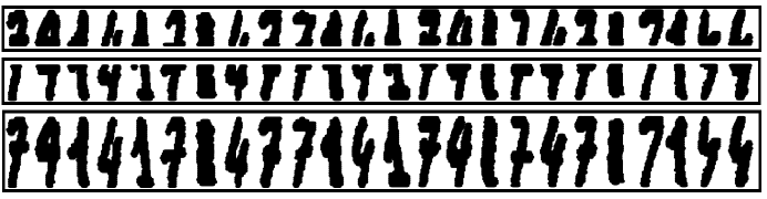
Figure 6: The first row consists of the responses $Y$ which are the upper halves of the image digits $\{1,4,7\}$; The second row consists of the predictors $X$ which are the bottom halves of the image digits $\{1,4,7\}$; The third row consists of the whole image digits $\{1,4,7\}$.

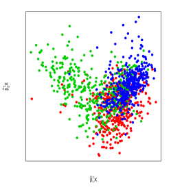
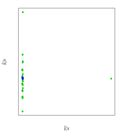
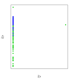
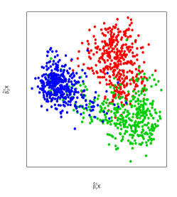
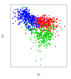
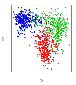
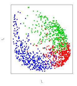
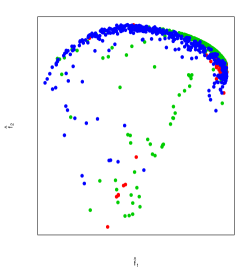
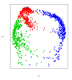
Figure 7: The first row consists of the scatter plots for the training data via projective resampling based SIR, SAVE and DR, respectively. The second row consists of the scatter plots based on our linear proposal with Euclidean distance, LLE and Isomap, respectively. The third row consists of the scatter plots based on our nonlinear proposal with Euclidean distance, LLE and Isomap, respectively. (red: $1$; green: $4$;blue: $7$.)

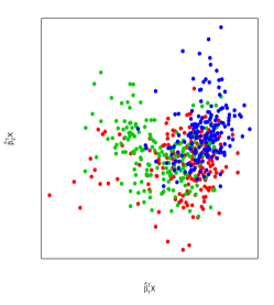
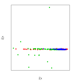
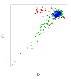
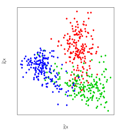
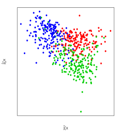
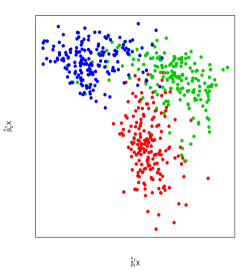
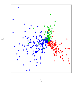
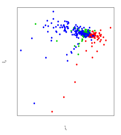
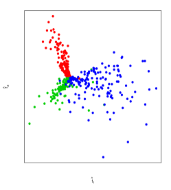
Figure 8: The first row consists of the perspective plots for the first two sufficient predictors for the testing data by SIR, SAVE and DR, respectively. The second row consists of the perspective plots for the testing data based on our linear proposal with Euclidean distance, LLE and Isomap, respectively. The third row consists of the perspective plots for our nonlinear proposal with Euclidean distance, LLE and Isomap, respectively. (red: $1$; green: $4$;blue: $7$.)

For image digits $\{1,4,7\}$, we also include projective resampling approach in combination with three classical methods, sliced inverse regression, sliced average variance estimation and directional regression for comparisons. And we adopt three different distance metrics for our proposals: the Euclidean distance, the distance metric learned by the Local Linear Embedding (Roweis & Saul (2000)), the distance metric learned by the Isomap approach (Tenenbaum et al. (2009)). Similar to the conclusion drawn from the application to image digits $\{0,8,9\}$, we again find that our proposals provide valid and useful information for classification as seen from Figure 2 and 3, especially for the nonlinear approach in combination with Isomap.

B.2 Structural Dimension Determination

Figure 9: The vertical axis in the panel (a) and (b) represents a combination of the measures about eigenvalues and eigenvectors, $g_{n}(k)$, for digits groups: {0,8,9} and {1,4,7}, respectively.

(a) The ladle plot

(b) The ladle plot

For the handwritten digits data, we apply the ladle estimator with the distance metric learned by the Isomap method. Figure 4 displays the ladle plot for digits $\{0,8,9\}$ and $\{1,4,7\}$ respectively. We find that in both cases the ladle estimator yields $\hat{d}=3$ or $4$. And from the scatter plots accumulated, we know that the first two sufficient predictors already provide useful information for image digits separation.

Appendix C Proofs of Theoretical Results

C.1 Proof of Proposition 1

Proposition 6.

$\Lambda$ is positive semidefinite. Assume the linearity condition holds true, then

$$\textup{Span}\left\{\Sigma^{-1}\Lambda\right\}\subseteq\mathcal{S}_{Y|X}.$$

Proof.

To prove the proposition, we introduction a fact that exists a separable $\mathbb{R}$-Hilbert space $\mathcal{H}$ and a mapping $\phi:\Omega\rightarrow\mathcal{H}$ such that $\forall Y,Y^{\prime}\in\mathcal{H}$, $d(Y,Y^{\prime})=\|\phi(Y)-\phi(Y^{\prime})\|^{2}_{\mathcal{H}}$, as shown by Schoenberg (1937, 1938). Let $\beta_{\phi}(\mu)=E\phi(Y)$. For $\forall a\in\mathbb{R}^{p},a\neq(0,\ldots,0)^{T}$, we have

$$a^{T}\Lambda a = -E\{\langle a^{T}(X-EX),a^{T}(X^{\prime}-EX)\rangle d(Y,Y^{\prime})\}$$

$$= -E\{\langle a^{T}(X-EX),a^{T}(X^{\prime}-EX)\rangle\|\phi(Y)-\phi(Y^{\prime})\|^{2}\}$$

$$= -E\{\langle a^{T}(X-EX),a^{T}(X^{\prime}-EX)\rangle\langle\phi(Y)-\phi(Y^{\prime}),\phi(Y)-\phi(Y^{\prime})\rangle\}$$

$$= -E\{\langle a^{T}(X-EX),a^{T}(X^{\prime}-EX)\rangle\langle\phi(Y)-\beta_{\phi}(\mu)+\beta_{\phi}(\mu)-\phi(Y^{\prime}),$$

$$\phi(Y)-\beta_{\phi}(\mu)+\beta_{\phi}(\mu)-\phi(Y^{\prime})\rangle\}$$

$$= 2E\{\langle a^{T}(X-EX),a^{T}(X^{\prime}-EX)\rangle\langle\phi(Y)-\beta_{\phi}(\mu),\phi(Y^{\prime})-\beta_{\phi}(\mu)\rangle\}$$

$$= 2\{E[a^{T}(X-EX)\otimes(\phi(Y)-\beta_{\phi}(\mu)]\}^{2}\geq 0$$

Therefore, $\Lambda$ is a semidefined matrix. By double expectation, we have

$$-\Sigma^{-1}E((X-EX)(X^{\prime}-EX)^{T}d(Y,Y^{\prime}))$$

$$= -\Sigma^{-1}E(E(X-E(X|Y))E(X^{\prime}-E(X|Y^{\prime}))^{T}d(Y,Y^{\prime})),$$

By the property of SIR, we have $\Sigma^{-1}E(X-E(X|Y))\in\mathcal{S}_{Y|X}$. The proof is completed.    

C.2 Proof of Theorem 1

Theorem 4.

Assume the linearity condition and the singular values $\lambda_{\ell}$’s are distinct for $\ell=1,\ldots,d$. In addition, assume that $Ed^{2}(Y,Y^{\prime})<\infty$ and $X$ has finite fourth moment, then

$$n^{1/2}(\hat{\beta}_{\ell}-\beta_{\ell})\overset{D}{\longrightarrow}N\left({0}_{p},\Sigma_{\ell}\right),$$ (C.10)

as $n\rightarrow\infty$, where $\Sigma_{\ell}=cov\{\Upsilon_{\ell}(X,Y)\}$.

The following lemmas are needed before we prove Theorem 1. Let $E(X)=\mu,\overline{X}=n^{-1}\sum_{i=1}^{n}X_{i}$ and $\widehat{\Sigma}=n^{-1}\sum_{i=1}^{n}(X_{i}-\overline{X})(X_{i}-\overline{X})^{T}$. Lemma 1 provides the asymptotic expansion of $\widehat{\Sigma}$. Its proof is obvious and thus omitted.

Lemma 1.

Assume $X$ has finite fourth moment. Then

$$\widehat{\Sigma}-\Sigma=\frac{1}{n}\sum\limits_{i=1}^{n}\Gamma(X_{i})+o_{P}(n^{-1/2}),$$ (C.11)

where $\Gamma(X_{i})=(X_{i}-\mu)(X_{i}-\mu)^{T}-\Sigma$.

Let $\Lambda=-E\{(X-\mu)(X^{\prime}-\mu)^{T}d(Y,Y^{\prime})\}$ and

$$\widehat{\Lambda}=-\frac{1}{n(n-1)}\sum_{1\leq i\neq j\leq n}(X_{i}-\overline{X})(X_{j}-\overline{X})^{T}d(Y_{i},Y_{j}).$$ (C.12)

Lemma 2 provides the asymptotic expansion of $\widehat{\Lambda}$.

Lemma 2.

Assume $X$ has finite fourth moment. Then

$$\widehat{\Lambda}-\Lambda=\frac{1}{n}\sum\limits_{i=1}^{n}\Theta(X_{i},Y_{i})+o_{P}(n^{-1/2}),$$ (C.13)

where the exact form of $\Theta(X_{i},Y_{i})$ is provided in the proof.

Proof.

First we decompose $\widehat{\Lambda}$ in (C.12) as $\widehat{\Lambda}=\widehat{U}^{(1)}+\widehat{U}^{(2)}+\widehat{U}^{(3)}+\widehat{U}^{(4)}$, where

$$\widehat{U}^{(1)} =-\frac{1}{n(n-1)}\sum_{i\neq j}(X_{i}-\mu)(X_{j}-\mu)^{T}d(Y_{i},Y_{j}),$$ (C.14)

$$\widehat{U}^{(2)} =\frac{1}{n(n-1)}\sum_{i\neq j}(\widehat{\mu}-\mu)(X_{j}-\mu)^{T}d(Y_{i},Y_{j}),$$

$$\widehat{U}^{(3)} =\frac{1}{n(n-1)}\sum_{i\neq j}(X_{i}-\mu)(\widehat{\mu}-\mu)^{T}d(Y_{i},Y_{j}),\text{ and}$$

$$\widehat{U}^{(4)} =-\frac{1}{n(n-1)}\sum_{i\neq j}(\widehat{\mu}-\mu)(\widehat{\mu}-\mu)^{T}d(Y_{i},Y_{j}).$$

Let $\Lambda^{(1)}(X_{i},Y_{i},X_{j},Y_{j})=-(X_{i}-\mu)(X_{j}-\mu)^{T}d(Y_{i},Y_{j})$ and denote $\Lambda^{(1)}_{1}(x,y)=E\{\Lambda^{(1)}(X,Y,x,y)\}$. For the first term, we have

$$\widehat{U}^{(1)}-\Lambda =\frac{1}{n(n-1)}\sum_{i\neq j}\{\Lambda^{(1)}(X_{i},Y_{i},X_{j},Y_{j})-\Lambda\}$$ (C.15)

$$=\frac{1}{n}\sum\limits_{i=1}^{n}\{\Lambda^{(1)}_{1}(X_{i},Y_{i})-\Lambda\}+\frac{1}{n(n-1)}\sum_{i\neq j}A(X_{i},Y_{i})$$

where

$$A(X_{i},Y_{i},X_{j},Y_{j})=\{\Lambda^{(1)}(X_{i},Y_{i},X_{j},Y_{j})-\Lambda^{(1)}_{1}(X_{i},Y_{i})\}.$$

By simple calculation,

$$E\|\frac{1}{n(n-1)}\sum_{i\neq j}A(X_{i},Y_{i})\|^{2}_{F}$$

$$= tr(E(\frac{1}{n(n-1)}\sum_{i\neq j}A(X_{i},Y_{i},X_{j},Y_{j}))(\frac{1}{n(n-1)}\sum_{k\neq t}A(X_{k},Y_{k},X_{t},Y_{t})))$$

$$= \frac{n(n-1)(n-2)(n-3)}{n^{2}(n-1)^{2}}tr(E(A(X,Y,X^{\prime},Y^{\prime})A(X^{\prime\prime},Y^{\prime\prime},X^{\prime\prime\prime},Y^{\prime\prime\prime})))$$

$$+\frac{n(n-1)(n-2)}{n^{2}(n-1)^{2}}tr(E(A(X,Y,X^{\prime},Y^{\prime})A(X,Y,X^{\prime\prime},Y^{\prime\prime})))$$

$$+\frac{n(n-1)}{n^{2}(n-1)^{2}}tr(E(A(X,Y,X^{\prime},Y^{\prime})A(X,Y,X^{\prime},Y^{\prime})))$$

$$= \frac{n(n-1)(n-2)}{n^{2}(n-1)^{2}}tr(E(E(A(X,Y,X^{\prime},Y^{\prime})|X,Y)E(A(X,Y,X^{\prime\prime},Y^{\prime\prime})|X,Y)))$$

$$+\frac{1}{n(n-1)}tr(E(A(X,Y,X^{\prime},Y^{\prime})A(X,Y,X^{\prime},Y^{\prime})))$$

$$= \frac{1}{n(n-1)}tr(E(A(X,Y,X^{\prime},Y^{\prime})A(X,Y,X^{\prime},Y^{\prime})))=O(n^{-2})$$

we get $\frac{1}{n(n-1)}\sum_{i\neq j}A(X_{i},Y_{i})=O_{p}(n^{-1})$.

Let $\vartheta=E\{(X-\mu)d(Y,Y^{\prime})\}$. Note that

$$\frac{1}{n(n-1)}\sum\limits_{i\neq j}(X_{j}-\mu)d(Y_{i},Y_{j})\overset{P}{\longrightarrow}\vartheta.$$

It follows that

$$\widehat{U}^{(2)}=\frac{1}{n}\sum_{i=1}^{n}(X_{i}-\mu)\vartheta^{T}+o_{P}(n^{-1/2}).$$ (C.16)

Similarly we have

$$\widehat{U}^{(3)}=\frac{1}{n}\sum_{i=1}^{n}\vartheta(X_{i}-\mu)^{T}+o_{P}(n^{-1/2}).$$ (C.17)

Note that $\widehat{U}^{(4)}=o_{P}(n^{-1/2})$. (C.15), (C.16) and (C.17) together lead to (C.13), where $\Theta(X_{i},Y_{i})=\Lambda^{(1)}_{1}(X_{i},Y_{i})-\Lambda+(X_{i}-\mu)\vartheta^{T}+\vartheta(X_{i}-\mu)^{T}$.

By algebra calculations, we have

$$\widehat{M}-M = \widehat{\Sigma}^{-1}\widehat{\Lambda}-\Sigma^{-1}\Lambda=(\widehat{\Sigma}^{-1}-\Sigma^{-1})\Lambda+\Sigma^{-1}(\widehat{\Lambda}-\Lambda)+O_{p}(n^{-1})$$

$$= -\Sigma^{-1}(\widehat{\Sigma}-\Sigma)\Sigma^{-1}\Lambda+\Sigma^{-1}(\widehat{\Lambda}-\Lambda)+o_{p}(n^{-1/2})$$

$$= -\frac{1}{n}\sum_{i=1}^{n}\Sigma^{-1}((X_{i}-\mu)(X_{i}-\mu)^{T}-\Sigma)\Sigma^{-1}\Lambda$$

$$+\frac{1}{n(n-1)}\sum_{i\neq j}\Sigma^{-1}((X_{i}-\mu)(X_{j}-\mu)^{T}d(Y_{i},Y_{j})-\Lambda)$$

$$+\Sigma^{-1}(\mu-\bar{X})\vartheta^{T}+\Sigma^{-1}\vartheta(\mu-\bar{X})^{T}+o_{p}(n^{-1/2})$$

$$= -\frac{1}{n}\sum_{i=1}^{n}\Sigma^{-1}((X_{i}-\mu)(X_{i}-\mu)^{T}-\Sigma)\Sigma^{-1}\Lambda$$

$$+\frac{1}{n}\sum_{i=1}^{n}\Sigma^{-1}(\Lambda^{(1)}_{1}(X_{i},Y_{i})-\Lambda)$$

$$+\Sigma^{-1}(\mu-\bar{X})\vartheta^{T}+\Sigma^{-1}\vartheta(\mu-\bar{X})^{T}+o_{p}(n^{-1/2})$$

$$= \frac{1}{n}\sum_{i=1}^{n}H(X_{i},Y_{i})+o_{p}(n^{-1/2})$$

where

$$H(X,Y) = -\Sigma^{-1}((X-\mu)(X-\mu)^{T}$$

$$-\Sigma)\Sigma^{-1}\Lambda+\Sigma^{-1}(\Lambda^{(1)}_{1}(X,Y)-\Lambda)$$

$$+\Sigma^{-1}(\mu-X)\vartheta^{T}+\Sigma^{-1}\vartheta(\mu-X)^{T}$$

Simple calculations lead to

$$\widehat{M}\widehat{M}^{T}-MM^{T} = \Sigma^{-1}(\widehat{\Lambda}-\Lambda)\Lambda^{T}\Sigma^{-1}+(\widehat{\Sigma}^{-1}-\Sigma^{-1})\Lambda\Lambda^{T}\Sigma^{-1}$$

$$+\Sigma^{-1}\Lambda\Lambda^{T}(\widehat{\Sigma}^{-1}-\Sigma^{-1})+\Sigma^{-1}\Lambda(\widehat{\Lambda}-\Lambda)^{T}\Sigma^{-1}$$

Observe that $\lambda_{\ell}$ and $\beta_{\ell}$ satisfy the following singular value decomposition equation:

$$MM^{T}\beta_{\ell}=\lambda_{\ell}^{2}\beta_{\ell},\text{ and}\quad\ell=1,\ldots,p,$$

Hence,

$$\Sigma^{-1}\Lambda\Lambda^{T}\Sigma^{-1}\beta_{\ell}=\lambda_{\ell}^{2}\beta_{\ell},\text{ and}\quad\ell=1,\ldots,p,$$

where $\beta_{\ell}^{T}\beta_{\ell}=1$ and $\beta_{\ell}^{T}\beta_{\jmath}=0$ for $\ell\neq\jmath$. Similarly, in the sample level, we have

$$\widehat{\Sigma}^{-1}\widehat{\Lambda}\widehat{\Lambda}^{T}\widehat{\Sigma}^{-1}\beta_{\ell}=\lambda_{\ell}^{2}\beta_{\ell},\text{ and}\quad\ell=1,\ldots,p;$$

where $\beta_{\ell}^{T}\beta_{\ell}=1$ and $\beta_{\ell}^{T}\beta_{\jmath}=0$ for $\ell\neq\jmath$. The singular value decomposition form in the sample level implies that

$$\Sigma^{-1}(\widehat{\Lambda}-\Lambda)\Lambda^{T}\Sigma^{-1}\beta_{\ell}+(\widehat{\Sigma}^{-1}-\Sigma^{-1})\Lambda\Lambda^{T}\Sigma^{-1}\beta_{\ell}$$

$$+ \Sigma^{-1}\Lambda\Lambda^{T}(\widehat{\Sigma}^{-1}-\Sigma^{-1})\beta_{\ell}+\Sigma^{-1}\Lambda(\widehat{\Lambda}-\Lambda)^{T}\Sigma^{-1}\beta_{\ell}+\Sigma^{-1}\Lambda\Lambda^{T}\Sigma^{-1}(\widehat{\beta}_{\ell}-\beta_{\ell})$$

$$= \lambda_{\ell}(\widehat{\lambda}_{\ell}-\lambda_{\ell})\beta_{\ell}+(\widehat{\lambda}_{\ell}-\lambda_{\ell})\lambda_{\ell}\beta_{\ell}+\lambda_{\ell}^{2}(\widehat{\beta}_{\ell}-\beta_{\ell})+o_{p}(n^{-1/2})$$

for $\ell=1,\ldots,p$. Multiply both sides of (C.2) by $\beta^{T}_{\ell}$, we get from the left

$$\beta^{T}_{\ell}[\Sigma^{-1}(\widehat{\Lambda}-\Lambda)\Lambda^{T}\Sigma^{-1}+(\widehat{\Sigma}^{-1}-\Sigma^{-1})\Lambda\Lambda^{T}\Sigma^{-1}+\Sigma^{-1}\Lambda\Lambda^{T}(\widehat{\Sigma}^{-1}-\Sigma^{-1})$$

$$+ \Sigma^{-1}\Lambda(\widehat{\Lambda}-\Lambda)^{T}\Sigma^{-1}]\beta_{\ell}=\lambda_{\ell}(\widehat{\lambda}_{\ell}-\lambda_{\ell})+(\widehat{\lambda}_{\ell}-\lambda_{\ell})\lambda_{k}+o_{p}(n^{-1/2})$$

which further suggests that

$$\widehat{\lambda}_{\ell} = \lambda_{\ell}+\frac{\beta^{T}_{\ell}}{2\lambda_{\ell}}[\Sigma^{-1}(\widehat{\Lambda}-\Lambda)\Lambda^{T}\Sigma^{-1}+(\widehat{\Sigma}^{-1}-\Sigma^{-1})\Lambda\Lambda^{T}\Sigma^{-1}$$

$$+ \Sigma^{-1}\Lambda\Lambda^{T}(\widehat{\Sigma}^{-1}-\Sigma^{-1})+\Sigma^{-1}\Lambda(\widehat{\Lambda}-\Lambda)^{T}\Sigma^{-1}]\beta_{\ell}+o_{p}(n^{-1/2})$$

By lemma A.2 of Cook & Ni (2005), we know that

$$\widehat{\Sigma}^{-1}-\Sigma^{-1}=-\Sigma^{-1}(\widehat{\Sigma}-\Sigma)\Sigma^{-1}+o_{p}(n^{-1/2})$$

Hence, equation (C.2) becomes

$$\widehat{\lambda}_{\ell} = \lambda_{\ell}+\frac{\beta^{T}_{\ell}}{2\lambda_{\ell}}[\Sigma^{-1}(\widehat{\Lambda}-\Lambda)\Lambda^{T}\Sigma^{-1}-\Sigma^{-1}(\widehat{\Sigma}-\Sigma)\Sigma^{-1}\Lambda\Lambda^{T}\Sigma^{-1}$$

$$- \Sigma^{-1}\Lambda\Lambda^{T}\Sigma^{-1}(\widehat{\Sigma}-\Sigma)\Sigma^{-1}+\Sigma^{-1}\Lambda(\widehat{\Lambda}-\Lambda)^{T}\Sigma^{-1}]\beta_{\ell}+o_{p}(n^{-1/2})$$

$$= \lambda_{\ell}+\frac{1}{n}\sum_{i=1}^{n}C_{i,\lambda_{\ell}}+o_{p}(n^{-1/2})$$

where

$$C_{i,\lambda_{\ell}} = \frac{\beta^{T}_{\ell}}{2\lambda_{\ell}}[\Sigma^{-1}\Theta(X_{i},Y_{i})\Lambda^{T}\Sigma^{-1}-\Sigma^{-1}\Gamma(X_{i})\Sigma^{-1}\Lambda\Lambda^{T}\Sigma^{-1}$$

$$- \Sigma^{-1}\Lambda\Lambda^{T}\Sigma^{-1}\Gamma(X_{i})\Sigma^{-1}+\Sigma^{-1}\Lambda\Theta(X_{i},Y_{i})\Sigma^{-1}]\beta_{\ell}+o_{p}(n^{-1/2})$$

Now we return to the expansion of $\hat{\beta}_{\ell}$. Since $(\beta_{1},\ldots,\beta_{p})$ is a basis if $R^{p}$, there exists $c_{\ell j}$ for $j=1,\ldots,p$, such that $\widehat{\beta}_{\ell}-\beta_{\ell}=\sum_{j=1}^{p}c_{\ell j}\beta_{j}$ and $c_{\ell j}=O_{p}(n^{-1/2})$. We will derive the explicit form of $c_{\ell j}$ in the next step. Note that (C.2) can be rewritten as

$$(\Sigma^{-1}\Lambda\Lambda^{T}\Sigma^{-1}-\lambda_{\ell}^{2})\sum_{j=1}^{p}c_{\ell j}\beta_{j}$$

$$= \lambda_{\ell}(\widehat{\lambda}_{\ell}-\lambda_{\ell})\beta_{\ell}+(\widehat{\lambda}_{\ell}-\lambda_{\ell})\lambda_{\ell}\beta_{\ell}+[\Sigma^{-1}(\widehat{\Lambda}-\Lambda)\Lambda^{T}\Sigma^{-1}$$

$$+ (\widehat{\Sigma}^{-1}-\Sigma^{-1})\Lambda\Lambda^{T}\Sigma^{-1}+\Sigma^{-1}\Lambda\Lambda^{T}(\widehat{\Sigma}^{-1}-\Sigma^{-1})+\Sigma^{-1}\Lambda(\widehat{\Lambda}-\Lambda)^{T}\Sigma^{-1}]\beta_{\ell}$$

$$= \lambda_{\ell}(\widehat{\lambda}_{\ell}-\lambda_{\ell})\beta_{\ell}+(\widehat{\lambda}_{\ell}-\lambda_{\ell})\lambda_{\ell}\beta_{\ell}+[\Sigma^{-1}(\widehat{\Lambda}-\Lambda)\Lambda^{T}\Sigma^{-1}$$

$$- \Sigma^{-1}(\widehat{\Sigma}-\Sigma)\Sigma^{-1}\Lambda\Lambda^{T}\Sigma^{-1}-\Sigma^{-1}\Lambda\Lambda^{T}\Sigma^{-1}(\widehat{\Sigma}-\Sigma)\Sigma^{-1}+\Sigma^{-1}\Lambda(\widehat{\Lambda}-\Lambda)^{T}\Sigma^{-1}]\beta_{\ell}$$

$$= \lambda_{\ell}(\widehat{\lambda}_{\ell}-\lambda_{\ell})\beta_{\ell}+(\widehat{\lambda}_{\ell}-\lambda_{\ell})\lambda_{\ell}\beta_{\ell}+\frac{1}{n}\sum_{1=1}^{n}\zeta_{\ell}(X_{i},Y_{i})\beta_{\ell}$$

where

$$\zeta_{\ell}(X_{i},Y_{i}) = \Sigma^{-1}\Theta(X_{i},Y_{i})\Lambda\Sigma^{-1}-\Sigma^{-1}\Gamma(X_{i})\Sigma^{-1}\Lambda\Lambda^{T}\Sigma^{-1}$$

$$- \Sigma^{-1}\Lambda\Lambda^{T}\Sigma^{-1}\Gamma(X_{i})\Sigma^{-1}+\Sigma^{-1}\Lambda\Theta(X_{i},Y_{i})\Sigma^{-1}$$

Multiply both sides of (C.2) by $\beta_{j}^{T}\ (j\neq\ell)$, we can get from the left

$$c_{\ell,j}=\frac{1}{n}\sum_{i=1}\frac{\beta_{j}^{T}\zeta_{\ell}(X_{i},Y_{i})\beta_{\ell}}{\lambda_{j}^{2}-\lambda_{\ell}^{2}},\ j\neq\ell;$$ (C.22)

In addition, $\beta_{\ell}^{T}\beta_{\ell}=\widehat{\beta}_{\ell}^{T}\widehat{\beta}_{\ell}=1$ indicates that

$$0={\sum_{j=1}^{p}c_{\ell j}\beta^{T}_{j}}\beta_{\ell}+\beta_{\ell}^{T}{\sum_{j=1}^{p}c_{\ell j}\beta_{j}},$$

which further implies that $c_{\ell\ell}=0$. We define

$$\Sigma_{\ell}=\mathrm{cov}(\Upsilon_{\ell}(X,Y)),$$ (C.23)

where $p\times 1$ random vector $\Upsilon_{\ell}(X,Y)=\sum_{j=1,j\neq\ell}^{p}\frac{\beta_{j}\beta_{j}^{T}\zeta_{\ell}(X,Y)\beta_{\ell}}{\lambda_{j}^{2}-\lambda_{\ell}^{2}}.$ Then plug (C.22) and (C.11) into (C.13), and we get

$$\widehat{\beta}_{\ell}=\beta_{\ell}+\frac{1}{n}\sum_{i=1}^{n}\Upsilon_{\ell}(X_{i},Y_{i})+o_{p}(n^{-1/2})$$ (C.24)

The conclusion is then straightforward via the central limit theorem.    

C.3 Proof of Theorem 2

Theorem 5.

Assume $Ed^{2}(Y,Y^{\prime})<\infty$ and $X$ has finite fourth moment. And suppose Assumptions (1)–(2) hold, then

$$P_{r}\{\lim_{n\rightarrow\infty}P_{r}(\hat{d}=d|\mathcal{D}){=1}\}=1,$$

where $\mathcal{D}=\{(X_{1},Y_{1}),(X_{2},Y_{2}),\ldots\}$ is a sequence of independent copies of $(X,Y)$.

Proof.

The singular value of $\widehat{M}$ are square root of the corresponding eigenvalue of matrix $\widehat{M}\widehat{M}^{T}$. Moreover, the left singular vectors are the same as the eigenvectors of $\widehat{M}\widehat{M}^{T}$. Then we apply Theorem 2 in Luo & Li (2016) to get the desired result.    

C.4 Proof of Proposition 2

Proposition 7.

$\Lambda_{XX^{\prime}}$ is a bounded linear and self-adjoint operator. For any $f,g\in\mathcal{H}_{X}$,

$$\langle f,\Lambda_{XX^{\prime}}g\rangle_{\mathcal{H}_{X}}=-E\{(f(X)-Ef(X))(g(X^{\prime})-E{g(X^{\prime})})d(Y,Y^{\prime})\}.$$

Moreover, there exists a separable $\mathbb{R}$-Hilbert space $\mathcal{H}$ and a mapping $\phi:\Omega\rightarrow\mathcal{H}$ such that

$$\langle f,\Lambda_{XX^{\prime}}f\rangle_{\mathcal{H}_{X}}=2\{E[(f(X)-Ef(X))(\phi(Y)-E\phi(Y))]\}^{2}=2(cov[f(X),\phi(Y)])^{2},$$

Proof.

For arbitrary $f,g\in\mathcal{H}_{X}$, we have

$$|\langle f,\Lambda_{XX^{\prime}}g\rangle_{\mathcal{H}_{X}}| \leq E|\langle f,((\kappa_{X}(\cdot,X)-\mu_{X})\otimes(\kappa_{X}(\cdot,X^{\prime})-\mu_{X})d(Y,Y^{\prime}))g\rangle_{\mathcal{H}_{X}}|$$

$$= E\{|\langle f,\kappa_{X}(\cdot,X)-\mu_{X}\rangle_{\mathcal{H}_{X}}||\langle\kappa_{X}(\cdot,X^{\prime})-\mu_{X},g\rangle_{\mathcal{H}_{X}}|d(Y,Y^{\prime})\}$$

$$\leq \|f\|_{\mathcal{H}_{X}}\|g\|_{\mathcal{H}_{X}}E\langle\kappa_{X}(\cdot,X)-\mu_{X},\kappa_{X}(\cdot,X)-\mu_{X}\rangle_{\mathcal{H}_{X}}(Ed^{2}(Y,Y^{\prime}))^{1/2}$$

$$= \|f\|_{\mathcal{H}_{X}}\|g\|_{\mathcal{H}_{X}}(E\kappa_{X}(X,X)-\mu_{X}^{2})(Ed^{2}(Y,Y^{\prime}))^{1/2}$$

Since

$$\mu_{X}^{2}\leq(E\|\kappa_{X}(\cdot,X)\|_{\mathcal{H}_{X}})^{2}=(E\kappa_{X}(X,X)^{1/2})^{2}\leq E\kappa_{X}(X,X)<\infty,$$

and $Ed^{2}(Y,Y^{\prime})<\infty$. Therefore, $\Lambda_{XX^{\prime}}$ is a bounded liner and self-adjoint operator.

$$\langle f,\Lambda_{XX^{\prime}}g\rangle_{\mathcal{H}_{X}} = -E\langle f,((\kappa_{X}(\cdot,X)-\mu_{X})\otimes(\kappa_{X}(\cdot,X^{\prime})-\mu_{X})d(Y,Y^{\prime}))g\rangle_{\mathcal{H}_{X}}$$

$$= -E\{\langle f,\kappa_{X}(\cdot,X)-\mu_{X}\rangle_{\mathcal{H}_{X}}\langle\kappa_{X}(\cdot,X^{\prime})-\mu_{X},g\rangle_{\mathcal{H}_{X}}d(Y,Y^{\prime})\}$$

$$= -E\{(f(X)-Ef(X))(g(X^{\prime})-E{g(X^{\prime})})d(Y,Y^{\prime})\}$$

For arbitrary $f\in\mathcal{H}_{X}$, we have

$$\langle f,\Lambda_{XX^{\prime}}f\rangle_{\mathcal{H}_{X}} = -\langle f,E((\kappa_{X}(\cdot,X)-\mu_{X})\otimes(\kappa_{X}(\cdot,X^{\prime})-\mu_{X})d(Y,Y^{\prime}))f\rangle_{\mathcal{H}_{X}}$$

$$= -E\{\langle f,((\kappa_{X}(\cdot,X)-\mu_{X})\otimes(\kappa_{X}(\cdot,X^{\prime})-\mu_{X}))f\rangle_{\mathcal{H}_{X}}\|\phi(Y)-\phi(Y^{\prime})\|_{\mathcal{H}}^{2}\}$$

$$= 2E\{\langle f(X)-Ef(X),f(X^{\prime})-Ef(X^{\prime})\rangle_{\mathcal{H}_{X}}\langle\phi(Y)-\beta_{\phi}(\mu),\phi(Y^{\prime})-\beta_{\phi}(\mu)\rangle_{\mathcal{H}}\}$$

$$= 2\{E(f(X)-Ef(X))\otimes(\phi(Y)-\beta_{\phi}(\mu))\}^{2}\geq 0$$

Therefore, $\Lambda_{XX^{\prime}}$ is a semidefined operator.    

C.5 Proof of Proposition 3

Proposition 8.

Suppose assumptions (3)–(5) hold, then

$$\overline{\textup{ran}}\left\{\Sigma_{XX}^{-1}\Lambda_{XX^{\prime}}\right\}\subseteq\mathcal{G}_{Y|X}.$$

Proof.

Firstly, we show that

$$\overline{\mathrm{ran}}(\Lambda_{XX^{\prime}})\subseteq\Sigma_{XX}\mathcal{G}_{Y|X}$$

which is equivalent to

$$(\Sigma_{XX}\mathcal{G}_{Y|X})^{\bot}\subseteq\overline{\mathrm{ran}}(\Lambda_{XX^{\prime}})^{\bot}.$$

Since $\overline{\mathrm{ran}}(\Lambda_{XX^{\prime}})^{\bot}=\ker(\Lambda_{XX^{\prime}})$, where $\ker(\Lambda_{XX^{\prime}})$ denotes nuclear space generated by the operator $\Lambda_{XX^{\prime}}$, it suffices to show that

$$(\Sigma_{XX}\mathcal{G}_{Y|X})^{\bot}\subseteq\ker(\Lambda_{XX^{\prime}}).$$

Now we define $\mathcal{G}_{\phi(Y)|X}$, we get

$$(\Sigma_{XX}\mathcal{G}_{\phi(Y)|X})^{\bot}\subseteq\ker(\Lambda_{XX^{\prime}}).$$ (C.25)

Let $f\in(\Sigma_{XX}\mathcal{G}_{\phi(Y)|X})^{\bot}$. Then, for all $g\in\mathcal{G}_{\phi(Y)|X}$, we have

$$\langle f,\Sigma_{XX}g\rangle_{\mathcal{H}_{X}}=cov\{f(X),g(X)\}=0.$$

Because $g$ is measurable with respect to $\mathcal{M}_{\phi(Y)|X}$, we have $g(X)=E[g(X)|\mathcal{M}_{\phi(Y)|X}]$. And

$$cov\{f(X),E[g(X)|\mathcal{M}_{\phi(Y)|X}]\}$$

$$= E[f(X)E[g(X)|\mathcal{M}_{\phi(Y)|X}]]-E[f(X)]E[g(X)]$$

$$= E[E[f(X)|\mathcal{M}_{\phi(Y)|X}]g(X)]-E[f(X)]E[g(X)]$$

$$= cov\{E[f(X)|\mathcal{M}_{\phi(Y)|X}],g(X)\}$$

The second equation is based on the property of double expectation. Since $\mathcal{G}_{\phi(Y)|X}$ is dense in $L_{2}(P_{X}|\mathcal{M}_{\phi(Y)|X})$ modulo constants, there exists a sequence $\{f_{n}\subseteq\mathcal{G}_{\phi(Y)|X}\}$ such that $var[f_{n}(X)-f(X)]\rightarrow 0$. Then

$$cov\{E[f(X)|\mathcal{M}_{\phi(Y)|X}],f_{n}(X)\}=E\{E[f(X)|\mathcal{M}_{\phi(Y)|X}]f_{n}(X)\}-E[f(X)]E[f_{n}(X)]=0$$ (C.26)

On the other hand,

$$cov\{E[f(X)|\mathcal{M}_{\phi(Y)|X}],f_{n}(X)\} \rightarrow cov\{E[f(X)|\mathcal{M}_{\phi(Y)|X}],f(X)\}$$

$$= cov\{E[f(X)|\mathcal{M}_{\phi(Y)|X}],E[f(X)|\mathcal{M}_{\phi(Y)|X}]\}$$

Combining (C.26) and (C.5), we have

$$var\{E[f(X)|\mathcal{M}_{\phi(Y)|X}]\}=0$$

This implies that $E[f(X)|\mathcal{M}_{\phi(Y)|X}]=$ constant almost surely. Since $\mathcal{M}_{\phi(Y)|X}$ is sufficient, we have $E[f(X)|\mathcal{M}_{\phi(Y)|X}]=E[f(X)|\phi(Y),\mathcal{M}_{\phi(Y)|X}]$. So $E[f(X)|\phi(Y),\mathcal{M}_{\phi(Y)|X}]=$ constant almost surely. Consequently, $E[f(X)|\phi(Y)]=$ constant almost surely.

$$\Sigma^{-1}_{XX}E[(\kappa_{X}(\cdot,X)-\mu_{X})\otimes(\kappa_{X}(\cdot,X^{\prime})-\mu_{X})d(Y,Y^{\prime})]$$

$$= \Sigma^{-1}_{XX}E[(\kappa_{X}(\cdot,X)-\mu_{X})\otimes(\kappa_{X}(\cdot,X^{\prime})-\mu_{X})\|\phi(Y)-\phi(Y^{\prime})\|^{2}_{\mathcal{H}}]$$

$$= \Sigma^{-1}_{XX}E\{E[(\kappa_{X}(\cdot,X)-\mu_{X})|\phi(Y)]\otimes E[(\kappa_{X}(\cdot,X^{\prime})-\mu_{X})|\phi(Y^{\prime})]\|\phi(Y)-\phi(Y^{\prime})\|^{2}_{\mathcal{H}}]\}$$

We can get

$$E[(\kappa_{X}(\cdot,X^{\prime})-\mu_{X})|\phi(Y^{\prime})]f=E[f(X^{\prime}))|\phi(Y^{\prime})]-\mu_{X}(f(X^{\prime}))=0$$

Therefore, $\Lambda_{XX^{\prime}}f=0$. Then we have proved (C.25).

By (C.25), we have

$${ran}(\Lambda_{XX^{\prime}})\subseteq\Sigma_{XX}\mathcal{G}_{\phi(Y)|X},$$

which implies $\Sigma^{-1}_{XX}\mathrm{ran}(\Lambda_{XX^{\prime}})\subseteq\mathcal{G}_{\phi(Y)|X}$. Note that

$$\Sigma^{-1}_{XX}\mathrm{ran}(\Lambda_{XX^{\prime}}) = \{\Sigma^{-1}_{XX}f:f=\Lambda_{XX^{\prime}}g,g\in\mathcal{H}_{\phi(Y)}\}$$

$$= \{\Sigma^{-1}_{XX}\Lambda_{XX^{\prime}}g:g\in\mathcal{H}_{\phi(Y)}\}=\mathrm{ran}(\Sigma^{-1}_{XX}\Lambda_{XX^{\prime}})$$

Then, because $\mathcal{G}_{\phi(Y)|X}$ is closed, we have $\overline{\mathrm{ran}}(\Sigma^{-1}_{XX}\Lambda_{XX^{\prime}})\subseteq\mathcal{G}_{\phi(Y)|X}.$

Finally, we will show $\mathcal{G}_{\phi(Y)|X}\subseteq\mathcal{G}_{Y|X}$. It is easy to find that

$$Y\;\,\rule[0.0pt]{0.29999pt}{6.69998pt}\rule[0.0pt]{6.49994pt}{0.29999pt}\rule[0.0pt]{0.29999pt}{6.69998pt}\;\,X|\mathcal{G}_{Y|X}\Rightarrow\phi(Y)\;\,\rule[0.0pt]{0.29999pt}{6.69998pt}\rule[0.0pt]{6.49994pt}{0.29999pt}\rule[0.0pt]{0.29999pt}{6.69998pt}\;\,X|\mathcal{G}_{\phi(Y)|X}$$

Therefore, we have $\mathcal{G}_{\phi(Y)|X}\subseteq\mathcal{G}_{Y|X}.$ The proof is completed.    

C.6 Proof of Proposition 4

Proposition 9.

Suppose assumptions (3)–(5) hold and $\mathcal{G}_{Y|X}$ is complete. Then,

$$\overline{\textup{ran}}\left\{\Sigma_{XX}^{-1}\Lambda_{XX^{\prime}}\right\}=\mathcal{G}_{Y|X}.$$

Proof.

Form Proposition 8, we know $\overline{\mathrm{ran}}(\Lambda_{XX^{\prime}})\subseteq\Sigma_{XX}\mathcal{G}_{Y|X}$. Therefore, we only need to show $\Sigma_{XX}\mathcal{G}_{Y|X}\subseteq\overline{\mathrm{ran}}(\Lambda_{XX^{\prime}})$, or equivalently, $\mathrm{ker}(\Lambda_{X^{\prime}X})\subseteq(\Sigma_{XX}\mathcal{G}_{Y|X})^{\perp}$. Let $f\in\mathrm{ker}(\Lambda_{X^{\prime}X})$. Then $\Lambda_{X^{\prime}X}f=0$, which implies that $\Sigma^{-1}_{X^{\prime}X^{\prime}}\Lambda_{X^{\prime}X}f=0$. By the proof of Proposition 8, we have $E(f(X)|\mathcal{M}_{\phi(Y)|X})=\mathrm{constant}$. Since $\mathcal{M}_{\phi(Y)|X}\subseteq\mathcal{M}_{Y|X}$, we have $E(f(X)|\mathcal{M}_{Y|X})=\mathrm{constant}$. It follows that, for any $g\in\Sigma_{XX}\mathcal{G}_{Y|X}$, we have

$$cov(f(X),g(X))=cov(f(X),E(g(X)|\mathcal{M}_{Y|X}))=cov(E(f(X)|\mathcal{M}_{Y|X}),g(X))=0.$$

That is, $f\in(\Sigma_{XX}\mathcal{G}_{Y|X})^{\perp}$. The proof is completed.    

C.7 Proof of Theorem 3

Theorem 6.

Suppose assumptions (3)–(7) hold. In addition, assume that $Ed^{2}(Y,Y^{\prime})<\infty$, then as $n\rightarrow\infty$

$$\|\hat{V}_{XX^{\prime}}-V_{XX^{\prime}}\|_{HS}=o_{p}(1),\ \ \ |\langle\hat{\psi}_{1},\psi_{1}\rangle_{\text{HS}}|\stackrel{{\scriptstyle P}}{{\longrightarrow}}1,$$

$$\|\{\hat{f}_{1}(X)-E\hat{f}_{1}(X)\}-\{f_{1}(X)-Ef_{1}(X)\}\|{\longrightarrow}0,$$

where $\|\cdot\|$ in this theorem is the standard $L_{2}$ norm to measure the distance of functions and $\|\cdot\|_{\text{HS}}$ denotes the Hilbert-Schmidt norm.

To prove this theorem, we need the following lemmas.

Lemma 3.

The cross-covariance operator $\Lambda_{XX^{\prime}}$ is a Hilbert-Schmidt operator, and its Hilbert-Schmidt norm is given by

$$\|\Lambda_{XX^{\prime}}\|^{2}_{\text{HS}} = \langle E\{(\kappa_{X}(,X)-\mu_{X})\otimes(\kappa_{X}(,X^{\prime})-\mu_{X})d(Y,Y^{\prime})\},$$

$$E\{(\kappa_{X}(,X)-\mu_{X})\otimes(\kappa_{X}(,X^{\prime})-\mu_{X})d(Y,Y^{\prime})\}\rangle$$

$$= E_{XX^{\prime}YY^{\prime}}E_{X^{\prime\prime}X^{\prime\prime\prime}Y^{\prime\prime}Y^{\prime\prime\prime}}[\langle(\kappa_{X}(,X)-\mu_{X}),(\kappa_{X}(,X^{\prime\prime})-\mu_{X})\rangle_{\mathcal{H}_{X}}$$

$$\langle(\kappa_{X}(,X^{\prime})-\mu_{X}),(\kappa_{X}(,X^{\prime\prime\prime})-\mu_{X})\rangle_{\mathcal{H}_{X}}d(Y,Y^{\prime})d(Y^{\prime\prime},Y^{\prime\prime\prime})]$$

$$= \|E_{XX^{\prime}YY^{\prime}}[(\kappa_{X}(,X)-\mu_{X})(\kappa_{X}(,X^{\prime})-\mu_{X})d(Y,Y^{\prime})]\|_{\mathcal{H}_{X}\otimes\mathcal{H}_{X}}^{2}$$

where $(X,Y)$,$(X^{\prime},Y^{\prime})$,$(X^{\prime\prime},Y^{\prime\prime})$ and $(X^{\prime\prime\prime},Y^{\prime\prime\prime})$ are independently and identically with distribution $P_{XY}$.

From the facts $\mathcal{H}_{X}\subset L_{2}(P_{X})$, the law of large numbers implies for each $f\in\mathcal{H}_{X}$,

$$\lim_{n\rightarrow\infty}\langle f,\widehat{\Lambda}_{XX^{\prime}}f\rangle_{\mathcal{H}_{X}}=\langle f,\Lambda_{XX^{\prime}}f\rangle_{\mathcal{H}_{X}}$$

in probability. Moreover, the central limit theorem shows that the above convergence rate is of order $O_{p}(n^{-1/2})$. The following lemma shows the tight uniform result that $\|\widehat{\Lambda}_{XX^{\prime}}-\Lambda_{XX^{\prime}}\|_{HS}$ converges to zero in the order of $O_{p}(n^{-1/2})$.

Lemma 4.

Under the Assumption 3 and $Ed^{2}(Y,Y^{\prime})<\infty$, we have

$$\|\widehat{\Lambda}_{XX^{\prime}}-\Lambda_{XX^{\prime}}\|_{HS}=O_{p}(n^{-1/2})$$

Proof.

Write for simplicity $\eta=\kappa_{X}(\cdot,X)-\mu_{X}$ and $\mathcal{F}=\mathcal{H}_{X}\otimes\mathcal{H}_{X}$. Then $\eta_{1},\ldots,\eta_{n}$ are i.i.d. random elements in $\mathcal{H}_{X}$. Lemma 3 implies

$$\|\widehat{\Lambda}_{XX^{\prime}}\|^{2}_{HS} = \|\frac{1}{n(n-1)}\sum_{i\neq j}^{n}[(\eta_{i}-\frac{1}{n}\sum_{s=1}^{n}\eta_{s})(\eta_{j}-\frac{1}{n}\sum_{s=1}^{n}\eta_{s})d(Y_{i},Y_{j})]\|_{\mathcal{F}}^{2}.$$

Then we can derive that

$$\langle\Lambda_{XX^{\prime}},\widehat{\Lambda}_{XX^{\prime}}\rangle_{HS}$$

$$= \langle E[\eta\eta^{\prime}d(Y,Y^{\prime})],\frac{1}{n(n-1)}\sum_{i\neq j}^{n}[(\eta_{i}-\frac{1}{n}\sum_{s=1}^{n}\eta_{s})(\eta_{j}-\frac{1}{n}\sum_{s=1}^{n}\eta_{s})d(Y_{i},Y_{j})]\rangle_{\mathcal{F}}$$

From these equations, we have

$$\|\widehat{\Lambda}_{XX^{\prime}}-\Lambda_{XX^{\prime}}\|^{2}_{HS}$$

$$= \|\Lambda_{XX^{\prime}}\|^{2}_{HS}-2\langle\Lambda_{XX^{\prime}},\widehat{\Lambda}_{XX^{\prime}}\rangle_{HS}+\|\widehat{\Lambda}_{XX^{\prime}}\|^{2}_{HS}$$

$$= \|\frac{1}{n(n-1)}\sum_{i\neq j}^{n}[(\eta_{i}-\frac{1}{n}\sum_{s=1}^{n}\eta_{s})(\eta_{j}-\frac{1}{n}\sum_{s=1}^{n}\eta_{s})d(Y_{i},Y_{j})]-E[\eta\eta^{\prime}d(Y,Y^{\prime})]\|^{2}_{\mathcal{F}}$$

$$= \|\frac{1}{n(n-1)}\sum_{i\neq j}^{n}(\eta_{i}\eta_{j}d(Y_{i},Y_{j})-E[\eta\eta^{\prime}d(Y,Y^{\prime})])$$

$$-[(\frac{1}{n}\sum_{s=1}^{n}\eta_{s})((\frac{1}{n}\sum_{s=1}^{n}\eta_{s})(\frac{1}{n(n-1)}\sum_{i\neq j}d(Y_{i},Y_{j}))-\frac{1}{n(n-1)}\sum_{i\neq j}(\eta_{i}+\eta_{j})d(Y_{i},Y_{j}))]\|^{2}_{\mathcal{F}}$$

which provides an upper bound

$$\|\widehat{\Lambda}_{XX^{\prime}}-\Lambda_{XX^{\prime}}\|_{HS}$$

$$\leq \|\frac{1}{n(n-1)}\sum_{i\neq j}^{n}(\eta_{i}\eta_{j}d(Y_{i},Y_{j})-E[\eta\eta^{\prime}d(Y,Y^{\prime})])\|_{\mathcal{F}}$$

$$+\|(\frac{1}{n}\sum_{s=1}^{n}\eta_{s})\|_{\mathcal{H}}\|[((\frac{1}{n}\sum_{s=1}^{n}\eta_{s})(\frac{1}{n(n-1)}\sum_{i\neq j}d(Y_{i},Y_{j}))$$

$$-\frac{1}{n(n-1)}\sum_{i\neq j}(\eta_{i}+\eta_{j})d(Y_{i},Y_{j}))]\|_{\mathcal{H}}$$

$$= \|\frac{1}{n(n-1)}\sum_{i\neq j}^{n}(\eta_{i}\eta_{j}d(Y_{i},Y_{j})-E[\eta\eta^{\prime}d(Y,Y^{\prime})])\|_{\mathcal{F}}$$

$$+\|\frac{1}{n}\sum_{s=1}^{n}\eta_{s}\|_{\mathcal{H}}\|\frac{1}{n^{2}(n-1)}\sum_{k\neq i\neq j}\eta_{k}d(Y_{i},Y_{j})\|_{\mathcal{H}}$$

By simple calculation, we obtain

$$E\|\frac{1}{n(n-1)}\sum_{i\neq j}^{n}(\eta_{i}\eta_{j}d(Y_{i},Y_{j})-E[\eta\eta^{\prime}d(Y,Y^{\prime})])\|^{2}_{\mathcal{F}}$$

$$= \frac{1}{n^{2}(n-1)^{2}}\sum_{i\neq j,k\neq t}E\langle\eta_{i}\eta_{j}d(Y_{i},Y_{j})-E[\eta\eta^{\prime}d(Y,Y^{\prime})],\eta_{k}\eta_{t}d(Y_{k},Y_{t})-E[\eta\eta^{\prime}d(Y,Y^{\prime})]\rangle_{\mathcal{F}}$$

$$= \frac{C_{1}}{n}E\langle\eta\eta^{\prime}d(Y,Y^{\prime})-E[\eta\eta^{\prime}d(Y,Y^{\prime})],\eta\eta^{\prime\prime}d(Y,Y^{\prime\prime})-E[\eta\eta^{\prime}d(Y,Y^{\prime})]\rangle_{\mathcal{F}}$$

$$+\frac{2}{n(n-1)}E\|\eta\eta^{\prime}d(Y,Y^{\prime})-E[\eta\eta^{\prime}d(Y,Y^{\prime})]\|^{2}_{\mathcal{F}}$$

$$= O(n^{-1})$$

because $E\|\eta\eta^{\prime}d(Y,Y^{\prime})\|^{2}_{\mathcal{H}}<\infty$ by assumption 3 and $Ed^{2}(Y,Y^{\prime})<\infty$.

$$E\|\frac{1}{n}\sum_{s=1}^{n}\eta_{s}\|^{2}_{\mathcal{H}}=\frac{1}{n}E\|\eta_{s}\|^{2}_{\mathcal{H}}=O(n^{-1})$$ (C.29)

Since $E\eta^{\prime\prime}d(Y,Y^{\prime})=E\eta^{\prime\prime}Ed(Y,Y^{\prime})=0$. By the law of large numbers, for any $f,g\in\mathcal{H}_{X}$, we have

$$\lim_{n\rightarrow\infty}\langle g,(\eta_{k}d(Y_{i},Y_{j}))f\rangle_{\mathcal{H}_{X}}=\langle g,(\eta^{\prime\prime}d(Y,Y^{\prime}))f\rangle_{\mathcal{H}_{X}}$$ (C.30)

in probability. Combining (C.7), (C.29) and (C.30), we have

$$\|\widehat{\Lambda}_{XX^{\prime}}-\Lambda_{XX^{\prime}}\|_{HS}=O_{p}(n^{-1/2})$$

   

Lemma 5.

Let $\varepsilon_{n}$ be a positive number such that $\varepsilon_{n}\rightarrow 0\ (n\rightarrow\infty)$. Then, for the i.i.d. sample $(X_{1},Y_{1}),\ldots,(X_{n},Y_{n})$, we have

$$\|\widehat{V}_{XX^{\prime}}-(\Sigma_{XX}+\varepsilon_{n}I)^{-1/2}\Lambda_{XX^{\prime}}\Lambda_{XX^{\prime}}^{*}(\Sigma_{XX}+\varepsilon_{n}I)^{-1/2}\|=O_{p}(\frac{1}{\varepsilon_{n}^{3/2}n^{1/2}})$$

Proof.

The left hand side term can be decomposed as

$$\widehat{V}_{XX^{\prime}}-(\Sigma_{XX}+\varepsilon_{n}I)^{-1/2}\Lambda_{XX^{\prime}}\Lambda_{XX^{\prime}}^{*}(\Sigma_{XX}+\varepsilon_{n}I)^{-1/2}$$ (C.31)

$$= [(\widehat{\Sigma}_{XX}+\varepsilon_{n}I)^{-1/2}-(\Sigma_{XX}+\varepsilon_{n}I)^{-1/2}]\widehat{\Lambda}_{XX^{\prime}}\widehat{\Lambda}_{XX^{\prime}}^{*}(\widehat{\Sigma}_{XX}+\varepsilon_{n}I)^{-1/2}$$

$$+ (\Sigma_{XX}+\varepsilon_{n}I)^{-1/2}[\widehat{\Lambda}_{XX^{\prime}}-\Lambda_{XX^{\prime}}]\widehat{\Lambda}_{XX^{\prime}}^{*}(\widehat{\Sigma}_{XX}+\varepsilon_{n}I)^{-1/2}$$

$$+ (\Sigma_{XX}+\varepsilon_{n}I)^{-1/2}\Lambda_{XX^{\prime}}(\widehat{\Lambda}_{XX^{\prime}}^{*}-\Lambda_{XX^{\prime}}^{*})(\widehat{\Sigma}_{XX}+\varepsilon_{n}I)^{-1/2}$$

$$+ (\Sigma_{XX}+\varepsilon_{n}I)^{-1/2}\Lambda_{XX^{\prime}}\Lambda_{XX^{\prime}}^{*}[(\widehat{\Sigma}_{XX}+\varepsilon_{n}I)^{-1/2}-(\Sigma_{XX}+\varepsilon_{n}I)^{-1/2}]$$

From the equation

$$A^{-1/2}-B^{-1/2}=A^{-1/2}(B^{3/2}-A^{3/2})B^{-3/2}+(A-B)B^{-3/2}.$$

The first term in the right hand of the equation can be written

$$[(\widehat{\Sigma}_{XX}+\varepsilon_{n}I)^{-1/2}-(\Sigma_{XX}+\varepsilon_{n}I)^{-1/2}]\widehat{\Lambda}_{XX^{\prime}}\widehat{\Lambda}_{XX^{\prime}}^{*}(\widehat{\Sigma}_{XX}+\varepsilon_{n}I)^{-1/2}$$

$$= \{(\widehat{\Sigma}_{XX}+\varepsilon_{n}I)^{-1/2}((\Sigma_{XX}+\varepsilon_{n}I)^{3/2}-(\widehat{\Sigma}_{XX}+\varepsilon_{n}I)^{3/2})$$

$$+(\widehat{\Sigma}_{XX}-\Sigma_{XX})\}(\widehat{\Sigma}_{XX}+\varepsilon_{n}I)^{-3/2}\widehat{\Lambda}_{XX^{\prime}}\widehat{\Lambda}_{XX^{\prime}}^{*}(\widehat{\Sigma}_{XX}+\varepsilon_{n}I)^{-1/2}$$

From $(\widehat{\Sigma}_{XX}+\varepsilon_{n}I)^{-1/2}\leq\varepsilon_{n}^{-1/2}$, $\|(\widehat{\Sigma}_{XX}+\varepsilon_{n}I)^{-1/2}\widehat{\Lambda}_{XX^{\prime}}\widehat{\Lambda}_{XX^{\prime}}^{*}(\widehat{\Sigma}_{XX}+\varepsilon_{n}I)^{-1/2}\|\leq C$ and Lemma 8 in Fukumizu et al. (2007). The norm of the above operator is bounded from above by

$$\frac{C}{\varepsilon_{n}}\{\frac{3}{\sqrt{\varepsilon_{n}}}\max\{\|\Sigma_{XX}+\varepsilon_{n}I\|^{3/2},\|\widehat{\Sigma}_{XX}+\varepsilon_{n}I\|^{3/2}\}+1\}\|\widehat{\Sigma}_{XX}-\Sigma_{XX}\|$$

$$= O_{p}(\varepsilon_{n}^{-3/2}n^{-1/2})$$

For the second term, we have

$$(\Sigma_{XX}+\varepsilon_{n}I)^{-1/2}[\widehat{\Lambda}_{XX^{\prime}}-\Lambda_{XX^{\prime}}]\widehat{\Lambda}_{XX^{\prime}}^{*}(\widehat{\Sigma}_{XX}+\varepsilon_{n}I)^{-1/2}=O_{p}(\frac{1}{\varepsilon_{n}n^{1/2}})$$

The third and fourth terms are similar to the second and first terms. Correspondingly, their bounds are $O_{p}(\frac{1}{\varepsilon_{n}n^{1/2}})$ and $O_{p}(\frac{1}{\varepsilon_{n}^{3/2}n^{1/2}})$, respectively.    

Lemma 6.

Assumption $V_{XX^{\prime}}$ is compact. Then for a sequence $\varepsilon_{n}\rightarrow 0$,

$$\|(\Sigma_{XX}+\varepsilon_{n}I)^{-1/2}\Lambda_{XX^{\prime}}\Lambda_{XX^{\prime}}^{*}(\Sigma_{XX}+\varepsilon_{n}I)^{-1/2}-V_{XX^{\prime}}\|=o_{p}(1)$$

Proof.

An upper bound of the left hand side of the assertion is given by

$$\|\{(\Sigma_{XX}+\varepsilon_{n}I)^{-1/2}-\Sigma_{XX}^{-1/2}\}\Lambda_{XX^{\prime}}\Lambda_{XX^{\prime}}^{*}(\Sigma_{XX}+\varepsilon_{n}I)^{-1/2}\|$$

$$+ \|\Sigma_{XX}^{-1/2}\Lambda_{XX^{\prime}}\Lambda_{XX^{\prime}}^{*}\{(\Sigma_{XX}+\varepsilon_{n}I)^{-1/2}-\Sigma_{XX}^{-1/2}\}\|$$

The first term of (C.7) is bounded by

$$\|\{(\Sigma_{XX}+\varepsilon_{n}I)^{-1/2}\Sigma_{XX}^{1/2}-I\}\Sigma_{XX}^{-1/2}\Lambda_{XX^{\prime}}\Lambda_{XX^{\prime}}^{*}\Sigma_{XX}^{-1/2}\|.$$ (C.33)

Note that the range $\Sigma_{XX}^{-1/2}\Lambda_{XX^{\prime}}\Lambda_{XX^{\prime}}^{*}\Sigma_{XX}^{-1/2}$ is included in $\overline{\mathcal{R}(\Sigma_{XX})}$. Let $v$ be an arbitrary element in $\mathcal{R}(\Sigma_{XX}^{-1/2}\Lambda_{XX^{\prime}}\Lambda_{XX^{\prime}}^{*}\Sigma_{XX}^{-1/2})\bigcap\mathcal{R}(\Sigma_{XX})$. Then there exists $u\in\mathcal{H}_{X}$ such that $v=\Sigma_{XX}u$. Noting that $\Sigma_{XX}$ and $(\Sigma_{XX}+\varepsilon_{n}I)^{1/2}$ are commutative, we have

$$\|\{(\Sigma_{XX}+\varepsilon_{n}I)^{-1/2}\Sigma_{XX}^{1/2}-I\}v\|_{\mathcal{H}_{X}}$$

$$= \|\{(\Sigma_{XX}+\varepsilon_{n}I)^{-1/2}\Sigma_{XX}^{1/2}-I\}\Sigma_{XX}u\|_{\mathcal{H}_{X}}$$

$$= \|(\Sigma_{XX}+\varepsilon_{n}I)^{-1/2}\Sigma_{XX}^{1/2}\{\Sigma_{XX}^{1/2}-(\Sigma_{XX}+\varepsilon_{n}I)^{1/2}\}\Sigma_{XX}^{1/2}u\|_{\mathcal{H}_{X}}$$

$$\leq \|\Sigma_{XX}^{1/2}-(\Sigma_{XX}+\varepsilon_{n}I)^{1/2}\|\|\Sigma_{XX}^{1/2}u\|_{\mathcal{H}_{X}}.$$

$\Sigma_{XX}+\varepsilon_{n}I\rightarrow\Sigma_{XX}$ in norm means that $(\Sigma_{XX}+\varepsilon_{n}I)^{1/2}\rightarrow\Sigma_{XX}^{1/2}$ in norm, the convergence

$$\{(\Sigma_{XX}+\varepsilon_{n}I)^{-1/2}\Sigma_{XX}^{1/2}-I\}v\longrightarrow 0\ \ \ (n\rightarrow\infty)$$

holds for all $v\in\mathcal{R}(\Sigma_{XX}^{-1/2}\Lambda_{XX^{\prime}}\Lambda_{XX^{\prime}}^{*}\Sigma_{XX}^{-1/2})\bigcap\mathcal{R}(\Sigma_{XX})$. Because $\Sigma^{-1}\Lambda_{XX^{\prime}}$ is compact, Lemma 9 in Fukumizu et al. (2007) shows (C.33) converges to zero. The convergence of second term in (C.7) can be proved similarly.    

Lemma 7.

Let $A$ be a compact positive operator on a Hilbert space ${H}$, and $A_{n}(n\in{N})$ be bounded positive operators on $\mathcal{H}$ such that $A_{n}$ converges to A in norm. Assume that the eigenspace of $A$ corresponding to the largest eigenvalue is one-dimensional spanned by a unit eigenvector $\phi$, and the maximum of the spectrum of $A_{n}$ is attained by a unit eigenvector $f_{n}$. Then

$$|\langle f_{n},\phi\rangle_{\mathcal{H}}|\rightarrow 1\ \ (n\rightarrow\infty).$$

Proof.

Because $A$ is compact and positive, the eigen-decomposition

$$A=\sum_{i=1}^{\infty}\rho_{i}\psi_{i}\langle\psi_{i},\cdot\rangle_{\mathcal{H}}$$

holds, where $\rho_{1}>\rho_{2}\geq\rho_{3}\geq\cdots\geq 0$ are eigenvalues and $\{\psi_{i}\}$ is the corresponding eigenvectors so that $\{\psi_{i}\}$ is the CONS of $\mathcal{H}$.

Let $\delta_{n}=|\langle f_{n},\psi_{1}\rangle_{\mathcal{H}}|$. We have

$$\langle f_{n},Af_{n}\rangle_{\mathcal{H}} = \rho_{1}\langle f_{n},\psi_{1}\rangle_{\mathcal{H}}^{2}+\sum_{i=2}^{\infty}\rho_{i}\langle f_{n},\psi_{i}\rangle_{\mathcal{H}}^{2}$$

$$\leq \rho_{1}\langle f_{n},\psi_{1}\rangle_{\mathcal{H}}^{2}+\rho_{2}(1-\langle f_{n},\psi_{1}\rangle_{\mathcal{H}}^{2})=\rho_{1}\delta_{n}^{2}+\rho_{2}(1-\delta_{n}^{2}).$$

On the other hand, the convergence

$$|\langle f_{n},Af_{n}\rangle-\langle\psi_{1},A\psi_{1}\rangle_{\mathcal{H}}| \leq |\langle f_{n},Af_{n}\rangle_{\mathcal{H}}-\langle f_{n},A_{n}f_{n}\rangle_{\mathcal{H}}|+|\langle f_{n},A_{n}f_{n}\rangle_{\mathcal{H}}-\langle\psi_{1},A\psi_{1}\rangle_{\mathcal{H}}|$$

$$\leq \|A-A_{n}\|_{\mathcal{H}}+|\|A_{n}\|_{\mathcal{H}}-\|A\|_{\mathcal{H}}|\rightarrow 0$$

implies that $\langle f_{n},Af_{n}\rangle$ must converges to $\rho_{1}$. These two facts, together with $\rho_{1}>\rho_{2}$, result in $\delta\rightarrow 1$.

From the norm convergence $Q_{n}A_{n}Q_{n}\rightarrow QAQ$, where $Q_{n}$ and Q are the orthogonal projections onto the orthogonal complements of $f_{n}$ and $f$, respectively, we have convergence of the eigenvector corresponding to the first eigenvalue. It is not difficult to obtain convergence of the eigenspaces corresponding to the $m$th eigenvalue in a similar way.    

of Theorem 3.

The first and second equations are proved by Lemma 5 and 6. Now we prove the third equation. Without loss of generality, we can assume $\hat{\psi}_{1}\rightarrow\psi_{1}$ in $\mathcal{H}_{X}$. The squared $L_{2}(P_{X})$ distance between $\hat{f}_{1}-E\hat{f}_{1}(X)$ and $f_{1}-Ef_{1}(X)$ is given by

$$\|\Sigma_{XX}^{1/2}(\hat{f}_{1}-f_{1})\|^{2}_{\mathcal{H}_{X}}=\|\Sigma_{XX}^{1/2}\hat{f}_{1}\|^{2}_{\mathcal{H_{X}}}-2\langle\psi_{1},\Sigma_{XX}^{1/2}\hat{f}_{1}\rangle_{\mathcal{H}_{X}}+\|\psi_{1}\|^{2}_{\mathcal{H}_{X}}.$$

Thus, it suffices to show $\Sigma_{XX}^{1/2}\hat{f}_{1}$ converges to $\psi_{1}\in\mathcal{H}_{X}$ in probability. We have

$$\|\Sigma_{XX}^{1/2}\hat{f}_{1}-\psi_{1}\|_{\mathcal{H}_{X}} \leq \|\Sigma_{XX}^{1/2}\{(\widehat{\Sigma}_{XX}+\varepsilon_{n}I)^{-1/2}-(\Sigma_{XX}+\varepsilon_{n}I)^{-1/2}\}\widehat{\psi}_{1}\|_{\mathcal{H}_{X}}$$ (C.34)

$$+ \|\Sigma_{XX}^{1/2}(\Sigma_{XX}+\varepsilon_{n}I)^{-1/2}(\widehat{\psi}_{1}-\psi_{1})\|_{\mathcal{H}_{X}}$$

$$+ \|\Sigma_{XX}^{1/2}(\Sigma_{XX}+\varepsilon_{n}I)^{-1/2}\psi_{1}-\psi_{1}\|_{\mathcal{H}_{X}}$$

Using the same argument as in the bound of the first term of (LABEL:le81), the first term in (C.34) is shown to converge to zero. The second term obviously converges to zero. Similar to Lemma 6, the third term converge to zero, which completes the proof.    

C.8 Proof of Proposition 4

Proposition 10.

Let $K_{n}$ be the $n\times n$ kernel matrix whose $(i,j)$th element is $\kappa_{X}(X_{i},X_{j})$. Denote $J_{n}$ as the $n\times n$ matrix whose elements are all one. Define $G_{X}=(I_{n}-J_{n}/n)K_{n}(I_{n}-J_{n}/n)$ and let $D_{Y}$ be the $n\times n$ matrix whose $(i,j)$th element is $d(Y_{i},Y_{j})$. Then we have $G_{X}\alpha_{\ell}=\gamma_{\ell}$, where $\gamma_{\ell}$ is the $\ell$th eigenvector of the following matrix

$$(G_{X}+\varepsilon_{n}I_{n})^{-1}G_{X}D_{Y}G_{X}D_{Y}G_{X}(G_{X}+\varepsilon_{n}I_{n})^{-1}.$$

Proof.

The subspace $\overline{\mathrm{ran}}(\widehat{\Lambda}_{XX^{\prime}})$ is spanned by the set

$${\mathcal{C}_{X}}=\{\kappa_{X}(\cdot,X_{i})-E_{n}\kappa_{X}(\cdot,X):i=1,\ldots,n\}=\{\eta_{1},\ldots,\eta_{n}\}.$$

Define $[\cdot]_{\mathcal{C}_{X}}$ as the coordinate representation about the system ${\mathcal{C}_{X}}$. Note that the member of this spanning system are not linearly independent because their summation is the zero function. We in the next find the coordinate representation of $-\widehat{\Lambda}_{XX^{\prime}}$.

$$[-\widehat{\Lambda}_{XX^{\prime}}\eta_{i}]_{\mathcal{C}_{X}} = (n(n-1))^{-1}[(\sum_{k\neq t}^{n}\eta_{k}\otimes\eta_{t}d(Y_{k},Y_{t}))\eta_{i}]_{\mathcal{C}_{X}}$$

$$= (n(n-1))^{-1}(\sum_{k\neq t}^{n}[\eta_{k}]_{\mathcal{C}_{X}}[\eta_{t}]_{\mathcal{C}_{X}}^{T}d(Y_{k},Y_{t})G_{X})[\eta_{i}]_{\mathcal{C}_{X}}$$

Because $\eta_{i}$ is simply the $i$th member of the spanning system ${\mathcal{C}_{X}}$, we have $[\eta_{i}]_{\mathcal{C}_{X}}=e_{i}$. Moreover,

$$\langle\eta_{i},\eta_{j}\rangle_{\mathcal{H}_{X}}=\kappa_{X}(X_{i},X_{j})-n^{-1}\sum_{l=1}^{n}\kappa_{X}(X_{i},X_{l})-n^{-1}\sum_{k=1}^{n}\kappa_{X}(X_{j},X_{k})+n^{-2}\sum_{k=1}^{n}\sum_{l=1}^{n}\kappa_{X}(X_{k},X_{l})$$

Therefore, the Gram matrix of the set $\mathcal{C}_{X}$ is $G_{X}=(I_{n}-J_{n}/n)K_{n}(I_{n}-J_{n}/n)$. Then

$$[-\widehat{\Lambda}_{XX^{\prime}}\eta_{i}]_{\mathcal{C}_{X}}=(n(n-1))^{-1}(\sum_{k\neq t}e_{k}e_{t}^{T}d(Y_{k},Y_{t}))G_{X}e_{i}=D_{Y}G_{X}e_{i}$$

$$[-\widehat{\Lambda}_{XX^{\prime}}]_{\mathcal{C}_{X}}=([-\widehat{\Lambda}_{XX^{\prime}}\eta_{1}]_{\mathcal{C}_{X}},\ldots,[-\widehat{\Lambda}_{XX^{\prime}}\eta_{n}]_{\mathcal{C}_{X}})=D_{X}G_{X}(e_{1},\ldots,e_{n})=D_{Y}G_{X}$$

Similarly, we can get $[\widehat{\Sigma}_{XX}]_{\mathcal{C}_{X}}=G_{X}$. The proof is completed.

References

• Baker (1973) Baker, C. R.(1973). Joint measures and cross-covariance operators. Trans. Amer. Math. Soc. 186, 273–289.
• Bickel & Freedman (1981) Bickel, P. J. & Freedman, D. A.(1981). Some asymptotic theory for the bootstrap. Ann. Statist. 9, 1196-1217.
• Cook (1998) Cook, R. D. (1998). Regression graphics: Ideas for studying regressions through graphics. New York: John Wiley.
• Cook & Weisberg (1991) Cook, R.D. & Weisberg, S. (1991). Sliced Inverse Regression for Dimension Reduction: Comment. J. Am. Statist. Assoc. 86, 328-332.
• Dubey & Müller (2019) Dubey, P. & Müller, H.-G. (2019). Fréchet analysis of variance for random objects. To appear in Biometrika.
• Ferré (1998) Ferré, L. (1998) Determing the dimension in sliced inverse regression and related methods. J. Am. Statist. Assoc. 93, 132–140.
• Fukumizu et al. (2007) Fukumizu, K., Bach, F. R. & Gretton, A.(2007). Statistical Consistency of Kernel Canonical Correlation Analysis. J. Mach. Learn. Res. 8, 361-383.
• Ferretti et al. (2018) Ferretti, M., Iulita, M. ,Cavedo, E. ,Chiesa, P. ,Schumacher Dimech, A.,Santuccione Chadha, A.,Baracchi, F.,Girouard, H.,Misoch, S.,Giacobini, E. ,Depypere, H. & Hampel, H. (2018). Sex differences in Alzheimer disease-the gateway to precision medicine. Nat. Rev. Neurol. 14, 457-469.
• Gretton et al. (2005) Gretton, A., Bousquentb, O., Smola, A. & Schölkopf, B.(2005). Kernel methods for measuring independence. J. Mach. Learn. Res. 9, 1343–1368.
• González-Briones et al. (2018) González-Briones, A., Villarrubia, G., De Paz, J.& Corchado, J. (2018). A multi-agent system for the classification of gender and age from images. Comput. Vis. Image Underst. 172, 98-106.
• Lee et al. (2013) Lee, K.-Y., Li, B., & Chiaromonte,F. (2013). A general theory for nonlinear sufficient dimension reduction: formulation and estimation. Ann. Statist. 39, 3182–3210.
• Li (2018) Li, B. (2018). Sufficient Dimension Reduction: Methods and Applications with R. Chapman and Hall/CRC.
• Li et al. (2011) Li, B., Artemiou, A. & Li, L. (2011). Principal support vector machines for linear and nonlinear sufficient dimension reduction. Ann. Statist. 39, 3182–3210.
• Li & Wang (2007) Li, B. & Wang, S. (2007). On directional regression for dimension reduction. J. Am. Statist. Assoc. 102, 997–1008.
• Li et al. (2008) Li, B., Wen, S. Q. & Zhu L.-X. (2008). On a projective resampling method for dimension reduction with multivariate responses. J. Am. Statist. Assoc. 103, 1177-1186.
• Li et al. (2005) Li, B.Zha, H. & Chiaromonte, F. (2005). Contour Regression: A General Approach to Dimension Reduction. Ann. Statist. 33, 1580-1616.
• Li (1991) Li, K. C. (1991). Sliced inverse regression for dimension reduction (with discussion). J. Am. Statist. Assoc. 86, 316–327.
• Li et al. (2003) Li, K. C., Aragon, Y., Shedden, K. & Agnan, C. T. (2003). Dimension Reduction for Multivariate Response Data. J. Am. Statist. Assoc. 98, 99-109.
• Luo & Li (2016) Luo, W. & Li, B. (2016). Combing eigenvalues and variation of eigenvectors for order determination. Biometrika 103, 875–887.
• Liu et al. (2019) Liu, A., Liu, J. & Lu, Y.(2019). On the rate of convergence of empirical measure in $\infty$-Wasserstein distance for unbounded density function. Q. Appl. Math. 77, 811–829.
• Li & Zhang (2017) Li, L.& Zhang, X. (2017). Parsimonious Tensor Response Regression. J. Am. Statist. Assoc.112, 1131-1146
• Ma & Zhu (2012) Ma, Y. & Zhu, L. (2012). A semiparametric approach to dimension reduction. J. Am. Statist. Assoc. 107, 168–179.
• Ma & Zhu (2013) Ma, Y. & Zhu, L. (2013). Efficient estimation in sufficient dimension reduction. Ann. Statist. 41, 250–268.
• Petersen & Müller (2016) Petersen, A. & Müller, H.-G. (2016). Functional data analysis for density functions by transformation to a Hilbert space. Ann. Statist. 44, 183–218.
• Petersen & Müller (2019a) Petersen, A. & Müller, H.-G. (2019). Fréchet regression for random objects with Euclidean predictors. Ann. Statist. 47, 691–719.
• Petersen & Müller (2019b) Petersen, A. & Müller, H.-G. (2019). Functional models for time-varying random objects. To appear in J. R. Statist. Soc. B
• Peyré (2009) Peyré, G. (2009). Manifold models for signals and images. Comput. Vis. Image Underst. 113, 249-260.
• Roweis & Saul (2000) Roweis, S. & Saul, L. (2000). Nonlinear dimensionality reduction by locally linear embedding. Science 290, 2323-2326.
• Small (1996) Small, C. (1996). The statistical theory of shape. Springer series in statistics.
• Simeoni & Panaretos (2013) Simeoni, M. & Panaretos, V. (2013). Statistics on Manifolds applied to Shape Theory. infoscience.epfl.ch.
• Székely et al. (2007) Székely, G. J., Rizzo, M. L. & Bakirov, N. K. (2007). Measuring and testing independence by correlation of distances. Ann. Statist. 35, 2769–2794.
• Shao & Zhang (2014) Shao, X. & Zhang, J. (2014). Martingale difference correlation and its use in high dimensional variable screening. J. Am. Statist. Assoc. 109, 1302–1318.
• Tsochantaridis et al. (2004) Tsochantaridis, I., Hofmann, T., Joachims, T. & Altun, Y. (2009). Support vector machine learning for interdependent and structured output spaces. J. Mach. Learn. Res.,104.
• Tsagkrasoulis & Montana (2018) Tsagkrasoulis, D. & Montana, G. (2018). Random forest regression for manifold-valued responses. Pattern Recognit. Lett. 101, 6-13.
• Tenenbaum et al. (2009) Tenenbaum, J., Silva, V. & Langford, J. (2000). A global geometric framework for nonlinear dimensionality reduction. Science 290, 2319-2323.
• Tan et al. (2019) Tan, K., Shi, L. & Yu, Z. (2019). Sparse SIR: optimal rates and adaptive estimation. Ann. Statist. 48, 64–85.
• Xia (2007) Xia, Y. (2007). A constructive approach to the estimation of dimension reduction directions. Ann. Statist. 35, 2654–2690.
• Yin (2003) Yin, X. R. (2003). Estimating central subspaces via inverse third moments. Biometrika 90, 113–125.
• Yin and Bura (2006) Yin, X. & Bura, E. (2006). Moment Based Dimension Reduction for Multivariate Response Regression. J. Statist. Plan. Inf.136, 3675–3688.
• Yin & Cook (2002) Yin, X. & Cook, R. D. (2002). Dimension reduction for the conditional k-th moment in regression. J. R. Statist. Soc. B 64, 159–176.
• Yin et al. (2008) Yin, X., Li, B. & Cook, R. D. (2008). Successive direction extraction for estimating the central subspace in a multiple-index regression. J. Mult. Anal. 99, 1733–1757.
• Yin & Hilafu (2015) Yin, X. & Hilafu, H. (2015). Sequential sufficient dimension reduction for large $p$, small $n$ problems. J. R. Statist. Soc. B 77, 879–892.
• Yu et al. (2016) Yu, Z., Dong, Y. & Shao, J. (2016). On marginal sliced inverse regression for ultrahigh dimensional model-free feature selection. Ann. Statist.44, 2594–2623.
• Zhu et al. (2009) Zhu, H., Chen, Y., Ibrahim, J., Li, Y., Hall, C. & Li, W. (2009). Intrinsic Regression Models for Positive-Definite Matrices With Applications to Diffusion Tensor Imaging. J. Am. Statist. Assoc. 104, 1203-1212.
• Zhu et al. (2010) Zhu, L., Zhu, L.-X. & Wen, S. (2010). On dimension reduction in regressions with multivariate responses. Sinica 20, 1291-1307.

References

• Li et al. (2008) Li, B., Wen, S. Q. & Zhu L.-X. (2008). On a projective resampling method for dimension reduction with multivariate responses. J. Am. Statist. Assoc. 103, 1177-1186.
• Cook & Ni (2005) Cook, R. D. & Ni, L.(2005). Sufficient dimension reduction via inverse regression: A minimum discrepancy approach. J. Am. Statist. Assoc. 100, 410-428.
• Fukumizu et al. (2007) Fukumizu, K., Bach, F. R. & Gretton, A.(2007). Statistical Consistency of Kernel Canonical Correlation Analysis. J. Mach. Learn. Res. 8, 361-383.
• Luo & Li (2016) Luo, W. & Li, B.(2016). Combining eigenvalues and variation of eigenvectors for order determination. Biometrika 103, 875-887.
• Roweis & Saul (2000) Roweis, S. & Saul, L. (2000). Nonlinear dimensionality reduction by locally linear embedding. Science 290, 2323-2326.
• Schoenberg (1937) Schoenberg, I. J.(1937). On certain metric spaces arising from Euclidean spaces by a change of metric and their imbedding in Hilbert space. Ann. of Math. 38, 787–793.
• Schoenberg (1938) Schoenberg, I. J.(1938). Metric spaces and positive definite functions. Trans. Amer. Math. Soc. 44, 522–536.
• Tenenbaum et al. (2009) Tenenbaum, J., Silva, V. & Langford, J. (2000). A global geometric framework for nonlinear dimensionality reduction. Science 290, 2319-2323.