Optimizing Quantum Teleportation and Dense Coding via Mixed Noise Under Non-Markovian Approximation

Abstract

Physicists are attracted to open-system dynamics, how quantum systems evolve, and how they can protected from unnecessary environmental noise, especially environmental memory effects are not negligible, as with non-Markovian approximations. There are several methods to solve master equation of non-Markovian cases, we obtain the solutions of quantum-state-diffusion equation for a two qubit system using perturbation method, which under influence of various types of environmental noises, i.e., relaxation, dephasing and mix of them. We found that mixing these two types of noises benefit the quantum teleportation and quantum super-dense coding, that by introducing strong magnetic field on the relaxation processes will enhance quantum correlation in some time-scale.

I INTRODUCTION

The global state of a composite system, if it cannot be written as a product state of individual subsystems, implies that there is more to the correlation between these subsystems than what first meets the eye. Along with entanglement this has been used as a source of various new discoveries, such as quantum cryptography Ekert1991 , quantum teleportation Bennett 1993 , and dense coding Bennet =000026 Wiesner 1992 . However, the quantum states are fragile when encounter with the environmental noises. For instance, environmental sensitivity (especially to noises) is significant, and the reduction in efficiency of the quantum apparatus cannot be ignored. Mitigating the degeneration, as well its effects, has become one of the main focus of work today Neisen(2000) .

Since quantum information processing are usually disturbed by environmental noises, various techniques have been developed for minimizing or eliminating the degradation of entanglements. Most commonly used techniques are quantum error correction Shor1995 Steane 1996b , decoherence-free subspace Lidar1998 Kwait2000 , and dynamical decoupling Viola1999 ; YiXX1999 ; T.Yu(2004) .

Recent studies on two separable qubits coupled with single type of noises Corn(2009) ; Jing(2013) ; Jing(2015) ; Beige(2000) , have shown that the quantum correlations between these qubits can be enhanced or reduced through inducing other noises. This interesting phenomena hints at an alternative approach to control dynamics of the open-quantum systems using only noise itself. Jing et al. Jing(2018) studied a single qubit, simultaneously influenced by two types of noises, using non-Markovian approximation, and succeeded in controlling relaxation by dephasing noise. Their results showed that in the two- and three-level atomic systems, non-Markovian relaxation processes can be repressed using Markovian dephasing noise. In our study, we follow the steps of Jing’s work Jing(2018) , increase the number of qubits from one to two, and study how the quantum teleportation and super-dense coding effected by theses noises. In this study, we rely on Quantum-State-Diffusion (QSD) approach to solve master equations for the non-Markovian processes, and carry on numerical analysis to see how different noise mixtures affect quantum teleportation and super-dense coding.

The rest of this paper is organized as follows. In Section II, we introduce our model, a pair of qubits interacting with composite noises in a common bath, and present the exact master equation’s solution for a two-qubit system simultaneously under the influence of two separate noises by applying the QSD approach. In Section III, by analyzing various parameters, we demonstrate how these different scenarios of noises take their toll on super-dense coding and quantum teleportation. And we also analyzed how the back-action induced by the strong system-bath interaction effects mixed noise scenarios in non-Markovian approximation. We present the conclusion to our work in Section IV.

II MODEL AND METHOD

II.1 Model

Let’s construct an EPR pair model interacting with an environment comprising a harmonic oscillator producing mixed noises in a common bath. Based on the Jing’s work Jing(2018) for single qubit model, the Hamiltonian for two-qubit system can be written as ($\hbar=1$)

$$H_{tot}=H_{sys}+H_{env}+H_{int}$$ (1)

with

$$H_{sys}=\frac{1}{2}\left(\omega_{A}\sigma_{z}^{A}+\omega_{B}\sigma_{z}^{B}\right),$$ (2)

$$H_{env}=\sum_{k}\omega_{k}b_{k}^{\dagger}b_{k},$$ (3)

and

$$H_{int}\!\!=\!\frac{1}{2}\left[\xi\left(t\right)\sigma_{z}^{A}\!\!+\!\xi\left(t\right)\sigma_{z}^{B}\right]\!+\!\left(\sigma_{-}^{A}B_{A}^{\dagger}\!+\!h.c.\right)\!+\!\left(\sigma_{-}^{B}B_{B}^{\dagger}\!+\!h.c.\right).$$ (4)

here, $\omega_{A}$ and $\omega_{B}$ are the frequencies of the qubit $\mathit{A}$ and $\mathit{B}$, $\xi\left(t\right)$ is Gaussian dephasing noise, satisfying $M\left[\xi\left(t\right)\right]=0$ ($M\left[\cdot\right]=\int\frac{d^{2}z}{\pi}e^{-\mid z\mid^{2}}$ denotes the ensemble average operation over all stochastic trajectories noise $z_{t}^{*}$). The ensemble $M\left[\xi\left(t\right)\xi\left(t\right)\right]=\alpha\left(t-s\right)$ is a dephasing correlation function. It is clear that $\sigma_{z}$ and $\sigma_{\pm}=\left(\sigma_{x}\pm i\sigma_{y}\right)/2$ are Pauli matrices, and $b_{k}$ and $\omega_{k}$ are respectively the annihilation operators and eigenfrequencies of the $k$’th mode of the environment, respectively. $B\equiv\sum_{k}g_{k}b_{k}$ serves as the collective environmental operator describing the relaxation channel, while $g_{k}$ represents the coupling strength between the system and the environmental modes.

By performing a rotation frame on the Hamiltonian, with $e^{iS}$, where $S=\sum_{k}\omega_{k}b_{k}^{\dagger}b_{k}^{\dagger}t+\frac{1}{2}\left[\Xi\left(t\right)\sigma_{z}^{A}+\Xi\left(t\right)\sigma_{z}^{B}\right]$, and $\Xi\left(t\right)\equiv\int_{0}^{t}ds\xi\left(t\right)$, the Hamiltonian can be rewritten as

$$H_{I} =e^{iS}H_{tot}e^{-iS}-\dot{S}$$

$$=H_{sys}+\sigma_{-}^{A}B^{\dagger}e^{-i\Xi\left(t\right)}+\sigma_{+}^{A}Be^{i\Xi\left(t\right)}+\sigma_{-}^{B}B^{\dagger}e^{-i\Xi\left(t\right)}+\sigma_{+}^{B}Be^{i\Xi\left(t\right)}$$ (5)

where $B\left(t\right)\equiv\sum_{k}g_{k}b_{k}e^{-i\omega_{k}t}$. The correlation function of the non-Markovian relaxation environment at the zero-temperature can be written as T.Yu(2004) ; L.Di=0000F3si(1998) ; T.Yu(1999) ; Chen(2014) .

$$\beta\left(t-s\right)\equiv\langle B\left(t\right)B^{\dagger}\left(t\right)\rangle=\sum_{k}\mid g_{k}^{2}\mid e^{-i\omega_{k}\left(t-s\right)}$$ (6)

If the initial state of the system $\mid\Psi_{0}\rangle$ and bath (environment ) $\rho_{en}$ initially don’t have any interaction, then the initial density operator can be factorized as $\hat{\rho}_{tot}\left(0\right)=\mid\Psi_{0}\rangle\langle\Psi_{0}\mid\otimes\hat{\rho}_{en}$. The stochastic Schrödinger equation for this model written as

$$i\frac{\partial}{\partial t}\mid\Psi_{t}\rangle\equiv H_{I}\mid\Psi_{t}\rangle$$ (7)

where $|\Psi_{t}\rangle$ is full state of the system environment with a set of Bargmann coherent states $|z\rangle=|z_{1}\rangle\otimes|z_{2}\rangle\dots\otimes|z_{k}\rangle\otimes\dots$, and $\psi_{t}\left(z^{*}\right)=\langle z\mid\Psi_{t}\rangle$ is the stochastic wave function of the two-qubit system. The non-Markovian stochastic Shrödinger equation, i.e. QSD equation L.Di=0000F3si(1998) ; T.Yu(1999) , for two qubits interacting with mixed noises in a common bath is given as follows:

$$\frac{\partial}{\partial t}\psi_{t}\left(z^{*}\right)\negthinspace = \!\left[-iH_{sys}\!+\!L_{A}z_{t}^{*}\!-\!L_{A}^{\dagger}\!\int_{0}^{t}ds\alpha\left(t,s\right)\frac{\delta}{\delta z_{s}^{*}}\!\right]\!\psi_{t}\left(z^{*}\right)$$ (8)

$$+\left[\!L_{B}z_{t}^{*}\!-\!L_{B}^{\dagger}\!\int_{0}^{t}\!ds\alpha\left(t,s\right)\frac{\delta}{\delta z_{s}^{*}}\right]\!\psi_{t}\left(z^{*}\right)$$

where $L_{A}$ and $L_{B}$ are the system environment coupling operators. According to Eq.(5) $L_{A}=\sigma_{-}^{A}$ and $L_{B}=\sigma_{-}^{B}$. The composite noise can be presented as $z_{t}^{*}=-i\sum_{k}g_{k}^{*}z_{k}^{*}e^{i\omega_{k}t-i\Xi\left(t\right)}$, which describes the combined effects of both relaxation (pure quantum mechanical) and dephasing (semi-classical) noise processes on a two-level two-qubit system in non-unitary evolution. These two types of noises are assumed to be statistically independent Jing(2018) . With $\frac{\partial}{\partial z_{k}^{*}}=\int\frac{\partial z_{s}^{*}}{\partial z_{k}^{*}}\frac{\delta}{\delta z_{s}^{*}}ds=-i\int g_{k}e^{i\omega_{k}s}\frac{\delta}{\delta z_{s}^{*}}ds$ Chen(2014) , the stochastic Shrödinger equation Eq.(8) can be transformed into a time-local form by replacing the functional derivative in the integral with the time-dependent operator $O\left(t,s,z^{*}\right)$ (the $O$ operator) T.Yu(1999) :

$$\frac{\delta\psi_{t}\left(z^{*}\right)}{\delta z_{t}^{*}}=O\left(t,s,z^{*}\right)\psi_{t}\left(z^{*}\right).$$ (9)

In the Markov limit the $O$ operator equals to Lindblad operator. By the “consistency condition” $\frac{\delta}{\delta z_{s}^{*}}\frac{\partial\psi_{t}\left(z_{t}^{*}\right)}{\partial t}=\frac{\partial}{\partial t}\frac{\delta\psi_{t}\left(z^{*}\right)}{\delta z_{s}^{*}}$L.Di=0000F3si(1998) , the time evolution equation of the operator $O(t,s,z^{*})$ can be written as:

$$\frac{\partial}{\partial t}O\left(t,s,z^{*}\right)\! =\!\! \left[-iH_{sys}\!+\!L_{A}z_{t}^{*}\!-\!L_{A}^{\dagger}\bar{O}\left(t,z^{*}\right)\!,O\left(t,s,z^{*}\right)\right]$$ (10)

$$\!\!\negthinspace+\!\!\left[\!L_{B}z_{t}^{*}\!\!-\!\!L_{B}^{\dagger}\bar{O}\!\left(t,\!\!z^{*}\right)\!,\!O\!\left(t\!,\!s\!,\!z^{*}\right)\!\right]\!\!-\!\!L^{\dagger}\!\frac{\delta}{\delta z_{s}^{*}}\bar{O}\!\left(t\!,\!z^{*}\right)$$

where $L=L_{A}+L_{B}$, $\bar{O}\left(t,z^{*}\right)\equiv\int_{0}^{t}dsG\left(t-s\right)O\left(t,s,z^{*}\right)$ , and from the two-qubit interaction model, the $O\left(t,s,z^{*}\right)$ can be written as follows:

$$O\left(t,s,z^{*}\right)=O_{0}\left(t,s\right)+i\int_{0}^{t}ds_{1}z_{s_{1}}^{*}O_{1}\left(t,s,s_{1}\right)+\dots,$$ (11)

$O_{0}\left(t,s\right)$ and $O_{1}\left(t,s,s_{1}\right)$ correspond to the zeroth- and first-order noise components (higher orders can be ignored for two-qubit cases) L.Di=0000F3si(1998) ; T.Yu(1999) . By using the consistency condition $O\left(t,s,z^{*}\right)$ can be expanded as:

$$\!\!\negthinspace O_{0}\left(t,s\right)\! = \!f_{1}\left(t,s\right)\sigma_{-}^{A}\!+\!f_{2}\left(t,s\right)\sigma_{-}^{B}\!+\!f_{3}\left(t,s\right)\sigma_{z}^{A}\sigma_{-}^{B}\!+\!f_{4}\left(t,s\right)\sigma_{-}^{A}\sigma_{z}^{B}$$

$$O_{1}\left(t,s,s_{1}\right)=f_{5}\left(t,s,s_{1}\right)\left(2\sigma_{-}^{A}\sigma_{-}^{B}\right)$$ (12)

Where values of $f_{1\sim 5}$ are time-dependent, and are noise free. Substituting the $O$ operator with its expanded form in Eq.(10), we can obtain the partial differential equations that determine the coefficients of the $O$ operator:

$$\!\!\frac{\partial}{\partial t}f_{1}\left(t,s\right) \!=\!\!\left(i\omega_{A}\!\!+\!F_{1}\!\!+\!F_{3}\right)f_{1}\!+\!\left(\!F_{4}\!-\!F_{1}\right)f_{3}\!+\!\left(F_{3}\!+\!F_{4}\right)f_{4}\!-\!iF_{5},$$

$$\!\!\frac{\partial}{\partial t}f_{2}\left(t,s\right) \!=\!\!\left(i\omega_{B}\!+\!F_{2}\!+\!F_{4}\right)f_{2}\!+\!\!\left(F_{4}\!+\!F_{3}\right)f_{3}\!+\!\left(F_{3}\!-\!F_{2}\right)f_{4}\!-\!iF_{5},$$

$$\frac{\partial}{\partial t}f_{3}\left(t,s\right) \!=\!\!\left(i\omega_{B}\!+\!F_{2}\!+\!F_{4}\right)f_{3}\!+\!\!\left(F_{3}\!+\!F_{4}\right)f_{2}\!+\!\left(F_{3}\!-\!F_{2}\right)f_{1}\!-\!iF_{5},$$

$$\frac{\partial}{\partial t}f_{4}\left(t,s\right) \!=\!\!\left(i\omega_{A}\!+\!F_{1}\!+\!F_{3}\right)f_{4}\!+\!\left(\!F_{3}\!+\!F_{4}f_{1}\right)\!+\!\left(F_{4}\!-\!F1\right)f_{2}\!-\!iF_{5},$$

$$\frac{\partial}{\partial t}f_{5}\left(t,s,s_{1}\right) \!\!=\!\!\left(2i\omega_{A}\!\!+\!\!2i\omega_{B}\!+\!\!F_{1}\!+\!\!F_{2}\!+\!\!F_{3}\!+\!\!F_{4}\right)f_{5}\!\!+\!\!F_{5}\left(f_{1}\!+\!\!f_{2}\!-\!\!f_{3}\!-\!\!f_{4}\right),$$ (13)

where $F_{j}\left(t\right)=\int_{0}^{t}dsG\left(t,s\right)f_{j}\left(t,s\right)$ $\left(j=1,2,3,4\right)$, and $F_{5}\left(t,s_{1}\right)=\int_{0}^{t}dsG\left(t-s\right)f_{5}\left(t,s,s_{1}\right)$, with the initial conditions for equation above:

$$f_{1}\left(t,s=t\right) = 1$$

$$f_{2}\left(t,s=t\right) = 1$$

$$f_{3}\left(t,s=t\right) = 0$$

$$f_{4}\left(t,s=t\right) = 0$$

$$f_{5}\left(t,s=t,s_{1}\right) = 0$$

$$f_{5}\left(t,s,s_{1}=t\right) = -i\left[f_{3}\left(t,s\right)+f_{4}\left(t,s\right)\right].$$ (14)

After obtain these coefficients $f_{1\sim 5}$ and $F_{1\sim 5}$, determined by Eq.(13), provide the answers to Eq.(12). The density operator of the system at final state is defined T.Yu(2004) ; L.Di=0000F3si(1998) ; T.Yu(1999) as $\rho_{t}=\mathscr{M}\left[P_{t}\right]=\mathscr{M}\left[|\psi_{t}\left(z^{*}\right)\rangle\langle\psi_{t}\left(z^{*}\right)|\right]$, by applying Novikov-type theorem $\mathscr{M}\left[z_{t}P_{t}\right]=\int_{0}^{t}dsG\left(t-s\right)\mathscr{M}\left[O\left(t,s,z_{t}^{*}\right)P_{t}\right]$ L.Di=0000F3si(1998) . We can numerically solve the evolution of Shrödinger equation Eq.(8), leading to the solution of the master equation below L.Di=0000F3si(1998)

$$\partial_{t}\rho_{t}=-i\left[H_{sys},\rho_{t}\right]+\left[L,\mathscr{M}\left[P_{t}\bar{O}^{\dagger}\right]\right]-\left[L^{\dagger},\mathscr{M}\left[\bar{O}P_{t}\right]\right]$$ (15)

For environmental noise $z_{t}^{*}$ the correlation function can be written as Jing(2018)

$$G\left(t-s\right) = \mathscr{M}\left[z_{t}^{*}z_{s}^{*}\right]$$ (16)

$$= \sum|g_{k}^{2}|e^{i\left[\Xi\left(t\right)-\Xi\left(s\right)\right]-i\omega_{k}\left(t-s\right)}$$

$$= \beta\left(t-s\right)\left[-\int_{0}^{t}dt_{1}\int_{0}^{t}dt_{2}\alpha\left(t_{1}-t_{2}\right)\right]$$

when only relaxation noise is present, $G\left(t-s\right)$ is reduced to $\beta\left(t-s\right)$. For simplicity, both the dephasing and relaxation noises are chosen as Ornstein-Uhlenbeck (OU) noises Jing(2018) depicted by the correlation functions $\alpha\left(t-s\right)=\frac{\Gamma_{\alpha}\gamma_{\alpha}}{2}e^{-\gamma_{\alpha}\mid t-s\mid}$ and $\beta\left(t-s\right)=\frac{\Gamma_{\beta}\gamma_{\beta}}{2}e^{-\gamma_{\beta}\mid t-s\mid}$, where $\gamma_{\alpha}$ and $\gamma_{\beta}$ are inverses of the memory capacities of the relevant noise or environment, and $\Gamma_{\alpha}$ and $\Gamma_{\beta}$ are their coupling strengths. The combined noise correlation function can be expressed as

$$G\left(t-s\right)=\frac{\Gamma_{\beta}\gamma_{\beta}}{2}e^{-\gamma_{\beta}\mid t-s\mid}\exp\left\{-\frac{\Gamma_{\alpha}}{2}\left[\left(t-s\right)+\frac{e^{-\gamma_{\alpha}\left(t-s\right)}-1}{\gamma_{\alpha}}\right]\right\}$$ (17)

It is obvious that the composite correlation function $G\left(t-s\right)$ is not in a linear exponential form, as Jing mentioned in Jing(2018) . Furthermore, the combining two OU noises will not yield another OU noise, except there is a Markovian limit for either of these noises, for example; when $\gamma{}_{\alpha}\to\infty$, meaning the dephasing noise is Markovian, $\alpha\left(t-s\right)=\Gamma_{\alpha}\delta\left(t-s\right)$. By using above conditions Eq.(17) reduces to

$$G\left(t-s\right)=\frac{\widetilde{\Gamma}_{\beta}\tilde{\gamma_{\beta}}}{2}\exp\left[-\tilde{\gamma_{\beta}}\mid t-s\mid\right]$$ (18)

where $\widetilde{\Gamma}_{\beta}=r\Gamma_{\beta}$, $r=\gamma_{\beta}/\tilde{\gamma}_{\beta}$ and $\tilde{\gamma}_{\beta}=\gamma_{\beta}+\Gamma_{\alpha}/2$. With $\tilde{\gamma}_{\beta}>\gamma_{\beta}$, the memory effect becomes weaker, and since $r<1$, and $\widetilde{\Gamma}_{\beta}<\Gamma_{\beta}$ the coupling strength reduces. The parameters of non-Markovian memory capacities $\gamma_{\alpha}$ and $\gamma_{\beta}$ for relaxation and dephasing noises are from separable distinctive sources. This leads to the composite modified noise correlation function becoming shorter when compared to the purely non-Markovian relaxation noise correlation function $\beta\left(t-s\right)$. The exponential component of the correlation function will change the probability of restoring the qubit to its original status through backflow from the environment during the non-Markovian process.

II.2 Capacity of quantum super-dense coding

Super-dense coding was proposed by Bennet and Wiesner in 1992 Bennet =000026 Wiesner 1992 . He suggested that, when a sender performs a local unitary transformation $U_{i}\in U\left(d\right)$ on the qubit in hand with $\rho$, $d$ is the dimension of the quantum system, the shared quantum systems of both sender and receiver will be put into a state $\rho_{i}=\left(U_{i}\otimes I_{d}\right)\rho\left(U_{i}\otimes I_{d}\right)$, with the probabilities of $p_{i}$ ($i=0,1,\dots,i_{max}$). For a two-level quantum state $\mid j\rangle=\mid 0\rangle,\mid 1\rangle$, the local unitary transformations $U_{i}$ are chosen as

$$U_{00}\mid j\rangle =\mid j\rangle$$

$$U_{01}\mid j\rangle =\mid j+1\rangle\left(mod2\right)$$

$$U_{10}\mid j\rangle =e^{\sqrt{-1}\frac{2\pi}{2}j}\mid j\rangle$$

$$U_{11}\mid j\rangle =e^{\sqrt{-1}\frac{2\pi}{2}j}\mid j\rangle$$ (19)

Super-dense coding has made it possible to transmit more information, by combining quantum entanglement states with quantum channels, than classical communication allowed previously. The information volume capability of super-dense coding is scaled by the Holevo quantity Holevo1973 . This is recognized as capacity

$$\chi=S\left(\overline{\rho}\right)-S\left(\rho\right)$$ (20)

where $S\left(\rho\right)=-Tr\left(\rho\log_{2}\rho\right)$ is the von-Neumann entropy and $\overline{\rho}=\sum_{i=0}^{i_{max}}p_{i}\rho_{i}$ is the average density matrix of the unified ensemble.

II.3 Fidelity of quantum teleportation

Since early 1993, when Bennett et al. proposed the idea of quantum teleportation Bennett 1993 , many experiments have successfully realized quantum teleportation Boschi1998 ; Marcikic2003 ; Xiao-Song Ma2012 ; Bouwmeester1997 . Fidelity is a popular method for measuring the distance between two quantum states, to find out how the environment memory effects EPR pair shared by Alice and BobBennet =000026 Wiesner 1992 ; Jozsa1994 . For the information to be transmitted, the qubit can be expressed as a vector on the Bloch sphereNeisen(2000)

$$\mid\psi\rangle_{in}=\cos\frac{\theta}{2}\mid 0\rangle+e^{i\phi}\sin\frac{\theta}{2}\mid 1\rangle$$ (21)

where $0\leq\theta\leq\pi$, $0\leq\phi\leq 2\pi$ are the polar and azimuthal angles, respectively. Then the initial state can be expressed as $\rho_{in}=\mid\psi\rangle_{in}\langle\psi\mid$. After quantum teleportation, the output state will beLombardi2002 ; Bowen(2001)

$$\rho_{out}^{m}=\sum_{k=0}^{3}\langle\Psi_{Bell}^{k\oplus m}\mid\rho_{t}\mid\Psi_{Bell}^{k\oplus m}\rangle\otimes\sigma^{k}\rho_{in}\sigma^{\dagger k}$$ (22)

where $m\left(m=0,1,2,3\right)$ indicates the Bell states of quantum channels (EPR pair), which are $\mid\varphi_{Bell}^{0,3}\rangle=\frac{1}{2}\left(\mid 00\rangle\pm\mid 11\rangle\right)$ and $\mid\varphi_{Bell}^{1,2}\rangle=\frac{1}{2}\left(\mid 01\rangle\pm\mid 10\rangle\right)$. Thus we can obtain $\rho_{t}$ from Eq. (15). By measuring the distance between the input states $\rho_{in}$ and output states $\rho_{out}$, the fidelity can be obtained as $\mathscr{\mathcal{F}^{m}=\langle\psi_{in}\mid\rho_{out}^{m}\mid\psi_{in}\rangle}$. It’s obvious that fidelity is dependent on random angles such as $\theta$ and $\phi$ of the input state. Generally, the exact state to be sent via teleportation is unknown, thus calculating the average fidelity is reasonable. The average fidelity $\overline{\mathcal{F}}$ of teleportation can be written asZhang Guo Feng(2007) .

$$\overline{\mathcal{F}}=\frac{1}{4\pi}\int_{0}^{2\pi}d\phi\int_{0}^{\pi}\mathcal{F}sin\theta d\theta$$ (23)

III Analyze of noise control effeminacy

The quantum teleportation and super-dense coding plays key roll in quantum teleportation and quantum communication. It will be ideal to enhance them without causing complication. For that goal, we blend the non-Makovian relaxation noise with dephasing noise, hope this can provides some useful thoughts. We mainly focus on the EPR pairs, under the influence of various noise types; non-Markovian pure relaxation noise, Markovian pure dephasing noise and non-Markovian relaxation noise mixed with the Markovian dephasing noise Jing(2018) . By using our exact non-Markovian master equation Eq.(15), we obtain the capacity $\chi$ of super-dense coding for initial state $\mid\psi\rangle=1/\sqrt{2}\left(\mid 01\rangle+\mid 10\rangle\right)$ , and average fidelity $\overline{\mathcal{F}}$ of teleportation which the channel is $\mid\psi\rangle$ too.

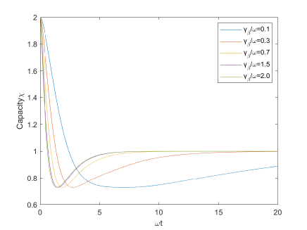
fig.1a

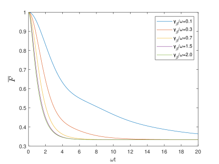
fig.1b

Figure 1: (Color online) The capacities $\chi$ of super-dense coding and the average fidelity $\overline{\mathcal{F}}$ of the teleportation of our system, under the influence of composite non-Markovian noise processes, when the dephasing noise coupling strength is fixed as $\Gamma_{\alpha}/\omega=1$, with various memory capacities $\gamma_{\beta}/\omega=0.1$,$0.3$,$0.7$,$1.5$,$2.0$, which in blue, red, yellow, purple and green colors, respectively.

To understand the degree of entanglement generation in non-Markovian relaxation process encounter with Markovian dephasing noise, we plot the capacities $\chi$ and average fidelity $\overline{\mathcal{F}}$ of our quantum system with the increase of inverse memory capacity $\gamma_{\beta}/\omega$ (from $0.1\sim 2.0$), in Fig.(1a)-(1b). When there is long system-environment memory ($\gamma_{\beta}/\omega=0.1$), the backflow of information into quantum systems delays the decoherence between the qubits, improves the $\chi$ and $\overline{\mathcal{F}}$. With the inverse memory time parameter $\gamma_{\beta}$ increases, decoherence gets faster, and less the $\chi$ and $\overline{\mathcal{F}}$. The higher capacities and fidelity rely on longer memory time ($1/\gamma_{\beta}$) shows robustness of non-Markovian composite noises on entanglement generation compare to the near Markovian or classical processes. Again, this proves the suggestion of Yu Ting et al. T.Yu(2004) ; Jing(2013) ; Jing(2015) ; Jing(2018) ; T.Yu(1999) ; YuTing2004 ; LuoS.L.(2010) , that with an increase in non-Markovian noise memory capacity, quantum systems become more tolerant toward decoherence induced by the environment; information from the environment flows back into the system itself and restores some of the coherence between the qubits.

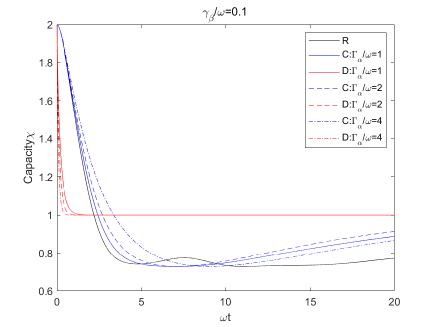
fig.2a

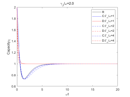
fig.2b

Figure 2: (Color online) Capacities $\chi$ of the two-level two-qubit quantum systems influenced by Markovian dephasing noise in a non-Markovian relaxation process, with various memory capacities; (a)$\gamma_{\beta}/\omega=0.1,$ (b)$\gamma_{\beta}/\omega=2.0$. The R, D, and C are the capacities $\chi$ under non-Markovian pure relaxation, Markovian pure dephasing, and composite non-Markovian noises, respectively. $\Gamma_{\beta}/\omega=1,2,4$ are fixed parameters presenting dephasing noise coupling strengths, drawn with solid, dashed, and dot-dashed lines.

The next step is to learn how Markovian dephasing noise contributes to information preservation, which introduced to quantum super-dense coding processes by a magnetic field, when non-Markovian relaxation occurs. We compare the differences of capacities $\chi$ of super-dense coding with the various noise types; the solid black curve labeled with R shows the pure relaxation processes, the red curves labeled with D show the Markovian dephasing noise processes, the blue curves labeled with C show the composite noise processes. The Fig.2(a,b) are organized as increase of $\gamma_{\beta}$, and in each figures the dephasing decoupling rates $\Gamma_{\alpha}/\omega$ are increased from 1~4. Fig.2a shows, when the systems under go strong non-Markovian processes with inverse memory capacity $\gamma_{\beta}/\omega=0.1$. All three groups of different colored curves with the same dephasing coupling strengths $\Gamma_{\alpha}$ can be divided in to two regions. In a moderate-time scale $0<\omega t<\tau$, with the value $2.5<\tau<3.5$, the systems under the mixture noises C have the higher capacities than the systems under pure dephasing D or relaxation R noises. The increasing $\Gamma_{\alpha}$ yield even higher capacities and longer delay of $\tau$. For the rest of the timescale $3.5<\omega t$, the capacities $\chi$ of system under mixture noises C is higher than that system under the pure relaxation noises most of the time, but lower than the pure dephasing processes D. When the system embedded in mixture noises environment, which are blue curves C, the capacities $\chi$ of the system enhanced comparatively with the increase of $\Gamma_{\alpha}$. Hence our noise control protocol for two-qubit systems works for canceling relaxation effects in dissipation processes.

When the relaxation noise is a near Markovian with $\gamma_{\beta}/\omega=2.0$ T.Yu(2004) ; Jing(2018) ; ZhaoXY(2011) , we obtain Fig.2b. Due to a smaller non-Markovian memory capacity $1/\gamma_{\beta}$, all three noise type scenarios show significantly faster decay compared to Fig.2a. Its hard to distinguish the pure relaxation R from mixture noises C at smaller dephasing decoupling rate $\Gamma_{\alpha}/\omega=1$, but the higher dephasing decoupling rates $\Gamma_{\alpha}/\omega=2,4$ benefit the mixture noise. By introducing a dephasing noise in the near Markovian relaxation noise, it improves capacities of mixture noises. However, under the high dephasing decoupling rate $\Gamma_{\alpha}/\omega=4$, the capacities $\chi$ of mixture noises are slightly higher than the system under the pure dephasing noise D in a very short time scale $0<\omega t<1.0$.

The Fig.2(a,b) show that, by introducing a dephasing noise into two-qubit non-Markovian relaxation processes, the decay of super-dense coding capacities $\chi$ can be delayed. The stronger dephasing noise coupling strength $\Gamma_{\alpha}$, i.e. strong magnetic field, delays the decay even noticeably. Adding the differences made by non-Markovian memory capacity $1/\gamma_{\beta}$ into consideration; with the help of high memory capacity $1/\gamma_{\beta}$ and strong dephasing noise coupling strength $\Gamma_{\alpha}$ significantly delay the decay of capacities $\chi$ of super-dense coding (in Fig2a blue dot-dash lines), than when they work separately. Thus, by inducing a strong dephasing noise into the non-Markovian relaxation processes, delay the decoherence and help the system to performs better on super-dense coding.

In order to study how the dephasing noise effects relaxation process on quantum teleportation, we obtain the average fidelity $\overline{\mathcal{F}}$ for these three types of noise scenarios with different inverse memory capacity $\gamma_{\beta}/\omega=0.1,2.0$, repectively in Fig.3(a,b). The Fig.3a shows the average fidelity dynamics driven by these three noise types; non-Markovian pure relaxation noise (black line R), non-Markovian composite noises (blue lines C) and Markovian dephasing noise (red lines D). Similar to above studies on capacities of super-dense coding, in Fig.3a the average fidelity of two-qubit system with a strong non-Markovian relaxation processes, when the memory capacity $\gamma_{\beta}/\omega=0.1$, all three different colored curves with the same dephasing coupling strength $\Gamma_{\alpha}$ can be divided in to three regions. In a moderate-time scale $0<\omega t<\tau_{1}$, with the value $3.5<\tau_{1}<5.5$, the system under the mixture noises have better average fidelity than the systems with pure relaxation R or pure dephasing D. The second region is $3.5<\omega t<\tau_{2}$, with $5.0<\tau_{2}<6.5$, that the average fidelity of mixture noises C are higher than the pure non-Markovian noise R, but smaller than the pure dephasing noise D. The third is in $6.5<\omega t$, that mixture noises C smaller than both other two noise types. As for the rest of the period, mixture noises C smaller than other two noise types for long-time scale. We can clearly see that among these three regions: the proposed noise control protocol works well to mitigate both pure Markovian dephasing noise process and pure non-Markovian relaxation process at the first region, and works only for pure non-Markovian relaxation not for dephasing noise. The average fidelity improves noticeably with the higher dephasing coupling strength $\Gamma_{\alpha}$, when there is strong dephasing coupling strength $\Gamma_{\alpha}/\omega=4$, result in way better average fidelity and more delay of the $\tau_{1}$ and $\tau_{2}$.

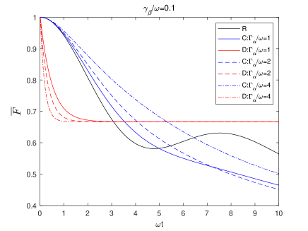
fig.3a

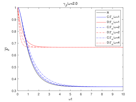
fig.3b

Figure 3: (Color online) Average fidelity $\overline{\mathcal{F}}$ of a two-qubit state influenced by Markovian dephasing noise in the non-Markovian relaxation process with various memory capacities: (a)$\gamma_{\beta}/\omega=0.1,$ (b)$\gamma_{\beta}/\omega=2.0$. R, C, and D correspond to the dynamics under pure non-Markovian relaxation, non-Markovian composite and pure dephasing processes, respectively. $\Gamma_{\beta}/\omega=1,2,4$ is a fixed parameter representing the dephasing noise coupling strengths, drawn with solid, dashed and dot-dashed lines.

When the inverse memory capacity increases to near Markovian $\gamma_{\beta}/\omega=2.0$ in Fig.3b, the average fidelity $\overline{\mathcal{F}}$ of teleportation for all these noise type scenarios decay significantly faster than in strong non-Markovian $\gamma_{\beta}/\omega=0.1$. The average fidelity $\overline{\mathcal{F}}$ dynamics evolves in the similar pattern as in Fig.3a, but at much faster rate, the values of $\tau_{1}$ and $\tau_{2}$ shortens significantly. Thus, indicate the fewer backflow of information makes differences between the Fig.3a and Fig.3b, as a property of a non-Markovian process.

The above works show that, the degeneration of open quantum systems are inevitable, but by inducing Markovian dephasing noise with the introducing magnetic field in the non-Markovian relaxation processes, the two-qubit systems have better average fidelity $\overline{\mathcal{F}}$ and super-dense coding capacities $\chi$, compare to the two-qubit systems with pure non-Markovian pure relaxation noise processes or pure dephasing processes in the moderate-time scale. Jing Jing(2018) showed that the average fidelity of single-qubit can be improved by mixing the dephasing noise with the non-Markovian relaxation noise processes, and he proposed a control principle: To mutually cancel two unwanted noisy processes enforced in the unitary evolution of the quantum system, the characteristic time scales of these two processes should be separable. In our studies on average fidelity $\overline{\mathcal{F}}$ of teleportation and capacity $\chi$ of super-dense coding in the two-qubit cases in (Fig.1,2,3), with the increase of non-Markovian memory capacites $1/\gamma_{\beta}$, more information backflow into quantum systems and strengthen the correlation between qubits by restoring the entanglement that lost in the environment. And with the increase the strecngth of magnetic field leads with high dephaing noise coupling strength $\Gamma_{\alpha}$ in non-Markovian composite noises process, it improves the efficiency of teleportation and quantum super-dense coding comparably than other two types of noise scenarios. Since our target is two-qubit quantum system, these noises are chosen to be enforced on qubits, simultaneously, and with equal strengths; thus, when measurements are performed, $\overline{\mathcal{F}}$ and $\chi$ are treated equally. This quantum noise control protocol does not need to perform measurements in the way of Zeno noise controlSudarshan(1997) (33), in fact just by apply a magnetic field, that introduce dephasing noise and increase its coupling strength, the quantum systems correlation increases, enhance super-dense coding capacity and fidelity of quantum teleportation compared to when there is only one types of noise cases.

IV conclusion

In this work, we studied the quantum teleportation and super-dense coding in the open two-qubit system under the non-Markovian approximation, and the environmental noises are chosen as three distinct types: Markovian pure dephasing noise, non-Markovian pure relaxation noise, and mixtures of these noises. For simplicity, these noises are from two separate baths. By comparing these three groups of results for average fidelity $\overline{\mathcal{F}}$ and capacity $\chi$, we found that by introducing strong magnetic field to induce dephasing noise as a noise control protocol on the two-qubit non-Markovian relaxation processes, we successfully enhanced the average fidelity $\overline{\mathcal{F}}$ of teleportation and capacity $\chi$ of super-dense coding in some time-scale. At the same time, by studying different strengths of non-Markovian memory time scales $1/\gamma_{\beta}$, we prove that when there is a strong non-Makovian process, decoherence delayed significantly and vice versa, which is proven by others on separate papers for different cases Chen(2014) ; Jing(2013) ; Jing(2015) ; Jing(2018) ; L.Di=0000F3si(1998) ; LuoS.L.(2010) ; T.Yu(1999) ; T.Yu(2004) ; YuTing2004 ; ZhaoXY(2011) . Our findings emphasize that, when two-qubit in an environment of combined semi-classical and non-Markovian noises, the two noises cancel each other out and suppressed the non-Markovian open quantum system early in the process, for that the extra magnetic is needed. The extra magnetic field helps to reduce the coupling strength $\widetilde{\Gamma}_{\beta}$ and increase the inverse memory capacity $\tilde{\gamma_{\beta}}$ of composite non-Markovian OU noise, the relation between these two parameters are need to be further study.

- (1) A. K. Ekert, Phys. Rev. Lett. 67,661 (1991).
- (2) C. H. Bennett, G. Brassard, C. Crépeau, R. Jozsa, A. Peres, and W. K. Wootters, Phys. Rev. Lett. 70, 1895 (1993).
- (3) C. H. Bennett, and S. J. Wiesner, Phys. Rev. Lett. 69, 2881 (1992).
- (4) M. A. Nielsen and I. L. Chuang, Quantum Computation and Quantum Information (Cambridge University Press, Cambridge, 2000).
- (5) P. W. Shor, Phys. Rev. A 52, R2493 (1995).
- (6) A. M. Steane, Phys. Rev. Lett. 77, 793 (1996b).
- (7) D. A. Lidar, I. L. Chuang, and K. B. Whaley, Phys. Rev. Lett. 81, 2594 (1998).
- (8) P. G. Kwiat et al., Science 290, 498 (2000).
- (9) L. Viola, E. Knill and S. Lloyd, Phys. Rev. Lett. 82, 2417 (1999).
- (10) X. X. Yi, and C. P. Sun, Phys. Lett. A 262, 287 (1999).
- (11) W. T. Strunz and T. Yu, Phys. Rev. A 69, 052115 (2004).
- (12) B. Corn and T. Yu, Quantum Inf. Process. 8,565 (2009).
- (13) J. Jing and L.-A.Wu, Sci. Rep. 3, 2746 (2013).
- (14) J. Jing, R. Li, J. Q. You, and T. Yu, Phys. Rev. A 91, 022109 (2015).
- (15) Beige A. Braun, D. Tregenna, B. Knight, Phys. Rev. Lett. 85, 1762 (2000).
- (16) Jun Jing, Y. Ting, Chi-Hang Lam, J. Q. You and Lian-Ao Wu, Phys. Rev. A 97,012104 (2018).
- (17) L. Diósi, N. Gisin, and W. T. Strunz, Phys.Rev.A 58,1699 (1998).
- (18) T. Yu, L. Diosi, N. Gisin and W. T. Strunz, Phys.Rev. A 60, 91 (1999).
- (19) Yusui Chen, J. Q. You and Ting Yu, Phys. Rev. A 90,052104 (2014).
- (20) A. S. Holevo, Probl. Inf. Transm. 9 177 (1973).
- (21) D. Boschi, S. Branca, F. De Martini, L. Hardy & S. Popescu, Phys. Rev. Lett. 80, 1121–1125 (1998).
- (22) I. Marcikic, H. de Riedmatten, W. Tittel, H. Zbinden and N. Gisin, Nature 421, 509–513 (2003).
- (23) Xiao-Song Ma et al.,Nature 489,269-273 (2012).
- (24) Dik Bouwmeester, Jian-Wei Pan, et al., Nature 390, 575–579 (1997).
- (25) R. Jozsa, J. Mod. Opt., 41 2315 (1994) .
- (26) E. Lombardi, F. Sciarrino, S. Popescu, et al. Phys. Rev. Lett. 88, 070402 (2002).
- (27) G. Bowen, S. Bose, Phys. Rev. Lett. 87, 267901 (2001).
- (28) Guo-Feng Zhang, Phys. Rev. A 75, 034304 (2007).
- (29) T. Yu, and J. H. Eberly, Phys. Rev. Lett. 93, 140404 (2004).
- (30) S. L. Luo, S. S. Fu, Phys. Rev. A 82, 034302 (2010).
- (31) Xinyu Zhao, Jun Jing, Brittany Corn, Ting Yu, Phys. Rev. A 84,032101 (2011).
- (32) L. Hughston, R. Jozsa, and W. Wootters, Phys. Lett. A 183, 14, (1993).
- (33) B. Misra, E. C. G. Sudarshan, Journal of Mathematical Physics, Vol.18(4):756-763 (1997).