Wrinkles, folds and ripplocations: unusual deformation structures of confined elastic sheets at non-zero temperatures

Abstract

We study the deformation of a fluctuating crystalline sheet confined between two flat rigid walls as a simple model for layered solids where bonds among atoms within the same layer are much stronger than those between layers. When subjected to sufficiently high loads in an appropriate geometry, these solids deform and fail in unconventional ways. Recent experiments suggest that configurations named ripplocations, where a layer folds backwards over itself, are involved. These structures are distinct and separated by large free energy barriers from smooth ripples of the atomic layers that are always present at any non-zero temperature. We use Monte Carlo simulation in combination with an umbrella sampling technique to obtain conditions under which such structures form and study their specific experimental signatures.

I Introduction

The current understanding of the mechanical response of materials to large external stress CL ; Landau ; rob is mostly based on ideas applicable to simple close-packed solids CL . Prevalent theories of irreversible deformation, therefore, invariably involve the nucleation and motion of lattice defects such as dislocations hirth ; nabarro . Recently, it has been observed that spatially confined flexible membranes deform by reorganizing their morphology to form hierarchical structures of great complexity hierarchy . Wrinkles, ripples, folds Milner ; Cerda-Maha ; Zhang ; Brau ; Li-wrinkle , as well as higher order structures like pleats sas4 ; sas7 are ubiquitous both in nature and in emergent technology. They have been observed in biological tissues spectrin1 ; spectrin2 , polymer sheets muthu , and many other low-dimensional materials involving flexible sheets and membranes origami ; kirigami1 ; kirigami2 ; irvine ; grason1 ; grason2 ; grason3 ; narayanan1 ; narayanan2 ; flat-fold1 ; flat-fold2 . Similar structures, named ripplocations, have been introduced to describe new kink-like deformation mechanisms  frank , associated with the buckling of surface layers in response to mechanical loading of van der Waals-layered solids such as MoS₂ or the MAX family of solids like Ti₃SiC₂, graphene etc. barsoum2003 ; 1barsoum2003 ; barsoum2004 ; 1barsoum2004 ; barsoum2005 ; barsoum2013 ; kushima2015 ; gruber2016 ; Tucker ; Freiburg . Ripplocations are structurally distinct from conventional dislocations in bulk crystals rob ; nabarro ; hirth . Such patterns are prevalent in many types of deformed layered materials spanning more than 13 orders of magnitude in scale Barsoum-Zhao , including massive geological formations such as phyllosilicates in the lithosphere Aslin2019 .

Small compressive strains in layered materials result in the formation of smooth undulations, known as ripples or wrinkles. These undulations are associated with a broad distribution of strain energy. At larger compression, the strain energy can be localized, leading to structures with sharp folds. Thus, there can be a wrinkle-to-fold transition with increasing compressive strain. At zero temperature, $T=0$, this behavior can be described by the Föppl-von Kármán equations Landau that in general cannot be solved analytically. Nevertheless, approximate theories of the wrinkle-to-fold instability have been derived Cerda-Maha . Further compression leads to higher-order deformation patterns where atomic layers glide relative to each other without breaking the in-plane bonds and producing a pleat (see Fig.1) or ripplocation. These structures involve large and singular deformations of flat sheets and are intractable within existing elasticity theory.

Although the $T=0$ energetics of system-spanning ripplocation has been studied Freiburg ; kushima2015 , many questions remain unanswered. A completely open issue is the mechanism for the formation of ripplocations at finite temperatures, $T\neq 0$. Also the following questions about the emergence of ripplocations are not well understood: What are the microscopic precursors and intermediate states that give rise to these higher order structures? How are such incipient structures to be distinguished from thermally driven random height fluctuations? What is the typical free energy barrier involved in their formation? What are the typical mechanical signatures of ripplocation formation?

In this paper, we address these issues in the context of a thin fluctuating sheet modeled as a network of connected vertices ordered in a triangular lattice and confined between two rigid layers. Our model system does not correspond to any particular material. Rather, we provide answers to some of the many questions raised above depending on physical parameters such as the temperature, the stiffness of the layers, the intra-layer mechanical coupling etc., which vary from material to material. Our calculations explicitly take into account the effect of finite temperature $T>0$ and therefore represent a definite advance on earlier work. We show that ripplocation like structures, which are the generalization of the purely two-dimensional (2D) pleats studied earlier sas4 ; sas7 , readily form following a phase transition from an essentially flat sheet containing at most thermally generated ripples. These phases co-exist at a first-order boundary. The free energy barrier between these phases at co-existence is large but reduces as the solid is deformed. For certain choices of parameters the ripplocated phase remains metastable at all values of strain.

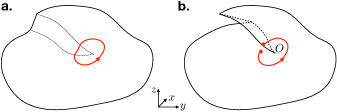
Figure 1: Schematic figure showing a ripple a. and a ripplocation b. in a layered solid. The red circles around the point $O$ with arrows show Burgers circuits on the layer. In a ripple, such a circuit returns to the same point on the layer whereas if a ripplocation is present, the circuit returns to a point displaced in the direction perpendicular to the layer. Assuming that the boundary of the sheet is single valued, every point, $O$, for a ripplocation is associated with a corresponding point $O^{\prime}$ (not shown for clarity) where an identical circuit produces an equal displacement of opposite sign.

The difference between normal, smooth fluctuations of the height of a sheet, which has been variously called a wrinkle, ripple or fold, and one that comprises a pleat or ripplocation is explained schematically in Fig.1. A smooth wrinkle (c.f. Fig.1a), is always representable as a single valued function $z(x,y)$. Traveling along any closed loop on the surface always ends in a return to the starting point anywhere on this surface. The scale of these smooth ripples may vary. We denote small random fluctuations of height as wrinkles and large collective height fluctuations are called folds.

In contrast, a ripplocation or pleat (see Fig.1b) involves a multivalued height function $z(x,y)$ and there is the existence of points $O$ for which closed loops enclosing them are finally always displaced by an amount $\Delta z$ from the starting point perpendicular to the plane. Now imagine a pair of such singular points $O$ and $O^{\prime}$ adjacent to one another with displacements $\pm\Delta z$, of opposite signs. These can be viewed as the analogs of a dislocation dipole in a 2D solid CL ; rob . However, in dislocation dipoles, the displacement, known as the Burgers vector, is within the plane and along the line joining $O$ and $O^{\prime}$. We show later that system spanning ripplocations form when $O$ and $O^{\prime}$ separate in the presence of external loads.

In order to study the statistical mechanics of ripplocations, we need to construct an appropriate collective variable to be used as a reaction co-ordinate in order to obtain the free energy surface as well as free energy barriers. To this end, we employ a quantity for the measure of non-affine displacements that was first introduced in the study of mechanical deformations in glasses falk . Subsequently, this quantity has been generalized sas1 and used to investigate defects in crystals popli , pleats in permanently bonded networks sas4 ; sas7 , the origin of rigidity of crystalline solids pnas , and biologically important conformation changes in proteins protein .

The rest of the paper is organized as follows. In the next section (Section II), we introduce our model for the fluctuating, confined two-dimensional sheet, define the collective variable to measure non-affine displacements and give the details of our simulation method. In Section III, we discuss our results starting with a re-examination of the ripple-to-fold instability in our model, followed by a description of the equilibrium transition from ripple to ripplocation at non-zero temperatures and the presentation of the computed equilibrium phase diagram. Then, intermediate structures that arise during nucleation of the ripplocated phase are analyzed. Finally, we conclude the paper in Section IV by discussing the possible experimental implications and future directions of research.

II Model and Methods

II.1 The fluctuating sheet as a model network

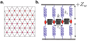
Figure 2: Schematic of the model network confined by two rigid walls. a. Top view showing the initial triangular lattice in the $xy$ plane. The red colored beads indicate the initial positions of the particles. b. Lateral view showing the springs (blue) connecting the particles with the confining walls.

We model the fluctuating sheet as a network of vertices connected by elastic bonds. The model consists of $N$ particles, interacting via a harmonic potential with respect to a 2D reference network structure (see below) and a repulsive Weeks-Chandler-Andersen (WCA) CL potential $u_{\rm WCA}(r)$. The latter potential is defined by

$$u_{\rm WCA}(r) = \begin{cases}4e\left[\left(\frac{\sigma_{0}}{r}\right)^{12}-\left(\frac{\sigma_{0}}{r}\right)^{6}\right]+e&\text{if }|r|\leq r_{c}\\ 0&\text{otherwise},\end{cases}$$ (1)

with $r$ the distance between a pair of particles. The radius $r_{c}$ is set to $r_{c}=2^{1/6}\sigma_{0}$. So the potential, defined by Eq. (1), is a Lennard-Jones potential that is cut off and shifted to zero at its minimum.

The initial positions of the network are at ${{\bf R}_{i}}$ ($i=1,\ldots,N$), corresponding to an ideal triangular reference lattice in the $xy$ plane (Fig.2a). The particles are connected by harmonic bonds of stiffness $k$ and length $R_{0}=|{\bf R}_{i}-{\bf R}_{j}|$ (with ${\bf R}_{i}$ and ${\bf R}_{j}$ being reference lattice vectors of two adjacent particles $i$ and $j$, respectively). In $z$ direction, the network is confined by two parallel walls that are at a distance $\pm Z_{w}$ on either side of the triangular lattice plane. So the Hamiltonian of the harmonic network model is given by

$$\mathcal{H}=\mathcal{H}_{0}+\mathcal{H}_{\rm WCA}+\mathcal{H}^{\rm wall}$$ (2)

Here, $\mathcal{H}_{0}$ consists of the kinetic energy and the potential energy due to the harmonic bonds,

$$\mathcal{H}_{0}=\sum_{i=1}^{N}\frac{{\bf p}_{i}^{2}}{2m}+\frac{k}{2}\sum_{i=1}^{N}\sum_{j\in\Omega,j<i}(|{\bf r}_{j}-{\bf r}_{i}|-|{\bf R}_{j}-{\bf R}_{i}|)^{2}$$ (3)

with $m$ the mass of a particle, ${\bf p}_{i}$ the momentum of particle $i$, and ${\bf r}_{i}$ its instantaneous position. $\Omega$ signifies the interaction volume, which for each node $i$ comprises all its nearest neighbours $j$ on the triangular lattice. The term $\mathcal{H}_{\rm WCA}$ in Eq. (2) is the potential energy due to the repulsive WCA interactions,

$$\mathcal{H}_{\rm WCA}=\sum_{i=1}^{N}\sum_{j>i}u_{\rm WCA}(r_{ij}),$$ (4)

where $r_{ij}=|{\bf r}_{j}-{\bf r}_{j}|$ and $\sum_{i=1}^{N}\sum_{j>i}$ denotes the double sum over all $\frac{1}{2}N(N-1)$ particle pairs.

The term $\mathcal{H}^{\rm wall}$ describes the interaction of the particles with the confining flat walls. The particles are connected in $z$ direction to both the walls by harmonic springs of unstretched length $Z_{o}$ and stiffness $k_{z}$. In addition, there are repulsive WCA interactions between the particles and the walls in $z$ direction. Thus, the particle-wall interactions are given by

$$\mathcal{H}^{\rm wall} = \mathcal{H}^{\rm wall}_{0}+\mathcal{H}^{\rm wall}_{\rm WCA}$$

$$\mathcal{H}^{\rm wall}_{0} = \sum_{i}\frac{k_{z}}{2}\left\{(|Z_{i}-Z_{w}|-Z_{0})^{2}\right.$$

$$\left.+(|Z_{i}+Z_{w}|-Z_{0})^{2}\right\}$$

$$\mathcal{H}^{\rm wall}_{\rm WCA} = \sum_{i}[u_{\rm WCA}^{\rm w}(Z_{w}-Z_{i})+u_{\rm WCA}^{\rm w}(Z_{i}+Z_{w})]$$

$$u_{\rm WCA}^{\rm w}(r) = \begin{cases}4e_{\rm w}\left[\left(\frac{\sigma_{\rm w}}{r}\right)^{12}-\left(\frac{\sigma_{\rm w}}{r}\right)^{6}\right]+e_{\rm w}&\text{if}~{}|r|\leq Z_{c}\\ 0&\text{otherwise}\end{cases}$$

with $Z_{c}=2^{1/6}\sigma_{\rm w}$. That the particles cannot overlap with each other or with the walls is ensured by finite values of $\sigma_{0}$ and $\sigma_{\rm w}$. We chose the unit of length as $R_{0}$ and the unit of energy as $e$. For large values of $\sigma_{0}(\simeq R_{0})$, slip dislocations can occur on application of compression. These are not of interest here so we present results for $\sigma_{0}=0.1R_{0}$ and $e=1.0$. The qualitative results seem to be largely insensitive to the value of $\sigma_{0}$ as long as $\sigma_{0}\ll R_{0}$. For our calculations, we choose $Z_{0}=2.4,R_{0}=1.0$ so that the ratio $Z_{0}/R_{0}$ is similar to the ratio of the typical in-plane interparticle distance to the distance between layers in a solid such as graphite CL . We have set the parameters $m=1$,$k=1$,$\sigma_{\rm w}=\sigma_{0}$ and $e_{\rm w}=e$.

II.2 The collective order parameter for ripplocations

The primary ingredient for our analysis is contained in a paper by Ganguly et al. sas1 , which shows that any displacement of atoms away from a reference position can be classified into two mutually orthogonal subspaces using a projection operator ${\mathsf{P}}(\{{\bf R}\})$ which depends only on the set of lattice vectors $\{{\bf R}\}$ defining a suitably chosen reference configuration. These subspaces may be classified as “affine” and “non-affine” depending on whether or not the instantaneous particle positions, $\{{\bf r}\}$, of the displaced structures can be represented as an affine deformation (homogeneous strain) of the reference configuration. The affine subspace may be parameterized by the local deformation tensor ${\mathsf{D}}$ while the non-affine part of the displacements is parameterized by a local scalar $\chi$. The latter is the least square error made by fitting $\{{\bf r}\}$ to a “best fit” ${\mathsf{D}}$. Various thermodynamic quantities such as the ensemble average $\langle\chi\rangle$ and the spatio-temporal correlation functions $\langle\chi(0,0)\chi({\bf R},t)\rangle$ can be obtained analytically sas1 ; sas2 . The spatial average $X=N^{-1}\sum_{i}\chi({\bf R}_{i})$ behaves as a thermodynamic variable with a conjugate field $h_{X}$ sas2 .

We study the network in the presence of both $h_{X}$ and an externally imposed strain $\epsilon_{d}$. Specifically, we have a rectangular box whose dimensions are commensurate with the triangular lattice. The strain is implemented by expanding the simulation box along the $y$-direction and compressing it along the $x$- and $z$-direction by the same fractional amount $\epsilon_{d}$ while conserving volume to linear order. Tuning $h_{X}$ can either suppress or enhance lattice defects and this can be used to study the deformation of solids. Indeed, we have shown pnas that an initially ideal (defect-free) 2D crystal when deformed becomes metastable for infinitesimal deformation and tends to decay into the stable state where stress is eliminated by slipping of crystalline planes (lines in 2D). This is the dynamical consequence of an underlying first-order phase transition as a function of both $h_{X}$ and deformation. Although it is difficult (though not entirely impossible, see poplitrap ) to realize $h_{X}$ experimentally, this expansion of parameter space provides many physical insights, with experimentally realizable consequences being recovered in the $h_{X}\to 0$ limit. We therefore follow a strategy similar to that employed in Refs. sas4 ; sas7 ; pnas .

II.3 Successive umbrella sampling

To study the ripple-to-ripplocation transition as a function of $h_{X}$ and deformation at non-zero temperatures, an efficient computational scheme that is able to access structures with ripplocations starting from a flat sheet is required. While ripples are always present at non-zero temperatures, we show later that transition probabilities between ripples and ripplocations are exponentially small due to large barriers. One method that produces satisfactory results in this case is successive umbrella sampling Monte Carlo (SUS-MC) SUS , which has been used previously to study pleats in strictly two dimensional networks sas4 ; sas7 .

To implement SUS-MC for our system, we divide the range of the reaction coordinate $X$ into small windows and sample configurations generated by Metropolis Monte Carlo  binder ; ums in each window, keeping the system restricted to the chosen window for a predefined number of MC cycles. Beginning with $X=0$, histograms are recorded to keep track of accepted MC moves and how often the system tries to leave a window via its left or right boundary. The probability distribution $P(X)$ can then be computed from these histograms. Further details of the procedure can be found in our earlier work sas4 ; sas7 ; pnas . The computational effort needed for implementation of SUS-MC is nonetheless substantial and grows with $N$. This restricts the system size. By studying the finite size effects at $T>0$, conclusions can be drawn by extrapolating to the thermodynamic limit $N\to\infty$. In this work, we present results mostly for $N=900$ vertices, mentioning consequences of finite size later wherever appropriate. We used $\beta=1/(k_{\rm B}T)=200$ throughout; results at other temperatures are qualitatively similar. We divide the range $0<X<0.4$ into $800$ windows to obtain sufficient resolution. For sufficiently averaged $P(X)$ values, $2\times 10^{8}$ trial moves are required in each window. Once we obtain $P(X)$ for one particular combination of $h_{X}$ and $\epsilon_{d}$ value, we use the histogram reweighting technique to determine $P(X)$ at any other $h_{X}$ borgs90 ; ferrenberg88 .

III Wrinkle, fold and ripplocation transitions

When a flexible sheet is compressed, at $T=0$, two specific kinds of transitions are observed. Firstly, small undulations, or wrinkles appear, which on further compression give rise to folds Milner ; Cerda-Maha ; Zhang ; Brau ; Li-wrinkle . As explained in the Introduction, the height variable in both wrinkles and folds is single-valued and we collectively call these configurations ripples. Under certain circumstances, such rippled phases can produce multi-valued height fluctuations, which we will refer to as ripplocations or pleats. We describe below first the wrinkle to fold transition at $T>0$, and then consider and analyze the transition to the ripplocated phase.

III.1 Finite temperature wrinkle to fold instability

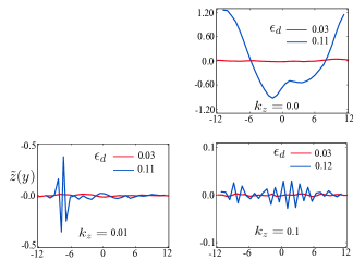
Figure 3: a. Plot of $\langle\Delta\rangle$ vs. $\epsilon_{d}$ at $R_{1}$ (see text) obtained from SUS-MC of a $30\times 30$ lattice with $k_{z}=0.0,0.01,0.1$. The inset shows the definition of the length scale $\Lambda$. Note that $\langle\Delta\rangle$ undergoes a finite jump at $\epsilon_{d}\approx 0.08$ for $k_{z}=0.0$ and at $\epsilon_{d}\approx 0.1$ at $k_{z}=0.01$ signifying a wrinkle-to-fold transition. Note that for $k_{z}=0.1$, such a transition is not observed. The green and blue circles indicate the $\epsilon_{d}$ at the ripple-ripplocation transition for $k_{z}=0.01$ and $k_{z}=0.1$, respectively.The $x$-averaged $z$-value $\tilde{z}(y)$ at each $y$ is plotted before and after the wrinkle-fold transition for b. $k_{z}=0.0$ and c. $k_{z}=0.01$ d. Plot of $\tilde{z}(y)$ vs. $y$ for $k_{z}=0.1$ and $\epsilon_{d}=0.03,0.12$.

The elastic instability that gives rise to the wrinkle-to-fold transition persists at $T>0$. However, due to the thermal motion at $T>0$, it becomes difficult to distinguish between thermal height fluctuations and elastic buckling. Nevertheless, we define the quantity $\Delta={\rm max}[|\tilde{z}(y)|]/\Lambda$, where $\tilde{z}(y)$ is the $x$-averaged value of the height $z$ at each position $y$ along the direction of compression. We define $\Lambda$ as a typical width of height fluctuations (see Fig.3, inset). We calculate the thermal and spatial average $\langle\Delta\rangle$ from configurations obtained from our SUS-MC simulations. We ensure that these configurations contain only the ripple phase, i.e. the height function is always single-valued on average. In the next section (Section III.2) we show that the probability distribution $P(X)$ always has a maximum (or the effective dimensionless free energy $-\ln P(X)$ a minimum) at small $X$ (denoted by $R_{1}$), which corresponds to the ripple phase. Here, we analyze configurations that belong to this small $X$-minimum as extracted from our SUS-MC calculations.

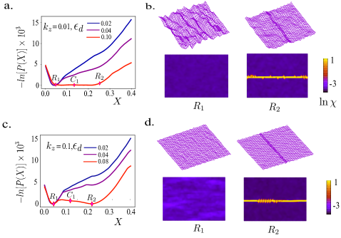
Figure 4: a. Plot of effective free energy $-\ln(P(X))$ obtained from SUS-MC of a $30\times 30$ network with $k_{z}=0.01$ for ${\epsilon}_{d}=0.02,0.04,0.10$. b. Configurations at $R_{1}$, $R_{2}$ for $k_{z}=0.01$. c. Same as (a.) for $k_{z}=0.1$ for ${\epsilon}_{d}=0.02,0.04,0.08$. d. Configurations for $k_{z}=0.1$ at $R_{1}$, $R_{2}$. In each case, the first minimum is a ripple, and the second corresponds to a configuration with a ripplocation. In b. and d. the upper panel is the averaged 3D configuration of the lattice and the lower panel shows the 2D projections colored according to local $\chi$ values in the $xy$ plane.

Figure 3a shows the $\langle\Delta\rangle$ vs. $\epsilon_{d}$ graph for different values of confinement. The value of $\langle\Delta\rangle$ shows a finite jump for $k_{z}=0.0,0.01$ at $\epsilon_{d}=\epsilon_{w\to f}$ signifying the well-known “wrinkle-to-fold transition”. For $k_{z}=0.0$ (see Fig.3 b) and at a strain value $\epsilon_{d}=0.03$ below $\epsilon_{w\to f}=0.08$, the network is characterized by small $z$-fluctuations from wrinkles. For $\epsilon_{d}>\epsilon_{w\to f}$, large amplitude folds are visible. Upon increasing confinement with $k_{z}=0.01$, (Fig.3 c) we observe that although single, sharp, small wavelength peaks indicating folds are prevalent at large strains $\epsilon_{d}>\epsilon_{w\to f}\approx 0.1$, the amplitudes of these folds are smaller in comparison to those at $k_{z}=0.0$. Note that even for very large strains, folds remain single-valued in the $z$-direction, and the value of $X$ remains small. For strong confinement, $k_{z}=0.1$, a wrinkle-to-fold transition is not observed (Fig 3 d): large folds remain suppressed even at large $\epsilon_{d}$.

III.2 Equilibrium ripple-to-ripplocation transition

In this section, we describe the equilibrium thermodynamic phase transition between the single-valued rippled phases and the multi-valued ripplocated phase of the fluctuating confined sheet at nonzero temperature.

In Fig.4 a, we show $-\ln(P(X))$ for a $30\times 30$ network and $3$ different values of ${\epsilon}_{d}$ keeping $h_{X}=0.0$. Here, we choose $k_{z}=0.01$. The qualitative features in each of the $3$ cases are similar. The first minimum $R_{1}$ at small $X$ corresponds to the ripple state. The ripplocation phase $R_{2}$ has a large value of $X$. From Fig.4 b it is evident that the region around the pleat has large local $\chi$ values. For larger values of $X$, there exist higher order patterns corresponding to a sheet with multiple ripplocations. Here, we concentrate only on the transition from a ripple state to one with a single ripplocation. On increasing the external strain, the barrier height between the two minima of the dimensionless free energy, $-\ln(P(X))$, decreases. For $\epsilon_{d}=0.10$, where the system is very close to the phase boundary, the barrier height is about $\sim 10~{}k_{\rm B}T$. Figure 4c shows $-\ln(P(C))$ for a network with $k_{z}=0.1$. The free energy at three different values of ${\epsilon}_{d}=0.02$, 0.04, 0.08 and at $h_{X}=0$ is qualitatively similar to the $k_{z}=0.01$ case. As before, the two minima at $R_{1}$ and $R_{2}$ represent the ripple and ripplocation phases, respectively. However, coexistence is achieved at a smaller $\epsilon\sim 0.08$. The barrier height near coexistence $\sim 80~{}k_{\rm B}T$ is significantly higher compared to that at $k_{z}=0.01$.

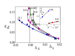
Figure 5: Phase diagram of a $30\times 30$ network in the $h_{X}$-$\epsilon_{d}$ plane showing the evolution of the boundary between the rippled and ripplocated phases as the strength of confinement $k_{z}$ is varied. The numbers above the curves indicate the corresponding value for $k_{z}$. .Note that as $k_{z}$ is reduced, the ripplocated phase ceases to exist at $h_{X}=0$ for any strain. The inset shows the coexistence point $\epsilon_{d}=\epsilon_{d}^{\rm coex}$ vs. $N^{-1}$ at $h_{X}=0$ for different values of $k_{z}$ as obtained from SUS-MC simulations. The value of $\epsilon_{d}^{\rm coex}$ decreases gradually as we approach $N\to\infty$.

The results for the equilibrium transition can be summarized in the phase diagram of Fig.5, where we have shown the equilibrium phase boundaries for a $N=30\times 30$ system at non-zero temperature for different confinement strengths $k_{z}$. With increasing confinement $k_{z}$, the ripplocated phase at $h_{X}$ is achieved at a smaller value of $\epsilon_{d}$. At the same time, as $k_{z}$ is reduced, we see that the $\epsilon_{d}$ vs. $h_{X}$ curve fails to intersect the $h_{X}=0$ line, indicating that the ripplocated phase ceases to exist at any strain for this case. Increasing $N$ shifts the phase diagram downwards to smaller values of $\epsilon_{d}$, and one obtains ripplocated phases at $h_{X}=0$ where none existed at smaller sizes. In the inset of Fig.5, we show that as $N\to\infty$, the ripplocated phases appears even without confinement. Note that the value of $\epsilon_{d}=\epsilon_{d}^{\rm coex}$ at $h_{X}=0$ decreases as one approaches $N\to\infty$. Similarly, the free energy barrier between the phases also has strong finite size effects.

It is clear from Fig.5a. that ripplocations either form at fixed $\epsilon_{d}$ by changing $h_{X}$ or at fixed $h_{X}$ by increasing $\epsilon_{d}$. The latter protocol is analogous to the standard yielding transition of solids at constant strain rate pnas ; sas7 .

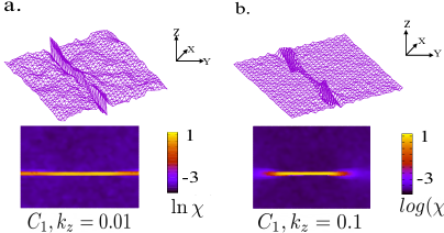
Figure 6: Configurations at intermediate region $C_{1}$ for a $30\times 30$ network obtained from SUS-MC sampling for a. $k_{z}=0.01$ (corresponding to Fig. 4a.) and b. $k_{z}=0.1$ (corresponding to Fig.4c). The upper panels show the averaged 3D configuration of the lattice and the lower panel the local $\chi$ maps.

III.3 Ripplocation precursors and intermediate structures

An advantage of our SUS-MC sampling method is apparent from Fig.6, where apart from the coexisting structures at the two minima, we are also able to discover the intermediate configurations along the transition path defined by the reaction coordinate $X$. This is the least free energy equilibrium path connecting the two phases. In Fig.6 a the intermediate structure corresponding to $C_{1}$ (Fig.4 a) is shown. The ripplocation in this case is preceded by the formation of a system-spanning fold. This is in sharp contrast with the formation of pleats in 2D sas7 , where the pleat forms by a local transformation that produces a “lip” with two tips where the displacement becomes singular.

The intermediate structure in Fig.6 b at $C_{1}$ (see Fig.4 c), on the other hand, reveals that in this case indeed the ripplocation is established by a local “pinching” where a lip with two tips is formed (cf. the point $O$ in Fig.1b). This pinching also results in the formation of a small bulge just near the tip. The lip then extends all around the periodic boundary and finally annihilates with itself once the ripplocation percolates throughout the sheet. This similarity with pleat formation in a flat 2D network can be explained by noting that with increasing confinement strength $k_{z}$, formation of a bulk system-spanning fold has a large energy cost; hence the network tends to remain mostly in the 2D plane.

The presence or absence of a preceding wrinkle-to-fold transition determines the intermediate configurations associated with the ripple-to-ripplocation transition. This is illustrated in Fig.3a. For systems with strong confinement above a certain threshold, where the wrinkle-to-fold transition is suppressed, formation of bulk system-spanning folds is prohibited (blue dot in Fig.3a); the pleat formation is preceded by local pinching. Below that threshold, system spanning folds are the precursors to ripplocation formation (green dot in Fig.3a). The free energy barrier between a ripple and a ripplocation is higher if an intermediate system spanning fold does not exist.

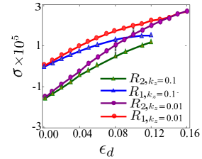
Figure 7: Stress vs. strain curves for rippled and ripplocated phases of a $30\times 30$ network. The nucleation of a ripplocated phase is always accompanied by a jump in stress (vertical dotted lines) as long as the strain is applied sufficiently slowly.

III.4 Mechanical signatures of the ripple-to-ripplocation transition

As mentioned earlier, ripples and ripplocations are separated by high barriers. Signatures of such high barrier values are apparent when we compute the stress for the ripple ($R_{1}$) and ripplocation ($R_{2}$) phases. This is illustrated in Fig.7, where we have plotted curves of conjugate stress $\sigma$ vs. $\epsilon_{d}$ for ripples and ripplocated phases at two different values of $k_{z}$ as obtained from SUS-MC calculations. We obtain $\sigma$ in the standard way ums by averaging the corresponding virial over a slab of thickness $Z_{w}$ centered about the plane $z=0$ wholly containing the reference lattice points. Since the value of $\sigma$ is computed for a possibly metastable phase, the rate of deformation $\dot{\epsilon}$ plays an important role.

For large $\dot{\epsilon}$ the transition happens at the limit of metastability of the rippled (wrinkled or folded) phase. For quasistatic deformation, on the other hand, the transition occurs at the equilibrium phase boundary. At any intermediate deformation rate, the transition should occur somewhere in between these limits. The ripplocation phase, which localizes stress within the ripplocation while relieving it elsewhere sas7 has a relatively lower value of average stress. The formation of the ripplocated phase is therefore always expected to be associated with a jump in the value of stress.

The formation of ripplocation is an irreversible deformation; once the network attains a ripplocation state it is unable to revert out of this due to high barriers. The jump in stress at the transition follows the barrier height between two phases; as we increase the confinement $k_{z}$, the magnitude of the jump in stress increases. This offers a unique way of distinguishing the formation of ripplocations from either system spanning folds or localized wrinkles in realistic systems by subjecting them to deformation experiments. Depending on whether a large or small jump is seen when structures are deformed at equal rates, one should be able to extract the barriers and estimate the magnitude of the confining interlayer potential. Small barriers point to a transition from a fold to a ripplocation while large barriers are associated with the formation of ripplocations directly from wrinkles. The deformation behavior of these materials is therefore highly non-linear barsoum2003 ; 1barsoum2003 ; barsoum2004 ; 1barsoum2004 ; barsoum2005 ; barsoum2013 ; kushima2015 ; gruber2016 ; Tucker ; Freiburg .

Unravelling the dynamics of this transition and predicting the yield point, i.e. the deformation at which the stress decreases, which is necessarily a function of the strain rate, requires more intense study; work in this direction is planned for the near future pnas ; reddy .

IV Summary and outlook

In this paper, we have described in detail the $T>0$ pleating transition and formation of a ripplocation in a confined 2D sheet with out-of-plane fluctuations when deformed by a pure shear. Our motivation is to understand how plastic deformation occurs in a system where defects or atomic rearrangements are not possible. Similar to our work on a “ghost network” sas4 ; sas7 , we show the existence of the ripple-to-ripplocation transition when such a sheet is confined by parallel walls but fluctuations in the perpendicular direction are allowed. The ripple phase evolves from wrinkles characterized by small height fluctuations at small strain to large amplitude folds at high strain values. While such wrinkle-to-fold transitions have been reported for a variety of situations in 2D membrane networks, ripplocations are a novel type of structure not identified in any of these earlier works Milner ; Cerda-Maha ; Zhang ; Brau ; Li-wrinkle where the surface is taken to be always single-valued. Establishing the existence of such multi-valued deformation structures as a consequence of a first-order pleating phase transition is a primary contribution of our work. In order to describe the transition we define an external field conjugate to the non-affine displacements $X$.The thermodynamic variable $X$ behaves as a reaction coordinate to describe our ripple-to-ripplocation transition.

The main conclusions of this work can be summarized as follows:

1. The response to deformation in our model is characterized by a first-order phase transition. The ripple phase and the ripplocation phase are separated by large free energy barriers. The free energy barrier between ripple and ripplocation strongly depends on the strength of the confinement.

2. Apart from this pleating transition, the wrinkle-to-fold transition is also present in our model. This transition influences the intermediate structures in the ripple-to-ripplocation transition.

3. The ripple to ripplocation transition occurs at smaller strains for higher values of confinement.

4. Two different types of ripplocation formation can be seen in our calculations, depending on the strength of the confinement. For weak confinement, the ripplocation is preceded by bulk system-spanning ripples. In case of stronger confinement, a pleat tip is formed, which percolates through the system to form ripplocations.

Finally, a word of caution. It should be pointed out that throughout this work, we distinguish between the terms ripple and ripplocation, depending on whether the height variable is single- or multi-valued, respectively. This may be contrasted with the term ”ripplocation” used in recent literature kushima2015 ; gruber2016 , which referred to any large localized variation of height.

Our model for a confined crystalline sheet could be modified in many ways, such that it becomes more realistic. Real confined membranes, e.g., do have an intrinsic curvatures and bending rigidity. This is also true for real layered solids. Such effects have been neglected in our conceptual model. However, regardless of the minute details, we believe that essential qualitative aspects of the pleating transition like the stress-strain curve, the finite-size effects and the intermediate structures will be similar to those described in this paper. We are in the process of extending our work to a realistic model of graphene where some of these questions can be addressed and the effect of ripplocation deformation on physical properties can be explored  sandhya .

The exact nature of the phases is also strongly dependent on the dynamics of external loading. Dynamical effects have been neglected in the present work and their incorporation will be an interesting exercise once accurate experimental results are available for comparison.

- (1) P. Chaikin and T. Lubensky, Principles of Condensed Matter Physics (Cambridge University Press, Cambridge, 1995).
- (2) L. Landau and E. M. Lifshitz, Theory of Elasticity, 3rd ed. (Pergamon, New York, 1986).
- (3) R. Phillips, Crystals, defects and microstructures: Modeling across scales (Cambridge University Press, Cambridge, 2004).
- (4) J. P. Hirth and J. Lothe, Theory of Dislocations (McGraw-Hill, New York, 1967).
- (5) F. R. N. Nabarro and M. S. Duesbery, Eds., Dislocations in Solids, Vol. 10 (Elsevier, Amsterdam, 1996), p.505-594.
- (6) H. Vandeparre, M. Pineirua, F. Brau, B. Roman, J. Bico, C. Gay, W. Bao, C. N. Lau, P. M. Reis, and P. Damman, Phys. Rev. Lett. 106, 224301 (2011).
- (7) S. T. Milner, J.-F. Joanny, and P. Pincus, Europhys. Lett. 9, 495 (1989).
- (8) E. Cerda and L. Mahadevan, Phys. Rev. Lett. 90, 074302 (2003).
- (9) Q. Zhang and T. A. Witten, Phys. Rev. E 76, 041608 (2007).
- (10) F. Brau, H. Vandeparre, A. Sabbah, C. Poulard, A. Boudaoud, and P. Damman, Nat. Phys. 7, 56 (2011).
- (11) B. Li, Y.-P. Cao, X.-Q. Feng, and H. Gao, Soft Matter 8, 5728 (2012).
- (12) S. Ganguly, P. Nath, J. Horbach, P. Sollich, S. Karmakar, and S. Sengupta, J. Chem. Phys. 146, 124501 (2017).
- (13) S. Ganguly, D. Das, J. Horbach, P. Sollich, S. Karmakar, and S. Sengupta, J. Chem. Phys. 149, 184503 (2018).
- (14) D. H. Boal, U. Seifert, and A. Zilker, Phys. Rev. Lett. 69, 3405 (1992).
- (15) H. Li and G. Lykotrafitis, Biophys. J. 102, 75 (2012).
- (16) M. Muthukumar, C. K. Ober, and E. L. Thomas, Science 277, 1225 (1997).
- (17) L. Mahadevan and S. Rica, Science 307, 1740 (2005).
- (18) D. M. Sussman, Y. Cho, T. Castle, X. Gong, E. Jung, S. Yang, and R. D. Kamien, Proc. Natl. Acad. Sci. USA 112, 7449 (2015).
- (19) T. Castle,Y. Cho, X. Gong, E. Jung, D. M. Sussman, S. Yang, and R. D. Kamien, Phys. Rev. Lett. 113, 245502 (2014).
- (20) W. T. M. Irvine, V. Vitelli, and P. M. Chaikin, Nature 468, 947 (2010).
- (21) G. M. Grason and B. Davidovitch, Proc. Natl. Acad. Sci. USA 110, 12893 (2013).
- (22) A. Azadi and G. M. Grason, Phys. Rev. Lett. 112, 225502 (2014).
- (23) A. Azadi and G. M. Grason, Phys. Rev. E 94, 013003 (2016).
- (24) H. King, R. D. Schroll, B. Davidovitch, and N. Menon, Proc. Natl. Acad. Sci. USA 109, 9716 (2012).
- (25) A. D. Cambou and N. Menon, Proc. Natl. Acad. Sci. USA 108, 14741 (2011).
- (26) L. H. Dudte, E. Vouga, T. Tachi, and L. Mahadevan, Nat. Mater. 15, 583 (2016).
- (27) J. L. Silverberg, J-H. Na, A. A. Evans, B. Liu, T. C. Hull, C. D. Santangelo, R. J. Lang, R. C. Hayward, and I. Cohen, Nat. Mater. 14, 389 (2015).
- (28) F. C. Frank and A. N. Stroh, Proc. Phys. Soc. London 65, 811 (1952).
- (29) M. W. Barsoum, T. Zhen, S. R. Kalidindi, M. Radovic, and A. Murugaiah, Nat. Mater. 2, 107 (2003).
- (30) A. Murugaiah, M. W. Barsoum, S. R. Kalidindi, and T. Zhen, J. Mater. Res. 19, 1139 (2004).
- (31) M. W. Barsoum, A. Murugaiah, S. R. Kalidindi, and T. Zhen, Phys. Rev. Lett. 92, 255508 (2004).
- (32) M. W. Barsoum, A. Murugaiah, S. R. Kalidindi, T. Zhen, and Y. Gogotsi, Carbon 42, 1435 (2004).
- (33) M. W. Barsoum, T. Zhen, A. Zhou, S. Basu, and S. R. Kalidindi, Phys. Rev. B 71, 134101 (2005).
- (34) M. W. Barsoum, MAX Phases: Properties of Machinable Ternary Carbides and Nitrides (Wiley-VCH, Weinheim, 2013).
- (35) A. Kushima, X. Qian, P. Zhao, S. Zhang, and J. Li, Nano Lett. 15, 1302 (2015).
- (36) J. Gruber, A. C. Lang, J. Griggs, M. L. Taheri, G. J. Tucker, and M. W. Barsoum, Sci. Rep. 6, 33451 (2016).
- (37) M. W. Barsoum and G. J. Tucker, Scr. Mater. 139, 166 (2017).
- (38) D. Freiberg, M. W. Barsoum, and G. J. Tucker, Phys. Rev. Mater. 2, 053602 (2019).
- (39) M. W. Barsoum, X. Zhao, S. Shanazarov, A. Romanchuk, S. Koumlis, S. J. Pagano, L. Lamberson, and G. J. Tucker, Phys. Rev. Mater. 3, 013602 (2019).
- (40) J. Aslin, E. Mariani, K. Dawson, and M. W. Barsoum, Nat. Commun. 10, 686 (2019).
- (41) M. L. Falk and J. S. Langer, Phys. Rev. E 57, 7192 (1998).
- (42) S. Ganguly, S. Sengupta, P. Sollich, and M. Rao, Phys. Rev. E 87, 042801 (2013).
- (43) P. Popli, S. Kayal, P. Sollich, and S. Sengupta, Phys. Rev. E 100, 033002 (2019).
- (44) P. Nath, S. Ganguly, J. Horbach, P. Sollich, S. Karmakar, and S. Sengupta, Proc. Natl. Acad. Sci. USA 115, E4322 (2018).
- (45) D. D. Prakashchand, N. Ahalawat, H. Khandelia, J. Mondal, and S. Sengupta, PLoS Comput. Biol. 15, e1006665 (2019).
- (46) S. Ganguly, S. Sengupta, and P. Sollich, Soft Matter 11, 4517 (2015).
- (47) P. Popli, S. Ganguly, and S. Sengupta, Soft Matter 14, 104 (2018).
- (48) P. Virnau and M. Müller, J. Chem. Phys. 120, 10925 (2004).
- (49) K. Binder and D. W. Heermann, Monte Carlo Simulation in Statistical Physics: An Introduction, Fifth Edition (Springer, New York, 2010).
- (50) D. Frenkel and B. Smit, Understanding Molecular Simulation: From Algorithms to Applications (Academic Press, San Diego, 2002).
- (51) C. Borgs and R. Kotecký, J. Stat. Phys. 61, 79 (1998).
- (52) A. M. Ferrenberg and R. H. Swendsen, Phys. Rev. Lett. 61, 2635 (1988).
- (53) V. S. Reddy, P. Nath, J. Horbach, P. Sollich, and S. Sengupta, Phys. Rev. Lett. 124, 025503 (2020).
- (54) J. C. Schuster, H. Nowotny, and C. Vaccaro, J. Solid State Chem. 32, 213 (1980).
- (55) D. Das, C. Sandhya, J. Horbach, P. Sollich, T. Saha-Dasgupta, and S. Sengupta (manuscript under preparation).