Discrete heat kernel, UV modified Green’s function, and higher derivative theories

Abstract

We perform the UV deformation of the Green’s function in free scalar field theory using a discrete heat kernel method. It is found that the simplest UV deformation based on the discretized diffusion equation leads to the well-known Pauli–Villars effective Lagrangian. Furthermore, by extending assumptions on the discretized equation, we find that the general higher derivative theory is derived from the present UV deformation. In some specific cases, we also calculate the vacuum expectation values of the scalar field squared in nontrivial background spaces and examine their dependence on the UV cutoff constant.

I Introduction

Taking the effects of quantum gravity into account, we can expect the emergence of fundamental lengths in effective field theories. In recent years, various types of UV deformed Green’s functions incorporating a fundamental length have been proposed based on the expression of the Green’s function obtained by the heat kernel method Pad1 ; Pad2 ; Pad3 ; Pad4 ; Pad5 ; Pad6 ; SSP ; KSSP ; AD ; ABM ; AL ; Siegel . Putting a lower limit of integral on the Schwinger’s proper-time parameter in the standard expression is known as the easiest way to regularize the Green’s function in the heat kernel method. Siegel Siegel pointed out that this treatment is equivalent to considering infinite derivative effective field theory instead of original canonical theory.

When we consider UV deformation from the viewpoint of regularization, we can imagine that there can be too many variations in the way of deformation. However, it is desirable to maintain properties related to the symmetry of the original field theory as much as possible.

In our previous paper KKSW , we calculated the vacuum expectation values of the stress tensor in nontrivial background spaces using the UV deformed Green’s function Pad1 ; Pad2 ; Pad3 ; Pad4 ; Pad5 ; Pad6 ; SSP ; KSSP ; AD ; ABM ; AL ; Siegel . The dependence on the cutoff constant (which may be identified with the Planck length) was clarified by using numerical calculations. However, a primitive approach, in which we applied only the raw deformation of scalar Green’s functions to the original theory, resulted in small violations of the conservation law, which is negligible in the limit of a small cutoff length and large physical scales.

In the present paper, we start with modifying the original heat kernel method. We consider a heat kernel that satisfies a discretized heat diffusion equation. Of course, we first define the basic scheme which leads to the standard Green’s function without change. Then, by changing the lower limit of the sum, instead of integral, UV deformation of the Green’s function is realized. In this case, the Green’s function containing higher order terms in the momentum space is obtained. It coincides with Pauli–Villars’ Green function in its simplest form IZ ; Collins ; PS . We identify the higher derivative theory as the effective field theory that yields the UV modified Green’s function.

In the second half of the paper, based on the formulation used in the first half, we consider more general UV deformation and evaluate the vacuum expectation values of the scalar field squared in nontrivial background spaces as specific cases. In each case, attention is paid to the cutoff dependence of the physical quantity. The dimensionful cutoff constant can be taken as a parameter in a mere regularization, but similarly to the introduction of the aforementioned UV deformed Green’s function Pad1 ; Pad2 ; Pad3 ; Pad4 ; Pad5 ; Pad6 ; SSP ; KSSP ; AD ; ABM ; AL ; Siegel , it may be resulted from yet-unknown quantum gravity theory (possibly directly related to the Planck length). Thus, the cutoff constant can be considered as a fundamental constant in nature. The discussion in this paper is the first stage of ‘phenomenological’ demonstration which is aimed to future theories with absolute UV completion.

The structure of this paper is as follows. In Sec. II, we describe the Green’s function constructed from the heat kernel which satisfies the discretized equations. In this paper, we consider a locally flat Euclidean space as a background space, and here we consider a uniformly isotropic $D$-dimensional space $\mathbf{R}^{D}$. Then, UV deformation is introduced based on a simple assumption. We discuss more generalized UV modification in Sec. III. In the effective theory due to the UV modification obtained in the previous sections, we calculate the vacuum expectation values of the square of the scalar field in two kinds of nontrivial background spaces, a Kaluza–Klein-type space and a conical space in Sec. IV. In the last section, we discuss the results and future prospects.

II Discrete heat kernel and the simplest UV modified Green’s function

First of all, we review some basic facts of the standard Green’s functions and heat kernels Vassilevich ; Camporesi . The standard Green’s function $G(x,x^{\prime})$ of a scalar field with mass $m$ in a metric space with the metric $g_{\mu\nu}$ satisfies

$$(-\Box_{x}+m^{2}){G}(x,x^{\prime})=\frac{1}{\sqrt{g}}\delta(x,x^{\prime})\,,$$ (1)

where $\Box=\frac{1}{\sqrt{g}}\partial_{\mu}\sqrt{g}g^{\mu\nu}\partial_{\nu}$ is the d’Alembert operator on scalar fields, and $\frac{1}{\sqrt{g}}\delta(x,x^{\prime})$ is the $D$-dimensional covariant delta function.

The main tool that we select here is the heat kernel of the Laplacian. The heat kernel $K(x,x^{\prime};s)$ is introduced as a representation of the Green’s function constructed by using it:

$${G}(x,x^{\prime})=\int_{0}^{\infty}ds\,K(x,x^{\prime};s)\,.$$ (2)

Here, the heat kernel follows the equation

$$\left[\frac{\partial}{\partial s}+(-\Box_{x}+m^{2})\right]K(x,x^{\prime};s)=0\,,$$ (3)

with the initial condition $\lim_{s\rightarrow 0}K(x,x^{\prime};s)=\frac{1}{\sqrt{g}}\delta(x,x^{\prime})$.

Next, we consider the Fourier transform $\tilde{K}(p;s)$ of the heat kernel in an Euclidean space $\mathbf{R}^{D}$. This is defined through the relation

$$K(x,x^{\prime};s)=K(x-x^{\prime};s)=\int\frac{d^{D}p}{(2\pi)^{D}}\tilde{K}(p;s)e^{ip\cdot(x-x^{\prime})}\,.$$ (4)

Then, the heat equation becomes

$$\left[\frac{\partial}{\partial s}+(p^{2}+m^{2})\right]\tilde{K}(p;s)=0\,,$$ (5)

with the ‘initial’ condition $\tilde{K}(p;0)=1$. One can easily find the solution

$$\tilde{K}(p;s)=e^{-s(p^{2}+m^{2})}\,,$$ (6)

and immediately obtain the Fourier transform of the Green’s function $\tilde{G}(p)$ in $\mathbf{R}^{D}$ as follows:

$$\tilde{G}(p)=\int_{0}^{\infty}\exp\left[-s(p^{2}+m^{2})\right]ds=\frac{1}{p^{2}+m^{2}}\,.$$ (7)

Then, the real space Green’s function is found to be

$$G(x,x^{\prime})=G(x-x^{\prime})=\int\frac{d^{D}p}{(2\pi)^{D}}e^{ip\cdot(x-x^{\prime})}\tilde{G}(p)=\int\frac{d^{D}p}{(2\pi)^{D}}\frac{e^{ip\cdot(x-x^{\prime})}}{p^{2}+m^{2}}\,.$$ (8)

We can exchange the order of integrations. That is, the real space heat kernel is

$$K(x-x^{\prime};s)=\frac{1}{(4\pi s)^{D/2}}\exp\left({-\frac{|x-x^{\prime}|^{2}}{4s}-m^{2}s}\right)\,,$$ (9)

and the Green’s function is recovered as

$$G(x-x^{\prime})=\int_{0}^{\infty}ds\,K(x-x^{\prime};s)=\int_{0}^{\infty}ds\frac{1}{(4\pi s)^{D/2}}\exp\left({-\frac{|x-x^{\prime}|^{2}}{4s}-m^{2}s}\right)\,.$$ (10)

Anyway, the closed form for $G(x-x^{\prime})$ turns out to be

$$G(x-x^{\prime})=\frac{m^{D-2}}{(2\pi)^{D/2}(m|x-x^{\prime}|)^{\frac{D-2}{2}}}K_{\frac{D-2}{2}}({m|x-x^{\prime}|})\,,$$ (11)

where $K_{\nu}(z)$ is the modified Bessel function of the second kind. Incidentally, for the massless case ($m=0$), we find

$$G(x-x^{\prime})=\frac{\Gamma\left({\textstyle\frac{D-2}{2}}\right)}{4\pi^{D/2}|x-x^{\prime}|^{D-2}}\,,$$ (12)

where $\Gamma(z)$ is the gamma function.

Now, we turn to considering a discretized heat kernel formulation, whose continuous limit reproduces the standard method constructing the Green’s function. To this end, we propose the discrete proper-time heat equation in $\mathbf{R}^{D}$ as

$$\frac{\tilde{K}_{k}-\tilde{K}_{k-1}}{\epsilon}=-(p^{2}+m^{2})\tilde{K}_{k}\,,$$ (13)

where $k=1,\dots,N$ and $\epsilon$ is a positive constant. We adopt the initial value $\tilde{K}_{0}=1$. Then, the solution of the recurrence equation (13) is given by

$$\tilde{K}_{k}=\left[\frac{1}{1+\epsilon(p^{2}+m^{2})}\right]^{k}\,.$$ (14)

On the other hand, the following sum is directly concluded from (13):

$$(p^{2}+m^{2})\left[\sum_{k=1}^{N}\epsilon\tilde{K}_{k}\right]=\tilde{K}_{0}-\tilde{K}_{N}\,.$$ (15)

Observing that $\lim_{N\rightarrow\infty}\left[{1+\epsilon(p^{2}+m^{2})}\right]^{-N}=0$, we find

$$\sum_{k=1}^{\infty}\epsilon\tilde{K}_{k}=\frac{1}{p^{2}+m^{2}}\,,$$ (16)

which is just the discretized version of the integral (7).

The continuum limit is realized by taking $k\epsilon\rightarrow s$, $\tilde{K}_{k}\rightarrow\tilde{K}(p;s)$, and $\epsilon\rightarrow 0$. Then, we find that

$$\left[\frac{1}{1+\epsilon(p^{2}+m^{2})}\right]^{k}\rightarrow\exp[-s(p^{2}+m^{2})]\,,\quad\sum_{k=1}^{\infty}\epsilon\tilde{K}_{k}\rightarrow\int_{0}^{\infty}\tilde{K}(p;s)ds=\frac{1}{p^{2}+m^{2}}\,.$$ (17)

After making the above preparation, we consider the UV modification of the Green’s function. For this purpose, we define the modified Green’s function in momentum space

$$\tilde{G}_{n}(p)\equiv\sum_{k=n}^{\infty}\epsilon\tilde{K}_{k}=\frac{1}{(p^{2}+m^{2})[1+\epsilon(p^{2}+m^{2})]^{n-1}}\,.$$ (18)

To see the effect of the modification, we investigate a special case, in which we assume that $\epsilon=\epsilon^{\prime}/n$ and $n\rightarrow\infty$. In this case, $\tilde{G}$ reduces to

$$\tilde{G}_{\infty}(p)=\frac{e^{-\epsilon^{\prime}(p^{2}+m^{2})}}{p^{2}+m^{2}}=\int_{\epsilon^{\prime}}^{\infty}\exp[-(p^{2}+m^{2})s]ds\,,$$ (19)

which was studied by Siegel Siegel . It is also known that the present manner is used in the UV regularization in the standard heat kernel formalism.

Here, we study the simplest modification, the case with $n=2$. Namely, we use

$$\tilde{G}_{2}(p)=\frac{1}{(p^{2}+m^{2})[1+\epsilon(p^{2}+m^{2})]}=\frac{1}{p^{2}+m^{2}}-\frac{1}{p^{2}+m^{2}+1/\epsilon}\,.$$ (20)

This is the simplest Pauli–Villars-type propagator (Green’s function) IZ ; Collins ; PS . The effective scalar field theory that leads to this Green’s function is

$$S_{2}=\int\frac{d^{D}p}{(2\pi)^{D}}\,\tilde{\cal L}_{2}=-\frac{1}{2}\int\frac{d^{D}p}{(2\pi)^{D}}\tilde{\phi}(-p)(p^{2}+m^{2})[1+\epsilon(p^{2}+m^{2})]\tilde{\phi}(p)\,,$$ (21)

in the Fourier transformed form, and in the real coordinate space, it turns out to be

$$S_{2}=\int d^{D}x\,{\cal L}_{2}=-\frac{1}{2}\int d^{D}x\,{\phi}(x)(-\Box+m^{2})[1+\epsilon(-\Box+m^{2})]{\phi}(x)\,,$$ (22)

where $\phi$ is the real scalar field and $\tilde{\phi}$ is its Fourier transform.

We can introduce an auxiliary field to continue study, referring to works on higher derivative theories GOW ; CL motivated by the seminal Lee–Wick model LW . We consider the alternative Lagrangian

$${\cal L}^{\prime}_{2}=-\frac{1}{2}\phi(-\Box+m^{2})\phi-\psi(-\Box+m^{2})\phi+\frac{1}{2\epsilon}\psi^{2}\,.$$ (23)

The equation of motion of the initially auxiliary field $\psi$ from the Lagrangian is

$$\psi=\epsilon(-\Box+m^{2})\phi\,.$$ (24)

Thus, substituting this equation to ${\cal L}^{\prime}_{2}$ yields the original Lagrangian ${\cal L}_{2}$. On the other hand, setting $\chi\equiv\phi+\psi$, we find

$${\cal L}^{\prime}_{2}=-\frac{1}{2}\chi(-\Box+m^{2})\chi+\frac{1}{2}\psi(-\Box+m^{2}+1/\epsilon)\psi\,.$$ (25)

This effective Lagrangian describes two free scalar fields, whose masses are $m$ and $\sqrt{m^{2}+1/\epsilon}$. The scalar field $\psi$ with mass $\sqrt{m^{2}+1/\epsilon}$ governed by the part of the Lagrangian with a ‘wrong’ sign. This field decouples from the physical spectrum if $\epsilon\rightarrow 0$, since its mass becomes infinitely large.

The real space Green’s function

$$G_{2}(x-x^{\prime})=\frac{m^{\frac{D-2}{2}}K_{\frac{D-2}{2}}({m|x-x^{\prime}|})-(m^{2}+1/\epsilon)^{\frac{D-2}{4}}K_{\frac{D-2}{2}}({\sqrt{m^{2}+1/\epsilon}|x-x^{\prime}|})}{(2\pi)^{D/2}|x-x^{\prime}|^{\frac{D-2}{2}}}\,,$$ (26)

thus involves two mass scales $m$ and $\sqrt{m^{2}+1/\epsilon}$. For the massless case ($m=0$), we find

$$G_{2}(x-x^{\prime})=\frac{\Gamma\left({\textstyle\frac{D-2}{2}}\right)}{4\pi^{D/2}|x-x^{\prime}|^{D-2}}-\frac{\epsilon^{-\frac{D-2}{4}}K_{\frac{D-2}{2}}({\epsilon^{-\frac{1}{2}}|x-x^{\prime}|})]}{(2\pi)^{D/2}|x-x^{\prime}|^{\frac{D-2}{2}}}\,.$$ (27)

At small $|x-x^{\prime}|$, the Green’s function $G_{2}(x-x^{\prime})$ behaves as $\sim\epsilon^{-1}|x-x^{\prime}|^{4-D}$ for $D\neq 4$ and $\sim\epsilon^{-1}\ln(\epsilon^{-1/2}|x-x^{\prime}|)$ for $D=4$.

In the next section, we will consider possible generalization of the UV modification along with the present line of thought.

III generalization of discretization and interesting cases

The generalization of (13) is not difficult. The parameter $\epsilon$ can have dependence on the integer $k$, i.e.,

$$\frac{\tilde{K}_{k}-\tilde{K}_{k-1}}{\epsilon_{k}}=-(p^{2}+m^{2})\tilde{K}_{k}\,,$$ (28)

where positive parameters $\epsilon_{k}$ are restricted by

$$\epsilon_{k}=\epsilon_{n}\quad\mbox{for~{}}k>n\,.$$ (29)

Then, the summation yields

$$\tilde{G}_{n}(p)\equiv\sum_{k=n}^{\infty}\epsilon_{k}\tilde{K}_{k}=\frac{1}{(p^{2}+m^{2})\prod_{k=1}^{n-1}[1+\epsilon_{k}(p^{2}+m^{2})]}\,.$$ (30)

Note that $\tilde{G}_{1}(p)=\frac{1}{p^{2}+m^{2}}$ and $\tilde{G}_{2}(p)=\frac{1}{(p^{2}+m^{2})[1+\epsilon_{1}(p^{2}+m^{2})]}$. They are the same as those discussed in Sec. II. Now, $\tilde{G}_{n}(p)$ involves $n-1$ parameters in general.

The effective action that leads to this modified propagator in an expression with the momentum argument is

$$S=-\frac{1}{2}\int\frac{d^{D}p}{(2\pi)^{D}}\tilde{\phi}(-p)[\tilde{G}_{n}(p)]^{-1}\tilde{\phi}(p)\,,$$ (31)

since the free propagator is obtained by the Gaussian integration in path integral formalism.

Provided that values of $\epsilon_{k}$ are all different, the Green’s function in the momentum space can be expanded by partial fractions as follows:

$$\frac{1}{(p^{2}+m^{2})\prod_{k=1}^{n-1}[1+\epsilon_{k}(p^{2}+m^{2})]}=\frac{1}{p^{2}+m^{2}}+\sum_{k=1}^{n-1}\frac{c_{k}\epsilon_{k}}{1+\epsilon_{k}(p^{2}+m^{2})}\,,$$ (32)

where the coefficient $c_{k}$ reads

$$c_{k}=\frac{-\epsilon_{k}^{n-2}}{\prod_{i\neq k}^{n-1}(\epsilon_{k}-\epsilon_{i})}\,.$$ (33)

Now, we consider concrete examples. We here consider two particular cases for $\{\epsilon_{k}\}$. We shall call them model A and model B.

$\bullet$ Model A

First, we consider $\{\epsilon_{k}\}=\{\epsilon,\frac{\epsilon}{2},\frac{\epsilon}{3},\ldots\frac{\epsilon}{n-1}\}$. We know the mathematical formula

$$\tilde{G}_{A}(p)\equiv\frac{1}{(p^{2}+m^{2})\prod_{k=1}^{n-1}[1+\frac{\epsilon}{k}(p^{2}+m^{2})]}=\sum_{k=0}^{n-1}{\textstyle{n-1}\choose{k}}\frac{(-1)^{k}\epsilon/k}{1+\frac{\epsilon}{k}(p^{2}+m^{2})}\,,$$ (34)

thus,

$$c_{k}=(-1)^{k}{\textstyle{n-1}\choose{k}}\qquad(k=1,\ldots,n-1)\,.$$ (35)

Note that the case $n=2$ trivially reduces to the simplest case treated in Sec. II. Thus, this first example is a straightforward extension of the simplest case.

$\bullet$ Model B

The second example enjoys the infinite derivatives, i.e., defined with $n\rightarrow\infty$. We set $\{\epsilon_{k}\}=\{\epsilon,\frac{\epsilon}{2^{2}},\frac{\epsilon}{3^{2}},\ldots\}$. Now, the Green’s function in the momentum space becomes

$$\tilde{G}_{B}(p)\equiv\frac{1}{(p^{2}+m^{2})\prod_{k=1}^{\infty}[1+\frac{\epsilon}{k^{2}}(p^{2}+m^{2})]} = \frac{\pi\sqrt{\epsilon}}{\sqrt{p^{2}+m^{2}}\sinh[\pi\sqrt{\epsilon(p^{2}+m^{2})}]}$$ (36)

$$= \frac{1}{p^{2}+m^{2}}+\sum_{k=1}^{\infty}\frac{2(-1)^{k}\epsilon/k^{2}}{1+\frac{\epsilon}{k^{2}}(p^{2}+m^{2})}\,,$$

and we find

$$c_{k}=(-1)^{k}\cdot 2\qquad(k\geq 1)\,.$$ (37)

This type of the Green’s function has appeared in Refs. FS1 ; FS2 ; Fujikawa as generalizations of the Pauli–Villars regularization. Incidentally, the Green’s function for Model B with $m=0$ in configuration space can be written as

$$G_{B}(x-x^{\prime})=\frac{\sqrt{\epsilon}}{\pi^{\frac{D-1}{2}}}\sum_{k=0}^{\infty}\frac{\Gamma\left(\frac{D-1}{2}\right)}{\left[|x-x^{\prime}|^{2}+4\pi^{2}\left(k+\frac{1}{2}\right)^{2}\epsilon\right]^{\frac{D-1}{2}}}\qquad(\mbox{for~{}}m=0)\,.$$ (38)

The limit $\epsilon\rightarrow 0$ reduces this expression to the normal massless Green’s function (12). Furthermore, especially for $D=5$, one can obtain a closed form of $G_{B}(w)$ as

$$G_{B}(w)=\frac{1}{8\pi^{2}}\left[\frac{1}{w^{3}}\tanh\frac{w}{2l}-\frac{1}{2lw^{2}}\mbox{sech}^{2}\frac{w}{2l}\right]\qquad(\mbox{for~{}}m=0,D=5)\,,$$ (39)

where $w\equiv|x-x^{\prime}|$.

In the next section, we evaluate vacuum expectation values of the scalar field squared in the effective theory of Models A and B in nontrivial spaces.

IV vacuum expectation value of the scalar field squared for the UV modified cases in nonsimply connected spaces

Now, we can express the one-loop vacuum expectation value of the square of the scalar field $\langle\phi^{2}\rangle$, or also called as the quantum fluctuation of the scalar field, in the effective higher derivative theory. We find, with the aid of (32),

$$\langle\phi^{2}\rangle=\lim_{x^{\prime}\rightarrow x}G_{n}(x,x^{\prime})=\lim_{x^{\prime}\rightarrow x}\left[G(x,x^{\prime};m^{2})+\sum_{k=1}^{n-1}c_{k}G(x,x^{\prime};M^{2}_{k})\right]\,,$$ (40)

where $G(x,x^{\prime};M^{2})$ is the Green’s function of a canonical scalar field with mass $M$ and $M^{2}_{k}=m^{2}+1/\epsilon_{k}$.

We should note that the value of $\langle\phi^{2}\rangle$ is still a ‘bare’ quantity. Even if the highest divergence (e.g. quadratic divergences in four dimensions) has been canceled, divergences remain for a sufficient high dimensional case (see the calculation in this section below). Moreover, even if divergences have ceased, the bare value of the stress tensor should be of order of $\epsilon^{-\alpha}$ $(\alpha>0)$. If one would like to combine the cutoff constant $\epsilon$ with some fundamental theory, the finite but huge quantities that appears in quantum expectation values should be subtracted by some method. In the present analysis, similar to many past works including our work KKSW , subtraction is performed by hand, but done on the basis of physical meaning.

The calculation of the vacuum expectation values of the free scalar field squared in nonsimply connected space has been studied by many authors in recent decades. We consider two specific cases. We pick up a Kaluza–Klein-type space and a conical space.

IV.1 The Kaluza–Klein-type space

First, we consider a $D$-dimensional space whose metric is given by

$$ds^{2}=dx^{\lambda}dx_{\lambda}=\sum_{i=1}^{D-1}dz_{i}^{2}+dy^{2}\,,$$ (41)

where the Greek index runs over $1,\dots,D$, while the Roman index runs over $1,\dots,D-1$. The coordinate $y$ is the coordinate on a circle ($S^{1}$) and we assume that $0\leq y<L$, where $L$ is the circumference of the circle. The periodic boundary condition in the direction of $y$ is supposed to be applied on the massless scalar, i.e., $\phi(y+L)=\phi(y)$. In this space, $\mathbf{R}^{D-1}\otimes S^{1}$, the standard massless Green’s function for a scalar field takes the form

$$G(x,x^{\prime};M^{2})=\int_{0}^{\infty}\frac{ds}{(4\pi s)^{D/2}}\sum_{q=-\infty}^{\infty}\exp\left[\textstyle-\frac{\zeta^{2}+(\eta-qL)^{2}}{4s}-M^{2}s\right]\,,$$ (42)

where $\zeta=|z-z^{\prime}|$ and $\eta=y-y^{\prime}$. Then, we define the quantities with subtraction

$$\langle\bar{\phi^{2}}\rangle[M^{2}]\equiv\lim_{x^{\prime}\rightarrow x}\bar{G}(x,x^{\prime};M^{2})\,,$$ (43)

where $\bar{G}(x,x^{\prime};M^{2})\equiv{G}(x,x^{\prime};M^{2})-\lim_{L\rightarrow\infty}{G}(x,x^{\prime};M^{2})$. This subtraction is aimed to take the difference from the quantity in the infinitely extending space $\mathbf{R}^{D}$. After straightforward manipulations, we get

$$\langle\bar{\phi^{2}}\rangle[M^{2}]=\frac{2}{(4\pi)^{D/2}}\int_{0}^{\infty}\frac{ds}{s^{D/2}}\sum_{q=1}^{\infty}\exp\left[{\textstyle-\frac{q^{2}L^{2}}{4s}-M^{2}s}\right]=\frac{1}{\pi}\sum_{q=1}^{\infty}\left(\textstyle\frac{M}{2\pi qL}\right)^{\frac{D-2}{2}}K_{\frac{D-2}{2}}(qML)\,,$$ (44)

and thus, we can evaluate the vacuum expectation value in the effective theory as

$$\langle\bar{\phi^{2}}\rangle=\langle\bar{\phi^{2}}\rangle[m^{2}]+\sum_{k=1}^{n-1}c_{k}\langle\bar{\phi^{2}}\rangle[M_{k}^{2}]\,.$$ (45)

In general, in the higher derivative scalar field theory (31) which leads to the Green’s function (32), the vacuum expectation value for the scalar field squared $\langle\bar{\phi^{2}}\rangle$ is written by

$$\langle\bar{\phi^{2}}\rangle=\frac{2}{(4\pi)^{D/2}}\int_{0}^{\infty}\frac{ds}{s^{D/2}}\sum_{q=1}^{\infty}\exp\left[{\textstyle-\frac{q^{2}L^{2}}{4s}}-m^{2}s\right]\varrho(s)\,,$$ (46)

where $\varrho(s)\equiv 1+\sum_{k=1}^{n-1}c_{k}\exp[-s/\epsilon_{k}]$.

For Model A, we find

$$\varrho_{A}(s)=\sum_{k=0}^{n-1}(-1)^{k}{\textstyle{n-1}\choose{k}}e^{-ks/\epsilon}=(1-e^{-s/\epsilon})^{n-1}\,.$$ (47)

For Model B, we find

$$\varrho_{B}(s)=\sum_{k=-\infty}^{\infty}(-1)^{k}e^{-k^{2}s/\epsilon}=\vartheta_{4}(0,e^{-s/\epsilon})=\sqrt{\frac{\pi\epsilon}{s}}\vartheta_{2}(0,e^{-\pi^{2}\epsilon/s})=\sqrt{\frac{\pi\epsilon}{s}}\sum_{k=-\infty}^{\infty}e^{-\pi^{2}(k+1/2)^{2}\epsilon/s}\,,$$ (48)

where $\vartheta_{j}(v,q)$ is the Jacobi theta function.

We now numerically evaluate $\langle\bar{\phi^{2}}\rangle$ for the case with $m=0$ and $D=5$. We define a cutoff length scale, $l\equiv\sqrt{\epsilon}$ and use it hereafter.

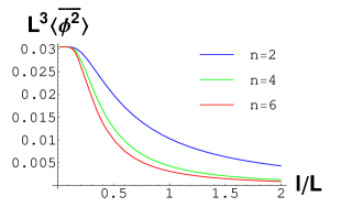
Figure 1: The vacuum expectation values of the square of the scalar field regulated as $L^{3}\langle\bar{\phi^{2}}\rangle$ for $m=0$ and $D=5$ are plotted against the cutoff length $l$ divided by the circumference $L$ of $S^{1}$ in the cases with $n=2$, $n=4$, and $n=6$ in Model A.

Figure 2: The vacuum expectation values of the square of the scalar field $l^{2}L\langle\bar{\phi^{2}}\rangle$ for $m=0$ and $D=5$ are plotted against the circumference $L$ of $S^{1}$ divided by the cutoff length $l$ in the cases with $n=1$, $n=2$, $n=4$, and $n=6$ in Model A. The black curve for the $n=1$ case indicates the usual case, i.e., the case that the cutoff length is set to zero.

Fig. 1 shows $L^{3}\langle\bar{\phi^{2}}\rangle$ in Model A as a function of $l/L$ for $m=0$ and $D=5$. Note that $\lim_{l\rightarrow 0}L^{3}\langle\bar{\phi^{2}}\rangle=\frac{\zeta_{R}(D-2)}{2\pi^{D/2}}$, where $\zeta_{R}(z)$ is Riemann’s zeta function, and it is $\approx 0.0343574$ for $D=5$. One can see that $L^{3}\langle\bar{\phi^{2}}\rangle$ monotonically decreases as $l$ increases. Fig. 2 shows $l^{2}L\langle\bar{\phi^{2}}\rangle$ in Model A as a function of $L/l$ for $m=0$ and $D=5$. The value of $l^{D-3}L\langle\bar{\phi^{2}}\rangle$ in $D$ dimensions at $L=0$ becomes finite if $n>\frac{D-1}{2}$, and is expressed by the following integral as for Model A:

$$\lim_{L/l\rightarrow 0}l^{D-3}L\langle\bar{\phi^{2}}\rangle=\frac{1}{(4\pi)^{D-1}}\int_{0}^{\infty}\frac{(1-e^{-t})^{n-1}}{t^{\frac{D-1}{2}}}dt\,.$$ (49)

For $D=5$ and $n=4$, $\lim_{L/l\rightarrow 0}l^{2}L\langle\bar{\phi^{2}}\rangle_{4}\approx 0.0054653$, while for $D=5$ and $n=6$, $\lim_{L/l\rightarrow 0}l^{2}L\langle\bar{\phi^{2}}\rangle_{6}\approx 0.00369362$.

For Model B, we find the expression of the vacuum expectation value $\langle\bar{\phi^{2}}\rangle=\bar{G}_{B}(0)$ in $\mathbf{R}^{D-1}\otimes S^{1}$ for $m=0$:

$$\langle\bar{\phi^{2}}\rangle=\frac{2l}{\pi^{\frac{D-1}{2}}}\sum_{q=1}^{\infty}\sum_{k=0}^{\infty}\frac{\Gamma\left(\frac{D-1}{2}\right)}{\left[q^{2}L^{2}+4\pi^{2}\left(k+\frac{1}{2}\right)^{2}l^{2}\right]^{\frac{D-1}{2}}}\,.$$ (50)

In Fig. 3, the value of $L^{3}\langle\bar{\phi^{2}}\rangle$ in Model B with $D=5$ and $m=0$ is plotted against $l/L$. Fig. 4 shows $l^{2}L\langle\bar{\phi^{2}}\rangle$ in Model B with $D=5$ and $m=0$ against $L/l$. The limit $L\rightarrow 0$ gives a finite value for $l^{D-3}L\langle\bar{\phi^{2}}\rangle$ in Model B, in arbitrary dimensions. It turns out to be

$$\lim_{L/l\rightarrow 0}l^{D-3}L\langle\bar{\phi^{2}}\rangle=\frac{1-2^{-(D-2)}}{\pi^{D-2}}\frac{\Gamma(\frac{D-2}{2})\zeta_{R}(D-2)}{\pi^{\frac{D-2}{2}}}\,.$$ (51)

In particular, we find $\lim_{L/l\rightarrow 0}l^{2}L\langle\bar{\phi^{2}}\rangle=\frac{7\zeta_{R}(3)}{16\pi^{4}}\approx 0.00539888$.

Figure 3: The vacuum expectation value regulated as $L^{2}\langle\bar{\phi^{2}}\rangle$ for $m=0$ and $D=5$ are plotted against the cutoff length $l$ divided by the circumference $L$ of $S^{1}$ in Model B.

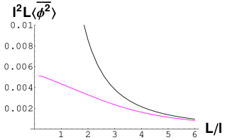
Figure 4: The vacuum expectation value regulated as $L^{2}\langle\bar{\phi^{2}}\rangle$ for $m=0$ and $D=5$ are plotted against the circumference $L$ of $S^{1}$ divided by the cutoff length $l$ in Model B. The black curve indicates the canonical case, i.e., the case that the cutoff length is set to zero and the other curve indicate the present UV modified case of Model B.

IV.2 The conical space

Next, we consider the vacuum expectation values in a conical space. A conical space, or a space with a conical singularity at the coordinate origin, is described by the metric

$$ds^{2}=\sum_{i=1}^{D-2}(dz^{i})^{2}+dr^{2}+\frac{r^{2}}{\nu^{2}}d\theta^{2}\,,$$ (52)

where $\nu$ is a constant greater than unity. This metric is equivalent to

$$ds^{2}=\sum_{i=1}^{D-2}(dz^{i})^{2}+dr^{2}+r^{2}d\tilde{\theta}^{2}\,,$$ (53)

where the range of $\tilde{\theta}$ is $0<\tilde{\theta}\leq 2\pi/\nu$. This metric adequately describes a locally flat Euclidean space except for the coordinate origin if $\nu\neq 1$.

The standard Green’s function in a conical space (without a fundamental length) is known Smith ; SH ; CKV ; Moreira . Because it is natural to take $\bar{G}(x,x^{\prime};M^{2})=G(x,x^{\prime};M^{2})-G(x,x^{\prime};M^{2})|_{\nu=1}$, we find KKSW

$$\bar{G}(x,x^{\prime};M^{2})=\bar{G}(r,r^{\prime},\varphi,\zeta;M^{2})$$ (54)

$$\equiv \int_{0}^{\infty}ds\,{\textstyle\frac{e^{-\frac{r^{2}+{r^{\prime}}^{2}+\zeta^{2}}{4s}-M^{2}s}}{2\pi(4\pi s)^{D/2}}}\int_{0}^{\infty}e^{-\frac{rr^{\prime}}{2s}\cosh v}\left[{\textstyle\frac{\nu\sin\nu(\tilde{\varphi}-\pi)}{\cosh\nu v-\cos\nu(\tilde{\varphi}-\pi)}-\frac{\nu\sin\nu(\tilde{\varphi}+\pi)}{\cosh\nu v-\cos\nu(\tilde{\varphi}+\pi)}}\right]dv\,,$$

where $x=(r,\theta,z^{i})$, $x^{\prime}=(r^{\prime},\theta^{\prime},z^{\prime i})$, and $\tilde{\varphi}=\tilde{\theta}-\tilde{\theta}^{\prime}=\varphi/\nu=(\theta-\theta^{\prime})/\nu$. Moreover, the vacuum expectation value of a single, canonical free scalar field squared can be rewritten as $\langle\bar{\phi^{2}}\rangle[M^{2}]=\bar{G}(x,x;M^{2})$. Using this, the vacuum expectation value is reduced to be in a similar form to (45) and equivalently

$$\langle\bar{\phi^{2}}\rangle=\sum_{k=0}^{n-1}c_{k}\bar{G}(x,x;M_{k}^{2})\,,$$ (55)

where we define $c_{0}\equiv 1$ and $M_{0}\equiv m$, in addition.

In the present case of the conical space, we thus find

$$\langle\bar{\phi^{2}}\rangle=\int_{0}^{\infty}ds\,\varrho(s){\frac{e^{-\frac{r^{2}}{2s}-m^{2}s}}{2\pi(4\pi s)^{D/2}}}\int_{0}^{\infty}e^{-\frac{r^{2}}{2s}\cosh v}\left[{\frac{-2\nu\sin\nu\pi}{\cosh\nu v-\cos\nu\pi}}\right]dv\,,$$ (56)

where we again used $\varrho(s)\equiv\sum_{k=0}^{n-1}c_{k}\exp[-s/\epsilon_{k}]$, which is already defined in the previous subsection.

Now, we can evaluate the vacuum expectation values of $\langle\bar{\phi^{2}}\rangle$ in Models A and B, very efficiently using these expressions (56). We assume that the original, unmodified theory is a free massless scalar theory ($m=0$).

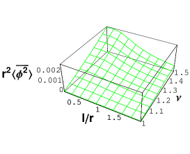
(a)                                         (b)                                         (c)

Figure 5: The vacuum expectation values regulated as $r^{2}\langle\bar{\phi^{2}}\rangle$ for $m=0$ and $D=4$ are plotted against the cutoff length $l$ divided by the distance from the origin $r$ in Model A, where (a) for $n=2$, (b) for $n=4$, and (c) for $n=6$.

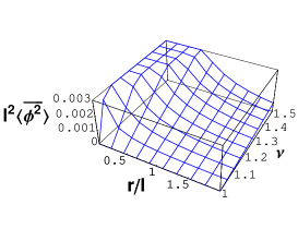
(a)                                         (b)                                         (c)

Figure 6: The vacuum expectation values regulated as $l^{2}\langle\bar{\phi^{2}}\rangle$ for $m=0$ and $D=4$ are plotted against the distance from the origin $r$ divided by the cutoff length $l$ in Model A, where (a) for $n=2$, (b) for $n=4$, and (c) for $n=6$. Note that the values diverge near $r/l\sim 0$ for $n=2$, the numerical values near $r/l$ are expressed up to a finite cut in the figure (a).

In Fig. 5, we illustrate the $l/r$ dependence of the vacuum expectation values of the square of the scalar field in Model A. The correction due to the scale $l$ has a little dependence on $n$ for a small $l/r$. Note that $\lim_{l/r\rightarrow 0}r^{2}\langle\bar{\phi^{2}}\rangle=\frac{\nu^{2}-1}{48\pi^{2}}$ Smith . The vacuum expectation values become small faster for larger $n$, though the changes are qualitatively the same.

In Figs. 6, we illustrate the $r/l$ dependence of the vacuum expectation values in Model A. In general, when $n>D/2$, the vacuum expectation values are finite at $r=0$. The value at the origin is finite as

$$\lim_{r/l\rightarrow 0}l^{D-2}\langle\bar{\phi^{2}}\rangle=\frac{(\nu-1)l^{D-2}}{(4\pi)^{D/2}}\int_{0}^{\infty}\frac{ds}{s^{D/2}}\varrho_{A}(s)=\frac{\nu-1}{(4\pi)^{D/2}}\int_{0}^{\infty}\frac{ds}{t^{D/2}}(1-e^{-t})^{n-1}\,.$$ (57)

For $D=4$ and $n=4$, this becomes $\approx 0.0054653\times(\nu-1)$, and for $D=4$ and $n=6$, this becomes $\approx 0.00369362\times(\nu-1)$.

(I)                                         (II)

Figure 7: (I) The vacuum expectation values for $m=0$ and $D=4$ regulated as $r^{2}\langle\bar{\phi^{2}}\rangle$ are plotted against the cutoff length $l$ divided by the distance from the origin $r$. (II) The vacuum expectation values regulated as $l^{2}\langle\bar{\phi^{2}}\rangle$ for $m=0$ and $D=4$ are plotted against the distance from the origin $r$ divided by the cutoff length $l$ in Model B.

In Fig. 7, we illustrate the $l/r$ dependence and the $r/l$ dependence of the vacuum expectation values in Model B. The values at $r=0$ are finite. In both cases, qualitative features are almost the same as in the case of Model A. The value at the origin is finite as

$$\lim_{r/l\rightarrow 0}l^{D-2}\langle\bar{\phi^{2}}\rangle=\frac{\nu-1}{(4\pi)^{D/2}}\int_{0}^{\infty}\frac{ds}{s^{D/2}}\varrho_{B}(s)=(\nu-1)\frac{1-2^{-(D-1)}}{\pi^{D-1}}\frac{\Gamma(\frac{D-1}{2})\zeta_{R}(D-1)}{\pi^{\frac{D-1}{2}}}\,.$$ (58)

For $D=4$, this becomes $\approx 0.00539888\times(\nu-1)$.

V Conclusion

In this paper, we first introduced a discrete heat kernel formulation of the Green’s function for a free scalar field, and considered the UV deformation that can be naturally obtained from it. The effective Lagrangian that derives this UV modified Green’s function has been found to be higher derivative theory. In the simplest case, it corresponds to a simple Pauli–Villars model, or, a Lee–Wick scalar field theory. In a further generalization, it was found that the present UV deformation yields a theory involving arbitrarily higher order derivatives, and the vacuum expectation values of the scalar field squared were evaluated in nontrivial spaces. We demonstrated that the cutoff length has an influence on the physical quantities at a short distance in the configuration space.

The advantage of using the heat kernel method is that we can keep the symmetry of the space (or break it at will). It is also easy to incorporate the effect of a constant external field (including spatial metric). On the other hand, one of the disadvantages is the handling of general interactions of dynamical fields. In addition, although the form of UV deformation is limited in our approach, it is also a problem that the sequence $\epsilon_{k}$ introduced in this paper has a wide range of arbitrariness other than the case of the two models.

To eliminate UV divergences completely, higher order derivatives that satisfy the conditions depending on the number of dimensions are required. Even if there is no divergence, a constant depending on the cutoff constant comes out. Therefore, some mechanism for canceling the finite contribution in the UV limit is still required. However, the present demonstration shows that the finite cutoff dependence of physical quantities occurs when the typical scale in the considered system is very close to the cutoff scale.

In the effective higher derivative theory, a scalar field with a negative norm appears, so the addition of interaction may bring about instability and violate unitarity in the Lorentzian spacetime. This is a subject that has been frequently addressed and has recently been actively discussed AP ; Anselmi , and in particular, infinite derivative theory is being studied in various situations Modesto ; BT ; BLM ; BLMTY . One of the models we have proposed (Model B) involves infinite derivatives, and the unitarity of the theory and its generalization should be studied further. Unfortunately, our current understanding has not led us to discuss the unitarity of the models presented in this paper in more detail. We consider that detailed discussions about nonlinear terms, i.e., interaction terms of fields are needed in the (infinitely) higher derivative theory, because it seems important to properly allocate higher order derivatives to the part of propagation and the part of interaction vertices.

It is interesting to study whether the theory with a basic cutoff scale can be derived naturally, for example from a model of quantum gravity, or not. That is a topic for the future, but one way might be to proceed with the tentative goal of deriving behavior like the simple models we examined here.

References

- (1) T. Padmanabhan, “Duality and zero-point length of spacetime”, Phys. Rev. Lett. 78 (1997) 1854. hep-th/9608182.
- (2) T. Padmanabhan, “Hypothesis of path integral duality. I. quantum gravitational corrections to the propagator”, Phys. Rev. D57 (1998) 6206.
- (3) T. Padmanabhan, “Principle of equivalence at Planck scales, QG in locally inertial frames and the zero-point-length of spacetime”, Gen. Rel. Grav. 52 (2020) 90. arXiv:2005.09677 [gr-qc].
- (4) T. Padmanabhan, “Probing the Planck scale: The modification of the time evolution operator due to the quantum structure of spacetime”, JHEP 2011 (2020) 013. arXiv:2006.06701 [gr-qc].
- (5) T. Padmanabhan, “Planck length: Lost+found”, Phys. Lett. B809 (2020) 135774.
- (6) T. Padmanabhan, “A class of QFTs with higher derivative field equations leading to standard dispersion relation for the particle excitations”, Phys. Lett. B811 (2020) 135912. arXiv:2011.04411 [hep-th].
- (7) K. Srinivasan, L. Sriramkumar and T. Padmanabhan, “Hypothesis of path integral duality. II. corrections to quantum field theoretic result”, Phys. Rev. D58 (1998) 044009. gr-qc/9710104.
- (8) D. Kothawala, L. Sriramkumar, S. Shankaranarayanan and T. Padmanabhan, “Path integral duality modified propagators in spacetimes with constant curvature”, Phys. Rev. D80 (2009) 044005. arXiv:0904.3217 [hep-th].
- (9) S. Abel and N. Dondi, “UV completion on the worldline”, JHEP 1907 (2019) 090. arXiv:1905.04258 [hep-th].
- (10) S. Abel, L. Buoninfante and A. Mazumdar, “Nonlocal gravity with worldline inversion symmetry”, JHEP 2001 (2020) 003. arXiv:1911.06697 [hep-th].
- (11) S. Abel and D. Lewis, “Worldline theories with towers of infinite states”, JHEP 2012 (2020) 069. arXiv:2007.07242 [hep-th].
- (12) W. Siegel, “String gravity at short distances”, hep-th/0309093.
- (13) N. Kan, M. Kuniyasu, K. Shiraishi and Z.-Y. Wu, “Vacuum expectation values in non-trivial background space from three types of UV improved Green’s functions”, Int. J. Mod. Phys. A36 (2021) 2150001. arXiv:2004.07537 [hep-th].
- (14) C. Itzykson and J.-B. Zuber, “Quantum Field Theory”, McGraw-Hill Book Company, New York, CA, 1980.
- (15) J. Collins, “Renormalization”, Cambridge Univ. Press, Cambridge, UK, 1984.
- (16) M. E. Peskin and D. V. Schroeder, “An Introduction to Quantum Field Theory”, Addison–Wesley Pub., Redwood, CA, 1995.
- (17) S. Shankaranarayanan and L. Sriramkumar, “Trans-Planckian corrections to the primordial spectrum in the infra-red and the ultra-violet”, Phys. Rev. D70 (2004) 123520. hep-th/0403236.
- (18) D. V. Vassilevich, “Heat kernel expansion: user’s manual”, Phys. Rep. 388 (2003) 279. hep-th/0306138.
- (19) R. Camporesi, “Harmonic analysis and propagators on homogeneous spaces”, Phys. Rep. 196 (1990) 1.
- (20) B. Grinstein, D. O’Connell and M. B. Wise, “The Lee–Wick standard model”, Phys. Rev. D77 (2008) 025012. arXiv:0704.1845 [hep-th].
- (21) C. D. Carone and R. F. Lebed, “A higher-derivative Lee–Wick standard model”, JHEP 0901 (2009) 043. arXive:0811.4150 [hep-ph].
- (22) T. D. Lee and G. C. Wick, “Negative metric and the unitarity of the S matrix”, Nucl. Phys. B9 (1969) 209.
- (23) S. A. Frolov and A. A. Slavnov, “An invariant regularization of the standard model”, Phys. Lett. B309 (1993) 344.
- (24) S. A. Frolov and A. A. Slavnov, “Removing fermion doublers in chiral gauge theories on the lattice”, Nucl. Phys. B411 (1994) 647. hep-lat/9303004.
- (25) K. Fujikawa, “Generalized Paulli–Villars regularization and the covariant form of anomalies”, Nucl. Phys. B428 (1994) 169. hep-th/9405166.
- (26) A. G. Smith, The Formation and Evolution of Cosmic Strings ed G. Gibbons, S. Hawking and T. Vachaspati (Cambridge: Cambridge University Press, 1989) p. 263.
- (27) K. Shiraishi and S. Hirenzaki, “Quantum aspects of self-interacting fields around cosmic strings”, Class. Quant. Grav. 9 (1992) 2277. arXiv:1812.01763 [hep-th].
- (28) G. Cognola, K. Kirsten and L. Vanzo, “Free and self-interacting scalar fields in the presence of conical singularities”, Phys. Rev. D49 (1994) 1029. hep-th/9308106.
- (29) E. S. Moreira Jnr., “Massive quantum fields in a conical background”, Nucl. Phys. B451 (1995) 365. hep-th/9502016.
- (30) D. Anselmi and M. Piva, “A new formulation of Lee–Wick quantum field theory”, JHEP 1706 (2017) 066. arXiv:1703.04584 [hep-th].
- (31) D. Anselmi, “The quest for purely virtual quanta: fakeons versus Feynman–Wheeler particles”, JHEP 2003 (2020) 142. arXiv:2001.01942 [hep-th].
- (32) L. Modesto, “Super-renormalizable quantum gravity”, Phys. Rev. D86 (2012) 044005. arXiv:1107.2403 [hep-th].
- (33) T. Biswas and S. Talaganis, “String-inspired infinite-derivative gravity: A brief overview”, Mod. Phys. Lett. A30 (2015) 1540009. arXiv:1412.4256 [gr-qc].
- (34) L. Buoninfante, G. Lambiase and A. Mazumdar, “Ghost-free infinite derivative quantum field theory”, Nucl. Phys. B944 (2019) 114646. arXiv:1805.03559 [hep-th].
- (35) L. Buoninfante, G. Lambiase, Y. Miyashita, W. Takebe and M. Yamaguchi, “Generalized ghost-free propagators in nonlocal field theory”, Phys. Rev. D101 (2020) 084019. arXiv:2001.07830 [hep-th].
- (36) F. Wu and M. Zhong, “The Lee–Wick fields out of gravity”, Phys. Lett. B659 (2008) 694.
- (37) F. Wu and M. Zhong, “TeV scale Lee–Wick fields out of large extra dimensional gravity”, Phys. Rev. D78 (2008) 085010.
- (38) A. Rodigast and T. Schuster, “No Lee–Wick fields out of gravity”, Phys. Rev. D79 (2009) 125017.