Microlocal analysis of generalized Radon transforms from scattering tomography
 

Abstract.

Here we present a novel microlocal analysis of generalized Radon transforms which describe the integrals of $L^{2}$ functions of compact support over surfaces of revolution of $C^{\infty}$ curves $q$. We show that the Radon transforms are elliptic Fourier Integral Operators (FIO) and provide an analysis of the left projections $\Pi_{L}$. Our main theorem shows that $\Pi_{L}$ satisfies the semi-global Bolker assumption if and only if $g=q^{\prime}/q$ is an immersion. An analysis of the visible singularities is presented, after which we derive novel Sobolev smoothness estimates for the Radon FIO. Our theory has specific applications of interest in Compton Scattering Tomography (CST) and Bragg Scattering Tomography (BST). We show that the CST and BST integration curves satisfy the Bolker assumption and provide simulated reconstructions from CST and BST data. Additionally we give example “sinusoidal” integration curves which do not satisfy Bolker and provide simulations of the image artefacts. The observed artefacts in reconstruction are shown to align exactly with our predictions.

1. Introduction

In this paper we present a new microlocal analysis of Radon transforms which describe the integrals of $L^{2}(\mathbb{R}^{n})$ functions of compact support over the surfaces of revolution of $q\in C^{\infty}((0,\infty))$. In 2-D the “surface of rotation” is the union of two curves which are the mirror images of one-another. We denote the union of the reflected curves as “broken-rays” (sometimes denoted by “V-lines” in the literature [5]) when $n=2$ and the surfaces of revolution as “generalized cones” when $n\geq 3$. We illustrate the scanning geometry and some example integration curves related to CST and BST in the $n=2$ case in figure 1. The Radon data is $n$-dimensional and comprised of an ($n-1$)-dimensional translation by ${\mathbf{x}}_{0}\in\mathbb{R}^{n-1}$ and a one-dimensional scaling by $E\in(0,\infty)$. We use the notation of [40] in BST, where classically $q=\sin\theta$ denotes the sine of the Bragg angle ($\theta$) and $E$ denotes the photon energy. Here we generalize the Radon transforms of [40] and analyze their stability microlocally. Our theory also has applications of interest in gamma ray source imaging in CST, specifically towards the broken-ray transforms of [1, 2, 5, 9, 10, 11, 27, 36], and the cone Radon transforms of [4, 13, 15, 20, 21, 23, 24, 25, 26, 28, 35, 37, 41].

Figure 1. The scanning geometry. The broken-ray curves displayed are $q_{C}(x)=x$ and $q_{B}(x)=\frac{x}{\sqrt{x^{2}+1}}$, which are of interest in CST and BST respectively. The curves are scaled by $E>0$, translated by $x_{0}$ along the $x$ axis and reflected in the line $x=x_{0}$. For example, in this case $x_{0}=3$, $E=2$ for $q_{B}$ and $E=\frac{1}{2}$ for $q_{C}$.

The generalized Radon transforms considered here are shown to be elliptic FIO order $\frac{1-n}{2}$, and we give an analysis of the left projections $\Pi_{L}$. Our main theorem proves that $\Pi_{L}$ satisfies the semi-global Bolker assumption (i.e. $\Pi_{L}$ is an embedding) if and only if the quotient function $g=q^{\prime}/q$ is an immersion. Then, we consider the visible singularities in the Radon data and provide Sobolev space estimates for the level of smoothing of the target singularities. This serves to reduce the microlocal and Sobolev analysis of our $n$-dimensional Radon FIO to the injectivity analysis of the one-dimensional function $g$.

We consider two applications of our theory that are of interest, namely Compton camera imaging in CST and crystalline structure imaging in BST. We show that the CST and BST integration curves satisfy the conditions of our theorems, which, by implication, proves that the CST and BST operators are elliptic FIO which satisfy Bolker. Additionally we give example “sinusoidal” $q$ for which the corresponding transforms are shown to violate the Bolker assumption. In this case there are artefacts appearing along the $q$ curves at the points where $g=q^{\prime}/q$ is non-injective. Using the $g$ mapping, we are able to predict precisely the locations of the artefacts in reconstruction. To verify our theory, we present simulated reconstructions of a delta function and a characteristic function on a disc from CST, BST and sinusoidal data. The predicted artifacts are shown to align exactly with those observed in reconstruction.

The literature includes the microlocal analysis of broken-ray transforms in [5, 34] and cone Radon transforms in [34, 41]. In [5], the authors analyze the boundary artefacts in reconstruction from broken-ray (denoted V-lines in [5]) integrals, which occur along broken-ray curves at the edge of the data set. A smooth cut off in the frequency domain is later introduced to combat the boundary artefacts. Proof of FIO and injectivity analysis of the $\Pi_{L}$ is not considered however. We aim to cover this here for the broken-ray transform. In [41], the author considers the five-dimensional set of cone integrals in $\mathbb{R}^{3}$, where the cone vertices are constrained to smooth 2-D surfaces $\mathcal{S}$ in $\mathbb{R}^{3}$. In [41, Proposition 4] the normal operator of the cone transform is proven to be an elliptic Pseudo Differential Operator (PDO) order $-2$ (under certain visibility assumptions), thus implying that the Bolker assumption is satisfied. In contrast, for ${{\mathbb{R}}^{3}}$, we consider the three-dimensional subset of the Radon data when the surface of cone vertices $\mathcal{S}=\mathbb{R}^{2}$ is the $(u_{1},u_{2})$ plane and the axis of rotation has direction $\beta=(0,1)$ (using the notation in [41, Example 1]). We prove that the Bolker assumption is satisfied here with limited data, and our surfaces of integration are more general than cones. In [34, section 4] the $n$-dimensional case for the cone transform is analyzed microlocally; the Radon integrals are taken over the full set of cones in $\mathbb{R}^{n}$, and the data set is $2n$-dimensional. In [34, Theorem 14] it is proven that the normal operator of the $2n$-dimensional cone transform is a PDO. We consider the $n$-dimensional subset of the Radon data where (using the notation of [34]) ${\mathbf{u}}\in\{u_{n}=0\}$ is constrained to the $(u_{1},\ldots,u_{n-1})$ plane, and the axis of rotation has direction $\beta=(\mathbf{0},1)$. That is, we consider the vertical (i.e. $\beta=(\mathbf{0},1)$) cones with vertices on $\{u_{n}=0\}$. The results of [34, Theorem 14] are not sufficient to prove Bolker with limited data. The vertical cone Radon transform is also considered in [37], but no microlocal analysis is given. We aim to cover this important limited data case here. In addition, our theorems are valid, not only for cones, but for general surfaces of revolution satisfying (3.5).

Our transform is a Radon transform on surfaces of revolution that are generated by translation by directions in the $x_{n}=0$ plane. Radon transforms on surfaces of revolution have been considered in the pure mathematical community, such as [6, 22], but in those articles, the surfaces are generated by rotation about the origin not translation in a hyperplane.

In [40] Radon models (denoted by the “Bragg transform”) are introduced for crystalline structure imaging in BST and airport baggage screening. The curves of integration in BST are illustrated by $q_{B}$ in figure 1. Injectivity proofs and explicit inversion formulae are provided for the Bragg transform in [40, Theorem 4.1]. The stability analysis is not covered however. We aim to address the stability aspects of the Bragg transform here from a microlocal perspective.

The remainder of this paper is organized as follows. In section 2 we recall some notation and definitions from microlocal analysis which will be used in our theorems. In section 3 we define the generalized cone Radon transform $R$, which describes the integrals of $L^{2}$ functions over the surfaces of revolution of smooth $q$. We prove that $R$ is an elliptic FIO order $\frac{1-n}{2}$ and provide expression for the left projection $\Pi_{L}$. We then go on to prove our main theorem, which shows that $\Pi_{L}$ is an injective immersion if and only if $g=q^{\prime}/q$ is an immersion. The smoothing in Sobolev norms is later explained in section 3.3. In section 4 we show that the curves of integration in CST and BST (as displayed in figure 1) satisfy the conditions of our theorems, and we provide simulated reconstructions from CST and BST data. Additionally, in example 4.3, we give example “sinusoidal” $q$ with $g$ not an immersion, thus violating Bolker. We simulate the artefacts in reconstruction from these sinusoidal integrals. The observed artefacts are shown to align exactly with our predictions and the theory of section 3.

2. Microlocal definitions

We next provide some notation and definitions. Let $X$ and $Y$ be open subsets of ${{\mathbb{R}}^{n}}$. Let $\mathcal{D}(X)$ be the space of smooth functions compactly supported on $X$ with the standard topology and let $\mathcal{D}^{\prime}(X)$ denote its dual space, the vector space of distributions on $X$. Let $\mathcal{E}(X)$ be the space of all smooth functions on $X$ with the standard topology and let $\mathcal{E}^{\prime}(X)$ denote its dual space, the vector space of distributions with compact support contained in $X$. Finally, let $\mathcal{S}({{\mathbb{R}}^{n}})$ be the space of Schwartz functions, that are rapidly decreasing at $\infty$ along with all derivatives. See [33] for more information.

Definition 2.1 ([17, Definition 7.1.1]).

For a function $f$ in the Schwartz space $\mathcal{S}(\mathbb{R}^{n})$, we define the Fourier transform and its inverse as

(2.1) $$\mathcal{F}f({\boldsymbol{\xi}})=\int_{\mathbb{R}^{n}}e^{-i{\mathbf{x}}\cdot{\boldsymbol{\xi}}}f({\mathbf{x}})\mathrm{d}{\mathbf{x}},\qquad\mathcal{F}^{-1}f({\mathbf{x}})=(2\pi)^{-n}\int_{\mathbb{R}^{n}}e^{i{\mathbf{x}}\cdot{\boldsymbol{\xi}}}f({\boldsymbol{\xi}})\mathrm{d}{\boldsymbol{\xi}}.$$

We use the standard multi-index notation: if $\alpha=(\alpha_{1},\alpha_{2},\dots,\alpha_{n})\in\left\{0,1,2,\dots\right\}^{n}$ is a multi-index and $f$ is a function on ${{\mathbb{R}}^{n}}$, then

$$\partial^{\alpha}f=\left(\frac{\partial}{\partial x_{1}}\right)^{\alpha_{1}}\left(\frac{\partial}{\partial x_{2}}\right)^{\alpha_{2}}\cdots\left(\frac{\partial}{\partial x_{n}}\right)^{\alpha_{n}}f.$$

If $f$ is a function of $({\mathbf{y}},{\mathbf{x}},\mathbf{s})$ then $\partial^{\alpha}_{\mathbf{y}}f$ and $\partial^{\alpha}_{\mathbf{s}}f$ are defined similarly.

We identify cotangent spaces on Euclidean spaces with the underlying Euclidean spaces, so we identify $T^{*}(X)$ with $X\times{{\mathbb{R}}^{n}}$.

If $\phi$ is a function of $({\mathbf{y}},{\mathbf{x}},\mathbf{s})\in Y\times X\times{{\mathbb{R}}}^{N}$ then we define $\mathrm{d}_{{\mathbf{y}}}\phi=\left(\frac{\partial\phi}{\partial y_{1}},\frac{\partial\phi}{\partial y_{2}},\cdots,\frac{\partial\phi}{\partial y_{n}}\right)$, and $\mathrm{d}_{\mathbf{x}}\phi$ and $\mathrm{d}_{\mathbf{s}}\phi$ are defined similarly. We let $\mathrm{d}\phi=\left(\mathrm{d}_{{\mathbf{y}}}\phi,\mathrm{d}_{{\mathbf{x}}}\phi,\mathrm{d}_{\mathbf{s}}\phi\right)$.

We use the convenient notation that if $A\subset{{\mathbb{R}}}^{m}$, then $\dot{A}=A\setminus\mathbf{0}$.

The singularities of a function and the directions in which they occur are described by the wavefront set [8, page 16]:

Definition 2.2.

Let $X$ Let an open subset of ${{\mathbb{R}}^{n}}$ and let $f$ be a distribution in $\mathcal{D}^{\prime}(X)$. Let $({\mathbf{x}}_{0},{\boldsymbol{\xi}}_{0})\in X\times{\dot{{\mathbb{R}}^{n}}}$. Then $f$ is smooth at ${\mathbf{x}}_{0}$ in direction ${\boldsymbol{\xi}_{0}}$ if there exists a neighbourhood $U$ of ${\mathbf{x}}_{0}$ and $V$ of ${\boldsymbol{\xi}}_{0}$ such that for every $\phi\in\mathcal{D}(U)$ and $N\in\mathbb{R}$ there exists a constant $C_{N}$ such that for all ${\boldsymbol{\xi}}\in V$,

(2.2) $$\left|\mathcal{F}(\phi f)(\lambda{\boldsymbol{\xi}})\right|\leq C_{N}(1+\left|\lambda\right|)^{-N}.$$

The pair $({\mathbf{x}}_{0},{\boldsymbol{\xi}_{0}})$ is in the wavefront set, $\mathrm{WF}(f)$, if $f$ is not smooth at ${\mathbf{x}}_{0}$ in direction ${\boldsymbol{\xi}_{0}}$.

This definition follows the intuitive idea that the elements of $\mathrm{WF}(f)$ are the point–normal vector pairs above points of $X$ at which $f$ has singularities. For example, if $f$ is the characteristic function of the unit ball in $\mathbb{R}^{3}$, then its wavefront set is $\mathrm{WF}(f)=\{({\mathbf{x}},t{\mathbf{x}}):{\mathbf{x}}\in S^{2},t\neq 0\}$, the set of points on a sphere paired with the corresponding normal vectors to the sphere.

The wavefront set of a distribution on $X$ is normally defined as a subset the cotangent bundle $T^{*}(X)$ so it is invariant under diffeomorphisms, but we do not need this invariance, so we will continue to identify $T^{*}(X)=X\times{{\mathbb{R}}^{n}}$ and consider $\mathrm{WF}(f)$ as a subset of $X\times{\dot{{\mathbb{R}}^{n}}}$.

Definition 2.3 ([17, Definition 7.8.1]).

We define $S^{m}(Y\times X\times\mathbb{R}^{N})$ to be the set of $a\in\mathcal{E}(Y\times X\times\mathbb{R}^{N})$ such that for every compact set $K\subset Y\times X$ and all multi–indices $\alpha,\beta,\gamma$ the bound

$$\left|\partial^{\gamma}_{{\mathbf{y}}}\partial^{\beta}_{{\mathbf{x}}}\partial^{\alpha}_{{\boldsymbol{\sigma}}}a({\mathbf{y}},{\mathbf{x}},{\boldsymbol{\sigma}})\right|\leq C_{K,\alpha,\beta,\gamma}(1+\left\lVert{\boldsymbol{\sigma}}\right\rVert)^{m-|\alpha|},\ \ \ ({\mathbf{y}},{\mathbf{x}})\in K,\ {\boldsymbol{\sigma}}\in\mathbb{R}^{N},$$

holds for some constant $C_{K,\alpha,\beta,\gamma}>0$.

The elements of $S^{m}$ are called symbols of order $m$. Note that these symbols are sometimes denoted $S^{m}_{1,0}$. The symbol $a\in S^{m}(Y,X,{{\mathbb{R}}}^{N})$ is elliptic if for each compact set $K\subset Y\times X$, there is a $C_{K}>0$ and $M>0$ such that

(2.3) $$\left|a({\mathbf{y}},{\mathbf{x}},{\boldsymbol{\sigma}})\right|\geq C_{K}(1+\left\lVert{\boldsymbol{\sigma}}\right\rVert)^{m},\ \ \ ({\mathbf{y}},{\mathbf{x}})\in K,\ \left\lVert{\boldsymbol{\sigma}}\right\rVert\geq M.$$

Definition 2.4 ([18, Definition 21.2.15]).

A function $\phi=\phi({\mathbf{y}},{\mathbf{x}},{\boldsymbol{\sigma}})\in\mathcal{E}(Y\times X\times\dot{\mathbb{R}^{N}})$ is a phase function if $\phi({\mathbf{y}},{\mathbf{x}},\lambda{\boldsymbol{\sigma}})=\lambda\phi({\mathbf{y}},{\mathbf{x}},{\boldsymbol{\sigma}})$, $\forall\lambda>0$ and $\mathrm{d}\phi$ is nowhere zero. A phase function is clean if the critical set $\Sigma_{\phi}=\{({\mathbf{y}},{\mathbf{x}},{\boldsymbol{\sigma}})\ :\ \mathrm{d}_{\boldsymbol{\sigma}}\phi({\mathbf{y}},{\mathbf{x}},{\boldsymbol{\sigma}})=0\}$ is a smooth manifold with tangent space defined by $\mathrm{d}\left(\mathrm{d}_{\boldsymbol{\sigma}}\phi\right)=0$.

By the implicit function theorem the requirement for a phase function to be clean is satisfied if $\mathrm{d}\left(\mathrm{d}_{\boldsymbol{\sigma}}\phi\right)$ has constant rank.

Definition 2.5 ([18, Definition 21.2.15] and [19, section 25.2]).

Let $X$ and $Y$ be open subsets of ${{\mathbb{R}}^{n}}$. Let $\phi\in\mathcal{E}\left(Y\times X\times{{{\mathbb{R}}}}^{N}\right)$ be a clean phase function. In addition, we assume that $\phi$ is nondegenerate in the following sense:

$$\mathrm{d}_{{\mathbf{y}},{\boldsymbol{\sigma}}}\phi \mathrm{d}_{{\mathbf{x}},{\boldsymbol{\sigma}}}\phi$$ and are never zero.

The critical set of $\phi$ is

$$\Sigma_{\phi}=\{({\mathbf{y}},{\mathbf{x}},{\boldsymbol{\sigma}})\in Y\times X\times\dot{\mathbb{R}^{N}}:\mathrm{d}_{{\boldsymbol{\sigma}}}\phi=0\}.$$

The canonical relation parametrised by $\phi$ is defined as

(2.4) $$\mathcal{C}= \left\{\left(\left({\mathbf{y}},\mathrm{d}_{{\mathbf{y}}}\phi({\mathbf{y}},{\mathbf{x}},{\boldsymbol{\sigma}})\right);\left({\mathbf{x}},-\mathrm{d}_{{\mathbf{x}}}\phi({\mathbf{y}},{\mathbf{x}},{\boldsymbol{\sigma}})\right)\right):({\mathbf{y}},{\mathbf{x}},{\boldsymbol{\sigma}})\in\Sigma_{\phi}\right\},$$

Definition 2.6.

Let $X$ and $Y$ be open subsets of ${{\mathbb{R}}^{n}}$. A Fourier integral operator (FIO) of order $m+N/2-n/2$ is an operator $A:\mathcal{D}(X)\to\mathcal{D}^{\prime}(Y)$ with Schwartz kernel given by an oscillatory integral of the form

(2.5) $$K_{A}({\mathbf{y}},{\mathbf{x}})=\int_{\mathbb{R}^{N}}e^{i\phi({\mathbf{y}},{\mathbf{x}},{\boldsymbol{\sigma}})}a({\mathbf{y}},{\mathbf{x}},{\boldsymbol{\sigma}})\mathrm{d}{\boldsymbol{\sigma}},$$

where $\phi$ is a clean nondegenerate phase function and $a$ is a symbol in $S^{m}(Y\times X\times\mathbb{R}^{N})$. The canonical relation of $A$ is the canonical relation of $\phi$ defined in (2.4).

The FIO $A$ is elliptic if its symbol is elliptic.

This is a simplified version of the definition of FIO in [7, section 2.4] or [19, section 25.2] that is suitable for our purposes since our phase functions are global. Because we assume phase functions are nondegenerate, our FIO can be extended from as maps from $\mathcal{D}(X)$ to $\mathcal{E}(Y)$ to maps from $\mathcal{E}^{\prime}(X)$ to $\mathcal{D}^{\prime}(Y)$, and sometimes larger sets. For general information about FIOs see [7, 19, 18].

The composition of sets is defined as follows. Let $X$ and $Y$ be sets and let $A\subset X$ and $B\subset Y\times X$ the composition

$$B\circ A =\left\{y\in Y\hskip 0.85358pt:\hskip 0.85358pt\exists x\in X,\ (y,x)\in B\right\}$$

$$B^{t} =\left\{(x,y)\hskip 0.85358pt:\hskip 0.85358pt(y,x)\in B\right\}.$$

The Hörmander-Sato Lemma provides the relationship between the wavefront set of distributions and their images under FIO.

Theorem 2.7 ([17, Theorem 8.2.13]).

Let $f\in\mathcal{E}^{\prime}(X)$ and let $F:\mathcal{E}^{\prime}(X)\to\mathcal{D}^{\prime}(Y)$ be an FIO with canonical relation $\mathcal{C}$. Then, $\mathrm{WF}(Ff)\subset\mathcal{C}\circ\mathrm{WF}(f)$.

Definition 2.8.

Let $\mathcal{C}\subset T^{*}(Y\times X)$ be the canonical relation associated to the FIO $A:\mathcal{E}^{\prime}(X)\to\mathcal{D}^{\prime}(Y)$. Let $\Pi_{L}$ and $\Pi_{R}$ denote the natural left- and right-projections of $\mathcal{C}$, projecting onto the appropriate coordinates: $\Pi_{L}:\mathcal{C}\to T^{*}(Y)$ and $\Pi_{R}:\mathcal{C}\to T^{*}(X)$.

Because $\phi$ is nondegenerate, the projections do not map to the zero section.

If a FIO $\mathcal{F}$ satisfies our next definition, then $\mathcal{F}^{*}\mathcal{F}$ (or, if $\mathcal{F}$ does not map to $\mathcal{E}^{\prime}(Y)$, then $\mathcal{F}^{*}\psi\mathcal{F}$ for an appropriate cutoff $\psi$) is a pseudodifferential operator [14, 31].

Definition 2.9.

Let $\mathcal{F}:\mathcal{E}^{\prime}(X)\to\mathcal{D}^{\prime}(Y)$ be a FIO with canonical relation $\mathcal{C}$ then $\mathcal{F}$ (or $\mathcal{C}$) satisfies the semi-global Bolker Assumption if the natural projection $\Pi_{Y}:\mathcal{C}\to T^{*}(Y)$ is an embedding (injective immersion).

3. The Main Theorem

In this section we define our transform and give conditions under which our transform satisfies the Bolker Assumption. We consider a Radon transform in ${{\mathbb{R}}^{n}}$ that is a generalization of the transforms studied in [5, 35, 40, 41]. This transform will integrate on surfaces of rotation with vertex on the $x_{n}=0$ hyperplane.

We start with a function that will define the surfaces.

(3.1) $$\begin{gathered}\text{Let $q:[0,\infty)\to[0,\infty)$ be continuous on $[0,\infty)$, $C^{\infty}$ on $(0,\infty)$, }\\ \text{$q(0)=0$, and $q(r)>0$ if $r>0$.}\end{gathered}$$

If ${\mathbf{x}}=(x_{1},x_{2},\dots,x_{n})\in{{\mathbb{R}}^{n}}$ then we let ${\mathbf{x}}^{\prime}=(x_{1},x_{2},\dots,x_{n-1})\in{\mathbb{R}^{n-1}}$ so ${\mathbf{x}}=({\mathbf{x}}^{\prime},x_{n})$. Now, let $X=\left\{({\mathbf{x}}^{\prime},x_{n})\hskip 0.85358pt:\hskip 0.85358pt{\mathbf{x}}^{\prime}\in{\mathbb{R}^{n-1}},x_{n}\in(0,\infty)\right\}$ denote the half-space $x_{n}>0$ in ${{\mathbb{R}}^{n}}$. Let $Y=(0,\infty)\times{\mathbb{R}^{n-1}}$. Then, for $(E,\mathbf{x}_{0})\in Y$, the surface of integration of our Radon transform is given by

(3.2) $$S(E,\mathbf{x}_{0})=\left\{({\mathbf{x}}^{\prime},x_{n})\hskip 0.85358pt:\hskip 0.85358ptx_{n}=Eq\left(\left\lVert{\mathbf{x}}^{\prime}-\mathbf{x}_{0}\right\rVert\right)\ {\mathbf{x}}^{\prime}\in{\mathbb{R}^{n-1}}\setminus\left\{\mathbf{x}_{0}\right\}\right\}.$$

Note that $S(E,\mathbf{x}_{0})$ has axis of rotation $\{(\mathbf{x}_{0},x_{n})\hskip 0.85358pt:\hskip 0.85358ptx_{n}>0\}$ and vertex at $(\mathbf{x}_{0},0)$ (which is not in $S(E,\mathbf{x}_{0})$). The surface $S(E,\mathbf{x}_{0})$ is characterized by the equation

(3.3) $$\begin{gathered}\Psi(E,\mathbf{x}_{0},({\mathbf{x}}^{\prime},x_{n}))=0\text{\ \ where}\\ \Psi(E,\mathbf{x}_{0},({\mathbf{x}}^{\prime},x_{n})):=x_{n}-Eq\left(\left\lVert{\mathbf{x}}^{\prime}-\mathbf{x}_{0}\right\rVert\right)\end{gathered}$$

The generalized cone Radon transform is given, for $f\in L^{2}_{c}(X)$, by

(3.4) $$Rf(E,\mathbf{x}_{0}) =\int_{{\mathbf{x}}\in S(E,\mathbf{x}_{0})}f({\mathbf{x}})\mathrm{d}S({\mathbf{x}})$$

$$=\int_{({\mathbf{x}},x_{n})\in X}f({\mathbf{x}}^{\prime},x_{n})\,\left\lVert\nabla_{\mathbf{x}}\Psi\right\rVert\,\delta\left(\Psi(E,\mathbf{x}_{0},({\mathbf{x}}^{\prime},x_{n}))\right)\mathrm{d}{\mathbf{x}}^{\prime}\,\mathrm{d}x_{n}$$

where we use [29, eq. (1)] and the relation of the transform $M_{\Psi}$ in that article to $R$ (see also [17, §6.1]). Thus, $Rf(E,\mathbf{x}_{0})$ integrates $f$ over the surface of rotation $S(E,\mathbf{x}_{0})$ in surface area measure.

Our first main theorem allows us to analyze mapping properties of $R$ microlocally and in Sobolev space.

Theorem 3.1.

Let $q:[0,\infty)\to[0,\infty)$ satisfy (3.1). Then, the associated generalized cone Radon transform $R$ is an elliptic FIO of order $\frac{1-n}{2}$.

Let $g=q^{\prime}/q$ and assume $g:(0,\infty)\to(0,\infty)$. Then, the transform $R$ satisfies the Bolker assumption if and only if

(3.5) $$g^{\prime}(r)\neq 0 r\in(0,\infty) g$$ for all (i.e., is an immersion).

This condition is equivalent to $qq^{\prime\prime}-(q^{\prime})^{2}$ being nowhere zero for $r\in(0,\infty)$.

Remark 3.2.

First, note that our theorems are valid for all Radon transforms defined on surfaces $S(E,\mathbf{x}_{0})$ for which $q$ and $g$ satisfy the conditions in Theorem 3.1 and the weights on the surfaces are smooth and nowhere zero. This is true because our proofs use microlocal analysis, which does not depend on the specific weight. Ellipticity of the operator follows because the weight is assumed to be nowhere zero.

Let $\mathcal{C}$ be the canonical relation of $R$. For the Bolker Assumption to hold, $\Pi_{L}:\mathcal{C}\to T^{*}(Y)$ needs to be both injective and immersive. In our proof, we will show that (3.5) is equivalent to $\Pi_{L}$ being immersive. We will also show that the condition

(3.6) $$g:(0,\infty)\to(0,\infty)\ \,\text{is injective}$$

is equivalent to $\Pi_{L}$ being injective. However, condition (3.5) implies this new condition (3.6) for the following reason: if $g^{\prime}$ is never $0$ then $g$ must be strictly monotonic because the domain of $g$, $(0,\infty)$, is connected.

We will first prove this theorem in ${{\mathbb{R}}^{2}}$ since this provides the main ideas. Then, we provide the general proof for ${{\mathbb{R}}^{n}}$.

3.1. Proof of Theorem 3.1 in ${{\mathbb{R}}^{2}}$

In this case the “surface of rotation” $S(E,x_{0})$ consists of two curves that are mirror images of each other, so we will introduce two Radon transforms. Throughout this section we use the coordinates $(E,x_{0},x_{1},x_{2},\sigma)\in Y\times X\times\dot{\mathbb{R}}$.

Define

$$D_{j}=D_{j}(x_{0})=\left\{(x_{1},x_{2})\hskip 0.85358pt:\hskip 0.85358pt{(-1)^{j}(x_{1}-x_{0})}>0,x_{2}>0\right\}$$

and let $\Psi_{j}(E,x_{0},x_{1},x_{2})=x_{2}-Eq({(-1)^{j}(x_{1}-x_{0})})$. Then, for $f\in L^{2}_{c}(X)$, we define the transforms $R_{j}$, for $j=1,2$, as

(3.7) $$R_{j}f(E,x_{0}) =\int_{D_{j}(x_{0})}\left\lVert\nabla_{{\mathbf{x}}}\Psi_{j}(E,x_{0},{\mathbf{x}})\right\rVert\delta(x_{2}-Eq({(-1)^{j}}(x_{1}-x_{0}))f({\mathbf{x}})\mathrm{d}{\mathbf{x}}$$

$$=\int_{-\infty}^{\infty}\int_{D_{j}(x_{0})}a({\mathbf{x}},E,x_{0})e^{\Phi_{j}(E,x_{0},{\mathbf{x}},\sigma)}f({\mathbf{x}})\mathrm{d}{\mathbf{x}}\mathrm{d}\sigma,$$

where

$$\Phi_{j}(E,x_{0},{\mathbf{x}},\sigma)=\sigma\left(x_{2}-Eq({(-1)^{j}}(x_{1}-x_{0}))\right),$$

and

(3.8) $$\begin{split}a({\mathbf{x}},E,x_{0})&=\left\lVert\nabla_{{\mathbf{x}}}\Psi_{j}(E,x_{0},{\mathbf{x}})\right\rVert\\ &=\sqrt{1+E^{2}(q^{\prime}((-1)^{j}(x_{1}-x_{0})))^{2}}.\end{split}$$

To get the second line of (3.7) we use the Fourier representation of the delta function. Then, in ${{\mathbb{R}}^{2}}$, the Radon transform $R$ of (3.4) can be written

(3.9) $$Rf(E,x_{0})=R_{1}f(E,x_{0})+R_{2}f(E,x_{0}).$$

It can be shown that the phase function $\Phi_{j}$ is non-degenerate (see definition 2.4). The calculation of non-degeneracy is left to the reader.

The amplitude $a$ is smooth, never zero, and not dependent on the phase variable $\sigma$. Further the partial derivatives of $a$, of all orders, are bounded on any compact set. Therefore $a$ is a symbol order zero. It follows that the $R_{j}$ and $R=R_{1}+R_{2}$ are elliptic FIO order $O(R),O(R_{j})=0+\frac{1}{2}-\frac{2}{2}=-\frac{1}{2}$, using the formula of Definition 2.6.

Let $\mathcal{D}_{j}=(0,\infty)\times\left\{(x_{0},x_{1})\in{{\mathbb{R}}^{2}}\hskip 0.85358pt:\hskip 0.85358pt(-1)^{j}(x_{1}-x_{0})>0\right\}\times\dot{\mathbb{R}}$. Then the canonical relations of the $R_{j}$ are

$$\mathcal{C}_{j}= \Big{\{}\big{(}\overbrace{(E,x_{0})}^{{\mathbf{y}}},\overbrace{-\sigma q({(-1)^{j}}(x_{1}-x_{0})),{(-1)^{j}}\sigma Eq^{\prime}({(-1)^{j}}(x_{1}-x_{0}))}^{\mathrm{d}_{{\mathbf{y}}}\Phi_{j}};$$

$$\qquad{\mathbf{x}},\underbrace{{(-1)^{j}}\sigma Eq^{\prime}({(-1)^{j}(x_{1}-x_{0})}),-\sigma}_{-\mathrm{d}_{{\mathbf{x}}}\Phi_{j}}\big{)}\hskip 0.85358pt:\hskip 0.85358pt(E,x_{0},x_{1},\sigma)\in\mathcal{D}_{j},x_{2}=Eq({(-1)^{j}(x_{1}-x_{0})})\Big{\}}$$

In these coordinates using $\mathcal{D}_{j}$, the left projection $\Pi^{(j)}_{L}:\mathcal{D}_{j}\to\Pi^{(j)}_{L}(\mathcal{D}_{j})$ of $R_{j}$ is

$$\Pi_{L}^{(j)}(E,x_{0},x_{1},\sigma)=(E,x_{0},-\sigma q({(-1)^{j}}(x_{1}-x_{0})),{(-1)^{j}}\sigma Eq^{\prime}({(-1)^{j}}(x_{1}-x_{0}))).$$

Then the left projection $\Pi_{L}:\mathcal{D}_{1}\cup\mathcal{D}_{2}\to\Pi_{L}\left(\mathcal{D}_{1}\cup\mathcal{D}_{2}\right)$ of $R$ is defined by $\Pi_{L}=\Pi^{(1)}_{L}$ on $\mathcal{D}_{1}$, and $\Pi_{L}=\Pi^{(2)}_{L}$ on $\mathcal{D}_{2}$. The canonical relation of $R$ is the disjoint union $\mathcal{C}=\mathcal{C}_{1}\cup\mathcal{C}_{2}$.

We will now show that condition 3.5 is equivalent to $\Pi_{L}$ an immersion. To do this we consider the derivatives of the $\Pi^{(j)}_{L}$,

(3.10) $$D\Pi^{(j)}_{L}=\begin{pmatrix}1&0&0&0\\ 0&1&0&0\\ a_{3,1}&a_{3,2}&{(-1)^{j+1}}\sigma q^{\prime}({(-1)^{j}(x_{1}-x_{0})})&-q({(-1)^{j}(x_{1}-x_{0})})\\ a_{4,1}&a_{4,2}&\sigma Eq^{\prime\prime}({(-1)^{j}(x_{1}-x_{0})})&{(-1)^{j}}Eq^{\prime}({(-1)^{j}(x_{1}-x_{0})})\end{pmatrix}.$$

The determinant is

(3.11) $$\begin{split}\text{det}D\Pi^{(j)}_{L}&=\text{det}\begin{pmatrix}{(-1)^{j+1}}\sigma q^{\prime}({(-1)^{j}(x_{1}-x_{0})})&-q({(-1)^{j}(x_{1}-x_{0})})\\ \sigma Eq^{\prime\prime}({(-1)^{j}(x_{1}-x_{0})})&{(-1)^{j}}Eq^{\prime}({(-1)^{j}(x_{1}-x_{0})})\end{pmatrix}\\ &=\sigma E\left(q({(-1)^{j}(x_{1}-x_{0})})q^{\prime\prime}({(-1)^{j}(x_{1}-x_{0})})-q^{\prime}({(-1)^{j}(x_{1}-x_{0})})^{2}\right),\end{split}$$

which is non-vanishing if and only if

(3.12) $$q(x_{1})q^{\prime\prime}(x_{1})-q^{\prime}(x_{1})^{2}\neq 0,\ \ \ \forall x_{1}\in\dot{\mathbb{R}}.$$

Now

$$g^{\prime}(x_{1})=\frac{q^{\prime\prime}(x_{1})}{q(x_{1})}-\frac{q^{\prime}(x_{1})^{2}}{q^{2}(x_{1})}=0\iff q(x_{1})q^{\prime\prime}(x_{1})-q^{\prime}(x_{1})^{2}=0$$

for $x\in\dot{\mathbb{R}}$. The results follows.

We now show that condition 3.6 is equivalent to $\Pi_{L}$ injective. We first consider the implication $\ref{g}\implies\Pi_{L}\ \ \text{injective}$.

Let $g$ be injective, and let $(E_{1},x_{0},x_{1},\sigma_{1}),(E_{2},x^{\prime}_{0},x^{\prime}_{1},\sigma_{2})\in\mathcal{D}_{j}$ be such that
$\Pi^{(j)}_{L}(E_{1},x_{0},x_{1},\sigma_{1})=\Pi^{(j)}_{L}(E_{2},x^{\prime}_{0},x^{\prime}_{1},\sigma_{2})$. Then $E_{1}=E_{2}=E$, $x_{0}=x^{\prime}_{0}$, and

(3.13) $$\begin{pmatrix}-\sigma_{1}q((-1)^{j}(x_{1}-x_{0}))\\ (-1)^{j}\sigma_{1}Eq^{\prime}((-1)^{j}(x_{1}-x_{0}))\\ \end{pmatrix}=\begin{pmatrix}-\sigma_{2}q((-1)^{j}(x^{\prime}_{1}-x_{0}))\\ (-1)^{j}\sigma_{2}Eq^{\prime}((-1)^{j}(x^{\prime}_{1}-x_{0}))\\ \end{pmatrix}.$$

It follows that

$$(-1)^{j-1}Eg((-1)^{j}(x_{1}-x_{0}))=(-1)^{j-1}Eg((-1)^{j}(x^{\prime}_{1}-x_{0})).$$

Hence $x_{1}=x^{\prime}_{1}$, for $j=1,2$, since $E>0$ and $g$ is injective. Now $\sigma_{1}q((-1)^{j}(x_{1}-x_{0}))=\sigma_{2}q((-1)^{j}(x_{1}-x_{0}))\implies\sigma_{1}=\sigma_{2}$ since $q((-1)^{j}(x_{1}-x_{0}))>0$ on $\mathcal{D}_{j}$. Thus $\Pi^{(j)}_{L}$ is injective, for $j=1,2$.

Now let $(E_{1},x_{0},x_{1},\sigma_{1})\in\mathcal{D}_{1}$ and $(E_{2},x^{\prime}_{0},x^{\prime}_{1},\sigma_{2})\in\mathcal{D}_{2}$ be such that $\Pi^{(1)}_{L}(E_{1},x_{0},x_{1},\sigma_{1})=\Pi^{(2)}_{L}(E_{2},x^{\prime}_{0},x^{\prime}_{1},\sigma_{2})$. Then $E_{1}=E_{2}=E$, $x_{0}=x^{\prime}_{0}$, and

(3.14) $$\begin{pmatrix}-\sigma_{1}q(-(x_{1}-x_{0})))\\ -\sigma_{1}Eq^{\prime}(-(x_{1}-x_{0}))\end{pmatrix}=\begin{pmatrix}-\sigma_{2}q(x^{\prime}_{1}-x_{0})\\ \sigma_{2}Eq^{\prime}(x^{\prime}_{1}-x_{0})\end{pmatrix}.$$

Thus it follows that

(3.15) $$g(-(x_{1}-x_{0}))=-g(x^{\prime}_{1}-x_{0}).$$

Now $x_{1}-x_{0}<0$ on $\mathcal{D}_{1}$ and $x^{\prime}_{1}-x_{0}>0$ on $\mathcal{D}_{2}$. Further $g(r)>0$ for all $r>0$ by assumption, so (3.15) is impossible. Hence $\Pi_{L}$ is injective on $\mathcal{C}$.

We now prove the converse implication, namely $\Pi_{L}\ \ \text{injective}\implies\ref{g}$. Let $g$ be non-injective, and let $r_{1},r_{2}\in(0,\infty)$ be such that $g(r_{1})=g(r_{2})$, with $r_{1}\neq r_{2}$. We have $\Pi^{(j)}_{L}(E,x_{0},x_{1},\sigma_{1})=\Pi^{(j)}_{L}(E,x_{0},x^{\prime}_{1},\sigma_{2})\iff\ref{piL1}\ \ \text{holds}$. We can write the equations 3.13 as

$$A\boldsymbol{\sigma}=\begin{pmatrix}q((-1)^{j}(x_{1}-x_{0}))&-q((-1)^{j}(x^{\prime}_{1}-x_{0}))\\ (-1)^{j-1}q^{\prime}((-1)^{j}(x_{1}-x_{0}))&(-1)^{j}q^{\prime}((-1)^{j}(x^{\prime}_{1}-x_{0}))\end{pmatrix}\begin{pmatrix}\sigma_{1}\\ \sigma_{2}\end{pmatrix}=\begin{pmatrix}0\\ 0\end{pmatrix}.$$

The determinant of $A$ is

$$\text{det}(A)=(-1)^{j}\left(q^{\prime}((-1)^{j}(x^{\prime}_{1}-x_{0}))q((-1)^{j}(x_{1}-x_{0}))-q((-1)^{j}(x^{\prime}_{1}-x_{0}))q^{\prime}((-1)^{j}(x_{1}-x_{0}))\right).$$

Thus setting $x_{1}=x_{0}+(-1)^{j}r_{1}$ and $x^{\prime}_{1}=x_{0}+(-1)^{j}r_{2}$ (note $x_{1}\neq x^{\prime}_{1}$) yields $\text{det}(A)=0$, since

$$g(r_{1})=g(r_{2})\implies\frac{q^{\prime}(r_{1})}{q(r_{1})}=\frac{q^{\prime}(r_{2})}{q(r_{2})}\implies q^{\prime}(r_{1})q(r_{2})=q^{\prime}(r_{2})q(r_{1}).$$

Hence there exist $\sigma_{1},\sigma_{2}\neq 0$, such that $\boldsymbol{\sigma}\in\text{null}(A)$. For example, $\sigma_{1}=1$ and

$$\sigma_{2}=\frac{\sqrt{q^{2}(r_{1})+q^{\prime}(r_{1})^{2}}}{\sqrt{q^{2}(r_{2})+q^{\prime}(r_{2})^{2}}}\neq 0$$

is sufficient. Therefore $\Pi_{L}$ is non-injective. Finally, $\ref{g'}\implies\ref{g}$ (see Remark 3.2), so condition 3.5 is equivalent to the Bolker Assumption. This completes the proof. ∎

Remark 3.3.

When $g$ is non-injective, $\Pi_{L}$ is non-injective (see Remark 3.2) and artifacts can be generated. Using (3.18) one can show that $\mathcal{C}^{t}\circ\mathcal{C}\subset\Delta\cup\Lambda$ where $\Delta$ is the diagonal in $T^{*}X\times T^{*}X$ and $\Lambda\subset T^{*}X\times T^{*}X$. This is important because, if $\lambda\in\mathrm{WF}(f)$ then

$$\mathcal{C}^{t}\circ\mathcal{C}\circ\left\{\lambda\right\}\subset\left(\Delta\circ\left\{\lambda\right\}\right)\cup\left(\Lambda\circ\left\{\lambda\right\}\right)=\left\{\lambda\right\}\cup\Lambda\circ\left\{\lambda\right\},$$

and by the Hörmander-Sato Lemma both a visible singularity at $\lambda$ and an artifact at $\Lambda\circ{\left\{\lambda\right\}}$ could be in $\mathrm{WF}(R^{*}\psi Rf)$ (where $\psi$ is a cutoff to make $R^{*}\psi R$ defined).

To describe the artifacts and, implicitly, $\Lambda$, note that $\mathcal{C}_{j}^{t}\circ\mathcal{C}_{i}=\emptyset$ for $i\neq j$ (see (3.14) and (3.15)). This means that $\mathcal{C}^{t}\circ\mathcal{C}=(\mathcal{C}_{1}\cup\mathcal{C}_{2})^{t}\circ(\mathcal{C}_{1}\cup\mathcal{C}_{2})=\left(\mathcal{C}_{1}^{t}\circ\mathcal{C}_{1}\right)\cup\left(\mathcal{C}_{2}^{t}\circ\mathcal{C}_{2}\right).$ Therefore, any artefacts are due to the $\mathcal{C}_{j}^{t}\circ\mathcal{C}_{j}\subset\Delta\cup\Lambda$ for $j=1,2$.

Since we now assume $g$ is not injective, we can choose $r_{1}\neq r_{2}$ such that $g(r_{1})=g(r_{2})$. Let $f$ be a distribution and assume for some $(E,x_{0},\sigma_{1})$,

$$\lambda=\left((x_{0}+{(-1)^{j}}r_{1},Eq((-1)^{j}r_{1})),\sigma_{1}Eq^{\prime}({(-1)^{j}}r_{1}),-\sigma_{1}\right)\in\text{WF}(f)$$

Equivalently assume there exists an integration curve which intersects a singularity of $f$ normal to its direction. Then, one can choose a $\sigma_{2}\in\dot{\mathbb{R}}$ such that $\Pi_{L}(E,x_{0},r_{1},\sigma_{1})=\Pi_{L}(E,x_{0},r_{2},\sigma_{2})$ where we are using the coordinates above (3.13). This is true because the ratio $g=q^{\prime}/q$ is the same at $r_{1}$ and $r_{2}$. Then by calculating $\mathcal{C}_{j}^{t}\circ\mathcal{C}_{j}\circ\left\{\lambda\right\}$ and using the Hörmander-Sato Lemma, one sees that $R_{j}^{*}R_{j}f$ could have an artefact at $(x_{0}+{(-1)^{j}}r_{2},Eq(r_{2}),\sigma_{2}{(-1)^{j}}Eq^{\prime}(r_{2}),-\sigma_{2})$, and this implicitly describes $\Lambda$. Note that artefacts can occur for each $R_{j}$. These artifacts will be shown in simulations in Example 4.3.

3.2. Proof of Theorem 3.1 in ${{\mathbb{R}}^{n}}$

Proof.

Let $f\in L^{2}_{c}(X)$, then the Radon transform $Rf$ in (3.4) satisfies

(3.16) $$\begin{split}Rf(E,\mathbf{x}_{0})&=\int_{\mathbb{R}^{n}}\delta(\Psi(E,\mathbf{x}_{0},{\mathbf{x}}))\,\left\lVert\nabla_{{\mathbf{x}}}\Psi(E,\mathbf{x}_{0},{\mathbf{x}})\right\rVert f({\mathbf{x}})\mathrm{d}{\mathbf{x}}\\ &=\int_{-\infty}^{\infty}\int_{\mathbb{R}^{n}}e^{-i\sigma\left(x_{n}-Eq\left(\left\lVert{\mathbf{x}}^{\prime}-\mathbf{x}_{0}\right\rVert\right)\right)}\left\lVert\nabla_{{\mathbf{x}}}\Psi(E,\mathbf{x}_{0},{\mathbf{x}})\right\rVert f({\mathbf{x}})\mathrm{d}{\mathbf{x}}\mathrm{d}\sigma,\end{split}$$

and $R$ is an elliptic FIO of order $\frac{1-n}{2}$ satisfying Definition 2.6 with nondegenerate phase function

(3.17) $$\Phi\left((E,\mathbf{x}_{0}),({\mathbf{x}}^{\prime},x_{n}),\sigma\right)=\sigma\Psi(E,\mathbf{x}_{0},{\mathbf{x}})=\sigma\left(x_{n}-Eq\left(\left\lVert{\mathbf{x}}^{\prime}-\mathbf{x}_{0}\right\rVert\right)\right)$$

and symbol

$$a(E,\mathbf{x}_{0},{\mathbf{x}},\sigma)=\left\lVert\nabla_{\mathbf{x}}\Psi(E,\mathbf{x}_{0},({\mathbf{x}}^{\prime},x_{n}))\right\rVert=\sqrt{1+\left\lVert\nabla_{{\mathbf{x}}^{\prime}}Eq\left(\left\lVert{\mathbf{x}}^{\prime}-\mathbf{x}_{0}\right\rVert\right)\right\rVert^{2}}$$

for the same reasons as for the transforms $R_{j}$ in Section 3.1. One uses the definition of canonical relation (2.4) to show that the canonical relation of $R$ is

(3.18) $$\mathcal{C}=\Big{\{}\Big{(}\overbrace{(E,\mathbf{x}_{0})}^{{\mathbf{y}}},\overbrace{-\sigma q(r),-\sigma Eq^{\prime}(r)\boldsymbol{\omega}}^{\mathrm{d}_{\mathbf{y}}\Phi};\overbrace{(\mathbf{x}_{0}+r\boldsymbol{\omega},Eq(r))}^{{\mathbf{x}}},\overbrace{\sigma Eq^{\prime}(r)\boldsymbol{\omega},-\sigma}^{-\mathrm{d}_{\mathbf{x}}\Phi}\Big{)}\hskip 0.85358pt:$$

$$(E,\mathbf{x}_{0})\in Y,r>0,\boldsymbol{\omega}\in S^{n-2},\sigma\neq 0\Big{\}},$$

where we have written ${\mathbf{x}}^{\prime}=\mathbf{x}_{0}+r\boldsymbol{\omega}$. Note that, $r>0$ for points in $\mathcal{C}$ because $(\mathbf{x}_{0}+r\boldsymbol{\omega},x_{n})\in S(E,\mathbf{x}_{0})$, and therefore $x_{n}=Eq(r)>0$ by (3.1).

We now investigate the mapping properties of $\Pi_{L}$. Note that $(E,\mathbf{x}_{0},r,\boldsymbol{\omega},\sigma)\in Y\times(0,\infty)\times S^{n-2}\times\dot{{{\mathbb{R}}}}$ give coordinates on $\mathcal{C}$. In these coordinates, $\Pi_{L}$ becomes

(3.19) $$\begin{gathered}(E,\mathbf{x}_{0},r,\boldsymbol{\omega},\sigma)\mapsto(E,\mathbf{x}_{0},-\sigma q(r),-\sigma Eq^{\prime}(r)\boldsymbol{\omega})=(E,\mathbf{x}_{0},\eta,{\boldsymbol{\xi}})\\ \text{where}\ \ \eta=-\sigma q(r)\in\dot{\mathbb{R}},\quad{\boldsymbol{\xi}}=-\sigma Eq^{\prime}(r)\boldsymbol{\omega}\in{\mathbb{R}^{n-1}}.\end{gathered}$$

Let $\boldsymbol{\lambda}=(E,\mathbf{x}_{0},\eta,{\boldsymbol{\xi}})$ be in the image of $\Pi_{L}$. Then (3.19) gives $(E,\mathbf{x}_{0})$ and we need to find formulas for $r$, $\boldsymbol{\omega}$, and $\sigma$ in terms of $\boldsymbol{\lambda}$. Recall that we have defined $g(r)=q^{\prime}(r)/q(r)$. Since, by assumption, $g:(0,\infty)\to(0,\infty)$ and $q(r)>0$ on $(0,\infty)$, $q^{\prime}$ is always positive on $(0,\infty)$. This explains why $\eta$ and ${\boldsymbol{\xi}}$ are nonzero.

Let

$${\mathbf{w}}=\frac{1}{E\eta}{\boldsymbol{\xi}}=g(r)\boldsymbol{\omega},$$

then ${\mathbf{w}}$ is known from (3.19) as is $\left\lVert{\mathbf{w}}\right\rVert=g(r)$.

First, assume $g$ is injective. Then, $r$ is determined and $q(r)$ is known and so

(3.20) $$\sigma=\frac{-\eta}{q(r)}\qquad\boldsymbol{\omega}=\frac{-1}{\sigma Eq^{\prime}(r)}{\boldsymbol{\xi}}$$

are determined from $(E,\mathbf{x}_{0},\eta,{\boldsymbol{\xi}})$ using (3.19). Therefore, $\Pi_{L}$ is injective. Next, if $g$ is not injective then for multiple values of $r$, (3.19) maps to the same point and $\Pi_{L}$ is not injective. Therefore $g$ is injective if and only if $\Pi_{L}$ is.

To prove $\Pi_{L}$ is an immersion if and only if $g^{\prime}$ is never zero, one does a calculation similar to the calculations in (3.10)-(3.12). The calculation is simplified by choosing orthonormal coordinates on $S^{n-1}$ at $\omega$. The result is that $\det{D\Pi_{L}}\neq 0$ if and only if $(q^{\prime}(r))^{n-1}\left[q(r)q^{\prime\prime}(r)-(q^{\prime}(r)^{2}\right]\neq 0$ and this is expression is nonzero if and only if $g^{\prime}$ is never zero on $(0,\infty)$.

Finally, as noted in Remark 3.2, condition 3.5 implies condition 3.6, so condition 3.5 is equivalent to the Bolker Assumption.

∎

3.3. Sobolev Smoothness

In this section we describe the microlocal continuity properties of $R$. Then, we analyze visible and invisible features in the reconstruction. First we introduce Sobolev spaces and Sobolev wavefront sets [30, 33].

Definition 3.4.

Let $\alpha\in{{\mathbb{R}}}$. Then $H^{\alpha}({{\mathbb{R}}^{n}})$ is the set of all distributions for which their Fourier transform is a locally integrable function and such that the Sobolev norm

(3.21) $$\left\lVert f\right\rVert_{\alpha}=\left(\int_{{\boldsymbol{\xi}}\in{{\mathbb{R}}^{n}}}\left|\mathcal{F}(f)({\boldsymbol{\xi}})\right|^{2}\left(1+\left\lVert{\boldsymbol{\xi}}\right\rVert^{2}\right)^{\alpha}\,\mathrm{d}{\boldsymbol{\xi}}\right)^{1/2}<\infty.$$

Let $\Omega\subset{{\mathbb{R}}^{n}}$. Then, $H^{\alpha}(\Omega)$ will be the set of all distributions in $H^{\alpha}({{\mathbb{R}}^{n}})$ that are supported in $\Omega$, and $H^{\alpha}_{c}(\Omega)$ will be all those of compact support in $\Omega$. We define $H^{\alpha}_{\text{loc}}(\Omega)$ as the set of all distributions $f$ supported in $\Omega$ such that for each $\varphi\in\mathcal{D}(\Omega)$, the product $\varphi f\in H^{\alpha}({{\mathbb{R}}^{n}})$.

We give $H^{\alpha}_{c}(\Omega)$ the topology using the Sobolev norm (so $H^{\alpha}_{c}(\Omega)$ is not closed), and we give $H^{\alpha}_{\text{loc}}(\Omega)$ the topology defined by the seminorms $\left\lVert f\right\rVert_{\alpha,\varphi}=\left\lVert\varphi f\right\rVert_{\alpha}$ (so $H^{\alpha}_{\text{loc}}(\Omega)$ is metrizable).

Definition 3.5.

Let $m\in{{\mathbb{R}}}$ and let $\Omega^{\prime}$ be an open set in ${{\mathbb{R}}^{n}}$. Then, the linear map $F:H^{\alpha}_{c}(\Omega)\to H^{\alpha-m}_{\text{loc}}(\Omega^{\prime})$ is continuous if for each $\varphi\in\mathcal{D}(\Omega)$ and $\tilde{\varphi}\in\mathcal{D}(\Omega^{\prime})$ the product map $\tilde{\varphi}\,F\,\varphi$ is continuous from $H^{\alpha}(\Omega)$ to $H^{\alpha-m}(\Omega^{\prime})$ (in Sobolev norms).

Corollary 3.6.

Let $q$ satisfy (3.1) as well as condition (3.5) of Theorem 3.1. Then $R$ is continuous from $H^{\alpha}_{c}(X)$ to $H^{\alpha+(n-1)/2}_{\text{loc}}(Y)$.

This indicates that the forward map is stable in Sobolev scale $\frac{1-n}{2}$.

Proof.

The operator $R$ is an FIO of order $\frac{1-n}{2}$ with immersive left projection and for each $\tilde{\varphi}$ and $\varphi$ in Definition 3.5, the operator $\tilde{\varphi}R\varphi$ is compactly supported. Therefore [16, Theorem 4.3.1] can be used to check our definition of continuity from $H^{\alpha}_{c}$ to $H^{\alpha+(n-1)/2}_{\text{loc}}$. ∎

We now define the Sobolev wavefront sets [30]. This will provide the language to describe the strength of the visible singularities in Sobolev scale.

Definition 3.7.

Let $\alpha\in{{\mathbb{R}}}$ and let $X\subset{{\mathbb{R}}^{n}}$. Let $f\in\mathcal{D}^{\prime}(X)$ and let $({\mathbf{x}},{\boldsymbol{\xi}})\in X\times\dot{{{\mathbb{R}}^{n}}}$. Then, $f$ is (Sobolev) smooth to order $\alpha$ at $({\mathbf{x}},\xi)$ if there is a smooth cutoff function $\varphi$ at $\mathbf{x}_{0}$ and a conic neighborhood $V$ of ${\boldsymbol{\xi}}$ such that

(3.22) $$\int_{{\boldsymbol{\eta}}\in V}\left|\mathcal{F}(\varphi f)({\boldsymbol{\eta}})\right|^{2}(1+\left\lVert{\boldsymbol{\eta}}\right\rVert^{2})^{\alpha}\mathrm{d}{\boldsymbol{\eta}}<\infty.$$

If $f$ is not smooth to order $\alpha$ at $({\mathbf{x}},{\boldsymbol{\xi}})$, then $({\mathbf{x}},{\boldsymbol{\xi}})$ is in the Sobolev wavefront set $\mathrm{WF}^{\alpha}(f)$.

If $V$ were replaced by ${{\mathbb{R}}^{n}}$ in the integral (3.22) then boundedness of the integral would mean that $\varphi f$ is in $H^{\alpha}$. By restricting the integral to be over $V$ we require $\varphi f$ to be in $H^{\alpha}$ only in some conic neighborhood of ${\boldsymbol{\xi}}$. This is a Sobolev equivalent of Definition 2.2 for $C^{\infty}$ wavefront set: rapid decrease in $V$ of the localized Fourier transform is replaced with finite Sobolev seminorm in $V$.

Our next theorem gives the precise relationship between Sobolev singularities of $f$ and those of $Rf$.

Theorem 3.8.

Assume $q:[0,\infty)\to[0,\infty)$ satisfies (3.1) and (3.5). Let $R$ be the associated generalized cone Radon transform. Let $({\mathbf{x}},{\boldsymbol{\xi}})\in{{\mathbb{R}}^{n}}\times\dot{{{\mathbb{R}}^{n}}}$ and assume that ${\boldsymbol{\xi}}^{\prime}\neq\mathbf{0}$ and $\xi_{n}\neq 0$. Then,

(3.23) $$({\mathbf{x}},{\boldsymbol{\xi}})\in\mathrm{WF}^{\alpha}(f)\quad\iff\quad\big{(}E,\mathbf{x}_{0},-\sigma q(r),-\sigma Eq^{\prime}(r)\boldsymbol{\omega}\big{)}\in\mathrm{WF}^{\alpha+(n-1)/2}(Rf)$$

where

(3.24) $$\begin{array}[]{rlll}&\boldsymbol{\omega}=-\frac{\xi_{n}}{\left|\xi_{n}\right|}\frac{{\boldsymbol{\xi}}^{\prime}}{\left\lVert{\boldsymbol{\xi}}^{\prime}\right\rVert},&\,\,r=g^{-1}\left(\frac{\left\lVert{\boldsymbol{\xi}}^{\prime}\right\rVert}{x_{n}\left|\xi_{n}\right|}\right),\qquad\sigma=-\xi_{n},\qquad\ \text{then}\\ &E=\frac{x_{n}}{q(r)},&\mathbf{x}_{0}={\mathbf{x}}^{\prime}-r\boldsymbol{\omega}&\phantom{x}\end{array}$$

In general, Radon transforms smooth singularities (see [31, Theorem 3.1]). Theorem 3.8 shows that every singularity of $f$ generates a singularity of $Rf$ in a specific wavefront direction that is $(n-1)/2$ degrees smoother in Sobolev scale. Every $({\mathbf{x}},{\boldsymbol{\xi}})\in\mathrm{WF}^{\alpha}(f)$ with ${\boldsymbol{\xi}}^{\prime}\neq\mathbf{0}$ and $\xi_{n}\neq 0$ will create a specific singularity in $\mathrm{WF}^{\alpha+(n-1)/2}(Rf)$ given by (3.24). Our proof, in particular (3.25), will show that $\Pi_{R}$ is injective,

Remark 3.9.

Vertical and horizontal covectors $({\mathbf{x}},{\boldsymbol{\xi}})\in\mathrm{WF}(f)$ (where ${\boldsymbol{\xi}}^{\prime}=\mathbf{0}$, respectively $\xi_{n}=0$) will not create singularities in $Rf$.

The reason is as follows. For a singularity $({\mathbf{x}},{\boldsymbol{\xi}})$ to be visible in $Rf$, it must be in the image $\Pi_{R}(\mathcal{C})$ because

$$\mathrm{WF}(Rf)=\mathcal{C}\circ\mathrm{WF}(f)=\Pi_{L}\circ\Pi_{R}^{-1}(\mathrm{WF}(f))$$

by ellipticity, the Bolker assumption, and the Hörmander-Sato Lemma, Theorem 2.7. For $({\mathbf{x}},{\boldsymbol{\xi}})$ to be in the image of $\Pi_{R}$, ${\boldsymbol{\xi}}^{\prime}=\sigma Eq^{\prime}(r)\boldsymbol{\omega}$ must be nonzero, and this explains why no vertical covector is in the image of $\Pi_{R}$. Furthermore, $\xi_{n}=-\sigma$ must be nonzero, and this explains why no horizontal covector generates a singularity in $Rf$.

Therefore, one would expect that those singularities, such as vertical or horizontal object boundaries, would be difficult to image in reconstruction methods. For filtered backprojection reconstruction methods, this follows from the proof of Theorem 3.10.

Proof.

By the Hörmander-Sato Lemma (Theorem 2.7), $\mathrm{WF}(Rf)\subset\mathcal{C}\circ\mathrm{WF}(f)$. If $R$ is elliptic and satisfies the Bolker assumption equality holds: the $\supset$ containment follows from the Hörmander-Sato Lemma applied microlocally to microlocally elliptic parametrices to $R$.

The Sobolev version of this wavefront equality follows from Sobolev continuity of $R$ and of this microlocal parametrix; the proof is given in [32] and [3, Proposition A.6] for the classical Radon transform. That proof just uses Sobolev continuity of the classical transform, so it can be adapted with essentially the same arguments to our case with the Sobolev continuity order of $\frac{1-n}{2}$ (see [30, Corollary 6.6] for pseudodifferential operators). This allows us to say that

$$\mathcal{C}\circ\left(\mathrm{WF}^{\alpha}(f)\cap\Pi_{R}(\mathcal{C})\right)=\mathrm{WF}^{\alpha+(n-1)/2}(Rf).$$

To finish the proof of Theorem 3.8, we analyze $\Pi_{R}$ in the coordinates $(E,\mathbf{x}_{0},r,\boldsymbol{\omega},\sigma)\in Y\times(0,\infty)\times S^{n-2}\times\dot{{{\mathbb{R}}}}$ used in Theorem 3.1. In these coordinates the map $\Pi_{R}$ is described by

(3.25) $$(E,\mathbf{x}_{0},r,\boldsymbol{\omega},\sigma)\mapsto\left((\mathbf{x}_{0}+r\boldsymbol{\omega},Eq(r)),\sigma Eq^{\prime}(r)\boldsymbol{\omega},-\sigma\right)=({\mathbf{x}},{\boldsymbol{\xi}}).$$

If one solves (3.25), for $(E,\mathbf{x}_{0},r,\boldsymbol{\omega},\sigma)$ one gets (3.24) and therefore

$$(E,\mathbf{x}_{0},-\sigma q(r),-\sigma Eq^{\prime}(r)\boldsymbol{\omega})=\Pi_{L}\circ\Pi_{R}^{-1}({\mathbf{x}},{\boldsymbol{\xi}})=\mathcal{C}\circ({\mathbf{x}},{\boldsymbol{\xi}}).$$

∎

We will now consider the problem in ${{\mathbb{R}}^{2}}$ and let ${\mathbf{x}}=(x_{1},x_{2})$ denote a point in ${{\mathbb{R}}^{2}}$. One of the reconstruction methods in the next section is a truncated Lambda-filtered back-projection (FBP) using data for $(E,x_{0})$ in a rectangle

(3.26) $$\mathcal{A}:=[a,b]\times[-c,c]$$

where $0<a<b$ and $0<c$. Let $\chi_{\mathcal{A}}$ be the characteristic function of $\mathcal{A}$. The generalized Lambda reconstruction method we use for functions in ${{\mathbb{R}}^{2}}$ is

(3.27) $$\mathcal{L}f:=R^{*}\left(\chi_{\mathcal{A}}\frac{\mathrm{d}^{2}}{\mathrm{d}E^{2}}Rf\right).$$

To connect this to reconstructions we need to understand what singularities of $f$ are visible in its reconstruction from $\mathcal{L}$. An analysis of added artefacts will be done elsewhere.

Theorem 3.10 (Visible Singularities for $\mathcal{L}$ in ${{\mathbb{R}}^{2}}$).

Assume $q:[0,\infty)\to[0,\infty)$ satisfies (3.1) and (3.5). Let $R$ be the associated generalized cone Radon transform in ${{\mathbb{R}}^{2}}$. Let $\alpha\in{{\mathbb{R}}}$ and let $\mathcal{L}$ be given by (3.27). Let $f\in\mathcal{E}^{\prime}(X)$ and $({\mathbf{x}},{\boldsymbol{\xi}})\in\mathrm{WF}^{\alpha}(f)$. Then, $({\mathbf{x}},{\boldsymbol{\xi}})\in\mathrm{WF}^{\alpha-1}(\mathcal{L}f)$ if

1. $\xi_{1}\neq 0$ and $\xi_{2}\neq 0$ and

2. $\frac{x_{2}}{q(r)}\in(a,b)$ and $x_{1}-r\omega\in(-c,c)$ where $r=g^{-1}\left(\frac{\left|\xi_{1}\right|}{x_{2}\left|\xi_{2}\right|}\right)$ and $\omega=-\frac{\xi_{1}\xi_{2}}{\left|\xi_{1}\xi_{2}\right|}$.

If $({\mathbf{x}},{\boldsymbol{\xi}})$ does not satisfy condition (1), or it does satisfy (1) but $\frac{x_{2}}{q(r)}\notin[a,b]$, or $x_{1}-r\omega\notin[-c,c]$, then $\mathcal{L}f$ will be smooth at ${\mathbf{x}}$ in direction ${\boldsymbol{\xi}}$.

Remark 3.11.

The reconstructions in section 4 show the visible singularities and the invisible singularities predicted by Theorem 3.10. For a visualization of the visible singularities with broken-ray data (i.e. when $q(r)=r$), see figure 2. The range of $x_{0}$ and $E$ used is chosen to be consistent with the simulations conducted in section 4. We notice a greater directional coverage for ${\mathbf{x}}$ close to $\{x_{2}=0\}$, and conversely for ${\mathbf{x}}$ moving away from $\{x_{2}=0\}$.

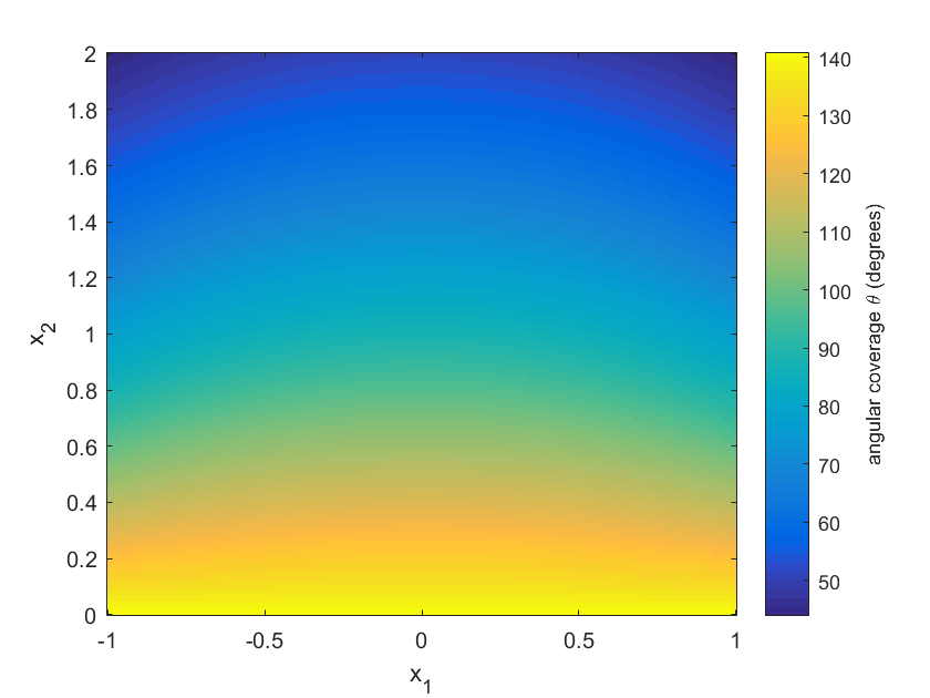
(a) $\theta$ coverage.

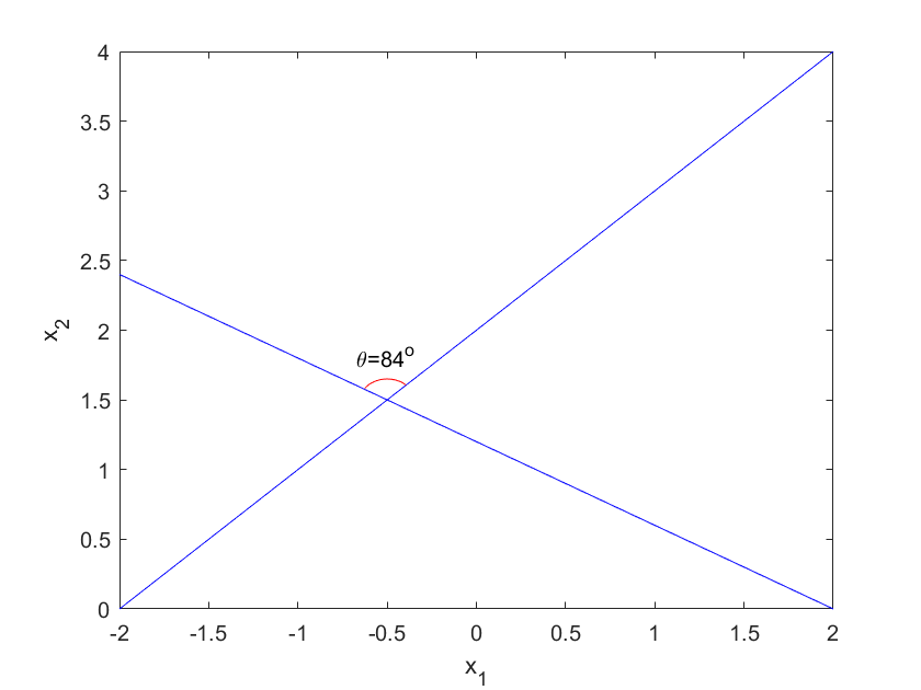
(b) Example $\theta$.

Figure 2. Left – set of angular coverage ($\theta$) with broken-ray data on $[-2,2]\times[0,2]$, for $x_{0}\in[-2,2]$ and $E\in(0,2.83]$ (i.e. when $c=2$, $a=0$ and $b=2.83$). Right – example $\theta$ for the point $(-0.5,1.5)$. The set of directions resolved by the data ($\xi$) is the red cone displayed in the right hand figure, rotated by $90^{\circ}$ about $(-0.5,1.5)$, minus the direction $\xi=(1,0)$.

Note that this theorem does not say anything about singularities of $\mathcal{L}f$ for $({\mathbf{x}},{\boldsymbol{\xi}})\in\mathrm{WF}(f)$ for which $\frac{x_{2}}{q(r)}\in\left\{a,b\right\}$, or $x_{1}-r\omega=\pm c$. Singularities at these wavefront directions are more complicated to analyze and artefacts can be created because of these points. These so-called boundary artefacts are seen in figure 3; the boundary points in the data set labeled “Edge 1” and “Edge 2” in figure 3(a) are points in the support of $R\delta$ at the boundary of the data set, $\mathcal{A}$. Then, you can see the artefacts they create (labeled the same way) in figure 3(c). Similar artefacts are highlighted in the sinogram in figure 3(d) along with the resulting artefacts in figure 3(f). These artefacts are predicted by the microlocal analysis of the operator $\mathcal{L}$, and a more thorough analysis of such artefacts will appear elsewhere.

Proof.

Let $({\mathbf{x}},{\boldsymbol{\xi}})\in\mathrm{WF}^{\alpha}(f)$.

First assume that condition (1) in this theorem holds. Then, by Theorem 3.8,

$$\boldsymbol{\lambda}=(E,\mathbf{x}_{0},-\sigma q(r),-\sigma Eq^{\prime}(r)\boldsymbol{\omega})\in\mathrm{WF}^{\alpha+1/2}(Rf)$$

by (3.24) where $r=g^{-1}\left(\frac{\left|\xi_{1}\right|}{x_{2}\left|\xi_{2}\right|}\right)$ and $\omega=-\frac{\xi_{1}\xi_{2}}{\left|\xi_{1}\xi_{2}\right|}$, $E=\frac{x_{2}}{q(r)}$ and $x_{0}=x_{1}-r\omega$. Since $\frac{\mathrm{d}^{2}}{\mathrm{d}E^{2}}$ is elliptic of order two in this direction, $\boldsymbol{\lambda}\in\mathrm{WF}^{\alpha-3/2}\left(\frac{\mathrm{d}^{2}}{\mathrm{d}E^{2}}Rf\right)$.

If condition (2) of this theorem holds, then $(E,x_{0})\in{\operatorname{int}}(\mathcal{A})$ and since $\chi_{\mathcal{A}}$ is one in a neighborhood of $(E,x_{0})$, $\boldsymbol{\lambda}\in\mathrm{WF}^{\alpha-3/2}\left(\chi_{\mathcal{A}}\frac{\mathrm{d}^{2}}{\mathrm{d}E^{2}}Rf\right)$. Because $R^{*}$ is elliptic of order $-1/2$ and satisfies the semi-global Bolker Assumption, $({\mathbf{x}},\xi)=\mathcal{C}^{t}\circ\left\{\boldsymbol{\lambda}\right\}$ is in $\mathrm{WF}^{\alpha-1}(\mathcal{L}f)$. This statement is proven for $R^{*}$ using the similar arguments to the analogous statement for $R$ at the start of the proof of Theorem 3.8.

Next, if condition (1) of this theorem holds but $\frac{x_{2}}{q(r)}\notin[a,b]$, or $x_{1}-r\omega\notin[-c,c]$, then $(E,x_{0})$ is in the exterior of $\mathcal{A}$ and so $\chi_{\mathcal{A}}\frac{\mathrm{d}^{2}}{\mathrm{d}E^{2}}Rf$ is zero, hence smooth in a neighborhood of $(E,x_{0})$. Since $R^{*}$ is an FIO with canonical relation $\mathcal{C}^{t}$, $({\mathbf{x}},{\boldsymbol{\xi}})=\mathcal{C}^{t}\circ{\boldsymbol{\lambda}}\notin\mathrm{WF}(\mathcal{L}f)$.

Finally, if (1) does not hold then, as discussed in Remark 3.9 $({\mathbf{x}},{\boldsymbol{\xi}})$ does not create any singularity in $Rf$ and therefore not in $\mathcal{L}f$ (i.e., $\mathcal{C}\circ\left\{({\mathbf{x}},{\boldsymbol{\xi}})\right\}=\emptyset$ and so $\mathcal{C}^{t}\circ\mathcal{C}\circ\left\{({\mathbf{x}},{\boldsymbol{\xi}})\right\}=\emptyset$. This finishes the proof. ∎

4. Examples in $\mathbb{R}^{2}$ and reconstructions

In this section we analyze several examples to provide perspective on our results. We present reconstructions by inverse crime (noise level zero) to verify our theory. We note in each case if the conditions of Theorem 3.1 (equivalently Bolker) are satisfied.

Example 4.1 (CST: Bolker satisfied).

Some simple examples of interest are the monomials

(4.1) $$q(r)=r^{\alpha},$$

where $\alpha>0$. In this case $g(r)=\frac{\alpha r^{\alpha-1}}{r^{\alpha}}=\frac{\alpha}{r}$, which is injective on $(0,\infty)$, and $g^{\prime}(r)=-\frac{\alpha}{r^{2}}$, which is never zero. Hence the conditions of Theorem 3.1 are satisfied and the Radon integrals satisfy the Bolker assumption. A specific monomial of interest in X-ray CT and CST is the straight line $q_{C}(r)=r$, when $\alpha=1$. In this case $R_{j}$, for $j=1,2$, reduces to the well known line Radon transform in classical X-ray CT, and $R$ reduces to the broken-ray transforms of [2, 5] in gamma ray source imaging in CST. See figure 1 for example broken-ray integration curves when $x_{0}=3$ and $E=0.5$. Let $B=\{(x,y)\in\mathbb{R}^{2}:x^{2}+(y-1)^{2}<0.2^{2}\}$. Then see figure 3 for reconstructions of a delta function $f=\delta$, centred at $(0,1)$, and disc phantom $f=\chi_{B}$ from $Rf$, when $q=q_{C}$.

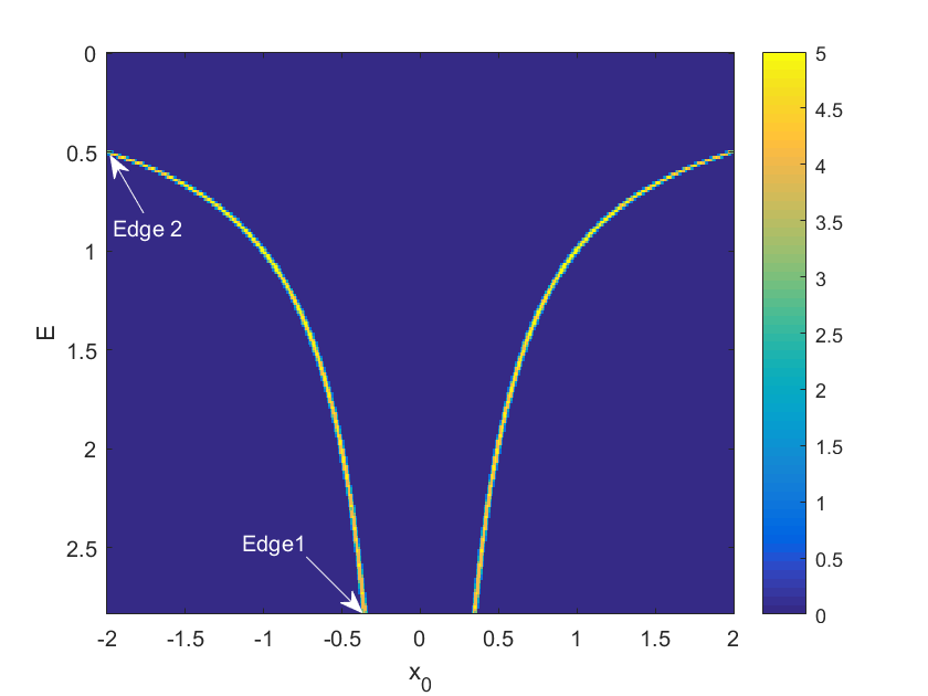
(a) $R\delta$ sinogram.

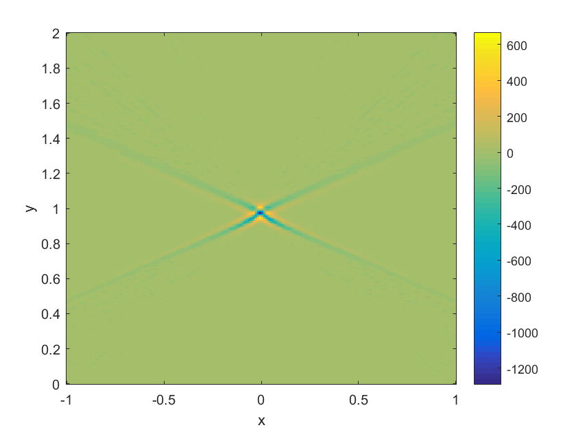
(b) $R^{*}\frac{\mathrm{d}^{2}}{\mathrm{d}E^{2}}R\delta$.

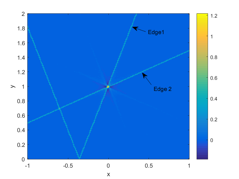
(c) Landweber.

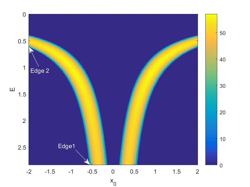
(d) $R\chi_{B}$ sinogram.

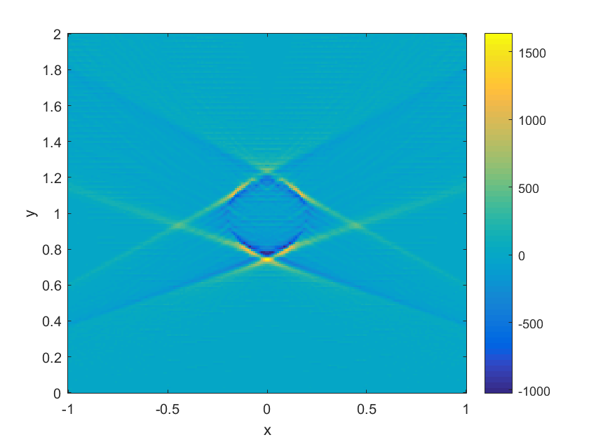
(e) $R^{*}\frac{\mathrm{d}^{2}}{\mathrm{d}E^{2}}R\chi_{B}$.

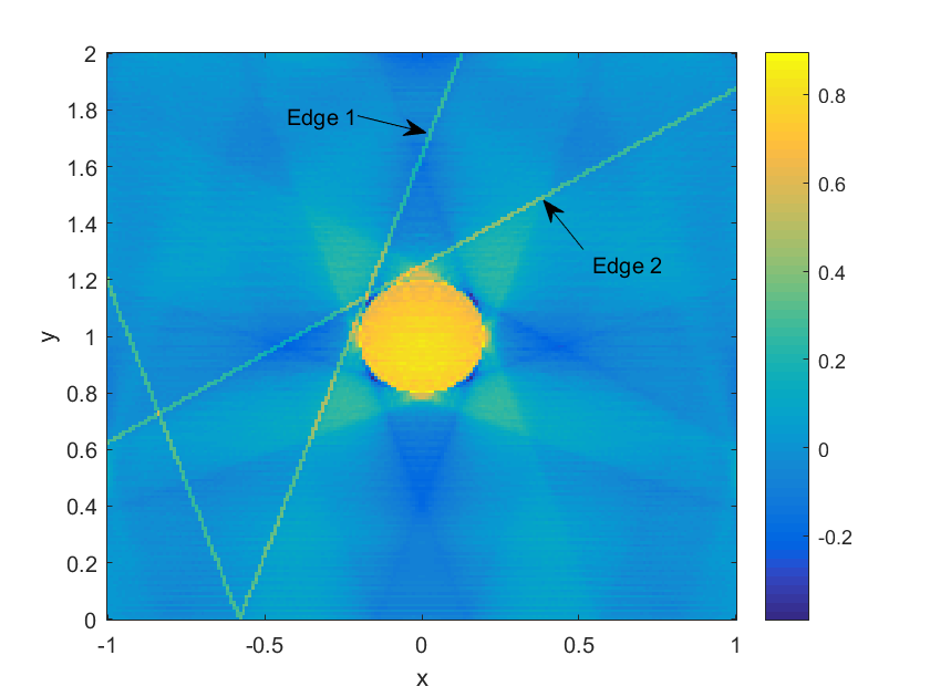
(f) Landweber.

Figure 3. Broken-ray transform reconstructions. Two edges of the data set are highlighted in each case, which correspond to artefacts in the reconstruction. These are highlighted in the Landweber image.

The scanning region used is $[-1,1]\times[0,2]$, and we simulate $Rf(E,x_{0})$ for $E\in(0,2.83)$ and $x_{0}\in[-2,2]$. The delta function is simulated as a characteristic function on a square with small area. That is $\delta\approx\chi_{S}$, where $S=[-0.015,0.015]\times[0.985,1.015]$ (i.e. a $3\times 3$ pixel grid centered on $(0,1)$). The reconstruction methods used are Filtered Back-Projection (FBP) (see figures 3(b) and 3(e) and remark 3.11) using $\frac{\mathrm{d}^{2}}{\mathrm{d}E^{2}}$ as filter, and Landweber iteration (see figures 3(c) and 3(f)). Note the difference in scales of the color bars between figures 3(b) and 3(c), and 3(e) and 3(f). The aim of the generalized Lambda reconstruction (3.27) is to recover the image singularities, and the reconstructed values give primarily qualitative information. Therefore, these color bar ranges of figures 3(b) and 3(e) are chosen to show the singularities of the object. The Landweber iteration approximates the exact solution numerically, and thus the color bar ranges of figures 3(c) and 3(f) more closely represent the original density range (i.e. $[0,1]$ for the phantoms considered).

We see vertical and horizontal blurring due to limited data in the Landweber iteration. This is because not all wavefront directions are visible with broken-ray data, as described by Theorem 3.10. This effect is illustrated in figure 2(a). We can see that there is only limited angular coverage on the boundary of $B$ and at $(0,1)$ (the location of $\delta$), where the test phantoms have singularities. Additionally we see artefacts appearing along broken-rays at the boundary of the dataset. This is due to the sharp cutoff in the sinogram space (see figures 3(a) and 3(d)). We see similar boundary artefacts occurring in [3] in reconstructions from limited line integral data. Two boundary points in the support of $\chi_{A}Rf$ are labelled by “Edge 1” and “Edge 2” in the sinograms of figures 3(a) and 3(d), and they generate artifacts that are shown along broken-ray curves in the image reconstructions of figures 3(c) and 3(f). The broken-ray curves in the image space are labelled similarly by “Edge 1” and “Edge 2”, as in sinogram space. Note that only half of the broken-ray curve at Edge 2 intersects $[-1,1]\times[0,2]$, and hence the Edge 2 artefacts appear along lines in figures 3(c) and 3(f). Similar boundary artefacts are observed in [5], where the authors present reconstructions of $\chi_{B}$ and a Shepp-Logan phantom from $Rf$. The upper $E$ limit used by [5] ($E$ is equivalent to the cone opening angle $\omega$, in the notation of [5]) is greater than the maximum $E$ used here however, and hence the reconstructions [5] better resolve the horizontal singularities.

If artefacts due to a $\Lambda$ (as in Remark 3.3) are present, we would expect to see them highlighted in the FBP reconstruction (as in [39]). This is not the case however and there is no evidence of $\Lambda$ artefacts. This is as predicted by our theory and is in line with the results of [34, Theorem 14] for a related but overdetermined transform which show that the normal operator $R^{*}R$ is a pseudo-differential operator when $q=q_{C}$

Example 4.2 (BST: Bolker satisfied).

The curves of integration in BST are [40]

$$q_{B}(r)=\frac{r}{\sqrt{r^{2}+1}}.$$

See figure 1 for an example Bragg curve when $x_{0}=3$ and $E=2$. $q_{B}$ describes the integration curves for the central scanning profile $x_{2}=0$, using the notation of [40]. Explicitly we set $x_{2}=0$ in [40, equation (4.2)] to obtain $q_{B}$. For an analysis of the general case when $x_{2}\in(-1,1)$, see appendix A.

The first and second order derivatives of $q_{B}$ are

$$q^{\prime}_{B}(r)=\frac{1}{(r^{2}+1)^{\frac{3}{2}}}\neq 0,\ \ \ q^{\prime\prime}_{B}(r)=-\frac{3r}{(r^{2}+1)^{\frac{5}{2}}}.$$

Hence $g_{B}(r)=\frac{q^{\prime}(r)}{q(r)}=\frac{1}{r(r^{2}+1)}$, which is injective on $(0,\infty)$, and it follows that

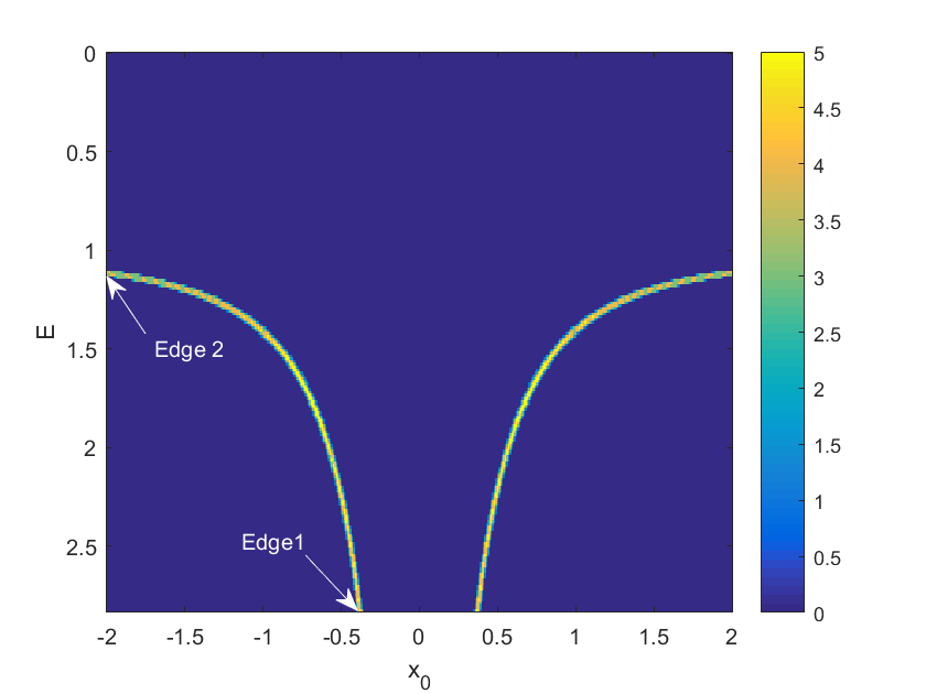
(a) $R\delta$ sinogram.

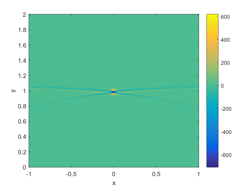
(b) $R^{*}\frac{\mathrm{d}^{2}}{\mathrm{d}E^{2}}R\delta$.

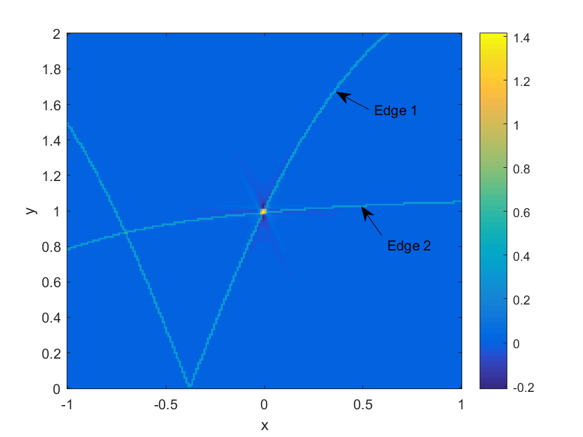
(c) Landweber.

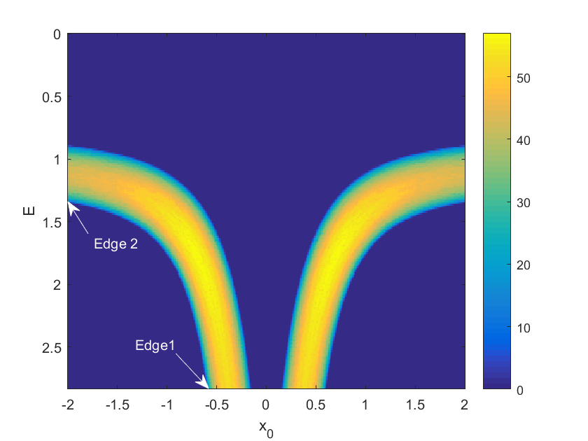
(d) $R\chi_{B}$ sinogram.

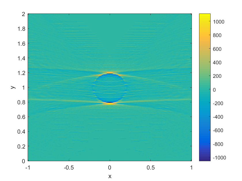
(e) $R^{*}\frac{\mathrm{d}^{2}}{\mathrm{d}E^{2}}R\chi_{B}$.

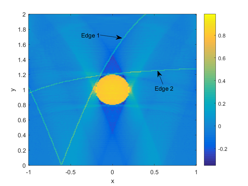
(f) Landweber.

Figure 4. Bragg transform reconstructions. Two edges of the data set are highlighted in each case, which correspond to artefacts in the reconstruction. These are highlighted in the Landweber image.

$$g^{\prime}_{B}(r)=\frac{q^{\prime\prime}(r)}{q(r)}-\frac{q^{\prime}(r)^{2}}{q^{2}(r)}=-\frac{3r^{2}+1}{r^{2}(r^{2}+1)^{2}}<0.$$

Thus the Bolker assumption holds for $R_{j}$ and $R$ when $q=q_{B}$ in BST. See figure 4 for reconstructions of $f=\delta$ and $f=\chi_{B}$ from $Rf$, when $q=q_{B}$. The scanning region is $[-1,1]\times[0,2]$ and $Rf$ is simulated for $E\in(0,2.83)$ and $x_{0}\in[-2,2]$, as in example 4.1. We see artefacts appearing along Bragg curves at the boundary of the dataset, due to the cutoff in sinogram space. The points on the sinograms in figures 4(a) and 4(d) labeled “Edge 1” and “Edge 2” are in the support of the data and on the boundary of the data set; the sharp cutoff at the boundary creates artifacts as highlighted along Bragg curves (which are labeled “Edge 1” and “Edge 2” in figures 4(c) and 4(f)). Similar to example 4.1, only half of the Bragg curve at Edge 2 intersects $[-1,1]\times[0,2]$, and hence the Edge 2 artefacts appear along one-sided Bragg curves (minus the reflected curve in $x=x_{0}$) in figures 3(c) and 3(f). There is a horizontal and vertical blurring due to limited data in the Landweber reconstruction. This observation is in line with the theory of section 3.3 and Theorem 3.10. We noticed a similar effect in reconstructions from broken-ray curves, when $q=q_{C}$ in example 4.1. In this case the vertical blurring is less pronounced. The vertical singularities appear sharper in the FBP reconstructions also. This is because of the flatter gradients of the Bragg curves as $r\to\infty$, compared to straight lines, which allow the Bragg curves to better detect vertical singularities. That is the Bragg curves are such that

$$0=\lim_{r\to\infty}q^{\prime}_{B}(r)<\min\left(\{q^{\prime}_{C}(r):r\in[0,\infty)\}\right)=1.$$

See figure 5 for a visualization. We display a shifted Bragg curve $q_{B}$ and Compton curve $q_{C}$. $q_{B}$ and $q_{C}$ intersect on the boundary of $\chi_{B}$ at $(0,1.2)$, where a singularity occurs in the direction $(0,1)$ (a vertical singularity). The gradients at $(0,1.2)$ are, $q^{\prime}_{C}(0)=1.2$ and $q^{\prime}_{B}(0)\approx 0.6$, approximately half the gradient of $q_{C}$ at $(0,1.2)$. The reduction in gradient allows for better detection of the singularity at $(0,1.2)$ using Bragg curves.

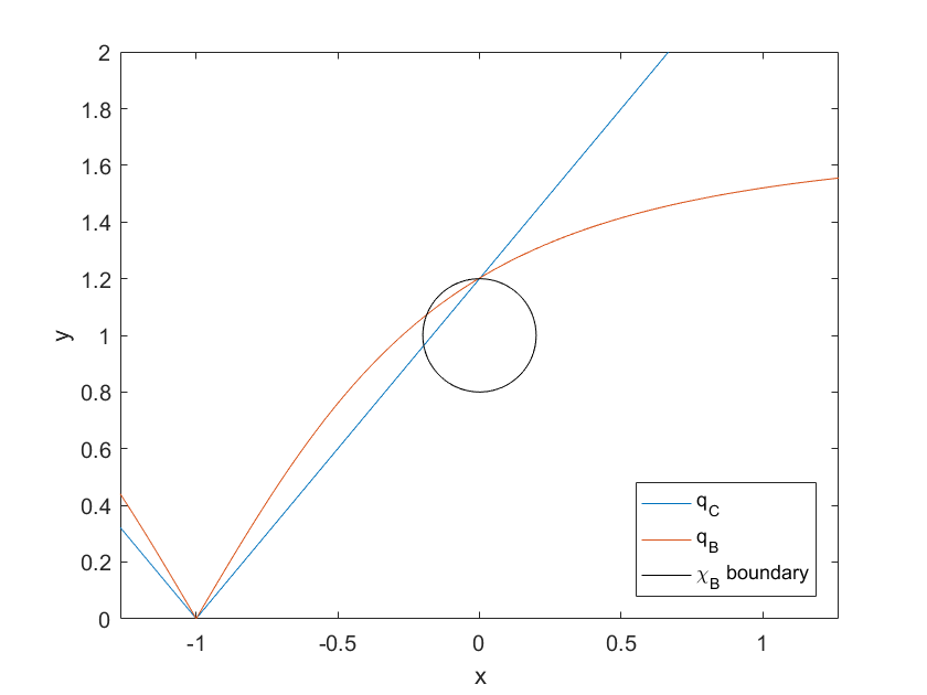
Figure 5. Illustration of Compton vs Bragg, vertical edge detection.

Example 4.3 (sinusoidal curves: Bolker not satisfied).

Here we give an example $q$ which satisfies (3.1), but fails to satisfy the Bolker assumption. We define the sinusoidal curves as

(4.2) $$q_{S}(r)=(1+\epsilon)r+\sin r,$$

where $\epsilon>0$. See figure 6(a). We can check that $q_{S}(0)=0$ and $q^{\prime}_{S}(r)=(1+\epsilon)+\cos r>\epsilon>0$, and hence (3.1) is satisfied. As (3.1) holds, it follows that $R$ is injective by [40, Theorem 5.2], and hence there are no artefacts due to null space. We have

$$g_{S}(r)=\frac{(1+\epsilon)+\cos r}{(1+\epsilon)r+\sin r},$$

which is non-injective. See figure 6(b). Further $g^{\prime}_{S}(r)=\frac{g_{1}(r)}{q^{2}_{S}(r)}$, where

$$g_{1}(r)=(1+\epsilon)\left(r\sin r+2\cos r\right)+(1+\epsilon)^{2}+1,$$

and hence $g^{\prime}_{S}(r)=0\iff g_{1}(r)=0$, for $r\in(0,\infty)$. $g_{1}$ is zero for infinitely many $r\in\mathbb{R}$, for any $\epsilon$ chosen. See figure 6(c).

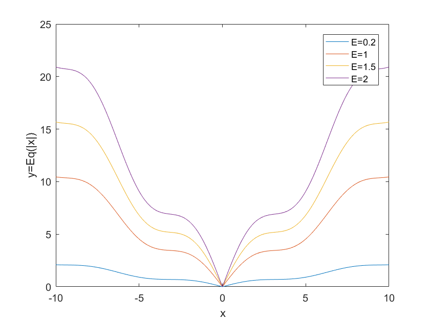
(a) $Eq_{S}$ for $E\in\{0.2,1,1.5,2\}$.

(b) $g_{S}$.

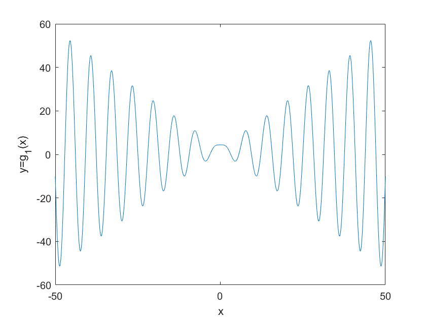
(c) $g_{1}$.

Figure 6. The curves $q_{S}$, $g_{S}$ and $g_{1}$, for $\epsilon=0.1$. Note that the $x$ and $y$ axis limits vary across sub-figures (A), (B) and (C).

Hence for the sinusoidal curves the Bolker assumption is not satisfied, and we can expect to see artefacts due to $\Lambda$ (see Remark 3.3) in the reconstruction. We note that $R$ and the $R_{j}$ are injective by [40, Theorem 5.2] and hence we expect no additional artefacts due to null space. The scanning region used in this example is $[-10,10]\times[0,20]$, and $Rf$ is simulated for $E\in(0,3.77)$ and $x_{0}\in[-20,20]$. We scale up by a factor of $10$ in this case to allow for multiple oscillations of the sinusoidal curves within the scanning region. See figure 6(a). On $[-1,1]\times[0,2]$ (the scanning region used in examples 4.1 and 4.2), the $q_{S}$ curves are appear approximately as broken-rays (V-lines) in the simulations, since $\sin r\approx r$ for $r$ close to zero. Hence we scale the scanning region size by 10 here to better highlight the discrepancies between broken-ray and sinusoidal transform reconstruction. In these dimensions the $x_{0}$ range used is the same (relatively speaking) as in examples 4.1 and 4.2. The energy range is chosen so that the integration curves have a wide variety of gradients, and sufficiently cover $[-10,10]\times[0,20]$.

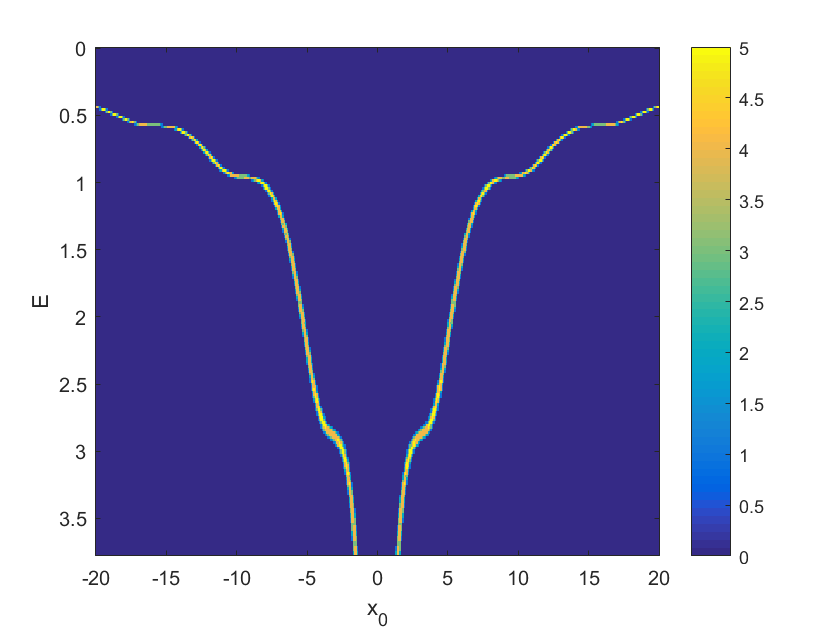
(a) $R\delta$ sinogram.

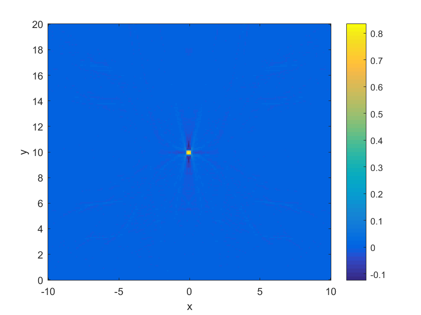
(b) Landweber.

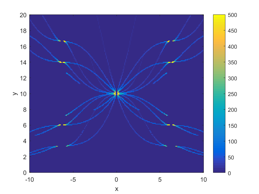
(c) $\Lambda$ artefacts.

(d) $R^{*}\frac{\mathrm{d}^{2}}{\mathrm{d}E^{2}}R\delta$.

Figure 7. Sinusoid transform reconstructions of $f=\delta$.

See figure 7 for reconstructions of $f=\delta$, centered at $(0,10)$, from $Rf$, when $q=q_{S}$. As predicted, we see artefacts appearing in the reconstructions on the sinusoidal curves which intersect $f$ normal to a singularity (equivalently, any curve which intersects $f=\delta$). As described in Remark 3.3, we use $g_{S}$ to map the singularities of $\delta$ (at $(0,10)$, in all directions) to artefacts along sinusoidal curves. The artefacts predicted by $g_{S}$ and our theory are shown in figure 7(c). The same artefacts are observed in the FBP reconstruction in figure 7(d), and align exactly with our predictions. Note that we have removed the reconstructed delta function from figure 7(d) (i.e. we set the central three image columns to zero) and truncated the color bars, to better show the artefacts. The artefacts are also observed faintly in the Landweber reconstruction in figure 7(b). This is in line with the theory of [39], where the microlocal artefacts are shown to be highlighted in FBP reconstructions.

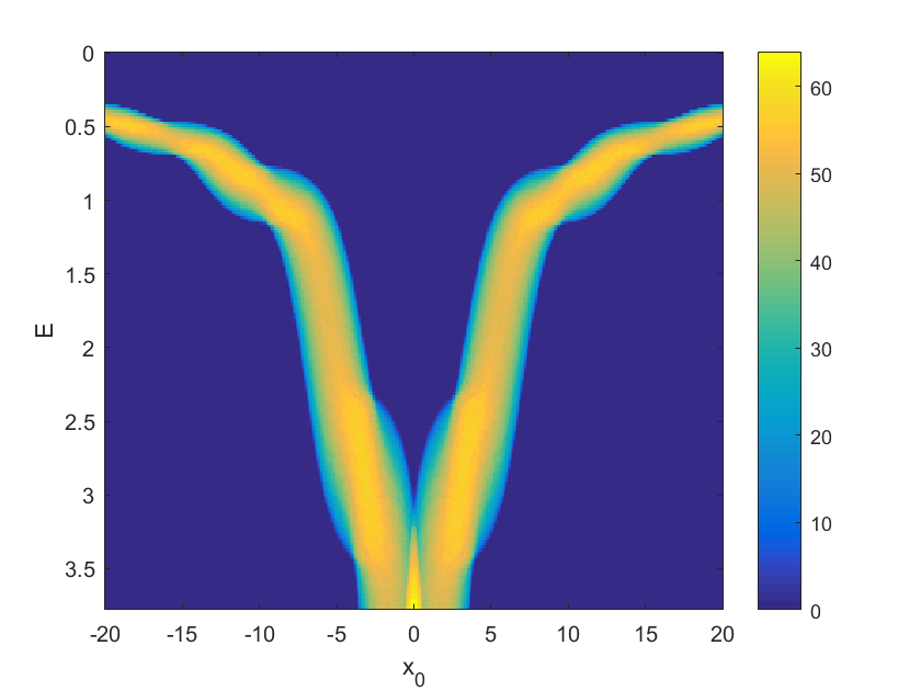
(a) $R\chi_{B}$ sinogram.

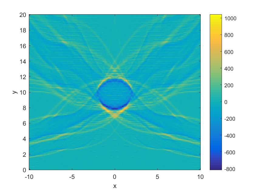
(b) $R^{*}\frac{\mathrm{d}^{2}}{\mathrm{d}E^{2}}R\chi_{B}$.

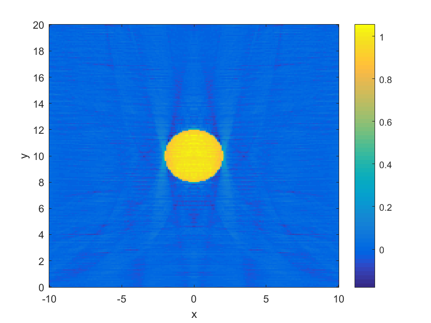
(c) Landweber.

Figure 8. Sinusoid transform reconstructions of $f=\chi_{B}$.

Let $B=\{(x,y)\in\mathbb{R}^{2}:x^{2}+(y-10)^{2}<4\}$. See figure 8 for reconstructions of $f=\chi_{B}$ from $Rf$. Similar to the $f=\delta$ case, we see artefacts appearing on the sinusoidal curves which are tangent to the boundary of $\chi_{B}$ (i.e. the set of points where $f$ has singularities). See figure 8(b). Further $q_{S}$ has a larger range of gradients, when compared to $q_{C}$ and $q_{B}$. That is $\mu\left(q^{\prime}_{S}([0,\infty))\right)>\mu\left(q^{\prime}_{C}([0,\infty))\right),\mu\left(q^{\prime}_{B}([0,\infty))\right)$, where $\mu$ is Lebesgue measure. Hence the Radon data can resolve the image singularities in more directions with sinusoidal curves, when compared to BST and CST curves. See figure 5 and the arguments towards the end of example 4.2. Due to the increased range of gradients, the horizontal and vertical blurring effects observed in examples 4.1 and 4.2 are less prominent here. This is evidenced by figure 8(c).

5. Conclusions and further work

Here we have presented a novel microlocal analysis of a generalized cone Radon transform $R$, which defines the integrals of $f\in L^{2}_{c}(\mathbb{R}^{n-1}\times(0,\infty))$ over the $(n-1)$-dimensional surfaces of revolution of smooth curves $q$. We proved that $R$ is an elliptic FIO order $\frac{1-n}{2}$, and we gave an explicit expression for the left projection $\Pi_{L}$. Our main theorem (Theorem 3.1) shows that $\Pi_{L}$ satisfies the semi-global Bolker assumption if and only if $g=q^{\prime}/q$ is an immersion. Two main applications of this theory are in Compton camera imaging in CST, and crystalline structure imaging in BST and airport baggage screening. In section 4 we showed that the CST and BST integration curves satisfied the conditions of Theorem 3.1, thus proving that the CST and BST Radon FIO satisfy the Bolker assumption. Additionally we gave example “sinusoidal” $q$ in example 4.3 for which the corresponding Radon transforms violate the Bolker assumption, and we provided simulated image reconstructions from sinusoidal Radon data. We saw artefacts appearing along the sinusoidal curves which intersected the singularities of $f$ normal to the direction of the singularity. The artefacts observed in reconstruction were shown to align exactly with our predictions and the results of Theorem 3.1.

The theory presented here explains some key microlocal properties of a range of Radon transformations in $\mathbb{R}^{n}$, whereby the integrals are taken over generalized cones with vertex constrained to the ${\mathbf{x}}^{\prime}=(x_{1},\ldots,x_{n-1})$ plane. In further work we aim to generalize the set of cone vertices to suit a wider range of imaging geometries. For example, we could consider the vertex sets which are smooth $n-1$ manifolds in $\mathbb{R}^{n}$, in a similar vein to [41] in $\mathbb{R}^{3}$.

It is noted that quality of reconstruction (with zero noise), from CST and BST data, is low using the methods considered, and there are significant boundary artefacts in the reconstructions presented (see examples 4.1 and 4.2). The reconstruction methods used here were chosen to highlight the image artefacts predicted by our theory, so this is as expected. In future work we aim to derive practical reconstruction algorithms and regularization penalties to combat the artefacts, for example using smoothing filters as in [5, 12, 3] to remove boundary artefacts. An algebraic approach may also prove fruitful (as is discovered in [38] for CST artefacts), as this would allow us to apply the powerful regularization methods from the discrete inverse problems literature, e.g. Total Variation (TV).

Appendix A Bragg curve analysis for $x_{2}\in(-1,1)$

Throughout this section we will use the notation of [40], where $x_{2}\in(-1,1)$ now describes the coordinates of the scanned line profile in BST (i.e., the vertex of the V is at the point $(x_{1},x_{2})$, see [40, figure 1]); $x_{1}\in\mathbb{R}$ plays the same role in both articles.

In [40] the authors consider a one-dimensional set of 2-D Radon transforms, with imaging applications in BST and spectroscopy. In example 4.2 we considered the curves of integration defined by $q_{B}(x_{1})=\frac{x_{1}}{\sqrt{x_{1}^{2}+1}}$. These curves describe a special case of the Radon transforms of [40], where the scanned line profile is on the centerline of the imaging apparatus, $x_{2}=0$. Here we consider the general $x_{2}\in(-1,1)$ case. The full set of integration curves in BST are described by [40, equation (4.2)]:

(A.1) $$q_{B}(x_{1},x_{2})=\frac{1}{\sqrt{2}}\sqrt{1+\frac{x_{1}^{2}-(1-x_{2}^{2})}{\sqrt{x_{1}^{2}+(x_{2}+1)^{2}}\sqrt{x_{1}^{2}+(1-x_{2})^{2}}}}.$$

Note that $q_{B}(x_{1},0)=\frac{x_{1}}{\sqrt{x_{1}^{2}+1}}$. In [40] the 1-D set of Radon transforms considered take integrals over the broken-ray curves $q_{B}(\cdot,x_{2})$ for each $x_{2}\in(-1,1)$. The broken-ray integrals are described by the generalized cone transform of (3.7) with $q=q_{B}(\cdot,x_{2})$. Note that $q_{B}(\cdot,x_{2})>0$ for $x_{1}>0$, for every $x_{2}\in(-1,1)$, so 3.1 is satisfied. Here we aim to show that $h_{B}(\cdot,x_{2})=\frac{1}{g_{B}(\cdot,x_{2})}=\frac{q_{B}(\cdot,x_{2})}{q^{\prime}_{B}(\cdot,x_{2})}$ is an immersion for each $x_{2}\in(-1,1)$, thus showing that the Bolker assumption is satisfied for every scanning profile considered. As the calculation of the second order derivatives of $q_{B}$ in $x_{1}$ is cumbersome, we verify Bolker numerically, for some chosen range of $x_{1},x_{2}$. Note that we consider the reciprocal $h_{B}$ of $g_{B}$ here to avoid division by values close to zero as $x_{1}\to 0$, and since $g^{\prime}_{B}(\cdot,x_{2})=0\iff h^{\prime}_{B}(\cdot,x_{2})=0$ for $g_{B}(\cdot,x_{2}):(0,\infty)\to(0,\infty)$.

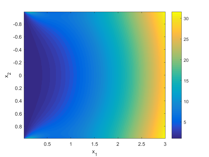
(a) $h^{\prime}_{B}(x_{1},x_{2})$. $\min_{(0,3]\times(-1,1)}(h^{\prime}_{B})\approx 1$.

Figure 9. Numerical validation of $h^{\prime}_{B}(\cdot,x_{2})\neq 0$ for each $x_{2}\in(-1,1)$.

We choose to simulate $h^{\prime}_{B}$ for $x_{1}\in(0,3]$ and $x_{2}\in(-1,1)$. The maximum $x_{1}$ (i.e. $x_{1}=3$) chosen is the maximum $x_{1}$ considered in the scanning setup of example 4.2. That is with scanning region $[-1,1]\times[0,2]$ and $x_{0}\in[-2,2]$ (the maximum $x_{1}$ occurs when $x_{0}=-2,2$ at the edge of the scanning region). We need only consider positive $x_{1}$ since $q_{B}$ of equation (A.1) is symmetric in $x_{1}$ about $x_{1}=0$. See figure 9, where we display $h^{\prime}_{B}$ on $(0,3]\times(-1,1)$. Finite differences are used to approximate the derivatives. The minimum value of $h^{\prime}_{B}$ in this range is $\min_{(0,3]\times(-1,1)}(h^{\prime}_{B})\approx 1$, which indicates that the Bolker assumption is satisfied in the scanning geometry of example 4.2.

References

- [1] G. Ambartsoumian. Inversion of the V-line Radon transform in a disc and its applications in imaging. Computers & Mathematics with Applications, 64(3):260–265, 2012.
- [2] G. Ambartsoumian and M. J. Latifi Jebelli. The V-line transform with some generalizations and cone differentiation. Inverse Problems, 35(3):034003, 29, 2019.
- [3] L. Borg, J. Frikel, J. S. Jørgensen, and E. T. Quinto. Analyzing reconstruction artifacts from arbitrary incomplete X-ray CT data. SIAM Journal on Imaging Sciences, 11(4):2786–2814, 2018.
- [4] J. Cebeiro, M. Morvidone, and M. Nguyen. Back-projection inversion of a conical Radon transform. Inverse Problems in Science and Engineering, 24(2):328–352, 2016.
- [5] J. Cebeiro, M. A. Morvidone, and M. K. Nguyen. The Radon transform on V-lines: Artifact analysis and image enhancement. In XVII Workshop on Information Processing and Control (RPIC), pages 1–6. IEEE, 2017.
- [6] A. M. Cormack. Radon’s problem for some surfaces in . Proc. Amer. Math. Soc., 99(2):305–312, 1987.
- [7] J. J. Duistermaat. Fourier integral operators, volume 130 of Progress in Mathematics. Birkhäuser, Inc., Boston, MA, 1996.
- [8] J. J. Duistermaat and L. Hormander. Fourier integral operators, volume 2. Springer, 1996.
- [9] L. Florescu, V. A. Markel, and J. C. Schotland. Single-scattering optical tomography: simultaneous reconstruction of scattering and absorption. Physical Review E, 81(1):016602, 2010.
- [10] L. Florescu, V. A. Markel, and J. C. Schotland. Inversion formulas for the broken-ray Radon transform. Inverse Problems, 27(2):025002, 2011.
- [11] L. Florescu, J. C. Schotland, and V. A. Markel. Single-scattering optical tomography. Physical Review E, 79(3):036607, 2009.
- [12] J. Frikel and E. T. Quinto. Artifacts in incomplete data tomography with applications to photoacoustic tomography and sonar. SIAM J. Appl. Math., 75(2):703–725, 2015.
- [13] R. Gouia-Zarrad and G. Ambartsoumian. Exact inversion of the conical Radon transform with a fixed opening angle. Inverse Problems, 30(4):045007, 12, 2014.
- [14] V. Guillemin and S. Sternberg. Geometric Asymptotics. American Mathematical Society, Providence, RI, 1977.
- [15] M. Haltmeier. Exact reconstruction formulas for a Radon transform over cones. Inverse Problems, 30(3):035001, 2014.
- [16] L. Hörmander. Fourier Integral Operators, I. Acta Mathematica, 127:79–183, 1971.
- [17] L. Hörmander. The analysis of linear partial differential operators. I. Classics in Mathematics. Springer-Verlag, Berlin, 2003. Distribution theory and Fourier analysis, Reprint of the second (1990) edition [Springer, Berlin].
- [18] L. Hörmander. The analysis of linear partial differential operators. III. Classics in Mathematics. Springer, Berlin, 2007. Pseudo-differential operators, Reprint of the 1994 edition.
- [19] L. Hörmander. The analysis of linear partial differential operators. IV. Classics in Mathematics. Springer-Verlag, Berlin, 2009. Fourier integral operators, Reprint of the 1994 edition.
- [20] C.-Y. Jung and S. Moon. Inversion formulas for cone transforms arising in application of Compton cameras. Inverse Problems, 31(1):015006, 2015.
- [21] P. Kuchment and F. Terzioglu. Three-dimensional image reconstruction from Compton camera data. SIAM Journal on Imaging Sciences, 9(4):1708–1725, 2016.
- [22] Á. Kurusa. Support curves of invertible Radon transforms. Arch. Math. (Basel), 61(5):448–458, 1993.
- [23] V. Maxim, M. Frandeş, and R. Prost. Analytical inversion of the Compton transform using the full set of available projections. Inverse Problems, 25(9):095001, 2009.
- [24] S. Moon. On the determination of a function from its conical radon transform with a fixed central axis. SIAM Journal on Mathematical Analysis, 48(3):1833–1847, 2016.
- [25] S. Moon. Inversion of the conical Radon transform with vertices on a surface of revolution arising in an application of a compton camera. Inverse Problems, 33(6):065002, 2017.
- [26] S. Moon and M. Haltmeier. Analytic inversion of a conical radon transform arising in application of Compton cameras on the cylinder. SIAM Journal on imaging sciences, 10(2):535–557, 2017.
- [27] M. Morvidone, M. K. Nguyen, T. T. Truong, and H. Zaidi. On the V-line Radon transform and its imaging applications. International Journal of Biomedical Imaging, 2010, 2010.
- [28] M. K. Nguyen, T. T. Truong, and P. Grangeat. Radon transforms on a class of cones with fixed axis direction. Journal of Physics A: Mathematical and General, 38(37):8003, 2005.
- [29] V. P. Palamodov. A uniform reconstruction formula in integral geometry. Inverse Problems, 28(6):065014, 2012.
- [30] B. E. Petersen. Introduction to the Fourier transform & pseudodifferential operators, volume 19 of Monographs and Studies in Mathematics. Pitman (Advanced Publishing Program), Boston, MA, 1983.
- [31] E. T. Quinto. The dependence of the generalized Radon transform on defining measures. Trans. Amer. Math. Soc., 257:331–346, 1980.
- [32] E. T. Quinto. Singularities of the X-ray transform and limited data tomography in and . SIAM J. Math. Anal., 24:1215–1225, 1993.
- [33] W. Rudin. Functional analysis. McGraw-Hill Book Co., New York, 1973. McGraw-Hill Series in Higher Mathematics.
- [34] F. Terzioglu. Some analytic properties of the cone transform. Inverse Problems, 35:034002, 2019.
- [35] F. Terzioglu, P. Kuchment, and L. Kunyansky. Compton camera imaging and the cone transform: a brief overview. Inverse Problems, 34(5):054002, 16, 2018.
- [36] T. T. Truong and M. K. Nguyen. New properties of the V-line Radon transform and their imaging applications. Journal of Physics A: Mathematical and Theoretical, 48(40):405204, 2015.
- [37] T. T. Truong, M. K. Nguyen, and H. Zaidi. The mathematical foundations of 3D Compton scatter emission imaging. International journal of biomedical imaging, 2007, 2007.
- [38] J. Webber and E. T. Quinto. Microlocal analysis of a Compton tomography problem. SIAM Journal on Imaging Science, 2020. to appear.
- [39] J. Webber, E. T. Quinto, and E. L. Miller. A joint reconstruction and lambda tomography regularization technique for energy-resolved X-ray imaging. Inverse Problems, 2020. to appear.
- [40] J. W. Webber and E. L. Miller. Bragg scattering tomography. arXiv preprint arXiv:2004.10961, 2020.
- [41] Y. Zhang. Recovery of singularities for the weighted cone transform appearing in Compton camera imaging. Inverse Problems, 36(2):025014, 2020.