Evading Anderson localization in a one-dimensional conductor with correlated disorder

Abstract

We show that a one dimensional disordered conductor with correlated disorder has an extended state and a Landauer resistance that is non-zero in the limit of infinite system size in contrast to the predictions of the scaling theory of Anderson localization. The delocalization transition is not related to any underlying symmetry of the model such as particle-hole symmetry. For a wire of finite length the effect manifests as a sharp transmission resonance that narrows as the length of the wire is increased. Experimental realizations and applications are discussed including the possibility of constructing a narrow band light filter.

I Introduction

In a seminal paper in 1958 Anderson demonstrated that electronic states in disordered solids may be localized over a range of energies anderson . Over the next two decades, studies of disordered electronic systems culminated in the discovery that in one and two dimensions electronic states are always localized, no matter how weak the disorder, while in three dimensions localized and extended states can exist over different ranges of energy, separated by a mobility edge gangone . These findings completely subverted the simple dogma of band theory, showing that for weakly interacting electrons, disorder—rather than the band structure in the clean limit—determined whether a material is a conductor or insulator at low temperature, and that at low temperature all weakly interacting materials are insulators in one and two dimensions leer . Moreover the ideas of Anderson localization proved relevant to optics, acoustics, cold atoms, neural networks, medical imaging and in general to any problem of coherent propagation of waves in a random medium fifty .

In the case of one dimension in particular it has been possible to derive exact results and even rigorous proofs of localization for appropriate models ishii gangtwo . Two distinct approaches have been developed to describe the universal features of localization. The first approach, grounded in random matrix theory, posits that the distribution of transfer matrices in one dimension undergoes diffusion in the space of possible transfer matrices as a function of the length of the conductor mello . This approach, which is restricted to one dimension, reveals that the conductance has a broad log normal distribution, with very different typical and mean values, both of which decay exponentially with the length of the system (a highly non-Ohmic size dependence). Field theory methods, based on replicas stone or supersymmetry efetov for disorder averaging, likewise describe the universal features of localization on length scales that are large compared to the microscopic elastic scattering length, and confirm the picture described above. Thus localization, particularly in one dimension, is now a well-established paradigm.

One known exception to complete localization in one dimension is systems with particle-hole symmetry balents . In this case it is known that at the symmetric point of zero energy there is an extended state and hence a delocalization transition that separates Anderson insulators above and below zero energy. More generally the discovery that quantum systems can be classified into ten symmetry classes zirnbauer based on the absence or presence of particle-hole and time-reversal symmetries has furnished additional examples of delocalization at zero energy ilya . Another example of an extended state at an isolated energy is provided by the quantum dimer model philip . In this case the delocalization happens because the individual scatterers become transparent at a common resonant energy making the system effectively clean at that energy. Other than that every attempt to identify extended states (e.g. numerically) has foundered, strengthening the belief in the inevitability of localization in one dimension.

Nonetheless in this paper we report the astonishing finding that for a model of correlated disorder also it is possible to for the system to undergo delocalization. The extended states we find do not depend upon the perfect transparency of individual impurities or on any underlying symmetries of the model but rather upon local correlations amongst successive scatterers. The model consists of symmetric scatterers that are separated by variable distances. Both the opacity of the individual scatterers and the spacing between them are random variables. However there are correlations amongst these random variables: the spacing between the successive scatterers is constrained by the opacities of the scatterers.

The remainder of the paper is organized as follows. In section II we introduce the model and show that it can be obtained from an underlying tight binding model with on-site disorder. In section III we demonstrate using a combination of analytic arguments and numerical simulations that the probability of non-zero conductance remains finite no matter how long the conductor grows contrary to the localization paradigm. In section IV we offer some concluding remarks on possible experimental tests, applications and open questions.

II The Model

II.1 Individual scatterers

To be concrete, we consider a one-dimensional lattice with non-interacting electrons and nearest neighbor hopping. The potential at each site is either zero or is a random number between $-W$ and $W.$ The corresponding Schrödinger equation is the difference equation

$$\psi_{n-1}+V_{n}\psi_{n}+\psi_{n+1}=E\psi_{n}.$$ (1)

Here $\psi_{n}$ is the wavefunction at site $n$ and $V_{n}$ is the site potential. Note that in the absence of disorder ($V_{n}=0$ for all $n$) the solutions are plane waves $\psi_{n}=\exp(ikn)$ with energy $E=2\cos k$. Sites where $V_{n}\neq 0$ are called scatterers, and we constrain the system so that two scatterers cannot be adjacent to each other. Thus the system can be understood as a sequence of scatterers, with each successive pair of scatterers separated by a lattice segment where $V=0,$ i.e. a clean segment. Our strategy is to find the $S$-matrix for each scatterer, and combine them appropriately.

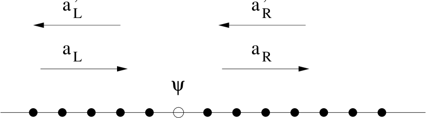
Figure 1: A scattering site, with incoming and outgoing waves on both sides. The wavefunction at the scattering site is $\psi.$ The phases of the waves on both sides are chosen so that the amplitude would have been $a_{L,R}+a^{\prime}_{L,R}$ at the scattering site if the waves from the left/right were to continue uninterrupted through the scattering site.

Figure 1 shows a single scatterer. We make the ansatz

$$\psi_{n} = a_{L}\exp(ikn)+a^{\prime}_{L}\exp(-ikn)\hskip 5.69054pt{\rm for}\hskip 5.69054ptn\leq 0$$ (2)

$$= a_{R}\exp(ikn)+a^{\prime}_{R}\exp(-ikn)\hskip 5.69054pt{\rm for}\hskip 5.69054ptn\geq 0$$

Making use of the Schrödinger Eq. (1) for $n=0$ we obtain

$$a_{L}+a^{\prime}_{L} = \psi$$

$$a_{R}+a^{\prime}_{R} = \psi$$

$$(2\cos k-V)\psi = a_{L}e^{-ik}+a^{\prime}_{L}e^{ik}+a_{R}e^{ik}+a^{\prime}_{R}e^{-ik}.$$ (3)

Solving eq (3) yields

$$\begin{pmatrix}a^{\prime}_{L}\\ a_{R}\end{pmatrix}=S\begin{pmatrix}a_{L}\\ a^{\prime}_{R}\end{pmatrix}$$ (4)

Here the $2\times 2$ $S$-matrix connects the outgoing amplitudes to the incoming amplitudes. Explicitly, we find

$$S(V,k)=-\frac{1}{2i\sin k+V}\begin{pmatrix}V&-2i\sin k\\ -2i\sin k&V\end{pmatrix}.$$ (5)

The form of the $S$-matrix for a single scatterer is powerfully constrained by general principles. Probability conservation imposes unitarity, $S^{\dagger}S=1$. Parity imposes the additional requirements that $S_{11}=S_{22}$ and $S_{12}=S_{21}$. The most general $2\times 2$ matrix consistent with these requirements may be parametrized as

$$S=e^{i\gamma}\begin{pmatrix}\cos\theta&i\sin\theta\\ i\sin\theta&\cos\theta.\end{pmatrix}$$ (6)

where $0\leq\theta\leq\pi/2$ and $0\leq\gamma<2\pi$. It follows from Eqs. (4) and (6) that the transmission coefficient is $\sin^{2}\theta$ and the reflection coefficient is $\cos^{2}\theta$. Hence we refer to the parameter $\theta$ as the opacity of the $S$-matrix.

Comparison of Eqs. (5) and (6) shows that for the tight binding model analyzed above the opacity $\theta$ and the overall phase $\gamma$ for a single scatterer are given by

$$\exp(i\theta) = \pm\frac{V-2i\sin k}{\sqrt{V^{2}+4\sin^{2}k}}$$

$$\exp(i\gamma) = \mp\frac{\sqrt{V^{2}+4\sin^{2}k}}{V+2i\sin k}=-\exp(i\theta)$$ (7)

where the sign on the right hand side is positive (negative) when $V$ is positive (negative), i.e. $\cos\theta>0.$ The fact that $\theta$ and $\gamma$ are related for this model is not true in general. This coincidence will play no role in our subsequent analysis.

II.2 Combining scatterers

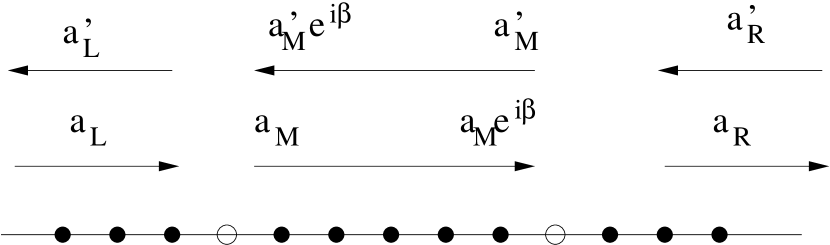
Figure 2: Two scatterers, with waves propagating to the left and to the right in each region. In the middle region, the left-moving wave is incoming for the first scatterer and outgoing for the second scatterer, and vice-versa for the second scatterer. The amplitudes of both of these are defined to be zero at the scatterer they start from, and $\exp[ik(L+1)]=\exp[i\beta]$ at the scatterer they end up at, where $k$ is the wavevector and $L$ is the length of the region between the scatterers; in the figure, $L=5.$

The complete lattice can be treated as a sequence of scatterers, separated by free propagation segments of variable length. Since the lattice is not left-right symmetric, the $S$-matrix of the entire system is not as constrained as Eq.(6). Nevertheless, time reversal invariance requires that $S^{*}=S^{-1}$ which, together with the unitarity of $S,$ implies that $S=S^{T}.$ Therefore we obtain the parameterization

$$S_{N}=e^{i\gamma_{N}}\begin{pmatrix}\cos\theta_{N}e^{i\delta_{N}}&i\sin\theta_{N}\\ i\sin\theta_{N}&\cos\theta_{N}e^{-i\delta_{N}}\end{pmatrix}$$ (8)

where $S_{N}$ is the $S$-matrix of a lattice with $N$ scatterers and the parameters have the domain $0\leq\theta_{N}\leq\pi/2$, $0\leq\delta_{N}<2\pi$ and $0\leq\gamma_{N}<2\pi$.

Now suppose that a lattice with $N$ scatterers has an additional impurity attached to its end with $L$ sites between the $N^{{\rm th}}$ and $(N+1)^{{\rm th}}$ scatterer. The amplitudes of the waves in the different regions are as shown in Fig 2. In the intermediate region the forward and backward waves have amplitudes $a_{M}$ and $a^{\prime}_{M}$ respectively. The phases are chosen so that at the site immediately to the right of the $N^{{\rm th}}$ scatterer the wavefunction is $a_{M}\exp(ik)+a^{\prime}_{N}\exp(ikL)$. Hence at the site immediately to the left of the $(N+1)^{{\rm th}}$ scatterer the wavefunction is $a_{M}\exp(ikL)+a^{\prime}_{M}\exp(ik)$. Defining $\exp(i\beta)=\exp[ik(L+1)]$ we have

$$\begin{pmatrix}a^{\prime}_{M}\\ a_{R}\end{pmatrix}=S\begin{pmatrix}a_{M}e^{i\beta}\\ a^{\prime}_{R}\end{pmatrix}.$$ (9)

where $S$ is the $S$-matrix of the $(N+1)^{{\rm th}}$ impurity. On the other hand, the effect of the $N$ previous scatterers can be represented as

$$\begin{pmatrix}a^{\prime}_{L}\\ a_{M}\end{pmatrix}=S_{N}\begin{pmatrix}a_{L}\\ a^{\prime}_{M}e^{i\beta}\end{pmatrix}.$$ (10)

Our objective is to calculate $S_{N+1}$, the $S$-matrix for the combined system, which is defined by

$$\left(\begin{array}[]{c}a^{\prime}_{L}\\ a_{R}\end{array}\right)=S_{N+1}\left(\begin{array}[]{c}a_{L}\\ a^{\prime}_{R}\end{array}\right).$$ (11)

By eliminating the intermediate amplitudes from Eqs. (9) and (10), after a lengthy but straightforward calculation, we obtain

$$\cos\theta_{N+1}e^{i(\gamma_{N+1}+\delta_{N+1})} = e^{i(\gamma_{N}+\delta_{N})}\frac{\cos\theta_{N}-\cos\theta e^{i\phi}}{1-\cos\theta\cos\theta_{N}e^{i\phi}}$$

$$\cos\theta_{N+1}e^{i(\gamma_{N+1}-\delta_{N+1})} = e^{i\gamma}\frac{\cos\theta-\cos\theta_{N}e^{i\phi}}{1-\cos\theta\cos\theta_{N}e^{i\phi}}$$

$$i\sin\theta_{N+1}e^{i\gamma_{N+1}} = -e^{i(\gamma+\gamma_{N}+\delta_{N})/2}\frac{\sin\theta\sin\theta_{N}e^{i\phi/2}}{1-\cos\theta\cos\theta_{N}e^{i\phi}}.$$

Here we have defined $\phi=2\beta+\gamma+\gamma_{N}-\delta_{N}.$ Note that $\phi$ depends on the phases of the two $S$ matrices being combined and through $\beta$ also on the distance between the new $(N+1)^{{\rm th}}$ scatterer and its predecessor.

Eq (LABEL:monster) is the main result of this section. It relates the parameters of the $N+1$ scatterer $S$-marix, $(\theta_{N+1},\gamma_{N+1},\delta_{N+1})$ to $(\theta_{N},\gamma_{N},\delta_{N})$ and $(\theta,\gamma)$ the parameters of the $S$-matrices for the first $N$ scatterers and for the $(N+1)^{{\rm th}}$ scatterer respectively.

Although we have couched our discussion in terms of a tight binding model it should be obvious that our analysis is much more general. For example it also applies to a continuum model in which the scatterers are rectangular top hat potentials of variable heights and widths separated by variable distances. The only part of the analysis that would change is Eq (7) would be replaced expressions relating the parameters of the $S$ matrix to the barrier height and width.

III Delocalization

III.1 Analytical results

In our representation of the $S$-matrix, the transmission coefficient of the $N$-scatterer lattice is $\sin^{2}\theta_{N}.$ By Landauer’s formula harold this is the conductance of a system with $N$-scatterers in units of $e^{2}/h$. It follows from the third equality in Eq. (LABEL:monster) that the transmission coefficient evolves according to

$$\sin^{2}\theta_{N+1}=\frac{\sin^{2}\theta\sin^{2}\theta_{N}}{1+\cos^{2}\theta\cos^{2}\theta_{N}-2\cos\theta\cos\theta_{N}\cos\phi}.$$ (13)

Similar relations can be written down that give the phases $\gamma_{N+1}$ and $\delta_{N+1}$ in terms of the parameters of the matrices $S_{N}$ and $S$ but for the sake of brevity they are omitted. We now describe how Eq. (13) conventionally leads to Anderson localization and how suitably correlated disorder may evade it.

If the scatterers are dilute and randomly distributed then $\phi$ can be treated as a uniform random variable. Taking the reciprocal of both sides of eq (13) and averaging over disorder we obtain

$$\langle\csc^{2}\theta_{N+1}\rangle=\langle\csc^{2}\theta\rangle\langle\csc^{2}\theta_{N}\rangle+\langle\cot^{2}\theta\rangle\langle\cot^{2}\theta_{N}\rangle.$$ (14)

Note that the averages factorize because the opacity $\theta$ and the phase $\gamma$ of the $(N+1)^{{\rm th}}$ scatterer are random variables independent of the scatterers that preceded it. In context of the tight-binding model the distribution of $(\theta,\gamma)$ is fixed by Eq. (7) and the specified uniform distribution of $V$ over the interval between $-W$ and $W$; however our conclusions are not limited to this specific choice of distribution. The only assumption we have to make is that the probability of extremely opaque scatterers is small; more precisely that the probability of small opacity $\theta$ goes to zero sufficiently fast that $\langle\cot^{2}\theta\rangle$ is finite which is certainly the case for our tight binding model or any other reasonable model we might consider. Making use of trigonometric identities we may rewrite Eq. (14) as

$$\langle\csc^{2}\theta_{N+1}\rangle=[1+2\langle\cot^{2}\theta\rangle]\langle\csc^{2}\theta_{N}\rangle-\langle\cot^{2}\theta\rangle.$$ (15)

By iterating this relation it is easy to see that $\langle\csc^{2}\theta_{N}\rangle$, which has the interpretation of the mean resistance of the sample, grows exponentially with the system size $N$. This is the essence of Anderson localization. Note that our analysis only shows that the mean resistance grows exponentially which is not the same as proving that the mean Landauer conductance $\langle\sin^{2}\theta_{N}\rangle$ decays exponentially but all of this is well established lore and is not the focus of our paper (for a calculation of the full distribution of the resistance for this model see for example ref pendry ).

Now let us look for a qualitatively different fixed point for the evolution Eq. (13). To this end at first we assume that all the scatterers are identical and have the same opacity $\theta$. We also assume that the phase $\phi$ can be held constant for each successive scatterer that is added to the system. With these assumptions Eq. (13) is a simple deterministic map for $\theta_{N}$ with a fixed point $\theta^{\ast}$ given by

$$1=\frac{\sin^{2}\theta}{1+\cos^{2}\theta\cos^{2}\theta_{*}-2\cos\theta\cos\theta_{*}\cos\phi}$$ (16)

As long as $\cos\phi/\cos\theta>1,$ or equivalently $-\theta<\phi<\theta$, this equation has a solution. The condition for $\theta_{*}$ to be a stable fixed point is $-1<d\sin^{2}\theta_{N+1}/d\sin^{2}\theta_{N}<1$ at $\theta_{N}=\theta_{N+1}=\theta_{*}$ and can be verified to be always satisfied.

Now let us return to the disordered problem. In this case the opacity $\theta$ is drawn from a distribution each time Eq. (13) is evolved. To try to retain the non-trivial solution for the deterministic case found above we constrain $\phi$ to be a random variable drawn from a distribution that satisfies the solvability condition $-\theta<\phi<\theta$ noted above. Note that if we imagine building the system one scatterer at a time what we are effectively saying is that the position of the $(N+1)^{{\rm th}}$ scatterer is constrained to lie within a certain interval that is determined by the $S$-matrix of the preceding $N$ scatterers. However within that range we can place the $(N+1)^{{\rm th}}$ scatterer at random. Hence the system we are considering is random but with correlated disorder. We now show that this random system evades Anderson localization.

To this end we again take the reciprocal of both sides of Eq. (13) and average over disorder to obtain

$$\langle\csc^{2}\theta_{N+1}\rangle = \langle\csc^{2}\theta_{N}\rangle\langle\csc^{2}\theta\rangle+\langle\cot^{2}\theta_{N}\rangle\langle\cot^{2}\theta\rangle$$ (17)

$$-2\langle\cot\theta_{N}\csc\theta_{N}\rangle\langle\cot\theta\csc\theta\cos\phi\rangle.$$

We have used the fact that $\theta$ is independent of $\theta_{N}$ and $\phi$ is correlated with $\theta$, not with $\theta_{N}$. For simplicity let us assume that $\phi$ is uniformly distributed over the interval $-\theta$ to $\theta$. Performing the average of $\phi$ we then obtain

$$\langle\csc^{2}\theta_{N+1}\rangle = \langle\csc^{2}\theta_{N}\rangle\langle\csc^{2}\theta\rangle+\langle\cot^{2}\theta_{N}\rangle\langle\cot^{2}\theta\rangle$$ (18)

$$-2\langle\cot\theta_{N}\csc\theta_{N}\rangle\langle\cot\theta/\theta\rangle.$$

With some rearrangement Eq. (18) can be brought to the form

$$\langle\csc^{2}\theta_{N+1}\rangle-\langle\csc^{2}\theta_{N}\rangle = -2B\langle\csc^{2}\theta_{N}\rangle$$

$$+ \left[\langle\frac{\cot\theta}{\theta}\rangle\langle R(\theta_{N})\rangle-\langle\cot^{2}\theta\rangle\right].$$

Here $B$ is given by

$$B=\langle\frac{\cot\theta}{\theta}-\cot^{2}\theta\rangle=\langle\cot^{2}\theta\left(\frac{\tan\theta}{\theta}-1\right)\rangle$$ (20)

and is evidently a finite positive constant since $\tan\theta\geq\theta$ over the interval from zero to $\pi/2$. The specific value of $B$ will depend on the distribution chosen for the opacity $\theta$. $R(\theta_{N})=2(1-\cos\theta_{N})/\sin^{2}\theta_{N}$ is a monotonic decreasing function that goes from 1 to zero as $\theta_{N}$ goes from zero to $\pi/2$. Hence the final term in eq (LABEL:eq:andersontoo) in square brackets is finite and lies in the range between $-\langle\cot^{2}\theta\rangle$ and $B$. These observations and the form of Eq. (LABEL:eq:andersontoo) preclude Anderson localization for this disordered conductor. For a localized conductor the average resistance should grow monotonically and without bound. However if $\langle\csc^{2}\theta_{N}\rangle$ gets sufficiently large then the right hand side of Eq. (LABEL:eq:andersontoo) becomes negative contradicting the assumption that $\langle\csc^{2}\theta_{N}\rangle$ is growing monotonically without bound. Rather if the mean resistance is growing monotonically Eq. (LABEL:eq:andersontoo) shows that it must saturate to a value less than unity (in units of $h/e^{2}$). Even if we relax the assumption of monotonic behavior Eq. (LABEL:eq:andersontoo) shows that the resistance is bounded which is incompatible with Anderson localization. Moreover the finiteness of $\langle\csc^{2}\theta_{N}\rangle$ shows that the distribution $P(\theta_{N})$ must vanish as $\theta_{N}\rightarrow 0$.

We should draw attention to the fact that in order to obtain delocalization we had to build up our disordered conductor by choosing the phase $\phi$ for each successive scatterer to lie in an appropriate range of positions. The appropriate range depends on the energy parameter $k$ so the question arises whether the conductor will remain delocalized if the energy is varied. While one might hope that the conditions on the phase might be met for a range of energies in fact our numerical simulations below show that this is not the case. For a finite system therefore we will get transmission over a narrow range of energies and exponential localization away from the delocalization energy; the transmission resonance will narrow as the system grows.

III.2 Numerical results

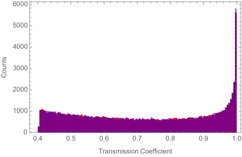
Figure 3: (Color online) Histogram of $\sin^{2}\theta_{N}.$ Each scatterer has the potential $V$ chosen at random, uniformly over the interval $[-0.3,0.3].$ The angle $\theta$ associated with a scatterer is $\cos^{-1}(|V|/\sqrt{V^{2}+4\sin^{2}k}),$ where we have chosen the energy $2\cos k$ to be 1.2. The phase $\phi$ between each scatterer and its predecessor is chosen to be a uniform random variable over the interval $0<\phi<\theta.$ The histogram is plotted for $10^{5}$ random lattices with $N=100$ scatterers (blue) and $N=10,000$ scatterers (red). No significant difference is seen between the two.

Figure 3 shows numerical results for the transmission coefficient $\sin^{2}\theta_{N}.$ Histograms for $N=100$ and $N=10000$ show no significant difference, indicating that the $N\rightarrow\infty$ limit has been reached. Each scatterer has a $S$-matrix of the form of Eq.(5) with $V$ chosen uniformly over the interval $=0.3<V<0.3$ and $2\sin k=1.6.$ As discussed at the end of Section II.1, the angle $\theta$ for each scatterer is chosen to be in the first or fourth quadrant, and in Eq.(13), it can be chosen to be in the first quadrant without loss of generality. Since the allowed range of $V$ is small, all the scatterers are weak, and $\theta$ lies within a small interval near $\pi/2.$ The angle $\phi$ is chosen randomly, as described earlier. Under these conditions, one can show analytically that the distribution for $\sin^{2}\theta_{N}$ has a lower cutoff which is greater than zero, as seen in the figure.

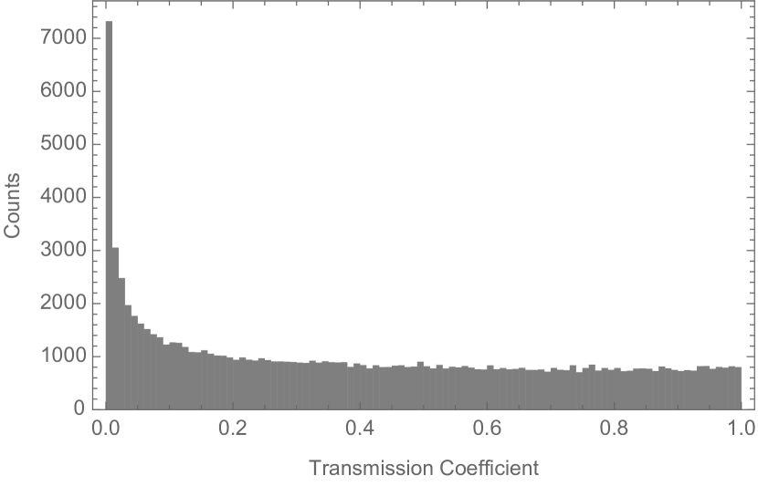
Figure 4: Histogram of $\sin^{2}\theta_{N}.$ The angle $\theta$ for each scatterer is chosen to be a uniform random variable in the first quadrant, and the angle $\phi$ is a uniform random variable between 0 and $\theta.$ The histogram is constructed from $10^{5}$ lattices with $N=1000$; increasing $N$ does not change this significantly. Although there is a peak in the histogram at $\sin^{2}\theta_{N}=0,$ possibly a divergence, there is a long tail to the distribution, and $\langle\sin^{2}\theta_{\infty}\rangle$ is non-zero.

On the other hand, if we consider $\theta$ to be a uniform random variable in the interval $(0,\pi/2]$ (with $0<\phi<\theta,$), $\langle\cot^{2}\theta\rangle$ diverges and the proof that $\langle\cot^{2}\theta_{N\rightarrow\infty}\rangle$ is finite is not valid. Nevertheless, as seen in Figure 4, $\langle\sin^{2}\theta_{N\rightarrow\infty}\rangle$ is finite; the peak at the origin of the distribution is accompanied by a broad flat tail.

From the arguments above, one might think that a random lattice that is designed to have a $O(1)$ transmission coefficient at a certain energy should have an $O(1)$ transmission coefficient (i.e. delocalized states) over a band of energy, since the $S$-matrix for each scatterer as well as the phase introduced by a path length $L$ evolve continuously as a function of the wavevector $k.$ However, this is not the case. The path-dependent phase $\phi$ associated with the interval between the $N^{{\rm th}}$ and $(N+1)^{{\rm th}}$ scatterers was defined to be $\phi=2k(L+1)+\gamma+\gamma_{N}-\delta_{N}.$ Once the length $L$ of the interval has been optimized for some $k,$ to ensure that $0<\phi<\theta,$ a small change in $k$ could change $\gamma_{N}-\delta_{N}$ by a large amount if $N$ is large, so that the condition $0<\phi<\theta$ would no longer be satisfied. Numerical simulations reveal this to be the case: although the prescription above allows one to obtain $O(1)$ transmission at any chosen energy, the transmission coefficient drops off as one moveas away from this energy, and decays as a function of $N$ for any energy other than the energy for which the structure is designed.

IV Conclusion

We have shown that a one dimensional conductor with correlated disorder has an extended state that is unrelated to any symmetry of the problem and exists despite the fact that the individual scatterers are not effectively transparent as in previous examples of one dimensional delocalization. Conceptually the delocalized structure is constructed scatterer by scatterer so it is natural to expect that it can be most readily realized experimentally as a stacking of films much like a one dimensional photonic crystal photonic . A possible application of such a structure is as an extremely narrow band filter for light. In contrast to a photonic crystal the structure does not have to be engineered with precision; the randomness is in fact essential to the operation of the filter. Cold atoms are another experimental arena for localization studies wherein correlated disorder may be realizable cold . An interesting analog of Anderson localization is provided by the phenomenon of dynamical localization in kicked quantum rotors prange . Whether the ideas discussed in this paper can be exported to that context or generalized to two and higher dimensions are interesting open questions.

References

- (1) P.W. Anderson, “Absence of Diffusion in Certain Random Lattices”, Phys. Rev. 109, 1492 (1958).
- (2) E. Abrahams, P.W. Anderson, D. Licciardello, and T.V. Ramakrishnan, “Scaling Theory of Localization: Absence of Quantum Diffusion in Two Dimensions”, Phys. Rev. Lett. 42, 673 (1979).
- (3) P.A. Lee and T.V. Ramakrishnan, “Disordered Electronic Systems”, Rev. Mod. Phys. 57, 287 (1985).
- (4) For an entry point into the vast literature see for example, A. Lagendijk, B. van Tiggelen and D. Wiersma, “Fifty years of Anderson Localization”, Physics Today 62, 24 (2009); E. Abrahams (ed), 50 Years of Anderson Localization (World Scientific, Singapore, 2010).
- (5) K. Ishii, “Localization of Eigenstates and Transport Phenomena in 1D Disordered Systems”, Progr. Theor. Phys. Suppl. 53, 77 (1971).
- (6) P.W. Anderson, D.J. Thouless, E. Abrahams, D.S. Fisher, “New method for a scaling theory of localization”, Phys. Rev. B22, 3519 (1980).
- (7) C.W.J. Beenakker, “Random Matrix theory of quantum transport”, Rev. Mod. Phys. 69, 731 (1997).
- (8) A.J. McKane and M. Stone, “Localization as an alternative to Goldstone’s theorem”, Annals of Physics 131, 36 (1981).
- (9) K.B. Efetov, Supersymmetry in Disorder and Chaos (Cambridge Univ Press, 1996).
- (10) L. Balents and M.P.A. Fisher, “Delocalization transition via supersymmetry in one dimension”, Phys. Rev. B56, 12970 (1997); H. Mathur, “Feynman’s propagator applied to network models of localization”, Phys. Rev. B56, 15794 (1997).
- (11) A. Altland and M.R. Zirnbauer, “Nonstandard symmetry classes in mesoscopic normal superconducting hybrid structures”, Phys. Rev. B55, 1142 (1997).
- (12) P.W. Brouwer, A. Furusaki, I.A. Gruzberg and C. Mudry, “Localization and Delocalization in Dirty Superconducting Wires”, Phys. Rev. Lett. 85, 1064 (2000).
- (13) D. Dunlap, H.-L. Wu, and P. Phillips, “Absence of Localization in a Random Dimer Model”, Phys. Rev. Lett. 65, 88 (1990).
- (14) H.U. Baranger and A.D. Stone, “Electrical linear-response theory in an arbitrary magnetic field: A new Fermi-surface formulation”, Phys. Rev. B40, 8169 (1989).
- (15) P.D. Kirkman and J.B. Pendry, “The Statistics of One-Dimensional Resistances”, J Phys C17, 4327 (1984).
- (16) J.D. Joannopoulos, S.G. Johnson, J.N. Winn and R.D. Meade, Photonic Crystals: Molding the Flow of Light (Princeton University Press, 2nd ed, 2008).
- (17) S. Kondov et al., “Three dimensional Anderson localization of ultracold matter”, Science 334, 66 (2011); F. Jendrzejewski et al., “Three dimensional localization of ultracold atoms in an optical disordered potential”, Nat. Phys. 8, 398 (2012); G. Semeghini et al., “Measurement of the mobility edge for 3D Anderson localization”, Nat. Phys. 11, 554 (2015).
- (18) S. Fishman, D.R. Grempel and R.E. Prange, “Quantum dynamics of a nonintegrable system”, Phys. Rev. A29, 1639 (1984); F.L. Moore, J.C. Robinson, C. Bharucha, P.E. Williams and M.G. Raizen, “Observation of Dynamical Localization in Atomic Momentum Transfer: A New Testing Ground for Quantum Chaos”, Phys. Rev. Lett. 73, 2974 (1994).