Learning an arbitrary mixture of two multinomial logits
Abstract.
In this paper, we consider mixtures of multinomial logistic models (MNL), which are known to -approximate any random utility model. Despite its long history and broad use, rigorous results are only available for learning a uniform mixture of two MNLs. Continuing this line of research, we study the problem of learning an arbitrary mixture of two MNLs. We show that the identifiability of the mixture models may only fail on an algebraic variety of a negligible measure. This is done by reducing the problem of learning a mixture of two MNLs to the problem of solving a system of univariate quartic equations. We also devise an algorithm to learn any mixture of two MNLs using a polynomial number of samples and a linear number of queries, provided that a mixture of two MNLs over some finite universe is identifiable. Several numerical experiments and conjectures are also presented.
Key words : complexity, cubic equations, identifiability, mixture models, multinomial logits, multivariate polynomials, polynomial identifiability, quartic equations, symbolic computations.
1. Introduction
This paper is concerned with the problem of learning a mixture of two multinomial logistic models from data. Understanding an individual, or a user’s rational behavior when facing a list of alternatives is a classical topic in economic theory. In the era of data deluge, it has wide applications, especially for recommender systems where a user decides which of several competing products to purchase, and companies like Amazon, Netflix and Yelp look for which products are most relevant to a specific user. A powerful tool to study user behavior is discrete choice models, and we refer to McFadden [20, 21, 22, 23] for the modern literature. The most well-studied class of discrete choice models are the class of random utility models, which find roots in the work of Thurstone [31], and were formally introduced by Marschak [19]. The book of Train [32] contains a thorough review on this subject. Mixtures of multinomial logistic models (also known as mixed logits) are a family of parametric random utility models, which have been widely used since 1980 [4, 7], following earlier works of Bradley-Terry [5], and Luce-Plackett [18, 28] on the multinomial logits. Despite its broad use in practice, e.g. the EM algorithm [10], there are few works on efficient algorithms to learn any non-trivial mixture of multinomial logistic models. Chierichetti et al. [9] took the first step to develop polynomial-time algorithms to learn a uniform mixture of two multinomial logits. They also pointed out that generalizing the results to non-uniform mixtures, or mixtures of more than two components is challenging.
The purpose of this paper is to go beyond the uniform mixture, and study the problem of reconstruction and polynomial-time algorithms to learn an arbitrary mixture of two multinomial logits from user data. To proceed further, we give a little more background. A multinomial logistic model, or simply an MNL over a universe is specified by a mapping from any non-empty subset to a distribution over . The set is referred to as the choice set or the slate, from which a user selects exactly one item. The MNL requires a weight function which gives a positive weight to each item in the universe . The model then assigns probability to each proportional to its weight:
One can regard as the conditional probability of selecting item given the alternatives in . We normalize the weight function by , so where is the -simplex with the number of items in . Given sufficient data of slates with resulting choices of , it is possible to estimate the weight via maximum likelihood estimation. The underlying problem is convex, and is easy to solve by gradient methods.
In spite of simple interpretation and computational advantages, MNL is criticized for being too restrictive on the model behavior across related subsets, and thus lack of flexibility. This drawback is due to the fact that MNL is defined as a family of functions mapping any to a distribution over , based on a single fixed weight function. One way to resolve this issue is to remove the constraint that the likelihood of each item is always proportional to a fixed weight. The aforementioned random utility model does the job: it is defined by a distribution over vectors, where each vector assigns a value to each item of . A user then draws a random vector from this distribution, and selects the item of with the largest value. McFadden and Train [24] observed that any random utility model can be approximated arbitrarily close by a mixture of MNLs. Thus, learning general random utility models reduces to learning mixtures of MNLs. This is the reason why mixtures of MNLs are widely recognized by practitioners. However, almost all existing learning approaches are empirical, and there are few provable results on learning non-trivial mixtures of MNLs. The only exception is [9], where the authors resolved positively the problem of leaning a uniform mixture of MNLs, assuming an oracle access to the true distributions over all choice sets. Indeed, they do not learn the mixture of MNLs from sample data. Here we take a further step to study a possibly non-uniform mixture of two MNLs given access to samples. We provide a few positive results on optimal learning algorithms.
The object of interest is specified by the triple , where are two weight functions, and is the mixing weight. A -mixture of two MNLs assigns to item in the set the probability
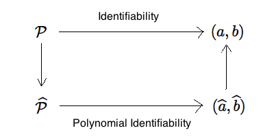
The goal of the learning problem is to reconstruct the parameters from the sample outcomes of the slate induced by the mixture. In this paper, we assume that the mixing weight is known. So the problem consists of learning the weight functions in a -mixture of MNLs. Our program is illustrated by the following diagram, which consists of two basic problems:
-
(i)
Identifiability: Is the -mixture model uniquely characterized by a pair of weights ? That is, if the -mixtures of MNLs and agree on each then , .
-
(ii)
Polynomial identifiability: Given that the -mixture model is identifiable, is there an algorithm to learn or to estimate the weights with polynomial running time and using a polynomial number of samples?
We start with the identifiability of the -mixture of two MNLs. The main result of [9] showed that for , if , any uniform mixture of two MNLs is identifiable; there is an algorithm which learns any uniform mixture of two MNLs with queries to the oracle returning the -mixture distribution over items of the slate. Theorem 2.1 below contains more detailed statements. The idea relies on the fact that any uniform mixture of two MNLs over a -item universe is identifiable, and one can reconstruct the weight functions by querying to - and -slates, i.e. subsets with . But this algorithm fails for a non-uniform mixture of two MNLs, since a non-uniform mixture of two MNLs on a -item universe is not necessarily identifiable (see Section 3, or [9, Theorem 3]). Nevertheless, the latter is ‘rarely’ the case which is the first main result of this paper.
Theorem 1.1.
Let , and . If the -mixtures of MNLs and agree, i.e. have the same distribution on each , then
where is some polynomial specified later in the proof.
Theorem 1.1 shows that the identifiability of a mixture of two MNLs may only fail on some algebraic variety . We refer to the books of Sturmfels [25, 30] for a gentle introduction to algebraic geometry with focus on the computational aspects. More important than the theorem itself is the way to construct the multivariate polynomials . As we will see later, this and the problem of learning a mixture of two MNLs essentially boils down to the problem of finding the common roots of some univariate quartic equations. Unlike [9], we adopt purely an equation-solving approach which is more natural and transparent.
Now we turn to the polynomial identifiability of the mixture model. There is a rich body of literature, e.g. [1, 2, 11, 16, 26] on the polynomial identifiability of Gaussian mixture models. The algorithms use the method of moments, which relies on rich structure in lower-order moments of the Gaussian mixture model. However, this low rank property is not enjoyed by the mixture of (two) MNLs, and lower moments are not sufficient to characterize or to approximate the model parameters. In fact, it is even unknown whether all -mixtures of two MNLs over a -item universe are identifiable. Based on numerical experiments, we conjecture the latter to be true. This motivates the following -identifiability assumption for some , which will be used to devise a polynomial learning algorithm for the -mixture model.
Assumption 1.2 (-identifiability).
The -mixtures of two MNLs over a -item universe are identifiable.
Theorem 1.3.
Let Assumption 1.2 hold. For , consider a -mixture of two MNLs over an -item universe with the weight functions . Also assume that there are such that for ,
| (1.1) |
Let be sufficiently small. There is an adaptive algorithm which outputs weights such that
with high probability, by using
-
•
(sample complexity) independent samples of - and -slates.
-
•
(query complexity) queries to the estimated - and -slates.
Theorem 1.3 shows the polynomial identifiability of the -mixture model under suitable conditions. In addition to Assumption 1.2, we postulate that the items in the slate are comparable to each other, which leads to (1.1). Note that our algorithm takes half the number of queries that the adaptive algorithm in [9] uses to learn a uniform mixture of two MNLs, but it requires querying to large slates.
The contributions of the paper are threefold:
-
(i)
We show that the identifiability of the mixture model does not cause much a problem, and it may only fail on some ‘small’ algebraic variety of a negligible measure. This is important to develop further Baysian nonparametric models, where user choice is modeled by a mixture of random MNLs. That is, both and are random, and are drawn from some distributions.
-
(ii)
We show that identifying or learning a mixture of two MNLs is reduced to solving a system of univariate quartic equations. This gives a possible way to prove Assumption 1.2 – the identifiability of any mixture of two MNLs over some finite universe.
-
(iii)
We provide a learning algorithm for an arbitrary mixture of two MNLs, which requires a polynomial number of samples, and a linear number of queries. To the best of our knowledge, this paper is the first one that discusses the polynomial identifiability of mixtures of MNLs.
As will be clear in the later proof, even the mixing parameter is unknown, Theorem 1.1 holds in the sense that the identifiability of may only fail on a negligible set. However, it is not clear how to estimate efficiently the parameter from sample data. The remaining issues, which seem to be technically challenging, are polynomial conditions in nature. We hope that this work will draw attention to experts of algebraic geometry and symbolic computations, so that advanced techniques in these domains can be used or developed to solve the conjectures in the paper.
To conclude the introduction, let us mention a few relevant references. There are a line of works discussing heuristic approaches to learn mixtures of MNLs by simulation [12, 14, 17, 32]. Mixtures of MNLs have also been studied in the context of revenue maximization by [3, 29]. More related to this work are [8, 27, 33, 34], where different oracles are assumed. We refer to [9, Section 2] for a more detailed explanation of the aforementioned references, and various pointers to other related works.
The rest of the paper is organized as follows. Section 2 collects results related to mixtures of MNLs, and compares with our results. Section 3 warms up with a discussion of the mixture of two MNLs over a -item universe. Section 4 studies the general problem of learning a mixture of two MNLs over an -item universe. Section 5 gives the conclusion.
2. Preliminaries, existing results and comparison
This section provides background on the multinomial logit models, and recalls a few existing results in comparison with Theorems 1.1 and 1.3. We follow closely the presentation in Chierichetti et al. [9]. Consider the -item universe, whose items are labeled by . A slate is a non-empty subset of , and a -slate is a slate of size .
A multinomial logit, or simply -MNL is determined by a weight function , where is the -simplex, with the set of nonnegative real numbers. In this choice model, given a slate , the probability that item is selected is given by
| (2.1) |
One can also take a weight function , and normalizing each by will not affect the selection probability (2.1). A mixture of two multinomial logits, or simply -MNL is specified by two weight functions , and a mixing parameter in such a way that the probability that item is selected in the slate is
| (2.2) |
For later simplification, we use the parameter instead of as the mixing weight. So given a slate , first chooses the weight function with probability and with probability , and then behaves as the corresponding -MNL. For ease of presentation, we drop the superscript and write instead of if there is no ambiguity. If or , the choice model is called a uniform -MNL.
In [9], the authors considered the problem of reconstructing the parameters of the uniform -MNL, assuming an oracle access to for all and . Their results are summarized in the following theorem.
Theorem 2.1.
Let , and , be two uniform -MNL over . Then:
-
(i)
and agree on each , i.e. for each if and only if , , or , .
-
(ii)
Any adaptive algorithm for -MNL which queries to -slates requires queries.
-
(iii)
There is an adaptive algorithm to learn a uniform -MNL with queries to - and -slates.
As explained in the introduction, a weakness of [9] is that they assume the distribution of the slate is known. So they learn from the oracle distribution, not from the user samples. In order to adapt the results of [9] for samples, we need the following elementary result.
Lemma 2.2.
Let be a distribution over , and be the empirical distribution from independent samples of :
where are i.i.d. copies from the distribution . Assume that there are such that
| (2.3) |
If , then with probability ,
Proof.
As an easy consequence of Lemma 2.2 and [9, Theorems 5], the following result shows the polynomial identifiability of the uniform mixture of two MNLs.
Theorem 2.3.
Consider a uniform mixture of two MNLs over an -item universe with the weight functions . Assume that (1.1) holds for . Let be sufficiently small. There is an adaptive algorithm which outputs weights such that
with high probability, by using
-
•
(sample complexity) independent samples of - and -slates.
-
•
(query complexity) queries to the estimated - and -slates.
Now we compare Theorem 2.3 with Theorem 1.3. For a uniform mixture of two MNLs, it requires samples of - and -slates to achieve a given accuracy . This has advantage in both sample size and slate size over the samples of -slates in our algorithm. However, the algorithm in [9] for the uniform mixture relies on the identifiability of the model over a -item universe, which is not available for an arbitrary mixture of two MNLs. Given the estimated slates, our algorithm for an arbitrary mixture requires half the number of queries that is used to learn a uniform mixture model. It is interesting to know whether there is an algorithm which only queries to small slates with polynomial sample complexity, and linear query complexity. We leave the problem open.
3. Identifiability of -MNL on the -item universe
In this section, we study a -MNL on the -item universe .
Assume that the mixing parameter is known.
So we only need to reconstruct the -MNL weights and .
As pointed out in [9], for the oracle
does not uniquely determine the weights .
The main point of Theorem 1.1 is that this situation rarely happens, and we can characterize the instances
where the uniqueness fails.
As will be seen in Section 4, the computation yielding the non-uniqueness characterization for is
a building block to study the identifiability of -MNL for .
Let the oracle be generated from the weights , e.g. . To simplify the notations, we denote . The problem involves solving the following system of equations:
| (3.1a) | |||
| (3.1b) | |||
| (3.1c) | |||
So there are unknowns and 11 equations, from (3.1a), from (3.1b) and from (3.1c). Since and , there are linearly independent equations. Implicitly, there are more inequalities: , for . The following lemma provides a simple way to narrow down the possible solutions to (3.1).
Lemma 3.1.
Proof.
By (3.1b)–(3.1c), it is easy to see that determines the remaining variables by
| (3.2) | ||||
Note that (3.1a) can be rewritten as
| (3.1a’) |
Specializing (3.1a’) to , and using (3.2) to express in terms of , we get
| (3.3) |
where is a quadratic function of , and is linear in . Further specializing (3.1a’) to , and using (3.2)–(3.3) to express in terms of , we have
| (3.4) |
The first term on the l.h.s. of (3.4) is a quartic polynomial in , and the other two terms are cubic polynomials in . ∎
The main point of Lemma 3.1 is to reduce the system of equations (3.1) to that only involving the -tuple :
| (3.5a) | |||
| (3.5b) | |||
Moreover, solving the system of equations (3.5) is equivalent to solving a univariate quartic equation. We call the equations (3.5a)–(3.5b) the -system. Note that if and , then similar to (3.3) we can express in terms of , and hence all the other variables in terms of by (3.2). If and , it is clear that all the other variables are uniquely determined by (3.2).
Recall that the values of are generated from some weights . This implies that the quartic equation given by (3.4) has at least one real root in , which is . Here the subscript ‘’ indicates that the polynomial is associated with the -system. Let
which is a cubic polynomial whose coefficients are rational functions of . Therefore, the identifiability of a -MNL on the -item universe, or equivalently the uniqueness of the solution to the system of equations (3.1) reduces to the problem if the cubic polynomial has a real roots and ; if the corresponding -tuple given by (3.2)–(3.3) solves (3.1). Algorithmically, this is rather easy to verify: Cardano’s formula [6] solves any cubic equation. Then it suffices to check if the corresponding , and if the equation , which is part of (3.1) but not in (3.5) holds.
Now we show that it is rarely the case that the system of equations (3.1) has more than one solution . In fact, it is even true that (3.1) can barely have more than one solution .
Proof of Theorem 1.1 (n = 3).
Consider associated with the -system, and associated with the -system. Observe that the system (3.1) has only one solution if the polynomials and have only one common root , or equivalently the polynomials and do not have any common root. It is well known [15, Lemma 3.6] that the latter holds if and only if
where is the resultant of and , the determinant of a Sylvester matrix whose entries are the coefficients of and . Recall that the coefficients of , are rational functions of . By letting be the polynomial corresponding to the numerator of , we have
That is, the uniqueness of the solution to (3.1) may fail only for those on the algebraic variety . ∎
Of course, it is rather impossible to put down the expression of by hand. With the help of Mathematica, we get an expression of as follows:
![[Uncaptioned image]](/html/2007.00204/assets/n3.png)
But it seems that even Mathematica finds it challenging to expand, or to simplify the above large expression.
To conclude this section, we go back to the cubic polynomial . This polynomial has either real roots, or real root and complex conjugate roots. Since we are only concerned with the real roots of , it is natural to ask whether can have real roots for some and . The point is that if has only real root, the analysis may further be simplified. It turns out that this question is subtle. It is known [6] that has real roots if the discriminant of is nonnegative. Note that the discriminant of is a function of . For , the functions FindInstance and NSolve in Mathematica do not find any -tuple such that the discriminant of is nonnegative. Moreover, the function NMaximize finds numerically the maximum of the discriminant of over , which is . These observations suggest that have only real root when . However, for and , Mathematica finds that has real roots: . Based on many experiments, we conjecture that there is a threshold such that for , has only real roots whatever the values of , and for , can have either or real roots depending on the values of .
4. Learning -MNL on the -item universe
This section is devoted to the study of a -MNL over for . The key idea is to reduce the system of equations over unknowns to -systems. This also gives a promising way to prove the identifiability of a -MNL on for some possible . The following result records the general structure of learning a -MNL over items. Recall the definitions of and for from Section 3.
Proposition 4.1.
Let , and be a -MNL over . Assume that is known. Then learning is equivalent to solving the following system of equations with unknowns :
| (4.1a) | |||
| (4.1b) | |||
So there are equations, and at most of these equations are linearly independent.
Proof.
Note that for each with , (4.1a) contributes equations, and of these equations are linearly independent. The result follows from the well known identities and . ∎
The following -system is an obvious extension of (3.5) to the -item universe:
| (4.2a) | |||
| (4.2b) | |||
Similar to Lemma 3.1, solving the system of equations (4.1) boils down to solving a univariate quartic equation by using -systems.
Lemma 4.2.
Assume that solves (4.1), and . Then:
-
(i)
If for each there exists a set containing such that , then .
-
(ii)
Otherwise, assume without loss of generality for any set containing . Then each of can be written as a simple function of , and solves a quartic equation.
Proof.
Part is straightforward. For part , consider the -system for all . By Lemma 3.1, are fully determined by , and solves the quartic equation associated with the -system. ∎
Basically, Lemma 4.2 shows that the system (4.1) with approximately equations has at most solutions. This simplification only makes use of equations, which involves those in (4.1a) with . That is, queries to -slates and -slates. Theorem 1.1 is then a consequence of Lemma 4.2.
Proof of Therorem 1.1 (general ).
We follow the notations in Section 3 which proves the result for . Similarly, define the polynomials , associated with the -system. Recall that the coefficients of , are rational functions of . By Lemma 4.2, if the system of equations (4.1) has more than one solution, then the polynomials have a common root. The latter implies that each pair have a common root, which is equivalent to
where is the resultant of two polynomials. Let be the multivariate polynomial in corresponding to the numerator of . We have
In particular, one can take so that (4.1) has the unique solution when . ∎
There are many ways to build in Theorem 1.1. One can take for any subset of , e.g. in the previous proof, or just for some . Given , it is relatively easy to check numerically if . But as mentioned in Section 3, even in the simple case (with variables), Mathematica cannot output the expression of , let alone doing further symbolic computations.
Now we give a simpler when . Consider the equations in (4.1a) relating only . For , in addition to the -system there is one more:
| (4.3) |
By injecting (3.2)–(3.3) into (4.3), we get with another quartic polynomial. Let be the corresponding cubic polynomial. Another simple choice for is the numerator of , which Mathematica outputs:
![[Uncaptioned image]](/html/2007.00204/assets/n4.png)
Such defined is a polynomial in variables, and is apparently simpler than the previous choices for . The expression of this has more than terms, and the maximum degrees of appearing in are respectively. An interesting question is whether is empty for all . If so, the system of equations (4.2)–(4.3) has a unique solution which implies that any -MNL over is identifiable for . Unfortunately, the following example shows it is not the case. For , and , , the system of equations (4.2)–(4.3) gives two solutions: , , and , .
In principle, determining if a -MNL over is identifiable, or if the system of equations (4.1) has only one solution reduces to determining if a set of about univariate cubic equations have a common root. The latter is equivalent to whether the resolvent of these cubic polynomials is zero, and this amounts to a fairly large number of multivariate polynomial equations on , see e.g. [13, Section 7]. So as increases, the set of for which the system of equations (4.1) has more than solution becomes more and more restrictive. It is believable that there is a threshold such that (4.1) has only one solution for . Based on many experiments, we conjecture that ; that is, any -MNL over for is identifiable. We leave this puzzle to interested readers.
To finish this section, we prove Theorem 1.3 on the polynomial identifiability of the mixture model.
Proof of Theorem 1.3.
We start with the identifiability, i.e. learn the weights from the oracle . Note that solves (4.1a) for but with possibly , . By the -identifiability, takes the form: , for , where is the unique solution to (4.1) for , and and have yet to be determined. It requires queries to find . For instance, by Lemma 4.2, there are at most possible solutions associated with the -system, and a quartic equation is easily solved by Ferrari’s method [6]. Then it suffices to check which one of these solutions satisfy other equations. Next for each , consider the -system (4.2) which has queries. By Lemma 4.2, can be expressed in terms of . So the condition determines . Similarly, by expressing in terms of , the condition specifies . In total, it requires queries to learn the mixture model.
Now we consider learning the weights from samples . By Lemma 2.2, if , we have for . Further by assumption (1.1), we get
| (4.4) |
for some . The idea is to control the ratio uniformly in . It is easily seen that for , the term on the left side of (4.4) is controlled by , and we write . Since is not the oracle, the equation (4.1) with and (instead of ) does not necessarily have a unique admissible solution. By continuity of complex roots with respect to polynomial coefficients, for sufficiently small, there is a unique root with real part between and the smallest imaginary part – this gives and then . We repeat the procedure in the previous paragraph by substituting with . By the implicit function theorem, we have , , and . As a result,
Similar results hold for the weight function . ∎
5. Conclusion
In this paper, we study the problem of learning an arbitrary mixture of two multinomial logits. We have proved that the identifiability of the mixture models is less problematic, since it may only fail on a set of parameters of a negligible meausure. The proof is based on a reduction of the learning problem to a system of univariate quartic equations. We also proposed an algorithm to learn any mixture of two MNLs using a polynomial number of samples and a linear number of queries, under the assumption that a mixture of two MNLs over some finite universe is identifiable.
The paper also leaves a few problem for future research. For instance,
- (i)
-
(ii)
devise an algorithm to learn an arbitrary mixture of two MNLs using only small slates with polynomial samples and queries.
-
(iii)
consider the identifiability issue for both the mixing parameter and the weight functions .
-
(iv)
study the problem of learning a mixture of more than two multinomial logits.
We hope that our work will trigger further developments on the mixture models.
References
- [1] A. Anandkumar, R. Ge, D. Hsu, S. M. Kakade, and M. Telgarsky. Tensor decompositions for learning latent variable models. J. Mach. Learn. Res., 15:2773–2832, 2014.
- [2] A. Bhaskara, M. Charikar, and A. Vijayaraghavan. Uniqueness of tensor decompositions with applications to polynomial identifiability. In Conference on Learning Theory, pages 742–778, 2014.
- [3] J. Blanchet, G. Gallego, and V. Goyal. A Markov chain approximation to choice modeling. Oper. Res., 64(4):886–905, 2016.
- [4] J. H. Boyd and R. E. Mellman. The effect of fuel economy standards on the US automotive market: an hedonic demand analysis. Transportation Research Part A: General, 14(5-6):367–378, 1980.
- [5] R. Bradley and M. Terry. Rank analysis of incomplete block designs: I. The method of paired comparisons. Biometrika, 39(3/4):324–345, 1952.
- [6] G. Cardano. Ars Magna or The Rules of Algebra. Dover Publications, Inc., New York, 1993. Translated from the Latin and edited by T. Richard Witmer.
- [7] N. S. Cardell and F. C. Dunbar. Measuring the societal impacts of automobile downsizing. Transportation Research Part A: General, 14(5-6):423–434, 1980.
- [8] F. Chierichetti, R. Kumar, and A. Tomkins. Discrete choice, permutations, and reconstruction. In Symposium on Discrete Algorithms, pages 576–586, 2018.
- [9] F. Chierichetti, R. Kumar, and A. Tomkins. Learning a mixture of two multinomial logits. In International Conference on Machine Learning, pages 961–969, 2018.
- [10] A. P. Dempster, N. M. Laird, and D. B. Rubin. Maximum likelihood from incomplete data via the EM algorithm. J. Roy. Statist. Soc. Ser. B, 39(1):1–38, 1977.
- [11] R. Ge, Q. Huang, and S. M. Kakade. Learning mixtures of Gaussians in high dimensions. In Proceedings of the 2015 ACM Symposium on Theory of Computing, pages 761–770, 2015.
- [12] Y. Ge. Bayesian Inference with Mixtures of Logistic Regression: Functional Approximation, Statistical Consistency and Algorithmic Convergence. PhD thesis, Northwestern University, Evanston, USA, 2008.
- [13] R. Goldman. Algebraic geometry and geometric modeling: insight and computation. In Algebraic Geometry and Geometric Modeling, Math. Vis., pages 1–22. Springer, Berlin, 2006.
- [14] C. A. Guevara and M. E. Ben-Akiva. Sampling of alternatives in logit mixture models. Transportation Research Part B: Methodological, 58:185–198, 2013.
- [15] J. Harris. Algebraic Geometry: A First Course, volume 133 of Graduate Texts in Mathematics. Springer-Verlag, New York, 1995.
- [16] D. Hsu and S. M. Kakade. Learning mixtures of spherical Gaussians: moment methods and spectral decompositions. In Proceedings of the 2013 ACM Conference on Innovations in Theoretical Computer Science, pages 11–19, 2013.
- [17] M. Hurn, A. Justel, and C. P. Robert. Estimating mixtures of regressions. J. Comput. Graph. Statist., 12(1):55–79, 2003.
- [18] R. D. Luce. Individual Choice Behavior a Theoretical Analysis. John Wiley & Sons Inc., 1959.
- [19] J. Marschak. Binary choice constraints on random utility indicators. In Stanford Symposium on Mathematical Methods in the Social Sciences, pages 312–329.
- [20] D. McFadden. Conditional Logit Analysis of Qualitative Choice Behavior, pages 105–142. Academic Press, New York, 1974.
- [21] D. McFadden. Econometric Models of Probabilistic Choice, pages 198–272. MIT Press, Cambridge, 1981.
- [22] D. McFadden. Qualitative response models, pages 1–38. Econometric Society Monographs. Cambridge University Press, 1983.
- [23] D. McFadden. Economic Choices. American Economic Review, 91(3):351–378, 2001.
- [24] D. McFadden and K. Train. Mixed MNL models for discrete response. Journal of Applied Econometrics, 15(5):447–470, 2000.
- [25] M. Michałek and B. Sturmfels. Invitation to Nonlinear Algebra. 2020+. Available at https://personal-homepages.mis.mpg.de/michalek/NonLinearAlgebra.pdf.
- [26] A. Moitra and G. Valiant. Settling the polynomial learnability of mixtures of Gaussians. In 51st Annual Symposium on Foundations of Computer Science, pages 93–102. 2010.
- [27] S. Oh and D. Shah. Learning mixed multinomial logit model from ordinal data. In Advances in Neural Information Processing Systems, pages 595–603, 2014.
- [28] R. Plackett. The analysis of permutations. Applied Statistics, pages 193–202, 1975.
- [29] P. Rusmevichientong, D. Shmoys, C. Tong, and H. Topaloglu. Assortment optimization under the multinomial logit model with random choice parameters. Production and Operations Management, 23(11):2023–2039, 2014.
- [30] B. Sturmfels. Solving systems of polynomial equations, volume 97 of CBMS Regional Conference Series in Mathematics. Conference Board of the Mathematical Sciences, Washington, DC, 2002.
- [31] L. Thurstone. A law of comparative judgment. Psychological Review, 34(4):273, 1927.
- [32] K. E. Train. Discrete choice methods with simulation. Cambridge University Press, Cambridge, second edition, 2009.
- [33] Z. Zhao, P. Piech, and L. Xia. Learning mixtures of Plackett-Luce models. In International Conference on Machine Learning, pages 2906–2914, 2016.
- [34] Z. Zhao and L. Xia. Learning mixtures of Plackett-Luce models from structured partial orders. In Advances in Neural Information Processing Systems, pages 10143–10153, 2019.