Instability induced by exchange forces in a 2-D electron gas in a magnetic field with uniform gradient

Abstract

The exchange interaction is investigated theoretically for electrons confined to a 2-D sample placed in a linearly varying magnetic field perpendicular to the plane. Unusual and interesting behavior is predicted: starting from zero electrons, as one adds electrons to the system the maximum distance an electron can travel transverse to the $B_{z}=0$ line (i.e. the system’s width) increases continuously but this width will subsequently begin shrinking at some critical number.However this collapse will be reversed as the number crosses another critical value, which we estimate here. For electron parameters typical for 2DEG’s, the instability could be observable at sufficiently low electron densities. A Hartree Fock equation is derived. We also show that in an appropriate asymptotic limit this leads to an approximately local potential. One key lesson is that the exchange interaction is large and cannot be reasonably excluded from any valid theoretical investigation.

.1 Introduction

Cooperative effects in many body systems have been investigated since the early days of quantum mechanics with mean field theory being a critical and often highly successful tool in the investigation of atomic, molecular, and nuclear structure Negele . The “Fermi hole” coming from repulsion of identical fermions with the same spin enables one to tackle a system that would otherwise be intractable. A direct consequence is the exchange force which is critically important in determining many body properties. While many systems have been investigated in mean field theory, the particular system to be discussed below has not. The present work is a first attempt to uncover the behavior of this particular many body system teetering at the edge of instability. As such it adds to the stock of existing systems that are at least partially solvable Negele ,Vignale .

Considered here is a two dimensional electron gas (2-DEG) such as created by using a GaAs/GaAlAs heterostructure. It is subjected to a perpendicular magnetic field whose strength varies linearly from one edge to the other. Müller Muller carried out the first calculation of free electrons with levels filled up to $\sim 14$ meV   and excitation levels $n\gtrsim$ $30$. The sample boundary promotes electrons to the next level. In contrast there will be no sample edge in what we consider here. As such it is a far simpler, cleaner system. Using qualitative reasoning Müller also pointed out that the classical electron trajectory is snake-like and weaves around the $B_{z}=0$ line. Other authors (including the present author) Reijners1 Reijners2 Nogaret Hoodbhoy Puja followed up with various other calculations but none included the exchange force. As it turns out, the omission is crucial; exchange effects are so large that calculations not including them might need to be reassessed or redone. Why they were omitted is obvious: calculating the exchange energy for electrons in a uniform magnetic field is tedious but can still be found in textbooks such as refVignale where they turn out to be substantial. A similar calculation for the non-uniform case under consideration here seems dauntingly complicated and seems not to have been addressed in the literature. Any insight into the role of exchange for this particular system would therefore be of interest.

Consider the following gedanken experiment on a rectangular surface in the $x-y$ plane along which electrons can move with a long mean path between collisions. The sample is placed in a $z$-directed $B$ field, $\vec{B}=B^{\prime}y$ $\hat{e}_{z}.$ Starting from zero, electrons are added one by one by, for example, changing the gate voltage. The Pauli principle restricts electrons to higher $k_{x}$ states and thus leads to an increase of the width because each additional electron with positive momentum can be accommodated only to the extreme left or right. If spin is excluded, electrons move in a symmetric potential double well. But if spin is included, the symmetry is broken although not by very much because of the smallness of the in-medium $g$-factor. Of course, time-reversal invariance is always broken because of the presence of the external $B$-field and so, placing the $x$-axis along the $B_{z}=0$ line, electrons moving vertically up/down will experience different forces. If one kept adding electrons indefinitely, eventually the system would expand to the horizontal size of the sample $L_{y}$. The system does not need a confining boundary wall because for low enough densities the magnetic field keeps electrons close to the $B_{z}=0$ line. The exact relation of width to $N$ can be easily derived (see Eq.66 below) if the Coulomb interaction between electrons is turned off.

Now imagine turning on the interaction. In the mean-field approximation the many-body wavefunction is still a Slater determinant but now the orbitals must be determined self-consistently, and then placed to lie below the Fermi level. As in the usual electron gas calculations there is now a direct term as well as an exchange term. The direct term in electron gas calculations is normally assumed to be canceled by charges in the substrate below. The same shall be assumed here.

One might expect that, except for the system size continuously increasing in the $y$-direction, there will be only steady but no dramatic change as one increases $N$. But, as argued here, there is an unexpected development. Briefly: with the direct repulsive term taken care of by the substrate electrons, the remaining exchange interaction is attractive and so seeks to inhibit further expansion. Depending on the size of in-medium constants, it can induce instability and ultimately cause the system to collapse. In the asymptotically valid analysis performed in this paper it is not possible to determine the critical density; for this the Hartee-Fock equation derived below, together with a constraint to be explicated, will have to be numerically solved. Surprisingly, as one adds still more electrons, the collapsed system is eventually forced to resume its outward expansion. The asymptotic analysis provided here does say, at least approximately, what this second critical density will be. As such it provides insight into the behavior of a complex system revealing a somewhat unexpected dependence of the critical density upon the sample vertical length $L_{x}$. It also shows independence from the strength of the Zeeman coupling provided it is not zero. The expected behavior is displayed, albeit only schematically, in Fig.1.

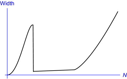
Figure 1: Schematic predicted behaviour of system width, i.e. length in the direction perpendicular to the $B_{z}=0$ line, as a function of electron number. The first critical number requires a full solution of the Hartree Fock equation but the asymptotic analysis leading to Eq.63 yields an estimate for the second one.

Only a full solution of the Hartree-Fock equations can reveal the true behavior but this must be deferred to some future time.

I  Preliminaries

The starting point is the 2-D Schrödinger equation describing free electrons confined within a rectangular $(L_{x},L_{y})$ sample. A $\hat{z}$-directed magnetic field increases linearly with $y$, $\ \vec{B}(y)=(0,0,yB^{\prime})$. The origin of coordinates is taken at the sample’s centre. With the inclusion of a Zeeman term the Hamiltonian is,

$$H=\frac{1}{2m}\left(\mathbf{p}-\frac{e}{c}\mathbf{A}\right)^{2}-\vec{\mu}\cdot\vec{B}.$$ (1)

The gauge potential is chosen to be independent of $x$,

$$\mathbf{A=}-\hat{x}\frac{1}{2}y^{2}B^{\prime}.$$ (2)

Since the Hamiltonian is invariant under translations of $x$, we have a plane wave solution, $\psi_{k}(x,y)=\frac{1}{\sqrt{L_{x}}}e^{-ik_{x}x}\varphi_{k_{x}}(y)$. The quantity $k_{x}$ is the eigenvalue of $\hat{p}_{x}=$ $\frac{\hslash}{i}\frac{\partial}{\partial x}$. Of course, $\hat{p}_{x}$ is not the canonical momentum operator and so $k_{x}$ is not the physical momentum. Translational invariance in $x$ allows imposition of periodic boundary conditions $\psi(x+L_{x},y)=\psi(x,y)$. The sum over $k_{x}$ is converted to an integral in the usual way,

$$N=\ \sum_{k_{x}}\longrightarrow\frac{L_{x}}{2\pi}\int_{k_{L}}^{k_{U}}dk_{x}\ =\frac{L_{x}}{2\pi}(k_{U}-k_{L})$$ (3)

Given relevant fundamental physical constants at this scale, together with the magnetic field gradient, a little experimentation leads to a unique definition of a length scale for the system,

$$L_{M}=\left(\frac{2\hslash c}{eB^{\prime}}\right)^{1/3}.$$ (4)

It is useful to define the dimensionless distance $\eta=y/L_{M}$ and wavenumber $\kappa=k_{x}L_{M}$ in terms of which,

$$N=\frac{1}{2\pi}\frac{L_{x}}{L_{M}}\sigma,\text{ \ \ }\sigma=\kappa_{U}-\kappa_{L}.$$ (5)

The effective potential for $y$-motion, to be inserted into the Schrodinger equation, is slightly asymmetric for electrons with spins parallel or antiparallel to the field,

$$\text{ }V(\eta,\kappa)=\frac{1}{2}(\eta^{2}-\kappa)^{2}\mp\frac{\lambda}{2}\eta\,.$$ (6)

Define $\alpha^{2}=\kappa$ for $\kappa>0$ and $\alpha^{2}=-\kappa$ for $\kappa<0$. The sign of $\kappa$ is crucial for determining the behavior of the eigenfunctions.  For $\kappa>0$ there are minima of the potential located at $\eta=\pm\alpha$. On the other hand, for $\kappa<0$ the two minima coalesce at $\eta=0.$ In both cases, for very large $\eta$ there is a quartic confining potential.

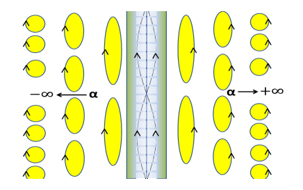
Figure 2: Schematic separation of regions for $\kappa>0$. In the center is the snake pit containing classical open (weaving) orbits. To the right ($\alpha>0$) and left ($\alpha<0$) electron orbits gradually close and asymptotically approach circular Landau orbits. For $\kappa<0$ there are no closed orbits.

For a typical gradient of 1 Gauss per $\mathring{A}$, $L_{M}\approx 1096$ $\mathring{A}$ that is attained in physical situations, and taking the effective electron mass $m^{\ast}\approx 0.068m_{e}$, the energy scale is set by $\varepsilon_{0}$,

$$\text{ }\varepsilon_{0}=\frac{\hslash^{2}}{m^{\ast}L_{M}^{2}}\approx 93.25\times 10^{-6}eV.$$ (7)

With the in-medium electron g-factor, the dimensionless Zeeman coupling constant $\lambda$ is,

$$\lambda=g^{\ast}\frac{m^{\ast}}{m}\approx 0.0272.$$ (8)

The Zeeman term is negligible for most purposes. But the symmetry of the double-well potential is broken in the presence of spin; only the slightest push suffices to send electrons over to one side or the other. One can readily work out the asymptotic wavefunction after expanding around the right well bottom for spins aligned along $\mathbf{B}$,

$$\varphi_{\alpha}=N\exp\left[-\alpha\sqrt{1-\frac{3\lambda}{4\alpha^{3}}}\left(\eta-\alpha+\frac{\lambda}{4\alpha^{2}}\right)^{2}\right].$$ (9)

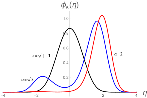
Figure 3: Rapid approach to asymptotia. Exact (numerical) solutions of the one-body equation with quartic term included. Convergence to asymptotic solution is achieved after only 2-3 magnetic lengths. Note also the strong influence which even the tiny Zeeman term exerts; without it the ground state wavefunction would be symmetrical at large $\alpha$.

For purposes of analysis we separate three crucial regions of $k_{x}$-space: the “snake-pit” $S$ at the centre, and left/right asymptotia,

$$\kappa_{a}<L<\kappa_{b},\text{ \ \ \ }\kappa_{b}<S<\kappa_{B}\text{, \ \ \ }\kappa_{B}<R<\kappa_{A}\text{\ .}$$ (10)

$S$ extends roughly 2-3 magnetic length units on either side. The classical orbits inside $S$ are open but they close in some complicated way as one moves outward towards $R$. For large $\kappa_{A}$, they tend towards becoming circles because the $B$ field varies less and less over the size of the orbit as compared to the value at the center. Quantum mechanically they eventually become $n=0$ Landau states. Fig.2 displays a numerical diagonalization of the Hamiltonian with the potential Eq.6. It shows that the approach to right asymptotia is extremely fast. With $\lambda=0$, $\varphi_{\kappa}(\eta)$ would be perfectly symmetric. Notwithstanding the tiny asymmetry of the double well potential (because of the smallness of $\lambda$ in Eq.8), we see that almost the entire wavefunction has moved to the right for $\kappa=4$, i.e. $\alpha=2.$ For $\kappa<<0$, the situation is still simpler for the lowest quantum state. From being only approximately Gaussian at $\kappa=0$, it becomes nearly perfect Gaussian as $\kappa$ moves further to the left. We see that non-Gaussian behavior is confined to near $S.$ Fortunately for the asymptotic analysis to be presented below, its contribution will be negligible for large $N$.

II Exchange Interaction

The starting point is the expression for the exchange energy,

$$E_{ex}=-\frac{e^{2}}{2\varepsilon_{D}}\int d^{2}rd^{2}r^{\prime}\frac{\rho(\mathbf{r,r}^{\prime})\rho(\mathbf{r}^{\prime}\mathbf{,r})}{\left|\mathbf{r}-\mathbf{r}^{\prime}\right|},$$ (11)

where,

$$\rho(\mathbf{r,r}^{\prime}) = \sum_{k_{x}}\psi_{k_{x}}^{\ast}(\mathbf{r)}\psi_{k_{x}}(\mathbf{r}^{\prime}\mathbf{)}$$ (12)

$$= \frac{1}{2\pi}\int_{k_{L}}^{k_{U}}dk_{x}e^{ik_{x}(x-x^{\prime})}\rho_{k_{x}}(y\mathbf{,}y^{\prime}).$$ (13)

The electron density is invariant in the $\hat{x}$ direction and so requires finite integration limits but in the $\hat{y}$ direction it tails off exponentially before reaching the sample edges. With integration regions explicitly indicated, the exchange integral becomes,

$$E_{ex} = -\frac{e^{2}}{2\varepsilon_{D}}\int d^{2}rd^{2}r^{\prime}\frac{\rho(\mathbf{r,r}^{\prime})\rho\mathbf{(r}^{\prime}\mathbf{,r})}{\sqrt{\mathbf{(}x\mathbf{-}x^{\prime})^{2}+\mathbf{(}y\mathbf{-}y^{\prime})^{2}}}$$ (15)

$$= -\frac{e^{2}}{2\varepsilon_{D}}\int_{-\frac{1}{2}L_{x}}^{\frac{1}{2}L_{x}}dxdx^{\prime}\int_{-\infty}^{\infty}dydy^{\prime}$$

$$\times\frac{e^{i(k-k^{\prime})(x-x^{\prime})}}{\sqrt{\mathbf{(}x\mathbf{-}x^{\prime})^{2}+\mathbf{(}y\mathbf{-}y^{\prime})^{2}}}\rho_{k_{x}}(y\mathbf{,}y^{\prime})\rho_{k_{x}}(y^{\prime}\mathbf{,}y).$$

Normalizing the energy below in units of $\frac{\hslash^{2}}{m^{\ast}L_{M}^{2}}$ and converting all quantities in to corresponding dimensionless variables, the energy functional becomes,

$$\mathcal{E[}\varphi_{\kappa}^{\ast},\varphi_{\kappa}] = \int_{\kappa_{L}}^{\kappa_{U}}d\kappa\int_{-\infty}^{\infty}d\eta\varphi_{\kappa}^{\ast}\left(-\frac{1}{2}\frac{d^{2}}{d\eta^{2}}+V\right)\varphi_{\kappa}$$ (16)

$$-\mu\int_{\kappa_{L}}^{\kappa_{U}}d\kappa d\kappa^{\prime}\int_{-l_{x}/2}^{l_{x}/2}d\xi d\xi^{\prime}\int_{-\infty}^{\infty}d\eta d\eta^{\prime}$$

$$\times\rho_{\kappa}(\eta\mathbf{,}\eta^{\prime})\rho_{\kappa^{\prime}}(\eta^{\prime}\mathbf{,}\eta)\frac{e^{i(\kappa-\kappa^{\prime})(\xi\mathbf{-}\xi^{\prime})}}{\sqrt{\mathbf{(}\xi\mathbf{-}\xi^{\prime})^{2}+\mathbf{(}\eta\mathbf{-}\eta^{\prime})^{2}}},$$

where the sample’s length (in units of magnetic length) is $l_{x}=L_{x}/L_{M}$ and $\mu$ is the exchange coupling,

$$\mu=\frac{e^{2}m^{\ast}}{8\pi^{2}\varepsilon_{D}\hslash^{2}}L_{M}=\frac{1}{8\pi^{2}}\frac{L_{M}}{a_{B}^{\ast}},$$ (17)

with $a_{B}^{\ast}=\varepsilon_{D}\hslash^{2}/e^{2}m^{\ast}$ being the in-medium Bohr radius. For the typical values discussed above, $\mu\approx$ $0.137$. To get the equation of motion, Eq.16 must be minimized with respect to $\varphi_{\kappa}^{\ast}(\eta)$. Adding in a Lagrange multiplier constraint to keep $\varphi$ normalized gives the equation of motion,

$$\left(-\frac{1}{2}\frac{d^{2}}{d\eta^{2}}+V(\eta)-\frac{\lambda}{2}\eta\right)\varphi=\int_{\kappa_{L}}^{\kappa_{U}}d\kappa^{\prime}\int_{-\infty}^{\infty}d\eta^{\prime}$$

$$\times\int_{-l_{x}/2}^{l_{x}/2}d\xi d\xi^{\prime}\frac{e^{i(\kappa-\kappa^{\prime})(\xi\mathbf{-}\xi^{\prime})}}{\sqrt{\mathbf{(}\xi\mathbf{-}\xi^{\prime})^{2}+\mathbf{(}\eta\mathbf{-}\eta^{\prime})^{2}}}\rho_{\kappa^{\prime}}(\eta^{\prime}\mathbf{,}\eta)\varphi_{\kappa}(\eta^{\prime})$$

$$=\varepsilon_{HF}\varphi_{\kappa}(\eta).$$ (18)

The integration limits must be determined separately. For this we must keep fixed the electron number while minimizing the total energy function which takes the generic form,

$$\mathcal{E[}\varphi_{\kappa}^{\ast},\varphi_{\kappa}]=\int_{\kappa_{1}}^{\kappa_{2}}\varepsilon(\kappa)d\kappa-\mu\int_{\kappa_{1}}^{\kappa_{2}}\int_{\kappa_{1}}^{\kappa_{2}}d\kappa d\kappa^{\prime}g(\kappa,\kappa^{\prime}).$$ (19)

Using a Lagrange multiplier to enforce the number constraint $\kappa_{2}-\kappa_{1}=\sigma$ gives the additional condition,

$$\varepsilon(\kappa_{2})-\varepsilon(\kappa_{1})-2\mu\int_{\text{$\kappa$}_{1}}^{\text{$\kappa$}_{2}}d\text{$\kappa$}\left[g(\text{$\kappa$}_{2},\text{$\kappa$})-g(\text{$\kappa$}_{1},\text{$\kappa$})\right]\,=0.$$ (20)

This is an infinite set of coupled non-linear integrodifferential equations that must be brought into some tractable form. To solve this numerically - by iteration of course - a basis set of functions will be needed, the choice of which will be quite crucial. One clearly needs to develop intuition if the system is to be solved numerically. The goal here is to explore whether some analytical results can be derived and used to illuminate these fairly opaque equations.

III Effective Potential

For systems that can be presumed to be infinite, translational invariance can make calculation of fermion exchange effects tractable because the simplicity of the single particle wavefunctions is maintained even in the presence of two-body interactions. Hence, upon making a suitable gauge choice, first order exchange corrections can be calculated for electron Landau levels in a uniform magnetic field. But in the system under consideration here, no translational invariance exists perpendicular to the axis of zero $B$. Hence if one starts from a solution of the single particle Schrodinger equation where the potential experienced by an electron owes entirely to the external magnetic field, one expects that turning on the Coulomb interaction between electrons would drastically change the single particle wavefunctions. This would be especially true in a system where the Coulomb exchange energy can be many times larger than the energy originating from kinetic and confining terms in the single particle Hamiltonian, as indeed does happen for the system under consideration. It was therefore interesting to see the emergence of simplicity in an asymptotic limit.

First consider large positive $\kappa=\alpha^{2}$, i.e. far to the right of the snake pit and only electrons in the range $\alpha_{B}<$ $\alpha<$ $\alpha_{A}$.  Interactions with electrons with the $S$ and $L$ regions are excluded; they are in fact exponentially suppressed. For spins aligned along the magnetic field the equation determining $\varphi_{\alpha}$ is,

$$\left(-\frac{1}{2}\frac{d^{2}}{d\eta^{2}}+V\right)\varphi_{\alpha}(\eta)$$ (21)

$$= 4\mu\int_{\alpha_{B}}^{\alpha_{A}}\frac{\alpha^{\prime}}{\alpha}d\alpha^{\prime}\int_{-\infty}^{\infty}d\eta^{\prime}\int_{-l_{x}/2}^{l_{x}/2}d\xi d\xi^{\prime}$$

$$\times\rho_{\alpha^{\prime}}(\eta^{\prime}\mathbf{,}\eta)\varphi_{\alpha}(\eta^{\prime})\frac{e^{i(\alpha^{2}-\alpha^{2\prime})(\xi\mathbf{-}\xi^{\prime})}}{\sqrt{\mathbf{(}\xi\mathbf{-}\xi^{\prime})^{2}+\mathbf{(}\eta\mathbf{-}\eta^{\prime})^{2}}}.$$

In principle every electron between $\alpha_{B}$ and$\ \alpha_{A}$ interacts with every other one, a manifestation of the non-local interaction of the exchange potential. However, in the $\alpha\rightarrow\infty$ a series of approximations reduces the above to a relatively simple local form. Qualitatively there are two reasons for this. First, at large $\alpha$ (in the absence of exchange), the free wavefunctions are narrowly peaked Gaussians. Thus an electron located at $\alpha$ will have exponentially small overlap with another at $\alpha^{\prime}$ unless the two points are close to each other. Hence what is non-local can hopefully be modeled with a local potential that emerges naturally from Eq.21  in some approximate way. Second, the exchange interaction in 2-D is attractive and peaks strongly at $\alpha=\alpha^{\prime}$ thus encouraging electrons to come closer to each other. These qualitative considerations will be made quantitative below.

As a first step, expand the potential about the well bottom located to the right at $\alpha-\lambda/8\alpha^{2}+$ $O(\lambda^{2}).$ The smallness of $\lambda$ means the well bottom can be safely assumed to be at $\alpha$ for large positive $\alpha$. After changing variables to $w$,

$$w=\sqrt{\alpha}(\eta-\alpha),\text{ \ }\beta=\alpha-\alpha^{\prime}.$$ (22)

Eq.21 can be reexpressed as,

$$\left(-\frac{1}{2}\frac{d^{2}}{dw^{2}}+2w^{2}-\varepsilon_{HF}\right)\varphi_{\alpha}(w)$$ (23)

$$= \mu\int_{\alpha-\alpha_{A}}^{\alpha-\alpha_{B}}d\beta h_{\alpha}(\beta)\varphi_{\alpha-\beta}(w),$$

where,

$$h_{\alpha}(\beta) = 4\frac{\alpha^{\prime}}{\alpha}\int_{-l_{x}/2}^{l_{x}/2}d\xi d\xi^{\prime}\int_{-\infty}^{\infty}d\eta^{\prime}$$ (24)

$$\times\frac{\varphi_{\alpha^{\prime}}^{\ast}(\eta^{\prime})\varphi_{\alpha}(\eta^{\prime})e^{i(\alpha^{2}-\alpha^{2\prime})(\xi\mathbf{-}\xi^{\prime})}}{\sqrt{\mathbf{(}\xi\mathbf{-}\xi^{\prime})^{2}+\mathbf{(}\eta\mathbf{-}\eta^{\prime})^{2}}}$$

$$= 8\frac{\alpha^{\prime}}{\alpha}\int_{0}^{l_{x}}dt\int_{0}^{t}ds\int_{-\infty}^{\infty}du$$

$$\times\frac{\varphi_{\alpha-\beta}^{\ast}(\eta^{\prime})\varphi_{\alpha}(\eta^{\prime})}{\sqrt{s^{2}+u^{2}}}e^{i(2\alpha-\beta)\beta s}$$

In going from Eq.23 to Eq.24, new variables $t,s,u$ have been defined,

$$\xi=t+\frac{1}{2}s,\ \ \xi^{\prime}=t-\frac{1}{2}s,\text{ \ }\eta\mathbf{\ -}\eta^{\prime}\ =u.$$ (25)

and the change in the shape of the ($\xi,\xi^{\prime})$ integration plane has been included.

$$\int_{-l_{x}/2}^{l_{x}/2}d\xi d\xi^{\prime}f(\left|\xi-\xi^{\prime}\right|)\rightarrow 2\int_{0}^{l_{x}}dt\int_{0}^{t}dsf(\left|s\right|).$$ (26)

The integral over $\eta^{\prime}$or, equivalently over $u$, can be extended to infinity if the electrons are assumed to form a self-binding system and $\varphi(\pm\infty)=0$. However, because of translational invariance, one cannot assume the same here in $x$. This will, as we shall see, has profound consequences.

At this point we shall assume that the integrand in Eq.24 is significant only when $\beta<<\alpha$, i.e. two narrowly peaked wavefunctions must nearly coincide to give a non-zero contribution. This will lead to consistent results that can be verified after the calculation is performed. As a first guess we use the lowest order solution of the free $\mu=0$ equation which, at leading order, yields for the product of two wavefunctions,

$$\varphi_{\alpha-\beta}^{(0)}(\eta^{\prime})\varphi_{\alpha}^{(0)}(\eta^{\prime})=\sqrt{\frac{2\alpha}{\pi}}e^{-\frac{1}{2}\alpha\beta^{2}}e^{-2\alpha\left(u+\frac{w}{\sqrt{\alpha}}-\frac{1}{2}\beta\right)^{2}}.$$ (27)

The integrals in Eq.24 cannot be done exactly. Since $\alpha$ is a large parameter one can take recourse to the method of stationary phase, followed by steepest descent. Transforming to polar coordinates,

$$u=\rho\cos\theta,\text{ \ }s=\rho\sin\theta,$$ (28)

with $0<\theta<2\pi$ and $0<\frac{t}{\left|\sin\theta\right|}<\rho<\infty$ gives,

$$h_{\alpha}(\beta) = 8\int_{0}^{l_{x}}dt\int_{0}^{t}ds\int_{-\infty}^{\infty}du$$ (31)

$$\times\frac{\varphi_{\alpha-\beta}^{(0)\ast}(\eta^{\prime})\varphi_{\alpha}^{(0)}(\eta^{\prime})}{\sqrt{s^{2}+u^{2}}}e^{i(2\alpha-\beta)\beta s}$$

$$= 4\sqrt{2\alpha}e^{-\frac{1}{2}\alpha\beta^{2}}\int_{0}^{l_{x}}dt\int_{0}^{t}d\rho d\theta$$

$$\times e^{-2\alpha\left(\rho\cos\theta+\frac{w}{\sqrt{\alpha}}-\frac{1}{2}\beta\right)^{2}}e^{i2\alpha\beta\rho\sin\theta}$$

$$= 32\sqrt{2}\pi e^{-w^{2}}e^{-\alpha\left(\beta-\frac{w}{\sqrt{\alpha}}\right)^{2}}$$

$$\times\int_{0}^{l_{x}}dt\int_{0}^{t}d\rho\frac{\sin(2\alpha\beta\rho+\pi/4)}{\sqrt{\beta\rho}}.$$

In going from Eq.31 to Eq.31 just the leading term have been kept, and in going from Eq.31 to Eq.31 it was recognized that the phase becomes stationary at $\theta=\pi/2,3\pi/2$. Anticipating that $\beta$ will also be integrated upon later, and noting the smooth behavior of the remaining integrals, we can further simplify $h_{\alpha}(\beta)$ by replacing $\beta\rightarrow w/\sqrt{\alpha}$ in the integrand,

$$h_{\alpha}(\beta) = 32\sqrt{2\alpha}\pi\frac{e^{-w^{2}}}{\sqrt{\left|w\right|}}e^{-\alpha\left(\beta-\frac{w}{\sqrt{\alpha}}\right)^{2}}$$ (32)

$$\times\int_{0}^{l_{x}}dt\int_{-t}^{t}d\rho\frac{\sin(2\alpha\beta\rho+\pi/4)}{\sqrt{\beta\rho}}.$$

The last two integrals can be performed exactly in terms of Fresnel integrals $C(\sqrt{\alpha}l_{x}w)$ and $S(\sqrt{\alpha}l_{x}w)$ but the results are not illuminating and will not be displayed here. Two limiting cases suffice to make the point below,

We can insert Eq.31 into Eq.23 and keep just the first term in the expansion about $\beta=0$. The remaining integral is trivially done and we see the promised result, an approximate effective potential determining $\varphi_{\alpha}$,

$$\left(-\frac{1}{2}\frac{d^{2}}{dw^{2}}+2w^{2}+\mathcal{V}(w)\right)\varphi_{\alpha}=\varepsilon_{HF}\varphi_{\alpha},$$ (33)

where the limiting cases for $\mathcal{V}(w)$ can easily be worked out,

$$\mathcal{V}(w)=\left\{\begin{array}[]{lr}-\frac{32\pi^{2}}{\sqrt{\alpha}}l_{x}\frac{e^{-w^{2}}}{\left|w\right|}&\left|w\right|>>\frac{1}{\sqrt{\alpha}l_{x}}\\ \begin{array}[]{l}-\frac{128}{3}\frac{\sqrt{2\pi^{3}}}{\alpha^{1/4}}l_{x}^{3/2}\\ \times(1+\frac{2}{5}\sqrt{\alpha}wl_{x}-\frac{6}{35}\alpha w^{2}l_{x}^{2})\end{array}&\left|w\right|<<\frac{1}{\sqrt{\alpha}l_{x}}\end{array}\right..$$ (34)

Observe that: a)$\mathcal{V}(w)$ has a much shorter range relative to $2w^{2}$and so electrons confined by the potential well produced by the magnetic field are unaffected at longer distances, b)$\mathcal{V}(w)$ is attractive and has the effect of further narrowing the wavefunction, c)$\mathcal{V}(w)\rightarrow 0$ as $\alpha\rightarrow\infty$ and so the exchange interaction vanishes asymptotically, d)$\mathcal{V}(w)$ depends on $l_{x}$, i.e. the length of the sample in the $x$ direction as measured in magnetic length units. This last point is somewhat surprising. We have argued for near locality in $y$ but linear dependence upon $l_{x}$ shows strong non-locality in $x$. Electrons at different $x$ positions are definitely communicating much more with each other than with those which are located perpendicular to the $B=0$ line. At one level this can be understood from the $x$-independence of the electron density which follows from translational invariance.

As a qualitative confirmation, one can insert a trial Gaussian $\psi=Ne^{-cw^{2}}$with $c$ a variational parameter into the first order perturbation energy,

$$\varepsilon(c)=\int_{-\infty}^{\infty}\left(\frac{1}{2}\psi^{\prime 2}+\psi(2w^{2}+\mathcal{V})\psi\right)dw.$$ (35)

Unfortunately the integrations are analytically too complex to be useful, but for typical parameter values numerical integration can be readily done. The essential point is that $\varepsilon(c)$ achieves a minimum at $c=c_{\min}>1$ for $\alpha>>1$ and that $c\rightarrow 1$ as $\alpha\rightarrow\infty$. This tells us that the wavefuncton gets even more peaked at finite $\alpha$ and that the small $\beta$ assumption made earlier was indeed valid.

So far we have concentrated upon the right asymptotic region. Similar conclusions will be drawn for the left asymptotic region: one again recovers the free solution for $\kappa\rightarrow-\infty$, the exchange potential leads to narrowing of wavefunctions, and for large enough $l_{x}$ the exchange energy is again proportional to $l_{x}$. However these conclusions will be based upon the analysis presented in the next section where the reasoning will take into account the very different physics: there is only a single well for negative $\kappa$ instead of two wells for positive $\kappa.$

To conclude this section: the exchange term involves a six dimensional integral that was dealt with here in a limiting case only. The results achieved will, however, be useful in attempting a full and unconstrained self-consistent calculation.

IV Asymptotic Energy

Armed with the knowledge that the asymptotic solution is the $\mu=0$ solution - and that this will be approached for sufficiently large $\alpha$ - we now calculate the action to leading order in the right and left asymptotic regions.

IV.1 Right Region

The energy functional in the right asymptotic region is:

$$\mathcal{E}^{R} = \int_{\alpha_{B}}^{\alpha_{A}}2\alpha d\alpha\int_{-\infty}^{\infty}d\eta$$ (37)

$$\times\varphi_{\alpha}^{(0)}\left({\small-}\frac{1}{2}\frac{d^{2}}{d\eta^{2}}+2\alpha^{2}(\eta-\alpha)^{2}\right)\varphi_{\alpha}^{(0)}$$

$$\mathcal{E}_{ex}^{RR} = -\mu\int_{\alpha_{B}}^{\alpha_{A}}4\alpha\alpha^{\prime}d\alpha d\alpha^{\prime}\int_{-l_{x}/2}^{l_{x}/2}d\xi d\xi^{\prime}\int_{-\infty}^{\infty}d\eta d\eta^{\prime}$$ (38)

$$\times\rho_{\alpha}^{(0)}(\eta\mathbf{,}\eta^{\prime})\rho_{\alpha}^{(0)}(\eta^{\prime}\mathbf{,}\eta)\frac{e^{i(\alpha^{2}-\alpha^{2\prime})(\xi\mathbf{-}\xi^{\prime})}}{\sqrt{\mathbf{(}\xi\mathbf{-}\xi^{\prime})^{2}+\mathbf{(}\eta\mathbf{-}\eta^{\prime})^{2}}}.$$

Here $\varphi_{\alpha}^{(0)}(\eta)=N\exp[-\alpha(\eta-\alpha)]$ is the free solution and $\mathcal{E}^{R}$ is trivially calculated,

$$\mathcal{E}^{R}=\frac{2}{3}(\alpha_{{}_{U}}^{3}-\alpha_{{}_{L}}^{3}).$$ (39)

However, even with the simple displaced Gaussian, the six-dimensional integral is non-trivial because only two of the six integration have limits that can be pushed off to infinity. However a remarkably simple analytic result can be extracted in the large $\alpha$ limit, $1<<\alpha_{B}<\alpha<$ $\alpha_{A}$. It is displayed below in Eq.47. Arriving at the result will need a sequence of steps beginning with a transformation to more appropriate coordinates:

$$\xi = t+\frac{1}{2}s,\ \ \xi^{\prime}=t-\frac{1}{2}s,\ \eta=\text{v}+\frac{1}{2}u,\text{ }$$ (40)

$$\eta^{\prime} = \text{v}-\frac{1}{2}u,\text{ \ }\alpha=\gamma+\frac{1}{2}\beta,\text{ \ }\alpha^{\prime}=\gamma-\frac{1}{2}\beta.$$ (41)

Next, we suitably arrange terms in the integrand in Eq.38 and perform the integrals over $u$,v (whose integration limits extend to infinity in both directions). After some algebra and using $\gamma>>\beta$, four integrations remain:

$$\mathcal{E}_{ex}^{RR} = -\mu\int d\gamma d\beta\int dtds\frac{4}{\sqrt{\pi}}\gamma^{5/2}$$ (42)

$$\times e^{-\gamma(\beta^{2}-\frac{1}{2}s^{2})+i2\gamma\beta s}K_{0}(\tfrac{1}{2}\gamma s^{2}).$$

$K_{0}$ is the modified Bessel function. For any even function $g(\gamma,\beta)=g(\gamma,-\beta)$ integrated over the $\alpha,\alpha^{\prime}$ integration region as indicated in Eq.38 one can readily show,

$$\int d\gamma d\beta g(\gamma,\beta)\rightarrow\frac{1}{2}\int_{0}^{\alpha_{A}-\alpha_{B}}d\gamma\int_{-\gamma}^{\gamma}d\beta$$

$$\times\left[g(\frac{1}{2}\gamma+\alpha_{B},\beta)+g(-\frac{1}{2}\gamma+\alpha_{A},\beta)\right]$$ (43)

Consider now the integrals are over $\beta,s.$ The $\beta$ integration may be safely extended to infinity since the only support comes from the $\beta\approx 0$ region but the $s$ integration limits are finite. Transform to polar coordinates $\beta=\rho\cos\theta,$  $s=\rho\sin\theta$ and $0<\theta<2\pi$ and $0<\frac{t}{\left|\sin\theta\right|}<\rho<\infty.$ In this domain the phase is stationary at $\theta=\pm\frac{\pi}{4},\pm\frac{3\pi}{4}.$ Adding contributions in the $\theta$ integration from all 4 points yields,

$$\int d\beta ds \rightarrow \frac{4}{\sqrt{\pi}}\gamma^{5/2}\int d\rho d\theta e^{-\frac{1}{4}\gamma\rho^{2}(1+3\cos 2\theta)}$$ (45)

$$\times e^{i\gamma\rho^{2}\sin 2\theta}K_{0}(\tfrac{1}{2}\gamma\rho^{2}\sin^{2}\theta)$$

$$= 16\pi\gamma^{2}\int_{0}^{\sqrt{2}t}d\rho e^{-\frac{1}{4}\gamma\rho^{2}}K_{0}(\tfrac{1}{4}\gamma\rho^{2})$$

$$\times\left(\sin\gamma\rho^{2}+\cos\gamma\rho^{2}\right)$$

The above integral has no analytic form for finite $t$. However for large enough $l_{x}$ and $\gamma\rightarrow\infty$ (which is the same thing as large $\alpha$ because $\gamma=(\alpha+\alpha^{\prime})/2$ and both $\alpha^{\prime}$s are large)  we can use,

$$\int_{0}^{\infty}dxe^{-(1-4i)x^{2}}K_{0}(x^{2})=\sqrt{\frac{\pi}{2}}K(2i),$$ (46)

where $K$ is the elliptic integral of the first kind (not to be confused with the Bessel function $K_{0}$) and $K(\pm 2i)=1.236\pm 0.389i$ . The remaining integrals on $t$ and $\gamma$ are now trivially done to yield the final result for the exchange contribution of electrons in the right asymptotic region,

$$\mathcal{E}_{ex}^{RR} = -\mu l_{x}C(\alpha_{A}-\alpha_{B})^{5/2},$$ (47)

$$C = \frac{16}{5}\sqrt{2}\pi^{3/2}(1+i)(K(-2i)-iK(2i))$$

$$= 81.8977.$$

Again, note that the exchange energy is proportional to $l_{x}$ for large enough $l_{x}$. Also, $\mathcal{E}_{ex}^{RR}\sim$ $\alpha_{A}^{5/2}{}$ grows less rapidly than $\mathcal{E}_{sp}^{R}\sim\alpha_{{}_{A}}^{3}$ . This will be crucial when we consider the system’s stability.

IV.2 Left Region

Next, consider the energy functional in the left asymptotic region. While there is a small risk of confusion with the notation used above for the right asymptotic region, we shall nevertheless continue to use below the symbols $\alpha,\kappa$ but with a crucial change of sign. In the following $\alpha^{2}=-\kappa>0$ is assumed large with $\alpha_{a}>\alpha_{b}>>1$,

$$\mathcal{E}^{L} = \int_{-\kappa_{a}}^{-\kappa_{b}}d\kappa\int_{-\infty}^{\infty}d\eta$$ (50)

$$\times\varphi_{\alpha}^{\ast}\left(-\frac{1}{2}\frac{d^{2}}{d\eta^{2}}+\frac{1}{2}(\eta^{2}+\alpha^{2})^{2}\right)\varphi_{\alpha}$$

$${\small\approx} \int_{\alpha_{b}}^{\alpha_{a}}2\alpha d\alpha\int_{-\infty}^{\infty}d\eta$$ (52)

$$\times\varphi_{\alpha}^{\ast}\left(-\frac{1}{2}\frac{d^{2}}{d\eta^{2}}+\eta^{2}\alpha^{2}+\frac{1}{2}\alpha^{4}\right)\varphi_{\alpha}{\small.}$$

In the quadratic approximation the lowest eigenfunction $\varphi_{\alpha}^{(0)}(\eta)=Ne^{-\alpha\eta^{2}/\sqrt{2}}$ leads to

$$\mathcal{E}^{L}=\frac{1}{6}(\alpha_{a}^{3}-\alpha_{b}^{3})\left(\alpha_{a}^{3}+\alpha_{b}^{3}+3\right).$$ (53)

The Coulomb exchange energy is exactly as in Eq.38 with new integration limits $\alpha_{A}\rightarrow\alpha_{a}$ and $\alpha_{B}\rightarrow\alpha_{b}.$ However physically this is a very different physical regime where backward moving electrons are clustered along the $B_{z}=0$ line. Using and using $\gamma>>\beta$ and performing the two indicated integrations with infinite limits yields,

$$\mathcal{E}_{ex}^{LL} = -\frac{4}{\sqrt{\pi}}\mu\int d\gamma d\beta\int dtds\gamma^{5/2}e^{\frac{1}{2}s^{2}\gamma}$$ (54)

$$\times K_{0}(\frac{1}{2}s^{2}\gamma)\cos(2\beta\gamma s)$$

All integrals in Eq.54 have finite limits. However in the limit of both large $\gamma$ and $l_{x}$ a careful analysis shows that the $s$-integration limits can be pushed to infinity, giving a result in terms of a Meijer G hypergeometric function,

$$\mathcal{E}_{ex}^{LL}=-\mu\frac{1}{\sqrt{\pi}}\int_{0}^{\alpha_{a}-\alpha_{b}}\gamma^{3/2}d\gamma$$

$$\times\int_{-\gamma}^{\gamma}d\beta\left[g(\frac{1}{2}\gamma+\alpha_{B},\beta)+g(-\frac{1}{2}\gamma+\alpha_{A},\beta)\right]$$ (55)

$$g(\gamma,\beta)=G_{2,3}^{2,2}\left(\beta^{2}\gamma\left|\begin{array}[]{c}1,1\\ \frac{1}{2},\frac{1}{2},0\end{array}\right.\right).$$ (58)

In the the large $\gamma$ limit, $g(\gamma,\beta)\rightarrow$ $\pi\log(16\beta^{2}\gamma)+\pi\boldsymbol{\gamma_{E}}$  where $\boldsymbol{\gamma_{E}}$  is Euler-Mascheroni constant, $\boldsymbol{\gamma_{E}}=0.57721$. Carrying out the remaining integrations yields the final result for $\alpha_{A}>\alpha_{B}>>1,$

$$\mathcal{E}_{ex}^{LL} = -\mu l_{x}\alpha_{a}^{5/2}(c_{a}+c_{b}\log\alpha_{a})$$ (59)

$$c_{a} = \frac{4\sqrt{\pi}(-92+35\sqrt{2}+30\boldsymbol{\gamma}+240\log 2-60\coth^{-1}\sqrt{2})}{75}$$

$$c_{b} = \frac{4}{75}\sqrt{\pi}$$

Comparing Eq.59 to Eq.47 we note that both are proportional to $\alpha^{5/2}$ (albeit the $\alpha^{\prime}s$ refer to different physical quantities) but that there is an additional logarithmic dependence in the negative $\kappa$ case.

One issue deserves further consideration before we move on. What justifies using $\varphi_{\alpha}^{(0)}(\eta)=Ne^{-\alpha\eta^{2}/\sqrt{2}}$ for large $\alpha$ in the left asymptotic region? Instead of following the line of argument used earlier, we shall use the variational principle. To this end, we take as trial wavefunction $\psi\sim e^{-\alpha\xi\eta^{2}/\sqrt{2}}$ with $\xi$ a variational parameter. Inserting this, and going the same sequence of steps leading to Eq.59, the energy takes the following schematic form,

$$\mathcal{E}\sim\alpha_{a}^{3}\left(d+\frac{1}{d}\right)-k\alpha_{a}^{5/2}\sqrt{d},$$ (60)

where crucially $k>0$ and its precise value can be read off from Eq.59. For sufficiently large $\alpha_{a}$ the minimum is attained at $d=1+k\alpha_{a}^{-1/2}/4$. Thus the Gaussian becomes progressively more peaked as one moves from infinity inwards. This confirms for $\kappa\rightarrow-\infty$ what we had seen earlier for $\kappa\rightarrow+\infty.$

V Stability/ Instability

A 2-D electron gas in a linearly rising magnetic field in the absence of the exchange force, i.e. $\mu=0$, will increase its width monotonically as electrons are added. The condition Eq.20 gives $\varepsilon(\kappa_{2})=\varepsilon(\kappa_{1})$ or, $\frac{1}{2}\alpha_{a}^{4}=\alpha_{A}$ subject to the number conservation constraint $\alpha_{A}^{2}+\alpha_{a}^{2}=\sigma=2\pi L_{M}\frac{N}{L_{x}}.$ This always has a solution. But now imagine we add electrons one by one. They will, of course, go into the lowest quantum state and first fill up the snake pit before expanding eventually into the left/right asymptotic regions. This determines the “Fermi surface” for the system, i.e. the placement of single electrons into single particle states.

Now turn on the exchange interaction. Keeping $\alpha_{b}$ and $\alpha_{A}$ fixed at some low values we are interested in the limit where $\alpha_{a},\alpha_{A}$ are in their respective asymptotic regions. With the cautionary note that the goal is to expose the essential physics rather than do a quantitative calculation, we shall go so far in asymptotia that only the extreme left and right regions are relevant. Overlaps between different regions then become negligible. Keeping only leading terms, subject to $\alpha_{A}^{2}+\alpha_{a}^{2}=\sigma,$ the question becomes whether the approximated energy,

$$\mathcal{E}=\frac{1}{6}\alpha_{a}^{6}+\frac{2}{3}\alpha_{{}_{A}}^{3}-\mu l_{x}(C\alpha_{A}^{5/2}+c_{a}\alpha_{a}^{5/2})$$ (61)

has a minimum. To eliminate the constraint, put $\alpha_{a}=\sqrt{\sigma}\sin\theta,$ $\alpha_{A}=\sqrt{\sigma}\cos\theta.$ Since $\alpha_{A}>>\alpha_{a}$ the last term in Eq.61 can be dropped. Thus,

$$\mathcal{E}=\frac{1}{6}\sigma^{3}\sin^{6}\theta+\frac{2}{3}\sigma^{3/2}\cos^{3}\theta-\mu l_{x}C\sigma^{5/4}\cos^{5/2}\theta$$ (62)

Minimizing this with respect to $\theta$,

$$\sin^{4}\theta=\frac{2}{\sigma^{3/2}}\cos\theta-\frac{5}{2\sigma^{7/4}}\mu l_{x}C\sqrt{\cos\theta},$$ (63)

together with positivity of the second derivative ($C$ is defined in Eq.IV.1). For $\mu=0\$and$\ \ \sigma\rightarrow\infty$, at leading order $\theta=2^{1/4}\sigma^{-3/8}$ and $\mathcal{E}^{\prime\prime}$ $\sim 2\sigma^{-9/2}>0.$ But for finite $\mu$ the condition for the system to become stable is,

$$1>\cos\theta>\frac{25}{32\sigma^{1/2}}\mu^{2}l_{x}^{2}C^{2},$$ (64)

or approximately that,

$$\sigma^{1/4} > \frac{5}{4\sqrt{2}}\mu l_{x}C\text{, or,}$$

$$2\pi L_{M}\frac{N}{L_{x}} > \left(\frac{5C}{32\sqrt{2}\pi^{2}}\frac{L_{x}}{a_{B}^{\ast}}\right)^{4}.$$ (65)

With this condition $\mathcal{E}^{\prime\prime}>0$ and so stability is assured.  For the system to resume expansion upon adding more electrons, the condition derived is $L_{M}N>c$ where $c$ is some constant that does not depend on either $N$ or $B$. Since $L_{M}\sim B^{-1/3}$, it follows that we must either increase $N$ or decrease $B$ to achieve the same $c$.

A by-product of the above analysis is that we can simply read off how the system size would increase with $N$ if exchange was absent,

$$\left\langle L_{y}\right\rangle=2^{1/4}\sigma^{1/8}L_{M}=\left(8\pi L_{M}\frac{N}{L_{x}}\right)^{1/8}L_{M}.$$ (66)

In Eq.66 $\left\langle L_{y}\right\rangle$ is equal to half the system’s width, i.e. the distance from the $B_{z}=0$ line to the last occupied state on the right (labeled by $\alpha_{a}$) provided: a)the sample boundary lies even further to the right, b)the exchange interaction is negligible $(\mu=0)$, c)$N$ is large enough so that the snake-pit is irrelevant.

VI Discussion

With $L_{x}=$1cm $\approx 10^{5}L_{M}$ for a 1 Gauss/$\mathring{A}$  gradient and the physical constants specified earlier, the condition from Eq.65 is $\sigma^{1/4}>9\times 10^{5}$ which corresponds to $N\sim 1.3\times 10^{10}$. To put this in context, note that in high mobility molecular-beam-epitaxially grown GaAs-AlGa heterostructures using electron beam lithography, electron densities are typically around $10^{11}$cm${}^{-2}.$ This suggests that an experimental check may not be too difficult.

The instability discussed in this paper can be understood using some hand-waving arguments. Far from the snake pit, each electron is in a locally constant $B$ field and hence approaches the characteristic motion of an electron in its lowest Landau level with a $B$ equal to that at the center of gyration. Because of the Pauli principle, it would appear that the double well always requires a system with more electrons to be larger. But let’s recall that that the kinetic-magnetic energy (positive) is proportional to the one-body density matrix $\rho$ while the exchange energy (negative) is proportional to $\rho^{2}.$ So, loosely speaking, as one adds electrons and increases the density, an electron acquires more neighbors. With the Pauli principle allowing only one electron in the state labeled by $\alpha$, the kinetic-magnetic term grows as $\alpha^{3}\sim y^{3},$ i.e. as the cube of the system’s width. The exchange energy grows somewhat more slowly as $\alpha^{5/2}$ and so, independent of the coefficient in front of it, will eventually become sub-dominant. The catch, however, is that the electron-electron effective coupling is large and so at some point it becomes energetically favorable for electrons to bunch together. That leads to collapse, i.e. the width decreases as $N$ increases. However, a further increase of $N$ eventually causes the kinetic-magnetic term to win and thus the system will resume expanding (until such time as it hits the boundary, which is excluded here).

Several interesting issues could be investigated at a later time. Obviously, the first is to set up the computational machinery for solving the Hartree-Fock equations whose solutions alone can give a definite value for when the first discontinuity occurs. The most suitable basis set for solving the HF equation is to take a set of simple harmonic oscillator functions that is not centered at $\eta=0$ but, instead, moves with the peak of the wavefunction and so is centered  close to $\eta=\alpha$ (see Fig.3). Of course one must compute overlaps between wavefunctions centred at different points and that brings in its own set of complications when calculating the 6-dim exchange integral. However a preliminary investigation shows it is likely to work efficiently.

One also needs to understand better the dependence of the coupling on $L_{x}$ and whether the periodic boundary conditions properly model the physical situation. Naively one should be able to push off the $x$-boundary to infinity because the Coulomb potential falls off with distance. However it does not fall off fast enough and so there is communication between electrons at roughly the same horizontal distance as the electrons near the sample’s edges. The resulting coupling is linear in $L_{x}$ only in the $L_{x}\rightarrow\infty$ limit; at finite size there appear to be Fresnel-like oscillations.

A separate question is what happens when the system expands to the horizontal boundary. While fairly trivial in the absence of exchange forces, it too could bring some surprises as the forces at the boundary push electrons into higher Landau levels and skipping states. Finally: what happens to gauge dependence? It is perfectly valid to work consistently within a single gauge (as done here) and calculate physical quantities. But, in principle, one should be able to make a different gauge choice and show that the same physical quantities emerge.

References

- (1) Quantum many particle systems, John W.Negele and Henri Orland, Addison Wesley, 1988.
- (2) Quantum theory of the electron liquid, Gabriele Giuliani and Giovanni Vignale, Cambridge University Press, 2005.
- (3) Effect of a non-uniform magnetic field on a two-dimensional electron gas in the ballistic region, J.E.Muller, Phys.Rev.Lett. 68, p385 (1992).
- (4) Snake orbits and related magnetic edge states, J. Reijniers and F. M. Peeters, J. Phys.: Cond. Matter 12 9771–9786 (2000).
- (5) Confined magnetic guiding orbit states, Reijniers J, Matulis A, Chang K, Peeters F M and Vasilopoulos P, Europhys. Lett. 59 749 (2002).
- (6) Electron dynamics in inhomogeneous magnetic fields, Alain Nogaret, J. Phys, Cond. Matter 22, 253201, (2010).
- (7) Quantum tunneling of electron snake states in an inhomogeneous magnetic field, Pervez Hoodbhoy, 2018, Journal of Physics: Condensed Matter, Volume 30, Number 18.
- (8) Quantum transport through pairs of edge states of opposite chirality at electric and magnetic boundaries, Puja Mondal, Alain Nogaret, and Sankalpa Ghosh,Phys.Rev. B98, 125303, (2018).