Variable Selection via Thompson Sampling

Abstract

Thompson sampling is a heuristic algorithm for the multi-armed bandit problem which has a long tradition in machine learning. The algorithm has a Bayesian spirit in the sense that it selects arms based on posterior samples of reward probabilities of each arm. By forging a connection between combinatorial binary bandits and spike-and-slab variable selection, we propose a stochastic optimization approach to subset selection called Thompson Variable Selection (TVS). TVS is a framework for interpretable machine learning which does not rely on the underlying model to be linear. TVS brings together Bayesian reinforcement and machine learning in order to extend the reach of Bayesian subset selection to non-parametric models and large datasets with very many predictors and/or very many observations. Depending on the choice of a reward, TVS can be deployed in offline as well as online setups with streaming data batches. Tailoring multiplay bandits to variable selection, we provide regret bounds without necessarily assuming that the arm mean rewards be unrelated. We show a very strong empirical performance on both simulated and real data. Unlike deterministic optimization methods for spike-and-slab variable selection, the stochastic nature makes TVS less prone to local convergence and thereby more robust.

Keywords: BART, Combinatorial Bandits, Interpretable Machine Learning, Spike-and-Slab, Thompson Sampling, Variable Selection

1 Interpretable Machine Learning

A fundamental challenge in statistics that goes beyond mere prediction is to glean interpretable insights into the nature of real-world processes by identifying important correlates of variation. Many today’s most powerful prediction tools, however, lack an intuitive algebraic form which renders their interpretability (i.e. insight into the black box decision process) far from straightforward. Substantial effort has been recently devoted to enhancing the explainability of machine learning through the identification of key variables that drive predictions (Garson (1991); Olden and Jackson (2002); Zhang et al. (2000); Lu et al. (2018); Burns et al. (2020); Horel and Giesecke (2019)). While these procedures may possess nice theoretical guarantees, they may not yet be feasible for large-scale applications. This work develops a new computational platform for understanding black-box predictions which is based on reinforcement learning and which can be applied to very large datasets.

A variable can be important because its change has a causal impact or because leaving it out reduces overall prediction capacity (Mase et al. (2019)). Such leave-one-covariate-out type inference has a long tradition, going back to at least Breiman (2001). In random forests, for example, variable importance is assessed by the difference between prediction errors in the out-of-bag sample before and after noising the covariate through a permutation. Lei et al. (2018) propose the LOCO method which gauges local effects of removing each covariate on the overall prediction capability and derives an asymptotic distribution for this measure to conduct proper statistical tests. There is a wealth of literature on variable importance measures, see Fisher et al. (2019) for a recent overview. In Bayesian forests, such as BART (Chipman et al. (2001)), one keeps track of predictor inclusion frequencies and outputs an average proportion of all splitting rules inside a tree ensemble that split on a given variable. In deep learning, one can construct variable importance measures using network weights (Garson (1991); Ye and Sun (2018)). Owen and Prieur (2017) introduce a variable importance based on a Shapley value and Hooker (2007) investigates diagnostics of black box functions using functional ANOVA decompositions with dependent covariates. While useful for ranking variables, importance measures are less intuitive for model selection and are often not well-understood theoretically (with a few exceptions including Ishwaran et al. (2007); Kazemitabar et al. (2017)).

This work focuses on high-dimensional applications (either very many predictors or very many observations, or both), where computing importance measures and performing tests for predictor effects quickly becomes infeasible. We consider the non-parametric regression model which provides a natural statistical framework for supervised machine learning. The data setup consists of a continuous response vector ${\bf Y}^{(n)}=(Y_{1},\cdots,Y_{n})^{\prime}$ that is linked stochastically to a fixed set of predictors ${\bf x}_{i}=(x_{i1},\cdots,x_{ip})^{\prime}$ for $1\leq i\leq n$ through

$$Y_{i}=f_{0}({\bf x}_{i})+\epsilon_{i}\quad\text{where }\epsilon_{i}\stackrel{{\scriptstyle iid}}{{\sim}}\text{N}(0,\sigma^{2}),$$ (1)

and where $f_{0}$ is an unknown regression function. The variable selection problem occurs when there is a subset $\mathcal{S}_{0}\subset\{1,\cdots,p\}$ of $q_{0}=|{\mathcal{S}_{0}}|$ predictors which exert influence on the mixing function $f_{0}$ and we do not know which subset it is. In other words, $f_{0}$ is constant in directions outside $\mathcal{S}_{0}$ and the goal is to identify active directions (regressors) in $\mathcal{S}_{0}$ while, at the same time, permitting nonlinearities and interactions. The traditional Bayesian approach to this problem starts with a prior distribution over the $2^{p}$ sets of active variables. This is typically done in a hierarchical fashion by first assigning a prior distribution $\pi(q)$ on the subset size $q=|{\mathcal{S}}|$ and then a conditionally uniform prior on $\mathcal{S}$, given $q$, i.e. $\pi(\mathcal{S}|q)=\frac{1}{{p\choose q}}.$ This prior can be translated into the spike-and-slab prior where, for each coordinate $1\leq i\leq p$, one assumes a binary indicator $\gamma_{i}$ for whether or not the variable $x_{i}$ is active and assigns a prior

$$\mathbb{P}(\gamma_{i}\,|\,\theta)=\theta,\quad\theta\sim\texttt{Beta}(a,b)\,\,\text{for some}\,\,a,b>0.$$ (2)

The active subset $\mathcal{S}$ is then constructed as $\mathcal{S}=\{j:\gamma_{j}=1\}$. There is no shortage of literature on spike-and-slab variable selection in the linear model, addressing prior choices (Mitchell and Beauchamp (1988); Rockova and George (2018); Rossell and Telesca (2017); Vannucci and Stingo (2010); Brown et al. (1998)), computational aspects (Carbonetto et al. (2012); Rockova and George (2014); Bottolo et al. (2010), George and McCulloch (1993),George and McCulloch (1997)) and/or variable selection consistency results (Castillo et al. (2015); Johnson and Rossell (2012); Narisetty et al. (2014)). Traditionally, spike-and-slab methodology relies on the underlying model to be linear, which may be woefully inaccurate, and can be computationally slow. In this work, we leave behind the linear model framework and focus on interpretable machine learning linking spike-and-slab methods with binary bandits. The two major methodological benefits are (a) ability to capture non-linear effects and (b) scalability to very large datasets. Existing non-linear variable selection approaches include grouped shrinkage/selection of basis-expansion coefficients (Lin and Zhang, 2006; Radchenko and James, 2010; Ravikumar et al., 2009; Scheipl, 2011), regularization of the derivative expectation operator (Lafferty and Wasserman, 2008) or model-free knockoffs (Candes et al., 2018). The main distinguishing feature of our approach is the development of a new computational platform via a spike-and-slab wrapper that extends the reach of machine learning to large-scale data.

This paper introduces Thompson Variable Selection (TVS), a stochastic optimization approach to subset selection based on reinforcement learning. The key idea behind TVS is that variable selection can be regarded as a combinatorial bandit problem where each variable is treated as an arm. TVS sequentially learns promising combinations of arms (variables) that are most likely to provide a reward. Depending on the learning tool for modeling $f_{0}$ (not necessarily a linear model), TVS accommodates a wide range of rewards for both offline and online (streaming batches) setups. The fundamental appeal of active learning for subset selection (as opposed to MCMC sampling) is that those variables which provided a small reward in the past are less likely to be pulled again in the future. This exploitation aspect steers model exploration towards more promising combinations and offers dramatic computational dividends. Indeed, similarly as with backward elimination TVS narrows down the inputs contributing to $f_{0}$ but does so in a stochastic way by learning from past mistakes. TVS aggregates evidence for variable inclusion and quickly separates signal from noise by minimizing regret motivated by the median probability model rule (Barbieri and Berger, 2004). We provide regret bounds which do not necessarily assume that the arm outcomes be unrelated. In addition, we show strong empirical performance and demonstrate the potential of TVS to meet demands of very large datasets.

This paper is structured as follows. Section 2 revisits known facts about multi-armed bandits. Section 3 develops the bandits framework for variable selection and Section 4 proposes Thompson Variable Selection and presents a regret analysis. Section 5 presents two implementations (offline and online) on two benchmark simulated data. Section 6 presents a thorough simulation study and Section 7 showcases TVS performance on real data. We conclude with a discussion in Section 8.

2 Multi-Armed Bandits Revisited

Before introducing Thompson Variable Selection, it might be useful to review several known facts about multi-armed bandits. The multi-armed bandit (MAB) problem can be motivated by the following gambling metaphor. A slot-machine player needs to decide between multiple arms. When pulled at time $t$, the $i^{th}$ arm gives a random payout $\gamma_{i}(t)$. In the Bernoulli bandit problem, the rewards $\gamma_{i}(t)\in\{0,1\}$ are binary and $\mathbb{P}(\gamma_{i}(t)=1)=\theta_{i}$. The distributions of rewards are unknown and the player can only learn about them through playing. In doing so, the player faces a dilemma: exploiting arms that have provided high yields in the past and exploring alternatives that may give higher rewards in the future.

More formally, an algorithm for MAB must decide which of the $p$ arms to play at time $t$, given the outcome of the previous $t-1$ plays. A natural goal in the MAB game is to minimize regret, i.e. the amount of money one loses by not playing the optimal arm at each step. Denote with $i(t)$ the arm played at time $t$, with $\theta^{\star}=\max\limits_{1\leq i\leq p}\theta_{i}$ the best average reward and with $\Delta_{i}=\theta^{\star}-\theta_{i}$ the gap between the rewards of an optimal action and a chosen action. The expected regret after $T$ plays can be then written as $\mathbb{E}[\mathcal{R}(T)]=\sum_{i=1}^{p}\Delta_{i}\mathbb{E}[k_{i}(T)],$ where $k_{j}(T)=\sum_{t=1}^{T}\mathbb{I}[i(t)=j]$ is the number of times an arm $j$ has been played up to step $T$. There have been two main types of algorithms designed to minimize regret in the MAB problem: Upper Confidence Bound (UCB) of Lai and Robbins (1985) and Thompson Sampling (TS) of Thompson (1933). Thompson Sampling is a Bayesian-inspired heuristic algorithm that achieves a logarithmic expected regret (Agrawal and Goyal, 2012) in the Bernoulli bandit problem. Starting with a non-informative prior $\theta_{i}\stackrel{{\scriptstyle iid}}{{\sim}}\texttt{Beta}(1,1)$ for $1\leq i\leq p$, this algorithm: (a) updates the distribution of $\theta_{i}$ as $\texttt{Beta}(a_{i}(t)+1,b_{i}(t)+1)$, where $a_{i}(t)$ and $b_{i}(t)$ are the number of successes and failures of the arm $i$ up to time $t$, (b) samples $\theta_{i}(t)$ from these posterior distributions, and (c) plays the arm with the highest $\theta_{i}(t)$. Agrawal and Goyal (2012) extended this algorithm to the general case where rewards are not necessarily Bernoulli but general random variables on the interval $[0,1]$.

The MAB problem is most often formulated as a single-play problem, where only one arm can be selected at each round. Komiyama et al. (2015) extended Thompson sampling to a multi-play scenario, where at each round $t$ the player selects a subset $\mathcal{S}_{t}$ of $L<p$ arms and receives binary rewards of all selected arms. For each $1\leq i\leq p$, these rewards $r_{i}(t)$ are iid Bernoulli with unknown success probabilities $\theta_{i}$ where $\gamma_{i}(t)$ and $\gamma_{j}(t)$ are independent for $i\neq j$ and where, without loss of generality, $\theta_{1}>\theta_{2}>\dots>\theta_{p}$. The player is interested in maximizing the sum of expected rewards over drawn arms, where the optimal action is playing the top $L$ arms $\mathcal{S}_{0}=\{1,\dots,L\}$. The regret depends on the combinatorial structure of arms drawn and, similarly as before, is defined as the gap between an expected cumulative reward and the optimal drawing policy, i.e. $\mathbb{E}[\mathcal{R}(T)]=\mathbb{E}\sum_{t=1}^{T}\left(\sum_{i\in\mathcal{S}_{0}}\theta_{i}-\sum_{i\in\mathcal{S}_{t}}\theta_{i}\right)$ Fixing $L$, the number of arms played, Komiyama et al. (2015) propose a Thompson sampling algorithm for this problem and show that it has a logarithmic expected regret with respect to time and a linear regret with respect to the number of arms. Our metamorphosis of multi-armed bandits into a variable selection algorithm will ultimately require that the number $L$ of arms played is random and that the rewards at each time $t$ can be dependent.

Finally, we complete the review of MAB techniques with combinatorial bandits (Chen et al. (2013); Gai et al. (2012); Cesa-Bianchi and Lugosi (2012)) which are the closest relative to our proposed method here. Combinatorial bandits can be seen as a generalization of multi-play bandits, where any arbitrary combination of arms $\mathcal{S}$ (called super-arms) is played at each round and where the reward $r(\mathcal{S})$ can be revealed for the entire collective $\mathcal{S}$ (a full-bandit feedback) or for each contributing arm $i\in\mathcal{S}$ (a semi-bandit feedback), see e.g. Wang and Chen (2018); Combes and Proutiere (2014); Kveton et al. (2015); Combes and Proutiere (2014); Kveton et al. (2015). We will draw upon connections between combinatorial bandits and variable selection multiple times throughout Section 3 and 4.

3 Variable Selection as a Bandit Problem

The purpose of this section is to link spike-and-slab model selection with multi-armed bandits. Before formalizing the ideas, we discuss two possibilities inspired by the search for the MAP (maximum-a-posteriori) model and the MPM (median probability) model.

Bayesian model selection with spike-and-slab priors has often been synonymous to finding the MAP model $\smash{\widehat{\mathcal{S}}}=\arg\max_{\mathcal{S}}\pi(\mathcal{S}\,|\,\boldsymbol{Y}^{(n)})$. Even when the marginal likelihood is available, this model can computationally unattainable for $p$ as small as $20$. In order to accelerate Bayesian variable selection using multi-armed bandits techniques one idea immediately comes to mind. One could treat each of the $2^{p}$ models as a base arm. Assigning prior model probabilities according to $\theta_{i}\sim\texttt{Beta}(a_{i},b_{i})$ for $1\leq i\leq 2^{p}$ for some $a_{i}>0$ and $b_{i}>0$, one could play a game by sequentially trying out various arms (variable subsets) and collect rewards to prioritize subsets that were suitably “good”. Identifying the arm with the highest mean reward could then serve as a proxy for the best model. This naive strategy, however, would not be operational due to the exponential number of arms to explore.

Instead of the MAP model, it has now been standard practice to report the median probability model (MPM) (Barbieri and Berger (2004)) consisting of those variables whose posterior inclusion probability $\pi_{i}\equiv\mathbb{P}(\gamma_{i}=1\,|\,\boldsymbol{Y}^{(n)})$ is at least $0.5$. More formally, MPM is defined, for $\boldsymbol{\pi}=(\pi_{1},\dots,\pi_{p})^{\prime}$, as

$$\smash{\widehat{\mathcal{S}}}_{MPM}=\arg\max_{\mathcal{S}}r_{\boldsymbol{\pi}}(\mathcal{S})=\{i:\pi_{i}\geq 0.5\}\quad\text{where}\quad r_{\boldsymbol{\pi}}(\mathcal{S})=\left\{\prod_{i\in\mathcal{S}}\pi_{i}\prod_{i\notin\mathcal{S}}(1-\pi_{i})\right\}.$$ (3)

This is now the default model selection rule with spike-and-slab priors (2). The MPM model is the optimal predictive model in linear regression under some assumptions (Barbieri et al., 2020). Obtaining $\pi_{i}$’s, albeit easier than finding the MAP model, requires posterior sampling over variable subsets. While this can be done using standard MCMC sampling techniques in linear regression (George and McCulloch (1997); Narisetty et al. (2014); Bhattacharya et al. (2016)), here we explore new curious connections to bandits in order to develop a much faster stochastic optimization routine for finding MPM-alike models when the true model is not necessarily linear.

Having reviewed the two traditional Bayesian model choice reporting methods (MAP and MPM), we can now forge connections to multi-armed bandits. While the MAP model suggests treating each model $\mathcal{S}$ as a bandit arm, the MPM model suggests treating each variable $\gamma_{i}$ as a bandit arm. Under the MAP framework, the player would be required to play a single arm (i.e. a model) at each step. The MPM framework, on the other hand, requires playing a random subset of arms (i.e. a model) at each play opportunity. This is appealing for at least two reasons: (1) there are fewer arms to explore more efficiently, (2) the quantity $r_{\boldsymbol{\pi}}(\mathcal{S})$ in (3) can be regarded as a mean regret of a combinatorial arm (more below) which, given $\boldsymbol{\pi}$, has MPM as its computational oracle. The computational oracle is defined as the regret minimizer when an oracle furnishes yield probabilities $\theta_{i}$ (see forthcoming Lemma 1). Based on the discussion above, we regard the MPM framework as more intuitively appealing for bandit techniques. We thereby reframe spike-and-slab selection with priors (2) as a bandit problem treating each variable as an arm. This idea is formalized below.

We view Bayesian spike-and-slab selection through the lens of combinatorial bandit problems (reviewed earlier in Section 2) by treating variable selection indicators $\gamma_{i}$’s in (2) as Bernoulli rewards. From now on, we will refer to each $\theta_{i}$ as an unknown mean reward, i.e. a probability that the $i^{th}$ variable exerts influence on the outcome. In sharp contrast to (2) which deploys one $\theta$ for all arms, each arm $i\in\{1,\dots,p\}$ now has its own prior inclusion probability $\theta_{i}$, i.e.

$$\mathbb{P}(\gamma_{i}=1\,|\,\theta_{i})=\theta_{i},\,\,\theta_{i}\stackrel{{\scriptstyle ind}}{{\sim}}\texttt{Beta}(a_{i},b_{i})\,\,\text{for some}\,\,a_{i},b_{i}>0.$$ (4)

In the original spike-and-slab setup (2), the mixing weight $\theta$ served as a global shrinkage parameter determining the level of sparsity and linking coordinates to borrow strength (Rockova and George (2018)). In our new bandit formulation (4), on the other hand, the reward probabilities $\theta_{i}$ serve as a proxy for posterior inclusion probabilities $\pi_{i}$ whose distribution we want to learn by playing the bandits game. Recasting the spike-and-slab prior in this way allows one to approach Bayesian variable selection from a more algorithmic (machine learning) perspective.

3.1 The Global Reward

Before proceeding, we need to define the reward in the context of variable selection. One conceptually appealing strategy would be to collect a joint reward $R(\mathcal{S}_{t})$ (e.g. goodness of model fit) reflecting the collective effort of all contributing arms and then redistribute it among arms inside the super-arm $\mathcal{S}_{t}$ played at time $t$. One example would be the Shapley value (Shapley (1953); Owen and Prieur (2017)), a construct from cooperative game theory for the attribution problem that distributes the value created by a team to its individual members.

We try a different route.Rather than distributing, we will aggregate. Namely, instead of collecting a global reward first and then redistributing it, we first collect individual rewards $\gamma_{i}^{t}\in\{0,1\}$ for each played arm $i\in\mathcal{S}_{t}$ and then weave them into a global reward $R(\mathcal{S}_{t})$. We assume that $\gamma_{i}^{t}$’s are iid from (4) for each $i\in\{1,\dots,p\}$. Unlike traditional combinatorial bandits that define the global reward $R(\mathcal{S}_{t})=\sum_{i\in\mathcal{S}}\gamma_{i}^{t}$ as a sum of individual outcomes (Gai et al., 2012), we consider a global reward for variable selection motivated by the median probability model.

One natural choice would be a binary global reward $R(\mathcal{S}_{t})=\prod_{i\in\mathcal{S}_{t}}\gamma_{i}^{t}\prod_{i\notin\mathcal{S}_{t}}(1-\gamma_{i}^{t})\in\{0,1\}$ for whether or not all arms inside $\mathcal{S}_{t}$ yielded a reward and, at the same time, none of the arms outside $\mathcal{S}_{t}$ did. Assuming independent arms, the expected reward equals $\mathbb{E}[R(\mathcal{S}_{t})]=\prod_{i\in\mathcal{S}_{t}}\theta_{i}\prod_{i\notin\mathcal{S}_{t}}(1-\theta_{i})=r_{\boldsymbol{\theta}}(\mathcal{S}_{t})$ and has the “median probability model” as its computational oracle, as can be seen from (3). However, this expected reward is not monotone in $\theta_{i}$’s (a requirement needed for regret analysis) and, due to its dichotomous nature, it penalizes all mistakes (false positives and negatives) equally.

We consider an alternative reward function which also admits a computational oracle but treats mistakes differentially. For some $0<C<1$, we define the global reward $R_{C}(\mathcal{S}_{t})$ for a subset $\mathcal{S}_{t}$ at time $t$ as

$$R_{C}(\mathcal{S}_{t})=\sum_{i\in\mathcal{S}_{t}}\log\left(C+\gamma_{i}^{t}\right).$$ (5)

Similarly as $R(\mathcal{S}_{t})$ (defined above) the reward is maximized for the model which includes all the positive arms and none of the negative arms, i.e. $\arg\max_{\mathcal{S}}R_{C}(\mathcal{S})=\{i:\gamma_{i}^{t}=1\}$. Unlike $R(\mathcal{S}_{t})$, however, the reward will penalize subsets with false positives, a penalty $\log(C)$ for each, and there is an opportunity cost of $\log(1+C)$ for each false negative. The expected global reward depends on the subset $\mathcal{S}_{t}$ and the vector of yield probabilities $\boldsymbol{\theta}=(\theta_{1},\dots,\theta_{p})^{\prime}$, i.e.

$$r_{\boldsymbol{\theta}}^{C}(\mathcal{S}_{t})=\mathbb{E}\left[R_{C}(\mathcal{S}_{t})\right]=\sum_{i\in\mathcal{S}_{t}}\left[\theta_{i}\log\left(\frac{C+1}{C}\right)-\log\left(\frac{1}{C}\right)\right].$$ (6)

Note that this expected reward is monotone in $\theta_{i}$’s and is Lipschitz continuous. Moreover, it also has the median probability model as its computational oracle.

Lemma 1

Denote with $\mathcal{S}_{O}=\arg\max_{\mathcal{S}}r_{\boldsymbol{\theta}}^{C}(\mathcal{S})$ the computational oracle. Then we have

$$\mathcal{S}_{O}=\left\{i:\theta_{i}\geq\frac{\log(1/C)}{\log[(C+1)/C]}\right\}.$$ (7)

With $C=(\sqrt{5}-1)/2$, the oracle is the median probability model $\{i:\theta_{i}\geq 0.5\}$.

Proof: It follows immediately from the definition of $R_{C}(\mathcal{S}_{t})$ and the fact that $\log(1/C)=0.5\log[(1+C)/C]$ for $C=(\sqrt{5}-1)/2$.

Note that the choice of $C=(\sqrt{5}-1)/2$ incurs the same penalty/opportunity cost for false positives and negatives since $\log(1+C)=-\log(C)$. In streaming feature selection, for example, Zhou et al. (2006) accommodate measurement cost and place cheaper variables earlier in the stream. In our framework, we can allow for different cost $C_{i}$ (e.g. a measurement cost) for each variable $1\leq i\leq p$. The existence of the computational oracle for the expected reward $r_{\boldsymbol{\theta}}^{C}(\mathcal{S})$ is very comforting and will be exploited in our Thompson sampling algorithm introduced in Section 4

3.2 The Local Rewards

The global reward (5) is a deterministic functional of the local rewards. We have opted for the reward functional (5) because the regret minimizer is the median probability model when the yield probabilities are provided (see Lemma 1). We now clarify the definition of local rewards $\gamma_{i}^{t}$. We regard $\mathcal{S}_{t}$ as a smaller pool of candidate variables, which can contain false positives and false negatives. The goal is to play a game by sequentially trying out different subsets and reward true signals so that they are selected in the next round and to discourage false positives from being included again in the future. Denote with $\mathbb{S}$ the set of all subsets of $\{1,\dots,p\}$ and with $\mathcal{D}$ the “data” at hand consisting of $|\mathcal{D}|$ observations $(Y_{i},\boldsymbol{x}_{i})$ from (1). We introduce a feedback rule

$$r(\mathcal{S}_{t},\mathcal{D}):\mathbb{S}\times\mathbb{R}^{|\mathcal{D}|}\rightarrow\{0,1\}^{|\mathcal{S}_{t}|},$$ (8)

which, when presented with data $\mathcal{D}$ and a subset $\mathcal{S}_{t}$, outputs a vector of binary rewards $r(\mathcal{S}_{t},\mathcal{D})=(\gamma_{i}^{t}:i\in\mathcal{S}_{t})^{\prime}$ for whether or not a variable $x_{i}$ for $i\in\mathcal{S}_{t}$ is relevant for predicting or explaining the outcome. This feedback is only revealed if $i\in\mathcal{S}_{t}$. We consider two sources of randomness that implicitly define the reward distribution $r(\mathcal{S}_{t},\mathcal{D})$: (1) a stochastic feedback rule $r(\cdot)$ assuming that data $\mathcal{D}$ is given, and (2) a deterministic feedback rule $r(\cdot)$ assuming that data $\mathcal{D}$ is stochastic.

The first reward type has a Bayesian flavor in the sense that it is conditional on the observed data $\mathcal{D}_{n}=\{(Y_{i},\boldsymbol{x}_{i}):1\leq i\leq n\}$, where rewards can be sampled using Bayesian stochastic computation (i.e. MCMC sampling). Such rewards are natural in offline settings with Bayesian feedback rules, as we explore in Section 5.1. As a lead example of this strategy in this paper, we consider a stochastic reward based on BART (Chipman et al. (2001)). We refer to Hill et al. (2020) and references therein for a nice recent overview of BART. In particular, we use the following binary local reward $r(\mathcal{S}_{t},\mathcal{D}_{n})=(\gamma_{i}^{t}:i\in\mathcal{S}_{t})^{\prime}$ where

$$\gamma_{i}^{t}=\mathbb{I}(\text{$M^{th}$ sample from the BART posterior splits on the variable $x_{i}$}).$$ (9)

The mean reward $\theta_{i}=\mathbb{P}(\gamma_{i}^{t}=1)=\mathbb{P}[i\in\mathcal{F}\,|\,\mathcal{D}_{n}]$ can be interpreted as the posterior probability that a variable $x_{i}$ is split on in a Bayesian forest $\mathcal{F}$ given the entire data $\mathcal{D}_{n}$. The stochastic nature of the BART computation allows one to regard the reward (9) as an actual random variable, whose values can be sampled from using standard software. Since BART is run only with variables inside $\mathcal{S}_{t}$ (where $|\mathcal{S}_{t}|<<p$) and only for $M$ burn-in MCMC iterations, computational gains are dramatic (as we will see in Section 5.1).

The second reward type has a frequentist flavor in the sense that rewards are sampled by applying deterministic feedback rules on new streams (or bootstrap replicates) $\mathcal{D}_{t}$ of data. Such rewards are natural in online settings, as we explore in Section 5.2. As a lead example of this strategy in this paper, we assume that the dataset $\mathcal{D}_{n}$ consist of $n=sT$ observations and is partitioned into minibatches $\mathcal{D}_{t}=\{(Y_{i},\boldsymbol{x}_{i}):(t-1)s+1\leq i\leq ts\}$ for $t=1,\dots,T$. One could think of these batches as new independent observations arriving in an online fashion or as manageable snippets of big data. The ‘deterministic’ screening rule we consider here is running BART for a large number $M$ of MCMC iterations and collecting an aggregated importance measure $IM(i\mathchar 24635\relax\;\mathcal{D}_{t},\mathcal{S}_{t})$ for each variable. We define $IM(i\mathchar 24635\relax\;\mathcal{D}_{t},\mathcal{S}_{t})$ as the average number of times a variable $x_{i}$ was used in a forest where the average is taken over the $M$ iterations and we then reward those arms which were used at least once on average,

$$\gamma_{i}^{t}=\mathbb{I}[IM(i\mathchar 24635\relax\;\mathcal{D}_{t},\mathcal{S}_{t})\geq 1].$$ (10)

The mean reward $\theta_{i}=\mathbb{P}(\gamma_{i}^{t}=1)$ can be then interpreted as the (frequentist) probability that BART, when run on $s=n/T$ observations arising from (1), uses a variable $x_{i}$ at least once on average over $M$ iterations. We illustrate this online variant in Section 5.2.

3.3 Other Feedback Rules

TVS is not confined to a BART reward function. Deploying any variable selection method using only a subset $\mathcal{S}_{t}$ will yield a binary feedback rule. For example, the LASSO method yields $\hat{\beta}_{i}$ for $i\in\mathcal{S}_{t}$ which can be turned into the following feedback $\gamma_{i}^{t}=\mathbb{I}(\hat{\beta}_{i}\neq 0)$ for $i\in\mathcal{S}_{t}$. In offline setups, randomness of $\gamma_{i}^{t}$’s can be induced by taking a bootstrap replicate of $\mathcal{D}_{n}$ at each play time $1\leq t\leq T$. Another possibility for a binary reward is dichotomizing $p$-values, similarly as in alpha-investing for streaming variable selection by Zhou et al. (2006). Instead of binary local rewards (8), one can also consider continuous rewards $\gamma_{i}^{t}\in[0,1]^{|\mathcal{S}_{t}|}$ by rescaling variable importance measures obtained by a machine learning method (e.g. random forests (Louppe et al. (2013)), deep learning (Horel and Giesecke (2019)), and BART (Chipman et al. (2010))). Our Thompson sampling algorithm can be then modified by dichotomizing these rewards through independent Bernoulli trials with probabilities equal to the continuous rewards (Agrawal and Goyal, 2012).

4 Introducing Thompson Variable Selection (TVS)

This section introduces Thompson Variable Selection (TVS), a reinforcement learning algorithm for subset selection in non-parametric regression environments. The computation alternates between Choose, Reward and Update steps that we describe in more detail below.

The unknown mean rewards will be denoted with $\theta_{i}^{\star}$ and the ultimate goal of TVS is to learn their distribution once we have seen the ‘data’. To this end, we take the combinatorial bandits perspective (Chen et al. (2013), Gai et al. (2010)) where, instead of playing one arm at each play opportunity $t$, we play a random subset $\mathcal{S}_{t}\subseteq\{1,\dots,p\}$ of multiple arms. Each such super-arm $\mathcal{S}_{t}$ corresponds to a model configuration and the goal is to discover promising models by playing more often the more promising variables.

Similarly as with traditional Thompson Sampling, the $t^{th}$ iteration of TVS starts off by sampling mean rewards $\theta_{i}(t)\sim\mathrm{Beta}(a_{i}(t),b_{i}(t))$ from a posterior distribution that incorporates past reward experiences up to time $t$ (as we discussed in Section 2). The Choose Step then decides which arms will be played in the next round. While the single-play Thompson sampling policy dictates playing the arm with the highest sampled expected reward, the combinatorial Thompson sampling policy (Wang and Chen (2018)) dictates playing the subset that maximizes the expected global reward, given the vector of sampled probabilities $\boldsymbol{\theta}(t)=(\theta_{1}(t),\dots,\theta_{p}(t))^{\prime}$. The availability of the computational oracle (from Lemma 1) makes this step awkwardly simple as it boils down to computing $\mathcal{S}_{O}$ in (7). Unlike multi-play bandits where the number of played arms is predetermined (Komiyama (2015)), this strategy allows one to adapt to the size of the model. We do, however, consider a variant of the computational oracle (see (13) below) for when the size $q^{\star}=|\mathcal{S}^{\star}|$ of the ‘true’ model $\mathcal{S}^{\star}=\arg\max_{\mathcal{S}}r_{\boldsymbol{\theta}^{\star}}^{C}(\mathcal{S})$ is known. The Choose Step is then followed by the Reward Step (step R in Table 1) which assigns a prize to the chosen subset $\mathcal{S}_{t}$ by collecting individual rewards $\gamma_{i}^{t}$ (for the offline setup in (9) or for the online setup (10)). Finally, each TVS iteration concludes with an Update Step which updates the beta posterior distribution (step U in Table 1).

Algorithm 1:   Thompson Variable Selection with BART
INPUT
Define $\smash{\widetilde{C}}=\frac{\log(1/C)}{\log[(1+C)/C}$ for some $0<C<1$ and pick $M,a,b>0$
Initialize $a_{i}(0):=a$ and $b_{i}(0):=b$ for each arm $1\leq i\leq p$.
LOOP
For $t=1,\dots,T$ repeat steps C(1)-(3), R and U.
Choose Step
C(1): Set $\mathcal{S}_{t}=\emptyset$ and for $i=1\cdots p$ do
C(2): Sample ${\theta}_{i}(t)\sim\texttt{Beta}(a_{i}(t),b_{i}(t))$
C(3): (Unknown $q^{\star}$) Compute $\mathcal{S}_{t}=\{i:\theta_{i}(t)\geq\smash{\widetilde{C}}\}$ from (7)
C(3)∗: (Known $q^{\star}$) Compute $\mathcal{S}_{t}$ from (13)
Reward Step
R: Collect local rewards $\gamma_{i}^{t}$ for each $1\leq i\leq p$ from (9) (offline) or (10) (online)
Update Step
U: If $\gamma_{i}^{t}=1$ then set $a_{i}(t+1)=a_{i}(t)+1$, else $b_{i}(t+1)=b_{i}(t)+1$
OUTPUT
Evidence probabilities $\pi_{i}(t)=a_{i}(t)/[a_{i}(t)+b_{i}(t)]$ for $1\leq i\leq p$ and $1\leq t\leq T$.

Algorithm 1: Thompson Variable Selection with BART (^⋆ is an alternative with known $q^{\star}$)

The fundamental goal of Thompson Variable Selection is to learn the distribution of mean rewards $\theta_{i}$’s by playing a game, i.e. sequentially creating a dataset of rewards by sampling from beta posterior distributions that incorporate past rewards and the observed data $\mathcal{D}$. One natural way to distill evidence for variable selection is through the means $\boldsymbol{\pi}(t)=(\pi_{1}(t),\dots,\pi_{p}(t))^{\prime}$ of these beta distributions

$$\pi_{i}(t)=\frac{a_{i}(t)}{a_{i}(t)+b_{i}(t)},\quad 1\leq i\leq p,$$ (11)

which serve as a proxy for posterior inclusion probabilities. Similarly as with the classical median probability model (Barbieri and Berger, 2004), one can deem important those variables with $\pi_{i}(t)$ above $0.5$ (this corresponds to one specific choice of $C$ in Lemma 1). More generally, at each iteration $t$ TVS outputs a model $\smash{\widehat{\mathcal{S}}}_{t}$, which satisfies $\smash{\widehat{\mathcal{S}}}_{t}=\arg\max_{\mathcal{S}}r^{C}_{\boldsymbol{\pi}(t)}$. From Lemma 1, this model can be simply computed by truncating individual $\pi_{i}(t)$’s. Upon convergence, i.e. when trajectories $\pi_{i}(t)$ stabilize over time, TVS will output the same model $\smash{\widehat{\mathcal{S}}}_{t}$. We will see from our empirical demonstrations in Section 5 that the separation between signal and noise (based on $\pi_{i}(t)$’s) and the model stabilization occurs fast. Before our empirical results, however, we will dive into the regret analysis of TVS.

4.1 Regret Analysis

Thompson sampling (TS) is a policy that uses Bayesian ideas to solve a fundamentally frequentist problem of regret minimization. In this section, we explore regret properties of TVS and expand current theoretical understanding of combinatorial TS by allowing for correlation between arms. Theory for TS was essentially unavailable until the path-breaking paper by Agrawal and Goyal (2012) where the first finite-time analysis was presented for single-play bandits. Later, Leike et al. (2016) proved that TS converges to the optimal policy in probability and almost surely under some assumptions. Several theoretical and empirical studies for TS in multi-play bandits are also available. In particular, Komiyama et al. (2015) extended TS to multi-play problems with a fixed number of played arms and showed that it achieves the optimal regret bound. Recently, Wang and Chen (2018) introduced TS for combinatorial bandits and derived regret bounds for Lipschitz-continuous rewards under an offline oracle. We build on their development and extend their results to the case of related arms.

Recall that the goal of the player is to minimize the total (expected) regret under time horizon $T$ defined below

$$Reg(T)=\mathbb{E}\left[\sum_{t=1}^{T}\left(r_{\boldsymbol{\theta}^{\star}}^{C}(\mathcal{S}^{\star})-r_{\boldsymbol{\theta}^{\star}}^{C}(\mathcal{S}_{t})\right)\right],$$ (12)

where $\mathcal{S}^{\star}=\arg\max_{\mathcal{S}}r_{\boldsymbol{\theta}^{\star}}^{C}(\mathcal{S}_{t})$ with $q^{\star}=|\mathcal{S}^{\star}|$, $\theta_{i}^{\star}=\mathbb{E}[\gamma_{i}^{t}]$ and where the expectation is taken over the unknown drawing policy. Choosing $C$ as in Lemma 1, one has $\log(1+C)=-\log(C)=D$ and thereby

$$Reg(T)=D\,\mathbb{E}\left[\sum_{t=1}^{T}\sum_{i=1}^{p}(2\theta_{i}^{\star}-1)[\mathbb{I}(i\in\mathcal{S}^{\star}\backslash\mathcal{S}_{t})-\mathbb{I}(i\in\mathcal{S}_{t}\backslash\mathcal{S}^{\star})]\right].$$

Note that $(2\theta_{i}^{\star}-1)$ is positive iff $i\in\mathcal{S}^{\star}$. Upper bounds for the regret (12) under the drawing policy of our TVS Algorithm 1 can be obtained under various assumptions. Below, we first review two available regret bounds following from Wang and Chen (2018) for when (a) $q^{\star}$ is known and arms are independent (Lemma 2) and (b) arms are related and $q^{\star}$ is unknown (Lemma 3). Later in our Theorem 1, we relax these assumptions and provide a regret bound assuming that $q^{\star}$ unknown and, at the same time, arms are related.

Assuming that the size $q^{\star}$ of the optimal model $\mathcal{S}^{\star}$ is known, one can modify Algorithm 1 to confine the search to models of size up to $q^{\star}$. Denoting $\mathcal{I}=\{\mathcal{S}\subset\{1,\dots,p\}:|\mathcal{S}|\leq q^{\star}\}$, one plays the optimal set of arms within the set $\mathcal{I}$, i.e. replacing the computational oracle in (7) with $\mathcal{S}_{O}^{q^{\star}}=\arg\max_{\mathcal{S}\in\mathcal{I}}r_{\boldsymbol{\theta}}(\mathcal{S})$. We denote this modification with $C2^{\star}$ in Table 1. It turns out that this oracle can also be easily computed, where the solution consists of (up to) the top $q^{\star}$ arms that pass the selection threshold, i.e.

$$\mathcal{S}_{O}^{q^{\star}}=\left\{i:\theta_{i}\geq\frac{\log(1/C)}{\log[(1+C)/C]}\right\}\cap J(\boldsymbol{\theta})=\{(i_{1},\dots,i_{q^{\star}})^{\prime}\in\mathbb{N}^{q^{\star}}:\theta_{i_{1}}\geq\theta_{i_{2}}\geq\dots\geq\theta_{i_{q}^{\star}}\}.$$ (13)

We have the following regret bound which, unlike the majority of existing results for Thompson sampling, does not require the arms to have independent outcomes $\gamma_{i}^{t}$. The regret bound depends on the amount of separation between signal and noise.

Lemma 2

Define the identifiability gap $\Delta_{i}=\min\left\{\theta^{\star}_{j}:\theta^{\star}_{j}>\theta^{\star}_{i}\,\,\text{for}\,\,j\in\mathcal{S}^{\star}\right\}$ for each arm $i\notin\mathcal{S}^{\star}$. The Algorithm 1 with a computational oracle $\mathcal{S}_{O}^{q^{\star}}$ in C2^⋆ achieves the following regret bound

$$Reg(T)\leq\sum_{i\notin\mathcal{S}^{\star}}\frac{(\Delta_{i}-\varepsilon)\log T}{(\Delta_{i}-2\varepsilon)^{2}}+C\left(\frac{p}{\varepsilon^{4}}\right)+p^{2}$$

for any $\varepsilon>0$ such that $\Delta_{i}>2\varepsilon$ for each $i\notin\mathcal{S}^{\star}$ and for some constant $C>0$.

Proof: Since $\mathcal{I}$ is a matroid (Kveton et al. (2014)) and our mean regret function is Lipschitz continuous and it depends only on expected rewards of revealed arms, one can apply Theorem 4 of Wang and Chen (2018).

Assuming that the size $q^{\star}$ of the optimal model is unknown and the rewards $\gamma_{i}^{t}$ are independent, one can derive the following bound for the original Algorithm 1 (without restricting the solution to up to $q^{\star}$ variables).

Lemma 3

Define the maximal reward gap $\Delta_{max}=\max_{\mathcal{S}}\Delta_{\mathcal{S}}$ where $\Delta_{\mathcal{S}}=[r_{\boldsymbol{\theta}}(\mathcal{S}^{\star})-r_{\boldsymbol{\theta}}(\mathcal{S})]$ and for each arm $i\in\{1,\dots,p\}$ define $\eta_{i}\equiv\max_{\mathcal{S}:i\in\mathcal{S}}\frac{8B^{2}|\mathcal{S}|}{\Delta_{\mathcal{S}}-2B(q^{\star 2}+2)\varepsilon}$ for $B=\log[(C+1)/C]$. Assume that $\gamma_{i}^{t}$’s are independent for each $t$. Then the Algorithm 1 achieves the following regret bound

$$Reg(T)\leq\log(T)\sum_{i=1}^{p}\eta_{i}+p\left(\frac{p^{2}}{\varepsilon^{2}}+3\right)\Delta_{max}+C\frac{8\Delta_{max}}{\varepsilon^{2}}\left(\frac{4}{\varepsilon^{2}}+1\right)^{q^{\star}}\log(q^{\star}/\varepsilon^{2})$$

for some constant $C>0$ and for any $\varepsilon>0$ such that $\Delta_{\mathcal{S}}>2B(q^{\star 2}+2)\varepsilon$ for each $\mathcal{S}$.

Proof: Follows from Theorem 1 of Wang and Chen (2018).

The bandit literature has largely focused on studying the regret in terms of time $T$ rather than the number of arms $p$. Note that the dependence on $p$ in Lemma 3 is cubic, which (albeit relevant for large $n$ setups) makes the bound less useful when $p$ is very large. Lai and Robbins (1985) showed a lower regret bound (in terms of $p$) that is $\mathcal{O}(p)$ for any bandit algorithm. Agrawal and Goyal (2012) (Remark 3) further showed that Thompson Sampling does achieve this lower bound in a single-play bandit problem. Our Theorem 1 below shows a linear dependence on $p$ for combinatorial bandits with correlated arms when $q^{\star}$ is unknown.

We now extend Lemma 3 to the case when the rewards obtained from pulling different arms are related to one another. Gupta et al. (2020) introduced a correlated single-play bandit version of Thompson sampling using pseudo-rewards (upper bounds on the conditional mean reward of each arm). Similarly as with structured bandits (Pandey et al. (2007)) we instead interweave the arms by allowing their mean rewards to depend on $\mathcal{S}_{t}$, i.e. instead of a single success probability $\theta_{i}$ we now have

$$\theta_{i}(\mathcal{S})=\mathbb{P}(\gamma_{i}^{t}=1|\mathcal{S}_{t}=\mathcal{S}).$$ (14)

We are interested in obtaining a regret bound for the Algorithm 1 assuming (14) in which case the expected global regret (6) writes as

$$r_{\boldsymbol{\theta}}^{C}(\mathcal{S}_{t})=\mathbb{E}\left[R_{C}(\mathcal{S}_{t})\right]=\sum_{i\in\mathcal{S}_{t}}\left[\theta_{i}(\mathcal{S}_{t})\log\left(\frac{C+1}{C}\right)-\log\left(\frac{1}{C}\right)\right].$$ (15)

To this end we impose an identifiability assumption, which requires a separation gap between the reward probabilities of signal and noise arms.

Assumption 1

Denote with $\mathcal{S}^{\star}=\arg\max_{\mathcal{S}}r_{\boldsymbol{\theta}^{\star}}^{C}(\mathcal{S}_{t})$ the optimal set of arms. We say that $\mathcal{S}^{\star}$ is strongly identifiable if there exists $0<\alpha<1/2$ such that

$$\forall i\in\mathcal{S}^{*}\quad\text{we have}\quad\theta_{i}(\mathcal{S}^{\star})\geq\theta_{i}(\mathcal{S}) >0.5+\alpha\quad\forall\mathcal{S}\quad\text{such that}\quad i\in\mathcal{S},$$

$$\forall i\notin\mathcal{S}^{*}\quad\text{we have}\quad\theta_{i}(\mathcal{S}) <0.5-\alpha\quad\forall\mathcal{S}\quad\text{such that}\quad i\in\mathcal{S}.$$

Under this assumption we provide the following regret bound.

Theorem 1

Suppose that $\mathcal{S}^{\star}$ is strongly identifiable with $\alpha>0$. Choosing $C$ as in Lemma 1, the regret of Algorithm 1 satisfies

$$Reg(T)\leq\Delta_{\max}\Bigg{[}\frac{8p\log(T)}{\alpha^{2}}+c(\alpha)q^{*}+\left(2+\frac{4}{\alpha^{2}}\right)p\Bigg{]},$$ (16)

where $c(\alpha)=\smash{\widetilde{C}}\,\left[\frac{\mathrm{e}^{-4\alpha}}{1-\mathrm{e}^{-\alpha^{2}/2}}\right]+\frac{8}{\alpha^{2}}\frac{1}{\mathrm{e}^{2\alpha}-1}+\frac{\mathrm{e}^{-1}}{1-\mathrm{e}^{-\alpha/8}}+\left\lceil\frac{8}{\alpha}\right\rceil\left(3+\frac{1}{\alpha}\right)$ and $\smash{\widetilde{C}}=\left(C_{1}+C_{2}\frac{1-2\alpha}{32\,\alpha}\right)$ for some $C_{1},C_{2}>0$ not related to the Algorithm 1, and $\Delta_{\max}=\max_{\mathcal{S}}[r_{\boldsymbol{\theta}}^{C}(\mathcal{S}^{*})-r_{\boldsymbol{\theta}}^{C}(\mathcal{S})]$.

Proof: Appendix (Section LABEL:sec:proofs)

Two of the most common problems studied in reinforcement learning with bandits are (1) regret minimization, and (b) best arm identification (Even-Dar et al., 2006; Bubeck et al., 2009). Variable selection could be loosely regarded as the ‘top $q^{\star}$-arms’ identification problem when $q^{\star}$ is unknown. While Thompson sampling is devised to minimize regret, not necessarily to select the best arms (see e.g. Russo (2016)), we nevertheless show that our sampling policy satisfies a version of variable selection consistency in the sense that the event $\{\mathcal{S}_{t}=\mathcal{S}^{*}\}$ occurs all but finitely many times as $t\rightarrow\infty$. This result is summarized in the following theorem.

Theorem 2

Under the Assumption 1 with $p$ fixed, the TVS sampling policy in Table 1 with $C=(\sqrt{5}-1)/2$ satisfies $\mathbb{P}\left(\lim\inf\limits_{t\rightarrow\infty}\{\mathcal{S}_{t}=\mathcal{S}^{*}\}\right)=1$.

Proof: Appendix (Section LABEL:sec:proof_thm:almostsureconvergence)

5 TVS in Action

This section serves to illustrate Thompson Variable Selection on benchmark simulated datasets and to document its performance. While various implementations are possible (by choosing different rewards $r(\mathcal{S}_{t},\mathcal{D})$ in (8)), we will focus on two specific choices that we broadly categorize into offline variants for when $p>>n$ (Section 5.1) and streaming/online variants for when $n>>p$ (Section 5.2).

(a) $D=50,M=5\,000$

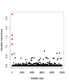
(b) $D=50,M=50\,000$

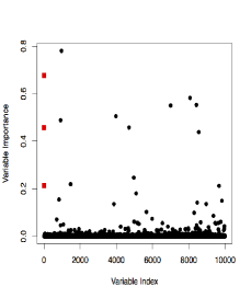
(c) $D=10,M=5\,000$

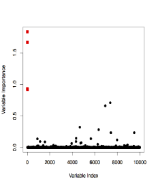
(d) $D=10,M=50\,000$

Figure 1: BART variable importance using sparse=TRUE and various number of trees $D$ and MCMC iterations $M$. Red squares (the first five covariates) are signals and black dots are noise variables.

5.1 Offline TVS

As a lead example in this section, we consider the benchmark Friedman data set (Friedman (1991)) with a vastly larger number of $p=10\,000$ predictors ${\boldsymbol{x}}_{i}\in[0,1]^{p}$ obtained by iid sampling from $\texttt{Uniform}(0,1)$ and responses ${\boldsymbol{Y}}=(Y_{1},\cdots Y_{n})^{\prime}$ obtained from (1) with $\sigma^{2}=1$ and

$$f_{0}({\boldsymbol{x}}_{i})=10\sin(\pi x_{i1}x_{i2})+20(x_{i3}-0.5)^{2}+10x_{i4}+5x_{i5}\quad\text{for $i=1,\dots,300$}.$$

Due to the considerable number of covariates, feeding all $10\,000$ predictors into a black box to obtain variable importance may not be computationally feasible and/or reliable. However, TVS can overcome this limitation by deploying subsets of predictors. For instance, we considered variable importance using the BART method (using the option sparse=TRUE for variable selection) with $D\in\{10,50\}$ trees and $M\in\{5\,000,50\,000\}$ MCMC iterations are plotted them in Figure 1. While increasing the number of iterations certainly helps in separating signal from noise, it is not necessarily obvious where to set the cutoff for selection. One natural rule would be selecting those variables which have been used at least once on average over the $M$ iterations. With $D=50$ and $M=50\,000$, this rule would identify $4$ true signals, leaving out the quadratic signal variable $x_{3}$. The computation took around $8.5$ minutes.

The premise of TVS is that one can deploy a weaker learner (such as a forest with fewer trees) which generates a random reward that roughly captures signal and is allowed to make mistakes. With reinforcement learning, one hopes that each round will be wrong in a different way so that mistakes will not be propagated over time. The expectation is that (a) feeding only a small subset $\mathcal{S}_{t}$ in a black box and (b) reinforcing positive outcomes, one obtains a more principled way of selecting variables and speeds up the computation. We illustrate the effectiveness of this mechanism below.

We use the offline local binary reward defined in (9). We start with a non-informative prior $a_{i}(0)=b_{i}(0)=1$ for $1\leq i\leq p$ and choose $T=10$ trees in BART so that variables are discouraged from entering the model too wildly. This is a weak learner which does not seem to do perfectly well for variable selection even after very many MCMC iterations (see Figure 1(d)). We use the TVS implementation in Table 1 with a dramatically smaller number $M\in\{100,500,1\,000\}$ of MCMC burn-in iterations for BART inside TVS. We will see below that large $M$ is not needed for TVS to unravel signal even with as few as $10$ trees.

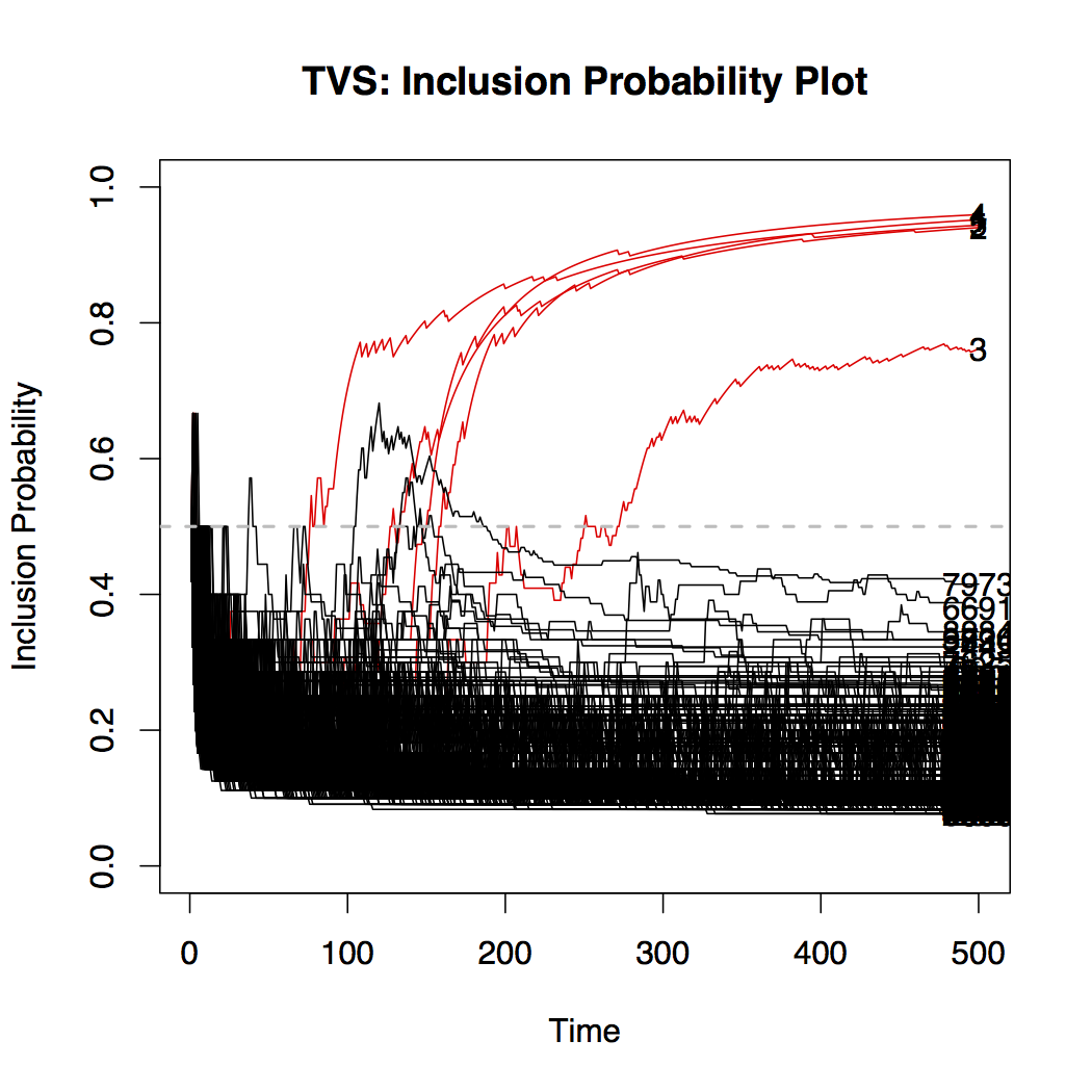
(a) $M=100$

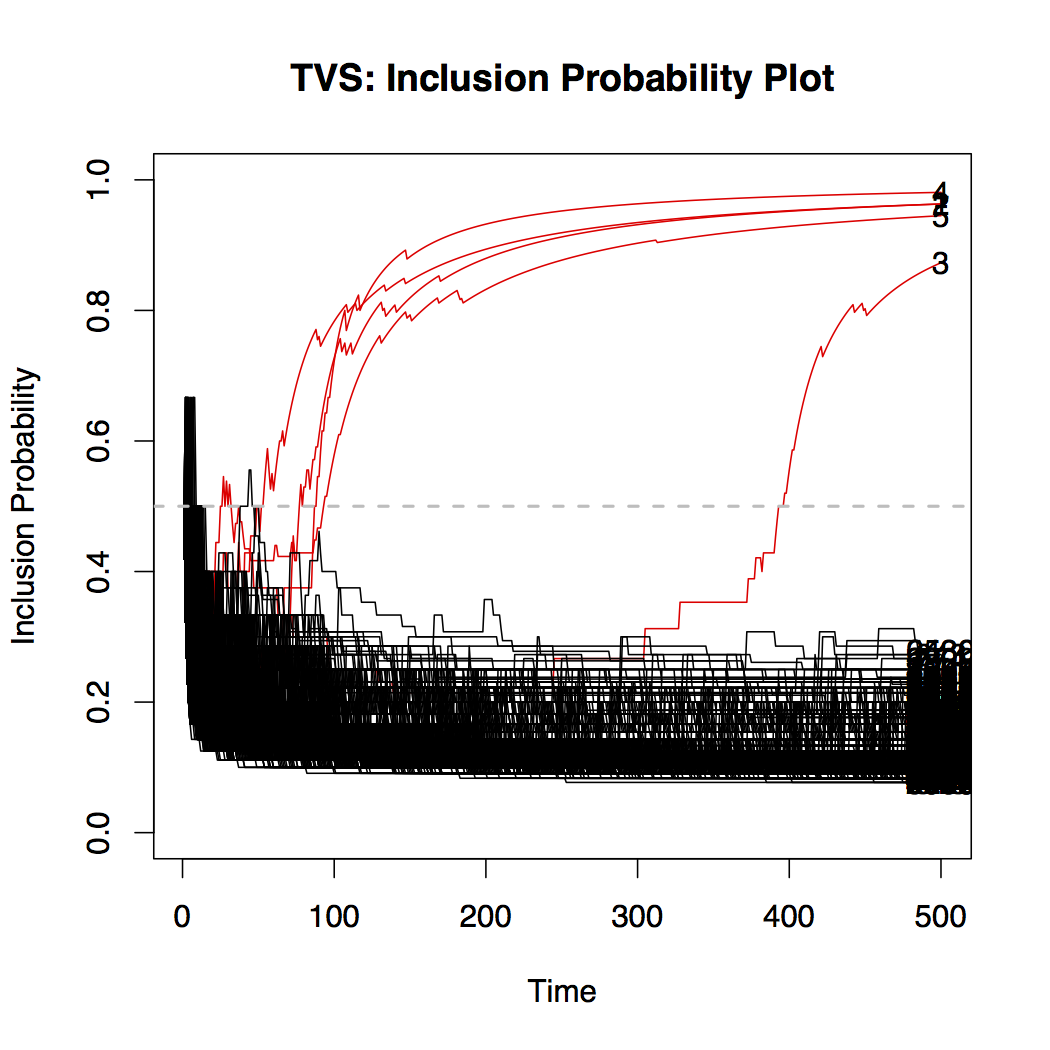
(b) $M=500$

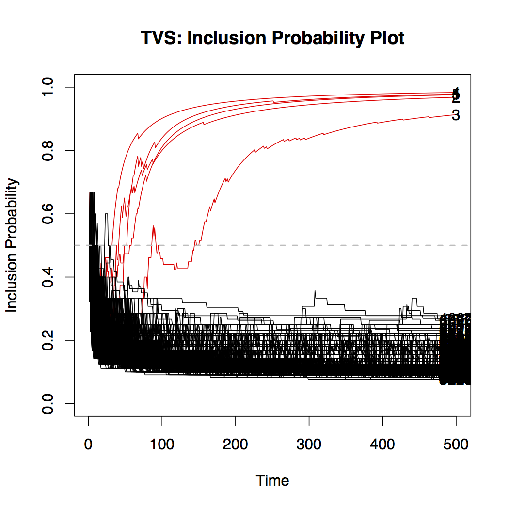
(c) $M=1\,000$

Figure 2: The evolution of inclusion probabilities (11) over “time” $t$ for the Friedman data set. The plot depicts posterior inclusion probabilities $\pi_{i}(t)$ in (11) over time (number of TVS iterations). Red lines indicate the $5$ signal variables and black lines indicate the noise variables.

TVS results are summarized in Figure 2, which depicts ‘posterior inclusion probabilities’ $\pi_{i}(t)$ defined in (11) over time $t$ (the number of plays), one line for each of the $p=10\,000$ variables. To better appreciate informativeness of $\pi_{i}(t)$’s, true variables $x_{1},\dots,x_{5}$ are depicted in red while the noise variables are black. Figure 2 shows a very successful demonstration for several reasons. The first panel (Figure 2(a)) shows a very weak learner (as was seen from Figure 1) obtained by sampling rewards only after $M=100$ burnin iterations. Despite the fact that learning at each step is weak, it took only around $T=300$ iterations (obtained in less than $40$ seconds!) for the $\pi_{i}(t)$ trajectories of the $5$ signals to cross the $0.5$ decision boundary. After $T=300$ iterations, the noise covariates are safely suppressed below the decision boundary and the trajectories $\pi_{i}(t)$ stabilize towards the end of the plot. Using more MCMC iterations $M$, fewer TVS iterations are needed to obtain a cleaner separation between signal and noise (noise $\pi_{t}$’s are closer to zero while signal $\pi_{t}$’s are closer to one). With enough internal MCMC iterations ($M=1\,000$ in the right panel), TVS is able to effectively separate signal from noise in around $200$ iterations (obtained in less than $2$ minutes). We have not seen such conclusive separation with plain BART (Figure 1) even after very many MCMC iterations which took considerably longer. Note that each iteration of TVS uses only a small subset of predictors and much fewer iterations $M$ and TVS is thereby destined to be faster than BART on the entire dataset (compare $8.5$ minutes for $20\,000$ iterations with $40$ seconds in Figure 2(a)). Applying the more traditional variable selection techniques was also not as successful. For example, the Spike-and-Slab LASSO (SSL) method ($\lambda_{1}=0.1$ and $\lambda_{0}\in\{0.1+k\times 10:k=1,\dots,10\}$) which relies on a linear model missed the quadratic predictor but identified all $4$ remaining signals with no false positives.

5.2 Online TVS

As the second TVS example, we focus on the case with many more observations than covariates, i.e. $n>>p$. As we already pointed out in Section 3.2, we assume that the dataset $\mathcal{D}_{n}=\{(Y_{i},\boldsymbol{x}_{i}):1\leq i\leq n\}$ has been partitioned into mini-batches $\mathcal{D}_{t}$ of size $s=n/T$. We deploy our online TVS method (Table 1 with C2^⋆) to sequentially screen each batch and transmit the posterior information onto the next mini-batch through a prior. This should be distinguished from streaming variable selection, where new features arrive at different time points (Foster and Stine (2008)). Using the notation $r_{t}\equiv r(\mathcal{S}_{t},\mathcal{D}_{t})$ in (8) with $\mathcal{D}_{t}=\{(Y_{i},\boldsymbol{x}_{i}):(t-1)s+1\leq i\leq ts\}$ and having processed $t-1$ mini-batches, one can treat the beta posterior as a new prior for the incoming data points, where

$$\pi(\boldsymbol{\theta}\,|\,r_{1},\dots,r_{t})\propto\pi(\boldsymbol{\theta}\,|\,r_{1},\dots,r_{t-1})\prod_{i\in\mathcal{S}_{t}}\theta_{i}^{\gamma_{i}^{t}}(1-\theta_{i})^{1-\gamma_{i}^{t}}.$$

Parsing the observations in batches will be particularly beneficial when processing the entire dataset (with overwhelmingly many rows) is not feasible for the learning algorithm. TVS leverages the fact that applying a machine learning method $T$ times using only a subset of $s$ observations and a subset $\mathcal{S}_{t}$ of variables is a lot faster than processing the entire data. While the posterior distribution of $\theta_{i}$’s after one pass through the entire dataset will have seen all the data $\mathcal{D}_{n}$, $\theta_{i}$’s can be interpreted as the frequentist probability that the screening rule picks a variable $x_{i}$ having access to only $s$ measurements.

We illustrate this sequential learning method on a challenging simulated example from (Liang et al., 2018, Section 5.1) . We assume that the explanatory variables ${\bf x}_{i}\in[0,1]^{p}$ have been obtained from $x_{ij}=(e_{i}+z_{ij})/2$ for $1\leq i\leq n$ and $1\leq j\leq p$, where $e,z_{ij}\stackrel{{\scriptstyle iid}}{{\sim}}\mathcal{N}(0,1)$. This creates a sample correlation of about $0.5$ between all variables. The responses ${\bf Y}=(Y_{1},\cdots,Y_{n})^{\prime}$ are then obtained from (1), where

$$f_{0}({\bf x}_{i})=\frac{10x_{i2}}{1+x_{i1}^{2}}+5\sin(x_{i3}x_{i4})+2x_{i5}$$

with $\sigma^{2}=0.5$. This is a challenging scenario due to (a) the non-negligible correlation between signal and noise, and (b) the non-linear contributions of $x_{1}-x_{4}$. Unlike Liang et al. (2008) who set $n=p=500$, we make the problem considerably more difficult by choosing $n=20\,000$ and $p=1\,000$. We would expect a linear model selection method to miss these two nonlinear signals. Indeed, the Spike-and-Slab LASSO method (using $\lambda_{1}=0.1$ and $\lambda_{0}\in\{0.1+k\times 10:k=1,\dots,10\}$ only identifies variables $x_{1},x_{2}$ and $x_{5}$. Next, we deploy the BART method with variable selection (Linero 2016) by setting sparse=TRUE (Linero and Yang (2018)) and $50$ trees in the BART software (Chipman et al. (2010)). The choice of $50$ trees for variable selection was recommended in Bleich et al. (2014) and was seen to work very well. Due to the large size of the dataset, it might be reasonable to first inquire about variable selection from smaller fractions of data. We consider random subsets of different sizes $s\in\{100,500,1\,000\}$ as well as the entire dataset and we run BART for $M=20\,000$ iterations. Figure 3 depicts BART importance measures (average number of times each variable was used in the forest). We have seen BART separating the signal from noise rather well on batches of size $s\geq 1\,000$ and with MCMC iterations $M\geq 10\,000$. The scale of the importance measure depends on $s$ and it is not necessarily obvious where to make the cut for selection. A natural (but perhaps ad hoc) criterion would be to pick variables which were on average used at least once. This would produce false negatives for smaller $s$ and many false positives ($29$ in this example) for $s=20\,000$. The Hamming distance between the true and estimated model as well as the computing times are reported in Table 1. This illustrates how selection based on the importance measure is difficult to automate. While visually inspecting the importance measure for $M=20\,000$ and $s=20\,000$ (the entire dataset) in Figure 3(d) is very instructive for selection, it took more than $70$ minutes on this dataset. To enhance the scalability, we deploy our reinforcement learning TVS method for streaming batches of data.

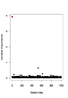
(a) $s=100$

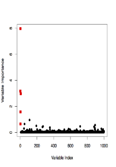
(b) $s=500$

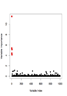
(c) $s=1\,000$

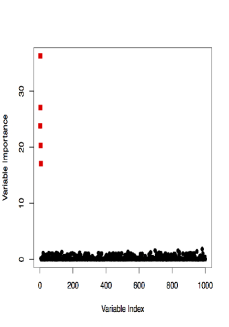
(d) Entire Data

Figure 3: BART variable importance using $T=20\,000$ (using $50$ trees and sparse=TRUE) and various data subsets. Red squares (the first five covariates) are signals and black dots are noise variables.

	$s=100$		$s=200$		$s=500$		$s=1\,000$		$s=5\,000$		$s=10\,000$		$s=20\,000$
T	Time	HAM	Time	HAM	Time	HAM	Time	HAM	Time	HAM	Time	HAM	Time	HAM
$5\,000$	6.7	4	7.7	5	11.4	3	21.5	2	103.1	3	264.2	8	794.1	16
$10\,000$	16.2	4	16	4	23.6	2	37.8	3	213	8	549.9	18	2368.4	25
$20\,000$	27.3	4	31.1	4	47.7	1	74.7	1	418.4	10	1090.6	21	4207.4	29

Table 1: Computing times (in seconds) and Hamming distance of BART on subsets of observations using all $p$ covariates. Hamming distance compares the true model with a model obtained by truncating the BART importance measure at 1.

Using the online local reward (10) with BART (with $10$ trees and sparse=TRUE and $M$ iterations) on batches of data $\mathcal{D}_{n}$ of size $s$. This is a weaker learning rule than the one considered in Figure 3 ($50$ trees). Choosing $s=100$ and $M=10\,000$, BART may not be able to obtain perfect signal isolation on a single data batch (see Figure 3(a) which identifies only one signal variable). However, by propagating information from one batch onto the next, TVS is able to tease out more signal (Figure 4(a)). Comparing Figure 3(b)) and Figure 4(c) is even more interesting, where TVS inclusion probabilities for all signals eventually cross the decision boundary after merely $40$ TVS iterations. There is ultimately a tradeoff between the batch size $s$ and the number of iterations needed for the TVS to stabilize. For example, with $s=1\,000$ one obtains a far stronger learner (Figure 3(c)), but the separation may not be as clear after only $T=n/s=20$ TVS iterations (Figure 4(d)). One can increase the number of TVS iterations by performing multiple passes through the data after bootstrapping the entire dataset and chopping it into new batches which are a proxy for future data streams. Plots of TVS inclusion probabilities after $5$ such passes through the data are in Figure 5. Curiously, one obtains much better separation even for $s=200$ and with larger batches ($s=500$) the signal is perfectly separated. Note that TVS is a random algorithm and thereby the trajectories in Figure 5 at the beginning are slightly different from Figure 4. Despite the random nature, however, we have seen the separation apparent from Figure 5 occur consistently across multiple runs of the method.

Several observations can be made from the timing and performance comparisons presented in Table 2. When the batch size is not large enough, repeated runs will not help. The Hamming distance in all cases only consists of false negatives and can be decreased by increasing the batch size or increasing the number of iterations and rounds. Computationally, it seems beneficial to increase the batch size $s$ and supply enough MCMC iterations. Variable selection accuracy can also be increased with multiple rounds.

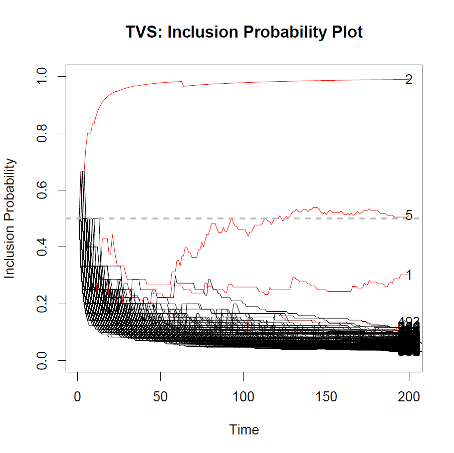
(a) $s=100$

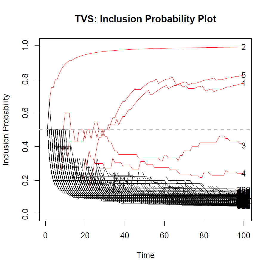
(b) $s=200$

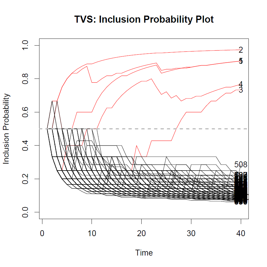
(c) $s=500$

(d) $s=1\,000$

Figure 4: TVS inclusion probabilities $T=10\,000$ (using $10$ trees and sparse=TRUE) and various batch sizes after single pass through the data.

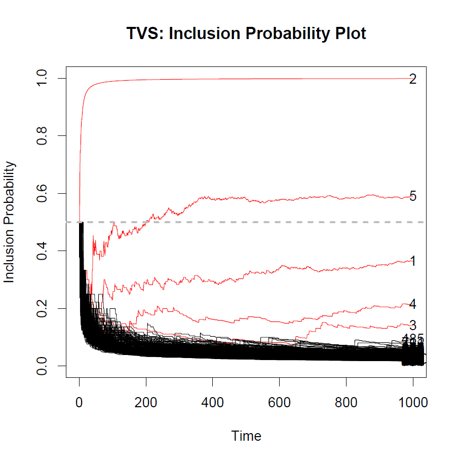
(a) $s=100$

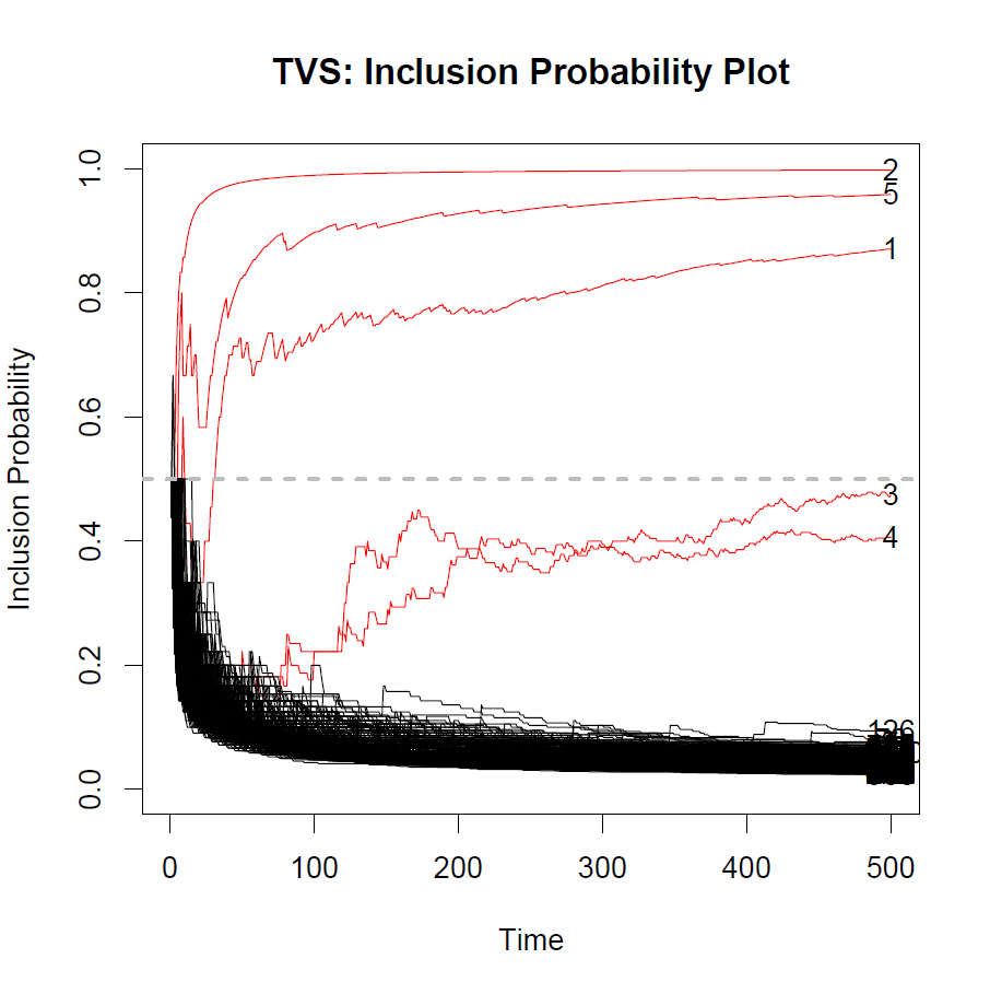
(b) $s=200$

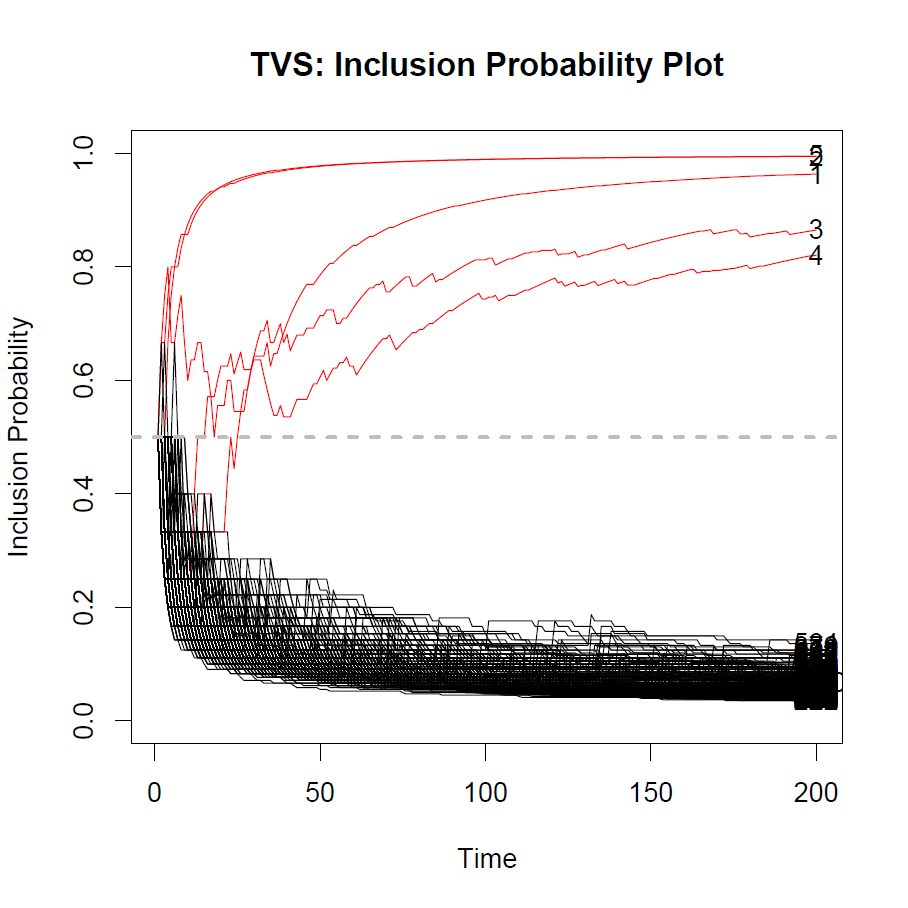
(c) $s=500$

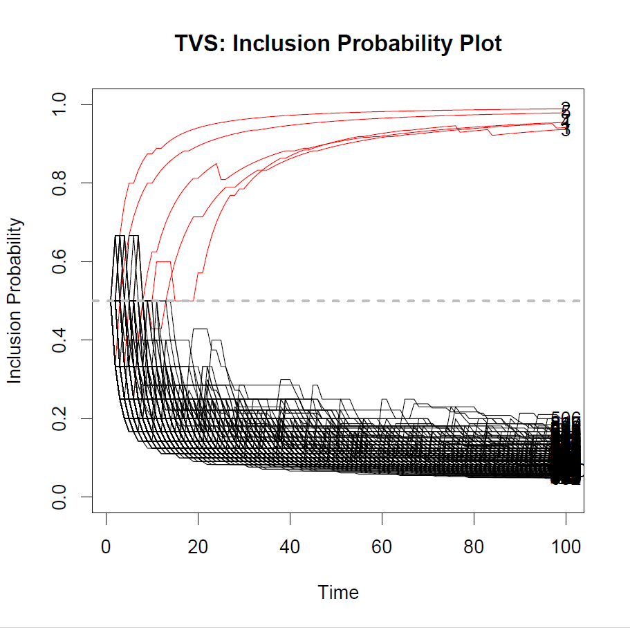
(d) $s=1\,000$

Figure 5: TVS inclusion probabilities $T=10\,000$ (using $10$ trees and sparse=TRUE) and various batch sizes after $5$ passes through the data.

	$s=100$		$s=200$		$s=500$		$s=1\,000$
	Time	HAM	Time	HAM	Time	HAM	Time	HAM
$T=500$
$1$ round	58.9	4	34.1	3	19.3	3	15.7	4
$5$ rounds	251.5	4	165	3	91.2	3	68.7	2
$10$ rounds	467.5	4	348.8	3	187.8	3	137.2	1
$T=1\,000$
$1$ round	84	4	49.8	3	29.5	3	23.6	2
$5$ rounds	411.8	4	241.5	3	140.8	1	111.4	0
$10$ rounds	870.6	3	507	2	288.2	1	224.2	0
$T=1\,0000$
$1$ round	541.8	3	330.9	2	220.4	0	182.8	0
$5$ rounds	2421.2	3	1501.9	2	1060.2	0	972.2	0
$10$ rounds	4841.9	3	3027.9	0	2248.3	0	2087.6	0

Table 2: Computing times (in seconds) and Hamming distance for TVS using different batch sizes $s$ and BART iterations $T$ and multiple passes through the data. The Hamming distance compares the true model with a model truncating the last TVS inclusion probability at 0.5.

6 Simulation Study

We further evaluate the performance of TVS in a more comprehensive simulation study. We compare TVS with several related non-parametric variable selection methods and with classical parametric ones. We assess these methods based on the following performance criteria: False Discovery Proportion (FDP) (i.e. the proportion of discoveries that are false), Power (i.e. the proportion of true signals discovered as such), Hamming Distance (between the true and estimated model) and Time.

6.1 Offline Cases

For a more comprehensive performance evaluation, we consider the following $4$ mean functions $f_{0}(\cdot)$ to generate outcomes using (1). For each setup, we summarize results over $50$ datasets of a dimensionality $p\in\{1\,000,10\,000\}$ and a sample size $n=300$.

• Linear Setup: The regressors ${\boldsymbol{x}}_{i}$ are drawn independently from $N(0,\Sigma)$, where $\Sigma=(\sigma_{jk})_{j,k=1,1}^{p,p}$ with $\sigma_{jj}=1$ and $\sigma_{jk}=0.9^{|j-k|}$ for $j\neq k$. Only the first $5$ variables are related to the outcome (which is generated from (1) with $\sigma^{2}=5$) via the mean function $f_{0}(\boldsymbol{x}_{i})=x_{i1}+2x_{i2}+3x_{i3}-2x_{i4}-x_{i5}$.

• Friedman Setup: The Friedman setup was described earlier in Section 1. In addition, we now introduce correlations of roughly $0.3$ between the explanatory variables.

• Forest Setup: We generate ${\boldsymbol{x}_{i}}$ from $N(0,\Sigma)$, where $\Sigma=(\sigma_{jk})_{j,k=(11)}^{p,p}$ with $\sigma_{jj}=1$ and $\sigma_{jk}=0.3^{|j-k|}$ for $j\neq k$. We then draw the mean function $f_{0}(\cdot)$ from a BART prior with $200$ trees, using only first $5$ covariates for splits. The outcome is generated from (1) with $\sigma^{2}=0.5$.

• Liang et al (2016) Setup: This setup was described earlier in Section 5.2. We now use $\sigma^{2}=0.5$.

We run TVS with $M=500$ and $M=1\,000$ internal BART MCMC iterations and with $T=500$ TVS iterations. As two benchmarks for comparison, we consider the original BART method (in the R-package BART) and a newer variant called DART (Linero and Yang (2018)) which is tailored to high-dimensional data and which can be obtained in BART by setting sparse=TRUE ( a=1, b=1). We ran BART and DART for $M=50\,000$ MCMC iterations using the default prior settings with $D=20$, $D=50$ and $D=200$ trees for BART and $D=10$, $D=50$ and $D=200$ trees for DART. We considered two variable selection criteria: (1) posterior inclusion probability (calculated as the proportion of sampled forests that split on a given variable) at least $0.5$ (see Linero (2018) and Bleich et al. (2014) for more discussion on variable selection using BART), (2) the average number of splits in the forest (where the average is taken over the $M$ iterations) at least $1$. We report the settings with the best performance, i.e. BART with $D=20$ trees and DART with $D=50$ trees using the second inclusion criterion. The third benchmark method we use for comparisons is the Spike-and-Slab LASSO (Rockova and George (2018)) implemented in the R-package SSLASSO with lambda1=0.1 and the spike penalty ranging from $\lambda_{1}$ to the number of variables $p$ (i.e. lambda0 = seq(1, p, length=p)). We choose the same set of variable chosen by SSLASSO function after the regularization path has stabilized using the model output. We have also implemented Sure Independence Screen (SIS) (Fan and Lv (2008)) as a variable filter before applying BART variable selection. Next, we applied one of the benchmark Bayesian variable selection methods, the horseshoe prior (van der Pas et al. (2017); Carvalho et al. (2010)) implementation from the R-package horseshoe. We run the Markov chain for $55\,000$ iterations, discarding the first $5\,000$ as a burnin period. Variable selection is performed by checking whether $0$ is contained in the credible set (see van der Pas et al. (2019)). Finally, we implement the LASSO (Tibshirani (2011)) and report the model chosen according to the $1$-s.e. rule (Friedman et al. (2001))).

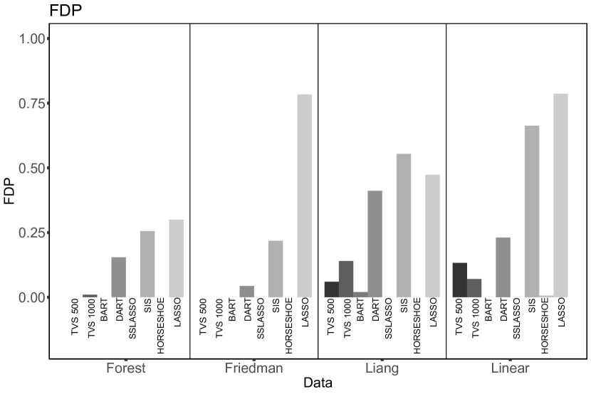
(a) FDP

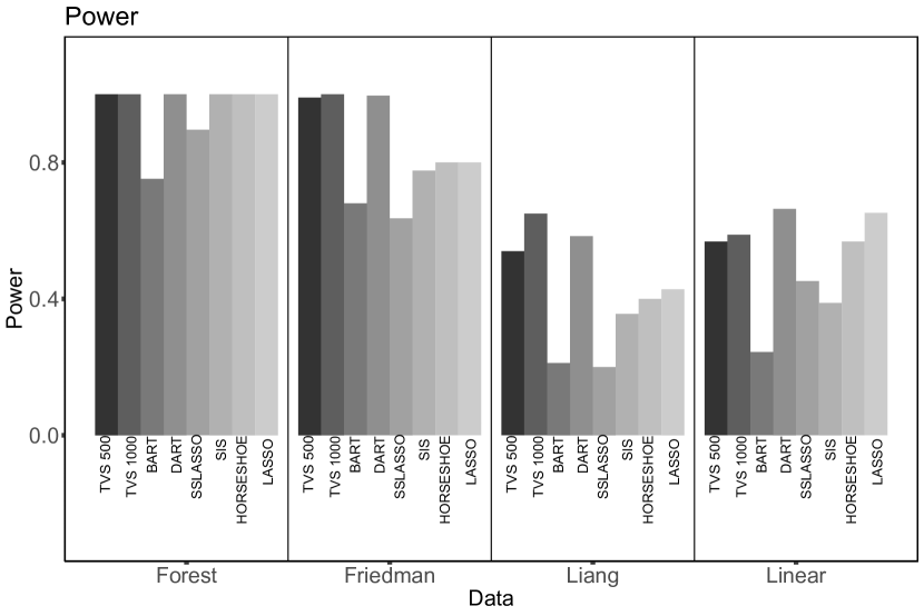
(b) Power

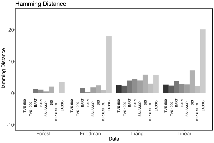
(c) Hamming Distance

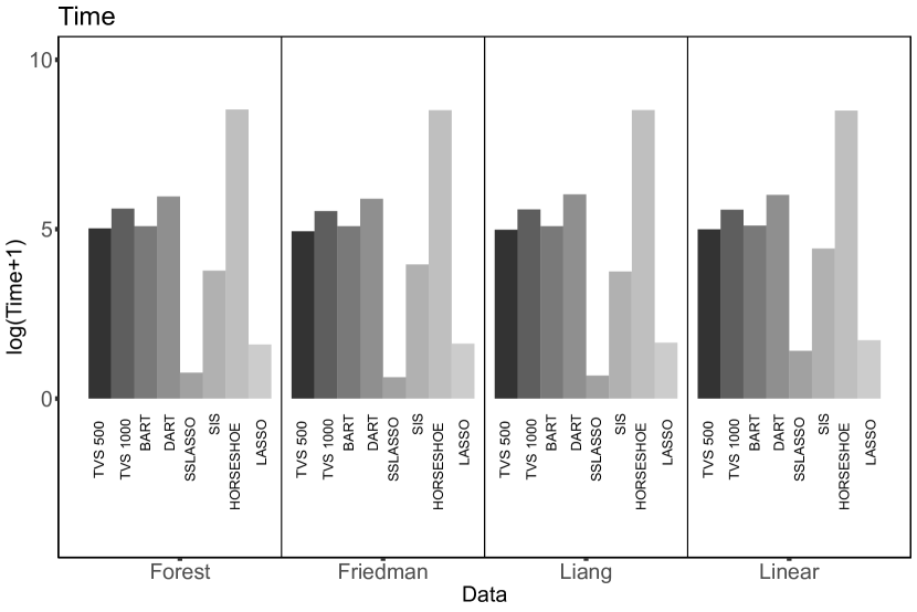
(d) Time

Figure 6: Graphs denoting FDP (6(a)), Power (6(b)), Hamming Distance (6(c)), and Time (6(d)) for the $4$ choices of $f_{0}$ assuming $p=10\,000$ and $n=300$. The $x$-axis denotes the choice of $f_{0}$ and the various methods are marked with various shades of gray. For TVS, we have two choices $M=500$ and $M=1\,000$.

We report the average performance (over $50$ datasets) for $p=10\,000$ in Figure 6 and the rest (for $p=1\,000$) in the Appendix. Recall that the model estimated by TVS is obtained by truncating $\pi_{i}(500)$’s at $0.5$. In terms of the Hamming distance, we notice that TVS performs best across-the-board. DART (with $D=50$) performs consistently well in terms of variable selection, but the timing comparisons are less encouraging. BART (with $D=20$) takes a relatively comparable amount of time as TVS with $M=1\,000$, but suffers from less power. SS-LASSO’s performance is strong, in particular for the less non-linear data setups. The performance of TVS is seen to improve with $M$. SIS is a screening method based on a linear model assumption. Albeit faster than TVS, we observe that SIS generally over-selects. In addition, SIS screens out key signals with non-linear effects (Liang and Friedman datasets). The Horseshoe prior performs very well but is much slower. LASSO seems to overfit, in spite of the 1-se rule.

We also implement a stopping criterion for TVS based on the stabilization of the inclusion probabilities $\pi_{i}(t)=\frac{a_{i}(t)}{a_{i}(t)+b_{i}(t)}$. One possibility is to stop TVS when the estimated model $\smash{\widehat{\mathcal{S}}}_{t}$ obtained by truncating $\pi_{i}(t)$’s at $0.5$ has not changed for over, say, $100$ consecutive TVS iterations. With this convergence criterion, the convergence times differs across the different data set-ups. Generally, TVS is able to converge in $\sim 200$ iterations for $p=1\,000$ and $\sim 300$ iterations for $p=10\,000$. While the computing times are faster, TVS may be more conservative (lower FDP but also lower Power). The Hamming distance is hence a bit larger, but comparable to TVS with $500$ iterations (Appendix C.1)

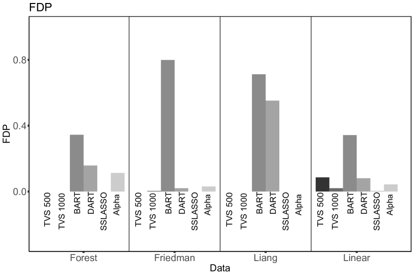
(a) FDP

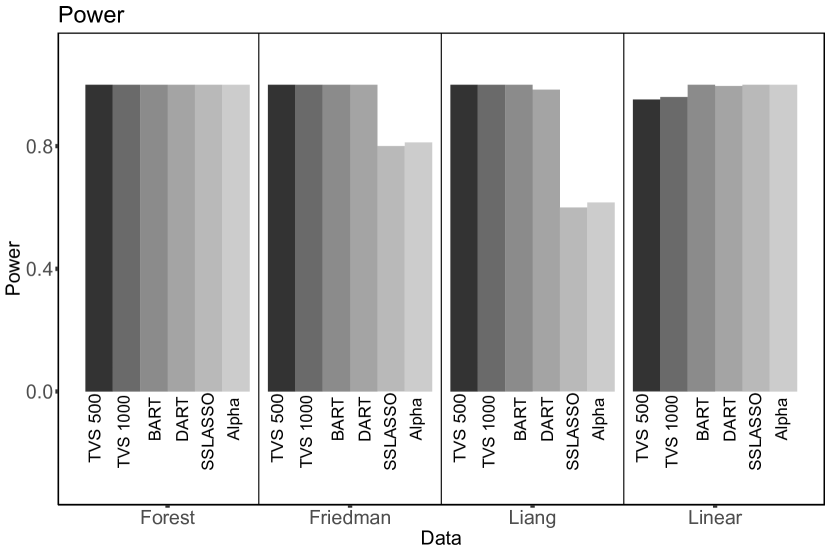
(b) Power

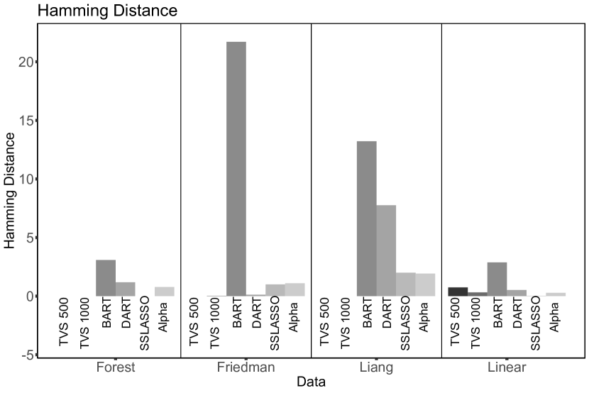
(c) Hamming Distance

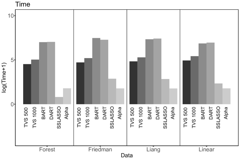
(d) Time

Figure 7: Graphs denoting FDP (7(a)), Power (7(b)), Hamming Distance (7(c)), and Time (7(d)) for the $4$ choices of $f_{0}$ assuming $p=1\,000$ and $n=10\,000$. The $x$-axis denotes the choice of $f_{0}$ and the various methods are marked with various shades of gray. For TVS, we have two choices $M=500$ and $M=1\,000$, both with $s=1000$.

6.2 Online Cases

We now consider a simulation scenario where $n>>p$, i.e. $p=1\,000$ and $n=10\,000$. As described earlier in Section 5.2, we partition the data into minibatches $(\boldsymbol{Y}^{(b)},\boldsymbol{X}^{(b)})$ of size $s$, where $\boldsymbol{Y}^{(b)}=(Y_{i}:(b-1)s+1\leq i\leq bs)$ and $\boldsymbol{X}^{(b)}=[\boldsymbol{x}_{i}:(b-1)s+1\leq i\leq bs]^{\prime}$ for $b=1,\dots,n/s$ with $s\in\{500,1000\}$ and $M\in\{500,1000\}$ using $D=10$ trees. In this study, we consider the same four set-ups as in Section 6.1. We implemented TVS with a fixed number of rounds $r\in\{1,5,10\}$ and a version with a stopping criterion based on the stabilization of the inclusion probabilities $\pi_{i}(t)=\frac{a_{i}(t)}{a_{i}(t)+b_{i}(t)}$. This means that TVS will terminate when the estimated model $\widehat{\mathcal{S}}_{t}$ obtained by truncating $\pi(t)$’s at $0.5$ has not changed for $100$ consecutive iterations. The results using the stopping criterion are reported in Figure 7 and the rest is in the Appendix (Section LABEL:sec:appendix_online_simul ). As before, we report the best configuration for BART and DART, namely $D=20$ for BART and $D=50$ for DART (both with $50\,000$ MCMC iterations). For both methods, there are non-negligible false discoveries and the timing comparisons are not encouraging. In addition, we could not apply both BART and DART with $n\geq 50\,000$ observations due to insufficient memory. For TVS, we found the batch size $s=1\,000$ to work better, as well as running the algorithm for enough rounds until the inclusion probabilities have stabilized (Figure 7 reports the results with a stopping criterion). The results are very encouraging.

Streaming feature selection methods are still being developed (Wang et al. (2018); Fahy and Yang ; Ramdas et al. ; Javanmard et al. (2018)). We have compared our online variant with the $\alpha$-investing method for streaming variable selection of Zhou et al. (2006). This method dynamically adjusts $p$-value thresholds for adding features to the model. We run this method using $p$-values from applying linear regression on batches of streaming data. The results are shown in Figure 7. This procedure performs well in Forest and Linear set-ups but misses the key non-linear variables in Friedman and Liang setups. While SSLASSO’s performance is very strong, we notice that in the non-linear setup of Liang et al. (2018) there are false non-discoveries.

7 Application on Real Data

7.1 HIV Data

We will apply (offline) TVS on a benchmark Human Immunodeficiency Virus Type I (HIV-I) data described and analyzed in Rhee et al. (2006) and Barber et al. (2015). This publicly available dataset consists of genotype and resistance measurements (decrease in susceptibility on a log scale) to three drug classes: (1) protease inhibitors (PIs), (2) nucleoside reverse transcriptase inhibitors (NRTIs), and (3) non-nucleoside reverse transcriptase inhibitors (NNRTIs).

The goal in this analysis is to find mutations in the HIV-1 protease or reverse transcriptase that are associated with drug resistance. Similarly as in Barber et al. (2015) we analyze each drug separately. The response $Y_{i}$ is given by the log-fold increase of lab-tested drug resistance in the $i^{th}$ sample with the design matrix $X$ consisting of binary indicators $x_{ij}\in\{0,1\}$ for whether or not the $j^{th}$ mutation has occurred at the $i^{th}$ sample.

In an independent experimental study, (Rhee et al., 2005) identified mutations that are present at a significantly higher frequency in virus samples from patients who have been treated with each class of drugs as compared to patients who never received such treatments. While, as with any other real data experiment, the ground truth is unknown, we treat this independent study are a good approximation to the ground truth. Similarly as Barber et al. (2015), we only compare mutation positions since multiple mutations in the same position are often associated with the same drug resistance outcomes.

For illustration, we now focus on one particular drug called Lopinavir (LPV). There are $p=206$ mutations and $n=824$ independent samples available for this drug. TVS was applied to this data for $T=500$ iterations with $M=1\,000$ inner BART iterations. In Figure 8, we differentiate those mutations whose position were identified by Rhee et al. (2005) and mutations which were not identified with blue and red colors, respectively. From the plot of inclusion probabilities in Figure 8(a), it is comforting to see that only one unidentified mutation has a posterior probability $\pi_{j}(t)$ stabilized above the $0.5$ threshold. Generally, we observe the experimentally identified mutations (blue curves) to have higher inclusion probabilities.

(a) TVS Inclusion Probabilities

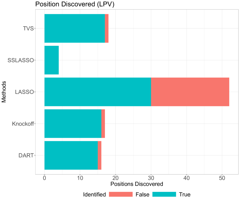
(b) Comparisons with other Methods

Figure 8: Thompson Variable Selection on the LPV dataset. (Left) Trajectories of the inclusion probabilities $\pi_{j}(t)$. (Right) Number of signals discovered, where blue denotes the experimentally validated signals and red are the unvalidated ones.

Comparisons are made with DART, Knockoffs (Barber et al., 2015), LASSO (10-fold cross-validation), and Spike-and-Slab LASSO (Rockova and George (2018)), choosing $\lambda_{1}=0.1$ and $\lambda_{0}\in\{\lambda_{1}+10\times k\mathchar 24635\relax\;k=0,1,\dots,p\}$). Knockoffs, LASSO, and the Spike-and-Slab LASSO assume a linear model with no interactions. DART was implemented using $T=50$ trees and $50\,000$ MCMC iterations, where we select those variables whose average number splits was at least one. The numbers of discovered Positions for each method are plotted in Figure 8(b). While LASSO selects many more experimentally validated mutations, it also includes many unvalidated ones. TVS, on the other hand, has a very small number of “false discoveries” while maintaining good power. Additional results are included in the Appendix (Section LABEL:sec:supplement_hiv).

7.2 Durable Goods Marketing Data Set

Our second application examines a cross-sectional dataset described in Ni et al. (2012) consisting of durable goods sales data from a major anonymous U.S. consumer electronics retailer. The dataset features the results of a direct-mail promotion campaign in November 2003 where roughly half of the $n=176\,961$ households received a promotional mailer with $10\$$ off their purchase during the promotion time period (December 4-15). If they did purchase, they would get $10\%$ off on a subsequent purchase through December. The treatment assignment was random. The data contains $p=146$ descriptors of all customers including prior purchase history, purchase of warranties etc. We will investigate the effect of the promotional campaign (as well as other covariates) on December sales. In addition, we will interact the promotion mail indicator with customer characteristics to identify the “mail-deal-prone” customers.

We dichotomized December purchase (in dollars) to create a binary outcome $Y_{i}=\mathbb{I}(\texttt{December-sales}_{i}>0)$ for whether or not the $i^{th}$ customer made any purchase in December. Regarding predictor variables, we removed any variables with missing values and any binary variables with less than $10$ samples in one group. This pre-filtering leaves us with $114$ variables whose names and descriptive statistics are reported in Section LABEL:sec:additional_marketing_data in the Appendix. We interact the promotion mail indicator with these variables to obtain $p=227$ predictors. Due to the large volume of data ($n\approx 180\,000$), we were unable to run DART and BART (BART package implementation) due to memory problems. This highlights the need for TVS as a variable selector which can handle such voluminous data.

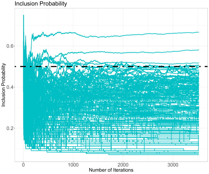
(a) $s=1\,000$

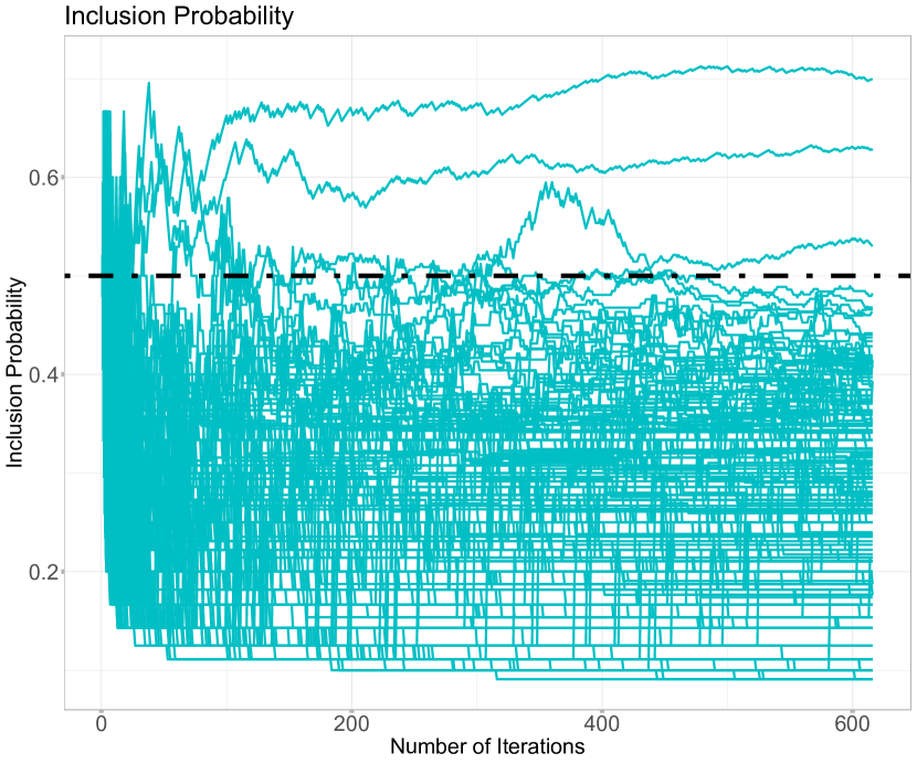
(b) $s=2\,000$

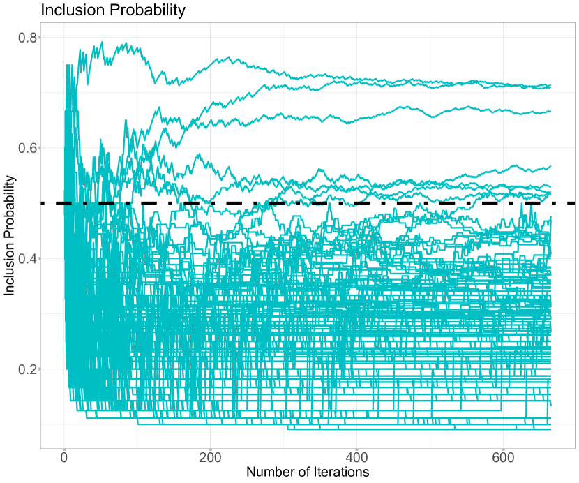
(c) $s=5\,000$

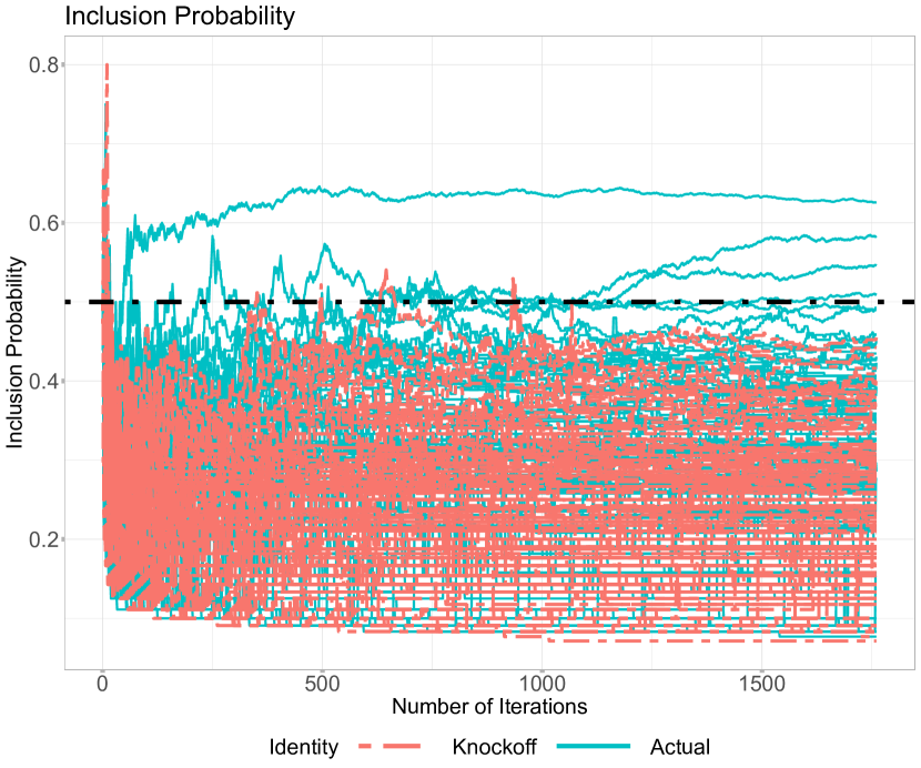
(d) $s=1\,000$

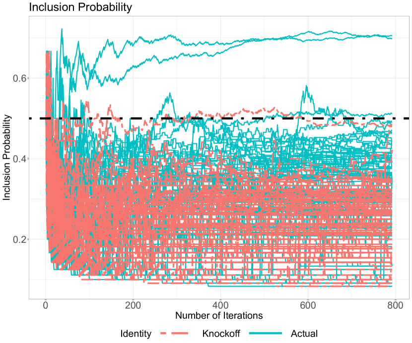
(e) $s=2\,000$

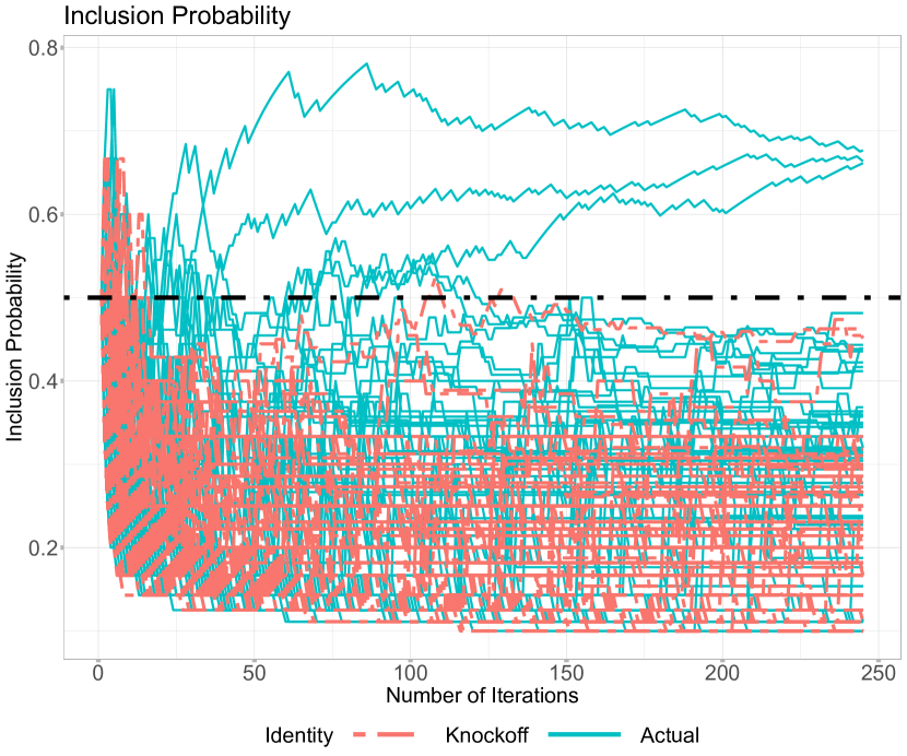
(f) $s=5\,000$

Figure 9: Thompson Variable Selection on the marketing data. (Left) Trajectories of the inclusion probabilities $\pi_{j}(t)$ without knockoffs. (Right) Trajectories of the inclusion probabilities $\pi_{j}(t)$ with knockoffs (in red).

Unlike the HIV-I data in Section 7.1, there is no proxy for the ground truth. To understand the performance quality of TVS, we added $227$ normally distributed knockoffs. The knockoffs are generated using create.second_order function in the knockoff R package (Patterson and Sesia (2018)) using a Gaussian Distributions with the same mean and covariance structure (Candes et al. (2018)). We run TVS with a batch size $s\in\{1\,000,2\,000,5\,000\}$ and $M=1\,000$ inner iterations until the posterior probabilities have stabilized. The inclusion probabilities are plotted in Figure 9 for two cases (a) without knockoffs (the first row) and (b) with knockoffs (the second row). It is interesting to note that, apart from one setting with $s=1\,000$, the knockoff trajectories are safely suppressed below $0.5$ (dashed line). Both with and without knockoffs, TVS chooses ‘the number of months with purchases in past 24 month’ and ‘the November Promotion Sales’ as important variables. The selected variables for each combination of settings are summarized in Table 3.

	$s=1\,000$		$s=2\,000$		$s=5\,000$
Knockoff	Yes	No	Yes	No	Yes	No
total number of medium ticket items in previous 60 months	0.30	0.51	0.51	0.46	0.44	0.51
total number of small ticket items in previous 60 months	0.49	0.52	0.40	0.41	0.25	0.53
number of months shopped once in previous 12 months	0.34	0.41	0.44	0.42	0.41	0.57
number of months shopped once in previous 24 months	0.63	0.67	0.70	0.63	0.66	0.71
count of unique purchase trips in previous 24 months	0.55	0.26	0.48	0.53	0.68	0.67
total number of items purchased in previous 12 months	0.51	0.30	0.24	0.21	0.24	0.11
promo_nov period: total sales	0.58	0.58	0.71	0.70	0.33	0.45
mailed in holiday 2001 mailer	0.25	0.43	0.08	0.41	0.42	0.52
percent audio category sales of total sales $\times$ mail indicator	0.41	0.50	0.15	0.28	0.13	0.10
promo_nov period: total sales $\times$ mail indicator	0.15	0.35	0.46	0.41	0.66	0.71
indicator of holiday mailer 2002 promotion response $\times$ mail indicator	0.19	0.38	0.44	0.21	0.44	0.52

Table 3: Variables Selected by TVS with different $s$ and with/without knockoff. The numbers report conditional inclusion probabilities $\pi_{i}(t)$ after convergence, where values above $0.5$ are in bold.

Finally, we used the same set of variables (including knockoff variables) for different variable selection methods and recorded the number of knockoffs chosen by each one. We used BART ($D=20$, MCMC iteration = $50\,000$), and DART ($D=50$, MCMC iteration = $50\,000$) with the same selection criteria as before, i.e. a variable is selected if it was split on average at least once. We also consider LASSO where the sparsity penalty $\lambda$ was chosen by cross-validation. BART and DART cannot be run on the entire data set so we only run it on a random subset of $10\,000$ data points. While TVS with large enough $s$ does not include any of the knockoffs, LASSO does include $14$ and DART includes $4$.

8 Discussion

Our work pursues an intriguing connection between spike-and-slab variable selection and binary bandit problems. This pursuit has lead to a proposal of Thompson Variable Selection, a reinforcement learning wrapper algorithm for fast variable selection in high dimensional non-parametric problems. In related work, Liu et al. (2018) developed an ABC sampler for variable subsets through a split-sample approach by (a) first proposing a subset $\mathcal{S}_{t}$ from a prior, (b) keeping only those subsets that yield pseudo-data that are sufficiently close to the left-out sample. TVS can be broadly regarded as a reinforcement learning elaboration of this strategy where, instead of sampling from a (non-informative) prior $\pi(\mathcal{S}_{t})$, one “updates the prior $\pi(\mathcal{S}_{t})$” by learning from previous successes.

TVS can be regarded as a stochastic optimization approach to subset selection which balances exploration and exploitation. TVS is suitable in settings when very many predictors and/or very many observations can be too overwhelming for machine learning. By sequentially parsing subsets of data and reinforcing promising covariates, TVS can effectively separate signal from noise, providing a platform for interpretable machine learning. TVS minimizes regret by sequentially computing a median probability model rule obtained by truncating sampled mean rewards. We provide bounds for this regret without necessarily assuming that the mean arm rewards be unrelated. We observe strong empirical performance of TVS under various scenarios, both on real and simulated data. The TVS approach, coupled with BART, captures non-linearities and may thus be beneficial over linear techniques. In addition, TVS scales to very large datasets.

Thompson sampling is ultimately designed to minimize regret, not to select the best arms. Bubeck et al. (2009) point out that algorithms satisfying regret bounds of order $\log(T)$ can be far from optimal for finding the best arm. Russo (2016) proposed a ‘top-two’ sampling version of Thompson sampling which is tailored for single best-arm identification. Alternative algorithms have been proposed including the Successive Elimination algorithm of Even-Dar et al. (2006) for single top-arm identification and the SAR (Successive Accepts Rejects) algorithm of Bubeck et al. (2013) for top $m$-arm identification. These works suggest possible refinements of our approach for directly targeting multiple best arms in correlated combinatorial bandits.

References

- Agrawal and Goyal (2012) Agrawal, S. and N. Goyal (2012). Analysis of Thompson sampling for the multi-armed bandit problem. In Conference on Learning Theory.
- Barber et al. (2015) Barber, R. F., E. J. Candès, et al. (2015). Controlling the false discovery rate via knockoffs. The Annals of Statistics 43(5), 2055–2085.
- Barbieri et al. (2020) Barbieri, M., J. O. Berger, E. I. George, and V. Rockova (2020). The median probability model and correlated variables. Bayesian Analysis (to appear).
- Barbieri and Berger (2004) Barbieri, M. M. and J. O. Berger (2004). Optimal predictive model selection. Annals of Statistics 32(3), 870–897.
- Bhattacharya et al. (2016) Bhattacharya, A., A. Chakraborty, and B. K. Mallick (2016). Fast sampling with Gaussian scale mixture priors in high-dimensional regression. Biometrika 103(4), 985.
- Bleich et al. (2014) Bleich, J., A. Kapelner, E. George, and S. Jensen (2014). Variable selection for BART: An application to gene regulation. Annals of Applied Statistics 8(3), 1750–1781.
- Bottolo et al. (2010) Bottolo, L., S. Richardson, et al. (2010). Evolutionary stochastic search for Bayesian model exploration. Bayesian Analysis 5(3), 583–618.
- Breiman (2001) Breiman, L. (2001). Random forests. Machine learning 45(1), 5–32.
- Brown et al. (1998) Brown, P. J., M. Vannucci, and T. Fearn (1998). Multivariate Bayesian variable selection and prediction. Journal of the Royal Statistical Society: Series B (Statistical Methodology) 60(3), 627–641.
- Bubeck et al. (2009) Bubeck, S., R. Munos, and G. Stoltz (2009). Pure exploration in multi-armed bandits problems. In International Conference on Algorithmic Learning Theory.
- Bubeck et al. (2013) Bubeck, S., T. Wang, and N. Viswanathan (2013). Multiple identifications in multi-armed bandits. In International Conference on Machine Learning.
- Burns et al. (2020) Burns, C., J. Thomason, and W. Tansey (2020). Interpreting black box models via hypothesis testing. In Proceedings of the 2020 ACM-IMS on Foundations of Data Science.
- Candes et al. (2018) Candes, E., Y. Fan, L. Janson, and J. Lv (2018). Panning for gold: ‘model-x’knockoffs for high dimensional controlled variable selection. Journal of the Royal Statistical Society: Series B (Statistical Methodology) 80(3), 551–577.
- Carbonetto et al. (2012) Carbonetto, P., M. Stephens, et al. (2012). Scalable variational inference for Bayesian variable selection in regression, and its accuracy in genetic association studies. Bayesian analysis 7(1), 73–108.
- Carvalho et al. (2010) Carvalho, C. M., N. G. Polson, and J. G. Scott (2010). The horseshoe estimator for sparse signals. Biometrika 97(2), 465–480.
- Castillo et al. (2015) Castillo, I., J. Schmidt-Hieber, and A. Van der Vaart (2015). Bayesian linear regression with sparse priors. The Annals of Statistics 43(5), 1986–2018.
- Cesa-Bianchi and Lugosi (2012) Cesa-Bianchi, N. and G. Lugosi (2012). Combinatorial bandits. Journal of Computer and System Sciences 78(5), 1404–1422.
- Chen et al. (2013) Chen, W., Y. Wang, and Y. Yuan (2013). Combinatorial multi-armed bandit: General framework and applications. In International Conference on Machine Learning.
- Chipman et al. (2001) Chipman, H., E. I. George, and R. E. McCulloch (2001). The Practical Implementation of Bayesian Model Selection. In Institute of Mathematical Statistics Lecture Notes - Monograph Series. Institute of Mathematical Statistics.
- Chipman et al. (2010) Chipman, H. A., E. I. George, and R. E. McCulloch (2010). BART: Bayesian additive regression trees. The Annals of Applied Statistics 4(1), 266–298.
- Combes and Proutiere (2014) Combes, R. and A. Proutiere (2014). Unimodal bandits: Regret lower bounds and optimal algorithms. In International Conference on Machine Learning.
- Even-Dar et al. (2006) Even-Dar, E., S. Mannor, and Y. Mansour (2006). Action elimination and stopping conditions for the multi-armed bandit and reinforcement learning problems. Journal of Machine Learning Research 7, 1079–1105.
- (23) Fahy, C. and S. Yang. Dynamic feature selection for clustering high dimensional data streams. IEEE Access 7.
- Fan and Lv (2008) Fan, J. and J. Lv (2008). Sure independence screening for ultrahigh dimensional feature space. Journal of the Royal Statistical Society: Series B (Statistical Methodology) 70(5), 849–911.
- Fisher et al. (2019) Fisher, A., C. Rudin, and F. Dominici (2019). All models are wrong, but many are useful: Learning a variable’s importance by studying an entire class of prediction models simultaneously. Journal of Machine Learning Research 20(177), 1–81.
- Foster and Stine (2008) Foster, D. P. and R. A. Stine (2008). -investing: a procedure for sequential control of expected false discoveries. Journal of the Royal Statistical Society: Series B (Statistical Methodology) 70(2), 429–444.
- Friedman et al. (2001) Friedman, J., T. Hastie, and R. Tibshirani (2001). The elements of statistical learning, Volume 1. Springer series in statistics New York.
- Friedman (1991) Friedman, J. H. (1991). Multivariate Adaptive Regression Splines. The Annals of Statistics 19(1), 1–141.
- Gai et al. (2012) Gai, Y., B. Krishnamachari, and R. Jain (2012). Combinatorial network optimization with unknown variables: Multi-armed bandits with linear rewards and individual observations. IEEE/ACM Transactions on Networking 20(5), 1466–1478.
- Garson (1991) Garson, G. D. (1991). A comparison of neural network and expert systems algorithms with common multivariate procedures for analysis of social science data. Social Science Computer Review 9(3), 399–434.
- George and McCulloch (1993) George, E. I. and R. E. McCulloch (1993). Variable selection via Gibbs sampling. Journal of the American Statistical Association 88(423), 881–889.
- George and McCulloch (1997) George, E. I. and R. E. McCulloch (1997). Approaches for Bayesian variable selection. Statistica Sinica 7, 339–373.
- Gupta et al. (2020) Gupta, S., G. Joshi, and O. Yagan (2020). Correlated multi-armed bandits with a latent random source. In IEEE International Conference on Acoustics, Speech and Signal Processing.
- Hill et al. (2020) Hill, J., A. Linero, and J. Murray (2020). Bayesian additive regression trees: A review and look forward. Annual Review of Statistics and Its Application 7, 251–278.
- Hooker (2007) Hooker, G. (2007). Generalized functional anova diagnostics for high-dimensional functions of dependent variables. Journal of Computational and Graphical Statistics 16(3), 709–732.
- Horel and Giesecke (2019) Horel, E. and K. Giesecke (2019). Towards explainable AI: Significance tests for neural networks. arXiv:1902.06021.
- Ishwaran et al. (2007) Ishwaran, H. et al. (2007). Variable importance in binary regression trees and forests. Electronic Journal of Statistics 1, 519–537.
- Javanmard et al. (2018) Javanmard, A., A. Montanari, et al. (2018). Online rules for control of false discovery rate and false discovery exceedance. The Annals of Statistics 46(2), 526–554.
- Johnson and Rossell (2012) Johnson, V. E. and D. Rossell (2012). Bayesian model selection in high-dimensional settings. Journal of the American Statistical Association 107(498), 649–660.
- Kazemitabar et al. (2017) Kazemitabar, J., A. Amini, A. Bloniarz, and A. S. Talwalkar (2017). Variable importance using decision trees. In Advances in Neural Information Processing Systems.
- Komiyama et al. (2015) Komiyama, J., J. Honda, and H. Nakagawa (2015). Optimal regret analysis of thompson sampling in stochastic multi-armed bandit problem with multiple plays. In International Conference on Machine Learning.
- Kveton et al. (2014) Kveton, B., Z. Wen, A. Ashkan, H. Eydgahi, and B. Eriksson (2014). Matroid bandits: fast combinatorial optimization with learning. In Proceedings of the 30th Conference on Uncertainty in Artificial Intelligence, pp. 420–429.
- Kveton et al. (2015) Kveton, B., Z. Wen, A. Ashkan, and C. Szepesvari (2015). Combinatorial cascading bandits. In Advances in Neural Information Processing Systems.
- Lafferty and Wasserman (2008) Lafferty, J. and L. Wasserman (2008). RODEO: sparse, greedy nonparametric regression. The Annals of Statistics, 28–63.
- Lai and Robbins (1985) Lai, T. and H. Robbins (1985). Asymptotically efficient adaptive allocation rules. Advances in Applied Mathematics 6(1), 4–22.
- Lei et al. (2018) Lei, J., M. G’Sell, A. Rinaldo, R. J. Tibshirani, and L. Wasserman (2018). Distribution-free predictive inference for regression. Journal of the American Statistical Association 113(523), 1094–1111.
- Leike et al. (2016) Leike, J., T. Lattimore, L. Orseau, and M. Hutter (2016). Thompson sampling is asymptotically optimal in general environments. In Conference on Uncertainty in Artificial Intelligence. AUAI Press.
- Liang et al. (2018) Liang, F., Q. Li, and L. Zhou (2018). Bayesian neural networks for selection of drug sensitive genes. Journal of the American Statistical Association 113(523), 955–972.
- Lin and Zhang (2006) Lin, Y. and H. H. Zhang (2006). Component selection and smoothing in multivariate nonparametric regression. The Annals of Statistics 34(5), 2272–2297.
- Linero and Yang (2018) Linero, A. R. and Y. Yang (2018). Bayesian regression tree ensembles that adapt to smoothness and sparsity. Journal of the Royal Statistical Society: Series B (Statistical Methodology) 80(5), 1087–1110.
- Liu et al. (2018) Liu, Y., V. Rockova, and Y. Wang (2018). ABC Variable Selection with Bayesian Forests. arXiv:1806.02304.
- Louppe et al. (2013) Louppe, G., L. Wehenkel, A. Sutera, and P. Geurts (2013). Understanding variable importances in forests of randomized trees. In Advances in Neural Information Processing Systems.
- Lu et al. (2018) Lu, Y., Y. Fan, J. Lv, and W. S. Noble (2018). DeepPINK: reproducible feature selection in Deep Neural Networks. In Advances in Neural Information Processing Systems.
- Mase et al. (2019) Mase, M., A. B. Owen, and B. Seiler (2019). Explaining black box decisions by shapley cohort refinement. arXiv:1911.00467.
- Mitchell and Beauchamp (1988) Mitchell, T. J. and J. J. Beauchamp (1988). Bayesian variable selection in linear regression. Journal of the American Statistical Association 83(404), 1023–1032.
- Narisetty et al. (2014) Narisetty, N. N., X. He, et al. (2014). Bayesian variable selection with shrinking and diffusing priors. The Annals of Statistics 42(2), 789–817.
- Olden and Jackson (2002) Olden, J. D. and D. A. Jackson (2002). Illuminating the “black box”: a randomization approach for understanding variable contributions in artificial neural networks. Ecological modelling 154(1-2), 135–150.
- Owen and Prieur (2017) Owen, A. B. and C. Prieur (2017). On Shapley value for measuring importance of dependent inputs. SIAM/ASA Journal on Uncertainty Quantification 5(1), 986–1002.
- Pandey et al. (2007) Pandey, S., D. Chakrabarti, and D. Agarwal (2007). Multi-armed bandit problems with dependent arms. In International Conference on Machine learning.
- Patterson and Sesia (2018) Patterson, E. and M. Sesia (2018). Knockoff: The Knockoff Filter for Controlled Variable Selection. Statistics Department, Stanford University. R package version 0.3.2.
- Radchenko and James (2010) Radchenko, P. and G. M. James (2010). Variable selection using adaptive nonlinear interaction structures in high dimensions. Journal of the American Statistical Association 105(492), 1541–1553.
- (62) Ramdas, A., F. Yang, M. J. Wainwright, and M. I. Jordan. Online control of the false discovery rate with decaying memory. In Advances In Neural Information Processing Systems.
- Ravikumar et al. (2009) Ravikumar, P., J. Lafferty, H. Liu, and L. Wasserman (2009). Sparse additive models. Journal of the Royal Statistical Society: Series B (Statistical Methodology) 71(5), 1009–1030.
- Rhee et al. (2005) Rhee, S.-Y., W. J. Fessel, A. R. Zolopa, L. Hurley, T. Liu, J. Taylor, D. P. Nguyen, S. Slome, D. Klein, M. Horberg, et al. (2005). HIV-1 protease and reverse-transcriptase mutations: correlations with antiretroviral therapy in subtype b isolates and implications for drug-resistance surveillance. The Journal of infectious diseases 192(3), 456–465.
- Rhee et al. (2006) Rhee, S.-Y., J. Taylor, G. Wadhera, A. Ben-Hur, D. L. Brutlag, and R. W. Shafer (2006). Genotypic predictors of Human Immunodeficiency Virus type 1 drug resistance. Proceedings of the National Academy of Sciences 103(46), 17355–17360.
- Rockova and George (2014) Rockova, V. and E. I. George (2014). EMVS: The EM Approach to Bayesian Variable Selection. Journal of the American Statistical Association 109(506), 828–846.
- Rockova and George (2018) Rockova, V. and E. I. George (2018). The spike-and-slab LASSO. Journal of the American Statistical Association 113(521), 431–444.
- Rossell and Telesca (2017) Rossell, D. and D. Telesca (2017). Nonlocal priors for high-dimensional estimation. Journal of the American Statistical Association 112(517), 254–265.
- Russo (2016) Russo, D. (2016). Simple Bayesian algorithms for best arm identification. In Conference on Learning Theory.
- Scheipl (2011) Scheipl, F. (2011). spikeslabgam: Bayesian variable selection, model choice and regularization for generalized additive mixed models in r. arXiv preprint arXiv:1105.5253.
- Shapley (1953) Shapley, L. S. (1953). A value for n-person games. Contributions to the Theory of Games 2(28), 307–317.
- Thompson (1933) Thompson, W. R. (1933). On the likelihood that one unknown probability exceeds another in view of the evidence of two sample. Biometrika 25(3/4), 285–294.
- Tibshirani (2011) Tibshirani, R. (2011). Regression shrinkage and selection via the LASSO: a retrospective. Journal of the Royal Statistical Society: Series B (Statistical Methodology) 73(3), 273–282.
- van der Pas et al. (2019) van der Pas, S., J. Scott, A. Chakraborty, and A. Bhattacharya (2019). horseshoe: Implementation of the Horseshoe Prior. R package version 0.2.0.
- van der Pas et al. (2017) van der Pas, S., B. Szabó, A. van der Vaart, et al. (2017). Uncertainty quantification for the horseshoe (with discussion). Bayesian Analysis 12(4), 1221–1274.
- Vannucci and Stingo (2010) Vannucci, M. and F. C. Stingo (2010). Bayesian models for variable selection that incorporate biological information. Bayesian Statistics 9, 1–20.
- Wang et al. (2018) Wang, J., J. Shen, and P. Li (2018). Provable variable selection for streaming features. In International Conference on Machine Learning.
- Wang and Chen (2018) Wang, S. and W. Chen (2018). Thompson sampling for combinatorial semi-bandits. In International Conference on Machine Learning, pp. 5114–5122.
- Ye and Sun (2018) Ye, M. and Y. Sun (2018). Variable selection via penalized neural network: a drop-out-one loss approach. In International Conference on Machine Learning.
- Zhang et al. (2000) Zhang, T., S. S. Ge, and C. C. Hang (2000). Adaptive neural network control for strict-feedback nonlinear systems using backstepping design. Automatica 36(12), 1835–1846.
- Zhou et al. (2006) Zhou, J., D. P. Foster, R. A. Stine, and L. H. Ungar (2006). Streamwise feature selection. Journal of Machine Learning Research 7, 1861–1885.