A new estimator of resolved molecular gas in nearby galaxies

Abstract

A relationship between dust-reprocessed light from recent star formation and the amount of star-forming gas in a galaxy produces a correlation between WISE 12 µm emission and CO line emission. Here we explore this correlation on kiloparsec scales with CO(1-0) maps from EDGE-CALIFA matched in resolution to WISE 12 µm images. We find strong CO-12 µm correlations within each galaxy and we show that the scatter in the global CO-12 µm correlation is largely driven by differences from galaxy to galaxy. The correlation is stronger than that between star formation rate and H₂ surface densities ($\Sigma(\mathrm{H_{2}})$). We explore multi-variable regression to predict $\Sigma(\mathrm{H_{2}})$ in star-forming pixels using the WISE 12 µm data combined with global and resolved galaxy properties, and provide the fit parameters for the best estimators. We find that $\Sigma(\mathrm{H_{2}})$ estimators that include $\Sigma(\mathrm{12\>\mu m})$ are able to predict $\Sigma(\mathrm{H_{2}})$ more accurately than estimators that include resolved optical properties instead of $\Sigma(\mathrm{12\>\mu m})$. These results suggest that 12 µm emission and H₂ as traced by CO emission are physically connected at kiloparsec scales. This may be due to a connection between polycyclic aromatic hydrocarbon (PAH) emission and the presence of H₂. The best single-property estimator is $\log\frac{\Sigma(\mathrm{H_{2}})}{\mathrm{M_{\odot}\>pc^{-2}}}=(0.48\pm 0.01)+(0.71\pm 0.01)\log\frac{\Sigma(\mathrm{12\>\mu m})}{\mathrm{L_{\odot}\>pc^{-2}}}$. This correlation can be used to efficiently estimate $\Sigma(\mathrm{H_{2}})$ down to at least $1\>M_{\odot}\>\mathrm{pc^{-2}}$ in star-forming regions within nearby galaxies.

1 Introduction

Stars form out of molecular hydrogen in cold, dense regions of the interstellar medium (ISM). Empirically this picture is supported by correlations between tracers of cold gas and the radiation output from young stars such as the Kennicutt-Schmidt (KS) law

$$\Sigma(\mathrm{SFR})\propto\Sigma(\mathrm{gas})^{N},$$ (1)

where $\Sigma(\mathrm{SFR})$ is the star formation rate (SFR) surface density ($M_{\odot}\>\mathrm{kpc}^{-2}$), $\Sigma(\mathrm{gas})$ is the atomic (H i) + molecular (H₂) gas surface density ($M_{\odot}\>\mathrm{pc}^{-2}$), and $N$ is a power-law index of $\simeq 1.4$, or $\simeq 1.0$ if only H₂ is included (Kennicutt, 1989; Kennicutt et al., 2007; Bigiel et al., 2008; Leroy et al., 2008; Leroy et al., 2013). Within the scatter of the KS law, there are systematic variations between galaxies and sub-regions within galaxies, suggesting that this law may not be universal (Shetty et al., 2013). For instance, below $\Sigma(\mathrm{gas})\simeq 10\>M_{\odot}\>\mathrm{pc^{-2}}$ and $\Sigma(\mathrm{SFR})\lesssim 10^{-3}\>M_{\odot}\mathrm{yr^{-1}kpc^{-2}}$, the stellar mass surface density $\Sigma_{*}$ becomes important in regulating the star formation rate ($\Sigma(\mathrm{SFR})\propto[\Sigma_{*}^{0.5}\Sigma(\mathrm{gas})]^{1.09}$) (Shi et al., 2011, 2018). Another example of a modification to the KS law is the Silk-Elmegreen law, which incorporates the orbital dynamical timescale $\Sigma(\mathrm{SFR})\propto t_{\mathrm{dyn}}^{-1}\Sigma(\mathrm{gas})$ (Elmegreen, 1997; Silk, 1997). On the galaxy-integrated (“global”) side, Gao & Solomon (2004) found a strong correlation between global measurements of HCN luminosity (a dense molecular gas tracer) and total infrared luminosity (a SFR tracer) ranging from normal spirals to ultraluminous infrared galaxies, again supporting a picture in which stars form in cold dense gas. The physical interpretation of these relationships requires an understanding of the limitations and mechanisms behind the tracers used to measure $\Sigma(\mathrm{SFR})$ and $\Sigma(\mathrm{gas})$ (e.g. Krumholz & Thompson, 2007).

One manifestation of the KS law is the correlation between 12 µm luminosity, measured with the Wide-field Infrared Survey Explorer (WISE; Wright et al., 2010), and CO luminosity measured by ground-based radio telescopes. The 12 µm (also called W3) band spans mid-infrared (MIR) wavelengths of 8 to 16 µm. In nearby galaxies, 12 µm emission traces SFR (e.g. Donoso et al., 2012; Jarrett et al., 2013; Salim et al., 2016; Cluver et al., 2017; Salim et al., 2018; Leroy et al., 2019), vibrational emission lines from polycyclic aromatic hydrocarbons (PAHs), and warm dust emission (Wright et al., 2010). PAHs are excited primarily by stellar UV emission via the photoelectric effect, and the main features appear at wavelengths of 3.3, 6.2, 7.7, 8.6, 11.3, 12.7 and 16.4 µm (Bakes & Tielens, 1994; Tielens, 2008). Where and how PAHs form is a topic of ongoing debate, but PAH emission is associated with star formation (e.g. Peeters et al., 2004; Xie & Ho, 2019; Whitcomb et al., 2020) as well as CO emission (e.g. Regan et al., 2006; Sandstrom et al., 2010; Pope et al., 2013; Cortzen et al., 2019; Li, 2020). Galaxy-integrated 12 µm luminosity is strongly correlated with CO(1-0) and CO(2-1) luminosity in nearby galaxies (Jiang et al., 2015; Gao et al., 2019). Gao et al. (2019) find

$$\log\left(\frac{L_{\mathrm{CO(1-0)}}}{\mathrm{K\>km\>s^{-1}\>pc^{2}}}\right)=N\log\left(\frac{L_{\mathrm{12\>\mu m}}}{\mathrm{L_{\odot}}}\right)+\log C,$$ (2)

with $N=0.98\pm 0.02$ and $\log C=-0.14\pm 0.18$, and scatter of 0.20 dex. The correlation between WISE 22 µm luminosity, which is dominated by warm dust emission, and CO luminosity is weaker (0.3 dex scatter) than that between 12 µm and CO (0.2 dex scatter), implying that 12 µm luminosity is a better indicator of CO luminosity than 22 µm (Gao et al., 2019). Since the prominent 11.3 µm PAH feature lies in the WISE 12 µm band, it is possible that the 12 µm-CO correlation is strengthened by a combination of the Kennicutt-Schmidt relation (since PAH emission traces SFR) and the link between CO emission and PAH emission. The scatter in the global 12 µm-CO fit is reduced to 0.16 dex when $g-r$ colour and stellar mass are included as extra variables in the fit (Gao et al., 2019). Empirical relationships such as these are useful for predicting molecular gas masses in galaxies, since 12 µm images are easier to obtain than CO luminosities. Mid-infrared tracers of cold gas will be particularly useful upon the launch of the James Webb Space Telescope, which will observe the MIR sky with better resolution and sensitivity than WISE.

Optical extinction $A_{V}$ estimated from the Balmer decrement $\mathrm{H\alpha/H\beta}$ has also been used as an H₂ mass tracer in nearby galaxies (Güver & Özel, 2009; Barrera-Ballesteros et al., 2016; Concas & Popesso, 2019; Yesuf & Ho, 2019; Barrera-Ballesteros et al., 2020; Yesuf & Ho, 2020). The correlation between extinction (measured either by stellar light absorption $A_{V}$ or gas absorption $\mathrm{H\alpha/H\beta}$) and H₂ is due to the correlation between dust and H₂. This method is convenient since spatially resolved extinction maps are available for large samples of galaxies thanks to optical integral-field spectroscopy surveys. However, unlike 12 µm, extinction as measured by the Balmer decrement is only valid over a range that is limited by the signal-to-noise ratio of the H$\beta$ emission line. With extreme levels of extinction, e.g. in local ultra-luminous infrared galaxies, the H$\beta$ line becomes invisible, so this method cannot be used.

It is not yet known whether the correlation between 12 µm and CO holds at sub-galaxy scales, or how it compares with the resolved SFR-H₂ and $A_{V}$-H₂ correlations. Comparing these correlations at resolved scales may give insight into the factors driving the 12 µm-CO correlation. The WISE 12 µm beam full-width at half-maximum (FWHM) is 6.6 arcsec (Wright et al., 2010), which corresponds to $\leq 1$ kpc resolution for galaxies closer than 31 Mpc. This resolution and distance range is well-matched to the Extragalactic Database for Galaxy Evolution survey (EDGE; Bolatto et al., 2017). EDGE is a survey of CO(1-0) in 126 nearby galaxies with $4.5$ arcsec spatial resolution using the Combined Array for Research in Millimeter-wave Astronomy (CARMA). One of the main goals of EDGE was to allow studies of resolved molecular gas and optical integral-field spectroscopy data in a large sample of nearby galaxies.

In this study, we use the EDGE CO and WISE data to measure the 12 µm and CO(1-0) correlation within individual galaxies. We find that the best-fit parameters describing this relation vary significantly among galaxies. We perform multivariate linear regression using a combination of global galaxy measurements and quantities derived from spatially resolved optical spectroscopy from the Calar Alto Legacy Integral Field Area Survey (CALIFA; Sánchez et al., 2012; Walcher et al., 2014; Sánchez et al., 2016). This yields a set of linear functions with $\log\Sigma(\mathrm{H_{2}})$ as the dependent variable which can be used as spatially resolved estimators of H₂ surface density. These estimators can predict H₂ surface density with an RMS accuracy of $\simeq 0.2$ dex in galaxies for which 12 µm data are available.

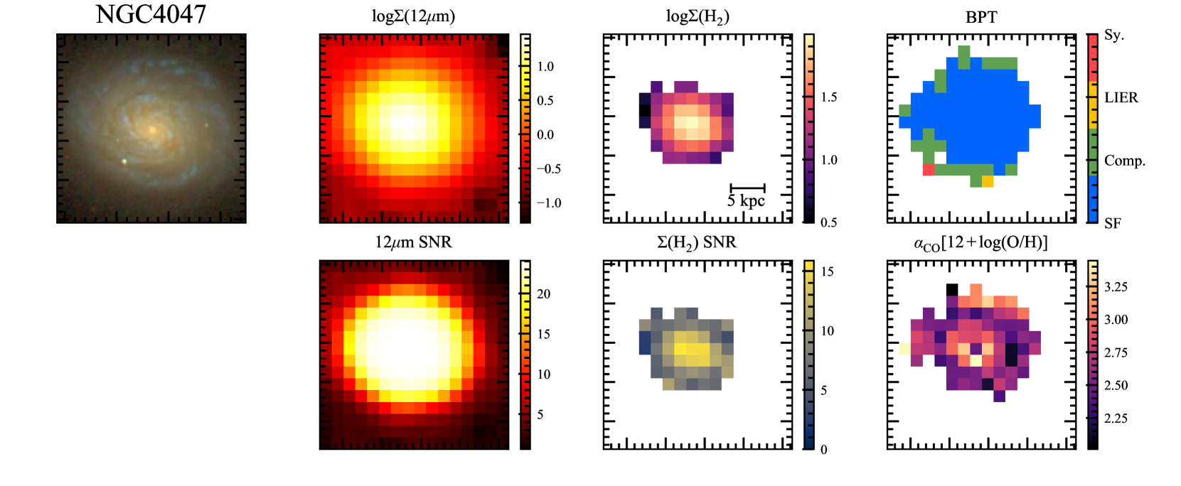
Figure 1: Selected maps for an example galaxy. Top row (left to right): Sloan Digital Sky Survey (SDSS; Blanton et al., 2017) gri thumbnail; WISE 12 µm surface density ($L_{\odot}\>\mathrm{pc^{-2}}$); H₂ mass surface density ($M_{\odot}\>\mathrm{pc^{-2}}$) at 6.6 arcsec resolution and assuming $\alpha_{\mathrm{CO}}=3.2$ $M_{\odot}\>\mathrm{(K\>km\>s^{-1}\>pc^{2})}^{-1}$; BPT diagram for each pixel constructed from the processed CALIFA data (Section 2.4). The pixel size is 6 arcsec, and the cutouts are 96-by-96 arcsec. Bottom row: signal-to-noise ratio (SNR) of the 12 µm and H₂ surface density maps, and the metallicity-dependent $\alpha_{\mathrm{CO}}$ values in units of $M_{\odot}\>\mathrm{(K\>km\>s^{-1}\>pc^{2})}^{-1}$ (Equation 18).

2 Data and Data Processing

2.1 Sample selection

The sample is selected from the EDGE survey (Bolatto et al., 2017, hereafter B17). The typical angular resolution of EDGE CO maps is 4.5 arcsec, and the typical H₂ surface density sensitivity before deprojecting galaxy inclination is 11 $M_{\odot}$ pc^-2 (B17). Every EDGE galaxy has optical integral field unit (IFU) data from CALIFA, allowing joint studies of the content and kinematics of cold gas (H₂), ionized gas, and stellar populations, all with $\sim$kpc spatial resolution. We processed the CO data for all 126 EDGE galaxies, and as a starting point we selected the 95 galaxies which had at least one detected pixel after smoothing to 6.6 arcsec resolution and regridding the moment-0 maps with 6 arcsec pixels (Section 2.3). We then selected those galaxies with inclinations less than 75 degrees, leaving 83 galaxies. Inclination angles were derived from CO rotation curves where available (B17), and otherwise were taken from the HyperLEDA database (Makarov et al., 2014). Redshifts $z$ (from CALIFA emission lines) and luminosity distances $D_{L}$ were taken from B17. A flat $\Lambda$CDM cosmology was assumed ($h=0.7$, $\Omega_{m}=0.27$, $\Omega_{\Lambda}=0.73$).

2.2 WISE 12µm surface density maps

We downloaded 2 degree by 2 degree cutouts (pixel size 1.375 arcsec) of WISE 12 µm (W3) flux $F_{\mathrm{W3}}$ and uncertainty for each galaxy from the NASA/IPAC Infrared Science Archive. The background for each galaxy was estimated using the IDL package Software for Source Extraction (SExtractor; Bertin & Arnouts, 1996), with default parameters and with the corresponding W3 uncertainty map as input. The estimated background was subtracted from each cutout. The background-subtracted images were reprojected with 6 arcsec pixels to avoid over-sampling the 6.6 arcsec beam. These maps were originally in units of Digital Numbers (DN), defined such that a W3 magnitude $m_{\mathrm{W3}}$ of 18.0 corresponds to $F_{\mathrm{W3}}=1.0$ DN, or

$$F_{\mathrm{W3}}=10^{-0.4(m_{\mathrm{W3}}-\mathrm{MAGZP})}\>\mathrm{DN},$$ (3)

where the zero-point magnitude $\mathrm{MAGZP}=18.0$ mag. We converted the maps from their original units to flux density in Jy, given by

$$S_{\mathrm{W3}} =S_{0}10^{-0.4m_{\mathrm{W3}}}$$ (4)

$$=S_{0}10^{-0.4\mathrm{MAGZP}}F_{\mathrm{W3}}$$ (5)

$$=\left(\frac{31.674}{10^{7.2}}\>\mathrm{Jy\>DN^{-1}}\right)F_{\mathrm{W3}}$$ (6)

$$=\left(1.998\times 10^{-6}\>\mathrm{Jy\>DN^{-1}}\right)F_{\mathrm{W3}},$$ (7)

where the isophotal flux density $S_{0}=31.674$ Jy for the W3 band is from Table 1 of Jarrett et al. (2011). Luminosity in units of $\mathrm{L_{\odot}}$ is given by

$$L_{\mathrm{12\>\mu m}} =4\pi D_{L}^{2}\Delta\nu S_{\mathrm{W3}}$$ (8)

$$=7.042F_{\mathrm{W3}}\left(\frac{D_{L}}{\mathrm{Mpc}}\right)^{2}\>\mathrm{L_{\odot}}$$ (9)

where $\Delta\nu=1.1327\times 10^{13}$ Hz is the bandwidth of the 12 µm band (Jarrett et al., 2011), and $D_{L}$ is the luminosity distance. Luminosities were then converted into surface densities $\Sigma(\mathrm{12\>\mu m})$ ($\mathrm{L_{\odot}}$ pc^-2) by

$$\frac{\Sigma(\mathrm{12\>\micron})}{\mathrm{L_{\odot}}\>\mathrm{pc}^{-2}}=7.042\left(\frac{F_{\mathrm{W3}}}{\mathrm{DN}}\right)\left(\frac{D_{L}}{\mathrm{Mpc}}\right)^{2}\left(\frac{A_{\mathrm{pix}}}{\mathrm{pc^{2}}}\right)^{-1}\cos i,$$ (10)

where $i$ is the galaxy inclination, and $A_{\mathrm{pix}}$ is the pixel area in pc².

The uncertainty in each pixel of the rebinned surface density maps is the quadrature sum of the instrumental uncertainty and the 4.5 per cent uncertainty in the zero-point magnitude (Appendix A). Maps for an example galaxy are shown in Figure 1.

2.3 H₂ surface density maps at WISE W3 resolution

The original CO(1-0) datacubes were downloaded from the EDGE website, converted from their native units of K km s^-1 to $\mathrm{Jy\>beam^{-1}\>km\>s^{-1}}$, and then smoothed to a Gaussian beam with FWHM $=6.6$ arcsec using the Common Astronomy Software Applications (CASA; McMullin et al., 2007) task imsmooth to match the WISE resolution. The cubes have a velocity resolution of 20 km s^-1, and span 44 channels (880 km s^-1). Two methods were used to obtain CO integrated intensity (moment-0) maps $S_{\mathrm{CO}}\Delta v$:

1. an iterative masking technique for improving SNR, described in Sun et al. (2018), shown in Figure 1, and

2. integrating the flux along the inner 34 channels (680 km s^-1 total). In this “simple” method, the first 5 and last 5 channels were used to compute the root-mean-square (RMS) noise at each pixel.

Method 1 is used for all results in this work, while Method 2 is used as a cross-check and to estimate upper limits for non-detected pixels.

In Method 1 (described in Sun et al., 2018) a mask is generated for the datacube to improve the signal-to-noise of the resulting moment-0 map. A “core mask” is generated by requiring SNR of 3.5 over 2 consecutive channels (channel width of 20 km s^-1), and a “wing mask” is generated by requiring SNR of 2.0 over 2 consecutive channels. The core mask is dilated within the wing mask to generate a “signal mask” which defines detections. Any detected regions that span an area less than the area of the beam are masked. The signal mask is then extended spectrally by $\pm 1$ channels. Method 2 gives a map with lower signal-to-noise, but is useful for computing upper-limits for pixels which are masked in Method 1, and for cross-checking results.

The moment-0 maps were then rebinned with 6 arcsec pixels, and the units were converted to integrated intensity per pixel

$$\frac{S_{\mathrm{CO}}\Delta v}{\mathrm{Jy\>km\>s^{-1}\>pixel^{-1}}}=\left(\frac{S_{\mathrm{CO}}\Delta v}{\mathrm{Jy\>beam^{-1}\>km\>s^{-1}}}\right)\frac{4\theta_{\mathrm{pix}}^{2}\ln 2}{\pi\mathrm{FWHM}^{2}},$$ (11)

where the beam $\mathrm{FWHM}=6.6$ arcsec, and the pixel size $\theta_{\mathrm{pix}}=6$ arcsec.

The total noise variance in each pixel is the sum in quadrature of the instrumental noise which we assume to be the same for both moment-0 map versions, and calibration uncertainty which depends on the moment-0 method (Appendix B). Instrumental noise maps were computed by measuring the RMS in the first five and final five channels at each pixel (Method 2 above). The instrumental noise maps were rebinned (added in quadrature, then square root) into 6 arcsec pixels. To obtain the total noise for each moment-0 map, a calibration uncertainty of 10 per cent (B17) of the rebinned moment-0 map (both versions described above) was added in quadrature with the instrumental uncertainty. The sensitivity of the CO data is worse than that of WISE W3, and so upper limits for undetected pixels are calculated with the second moment-0 map-making method. All pixels detected at less than 3$\sigma$ in CO were assigned an upper limit of 5 times the noise at each pixel.

The CO(1-0) luminosity and noise maps (in units of K km s^-1 pc²) were computed via (Bolatto et al., 2013)

$$L_{\mathrm{CO(1-0)}}=\frac{2453(S_{\mathrm{CO}}\Delta v)D_{L}^{2}}{1+z},$$ (12)

where $z$ is the redshift. The luminosity maps were converted to H₂-mass surface density $\Sigma(\mathrm{H_{2}})$ using a CO-to-H₂ conversion factor $\alpha_{\mathrm{CO}}$

$$\Sigma(\mathrm{H_{2}})=\frac{\alpha_{\mathrm{CO}}L_{\mathrm{CO}}\cos i}{A_{\mathrm{pix}}},$$ (13)

where $i$ is the galaxy inclination angle, and $A_{\mathrm{pix}}$ is the pixel area in pc². In normal star-forming regions a CO-to-H₂ conversion factor of $\alpha_{\mathrm{CO}}=3.2\>\mathrm{M_{\odot}(K\>km\>s^{-1}\>pc^{2})^{-1}}$ (multiply by 1.36 to include helium) is often assumed (Bolatto et al., 2013). We consider both a constant $\alpha_{\mathrm{CO}}$ and a spatially-varying metallicity-dependent $\alpha_{\mathrm{CO}}$ (Section 2.5).

2.4 Maps of stellar population and ionized gas properties

In the third data release (DR3) of the CALIFA survey there are 667 galaxies observed out to at least two effective radii with $\simeq 2.5$ arcsec angular resolution over wavelengths 3700-7500 Å (Sánchez et al., 2012, 2016). The observations were carried out in either a medium spectral resolution mode (“$V_{1200}$,” $R\simeq 1700$, 3700-4200 Å, 484 galaxies) or a low spectral resolution mode (“$V_{500}$,” $R\simeq 850$, 3750-7500 Å, 646 galaxies). Cubes using data from both $V_{1200}$ and $V_{500}$ were made by degrading the spectral resolution of the $V_{1200}$ cube to that of $V_{500}$ and averaging the spectra where their wavelength coverage overlaps, and using only $V_{1200}$ or $V_{500}$ for the remaining wavelength bins between 3700-7140 Å (Sánchez et al., 2016). Combined $V_{1200}+V_{500}$ datacubes and $V_{500}$ datacubes were downloaded from the CALIFA DR3 webpage. Of the 95 EDGE galaxies detected in CO, combined $V_{1200}+V_{500}$ datacubes are available for 87 galaxies. $V_{500}$ datacubes were used for the remaining 8 galaxies. We refer to this sample of 8 + 87 galaxies as “Sample A” (Table 1).

Table 1: Summary of the number of pixels and galaxies at each stage of sample selection. Note that Samples B and C are selected from Sample A. Sample C is the starting point for Section 3.2 onwards.

Sample label	Criteria	# pixels	# galaxies	Where used
A	At least one CO-detected pixel,⋆ and have $V_{500}+V_{1200}$ or just $V_{500}$ CALIFA datacubes	2317†	95
B	A $\cap$ Have at least 4 CO-detected pixels per galaxy and inclination $i<75\deg^{\ddagger}$	2059	83	Figures 3, 10
C	A $\cap$ Have at least 4 CO-detected pixels classified as star-forming per galaxy and $i<75\deg$	1168	64	Figures 2, 3, 4, 5, 8
⋆ Using Method 1 (Section 2.3).
† CO-detected pixels only.
‡ The reduction in the number of pixels and galaxies when going from Sample A to Sample B is entirely from the inclination cut.

The native pixel size of a CALIFA cube is 1 arcsec. The spaxels were stacked into 6 arcsec spaxels to be compared with the WISE and EDGE CO data. Spectral fitting was performed on the stacked spectra using the Penalized Pixel-Fitting (pPXF) Python package (Cappellari, 2017) to obtain 2D maps of emission and absorption line fluxes, equivalent widths, and velocity dispersions, as well as stellar population properties such as stellar mass and light-weighted stellar age. A Kroupa initial mass function (IMF) was assumed (Kroupa & Weidner, 2003).

Line fluxes were corrected for extinction using the Balmer decrement. Stellar mass was measured from the datacubes after subtracting a dust extinction curve using the method of Li et al. (2020). The unattenuated H$\alpha$ emission line flux $F_{\mathrm{H\alpha}}$ is related to the observed (attenuated) flux according to

$$F_{\mathrm{H\alpha}}=F_{\mathrm{H\alpha,obs.}}10^{0.4A_{V}}$$ (14)

where the extinction is given by

$$A_{V}=5.86\log\left(\frac{F_{\mathrm{H\alpha,obs.}}}{2.86F_{\mathrm{H\beta,obs.}}}\right),$$ (15)

and $F_{\mathrm{H\alpha,obs.}}$ and $F_{\mathrm{H\beta,obs.}}$ are the observed (attenuated) line fluxes. The star formation rate (SFR) surface density is given by

$$\Sigma(\mathrm{SFR}) =\frac{C_{\mathrm{SFR,H\alpha}}L_{\mathrm{H\alpha}}}{A_{\mathrm{pix}}}$$ (16)

$$=\frac{C_{\mathrm{SFR,H\alpha}}F_{\mathrm{H\alpha}}4\pi d^{2}\cos i}{A_{\mathrm{pix}}},$$ (17)

where the H$\alpha$ luminosity-to-SFR calibration factor $C_{\mathrm{SFR,H\alpha}}=5.3\times 10^{-42}\frac{M_{\odot}\>\mathrm{yr}^{-1}}{\mathrm{erg\>s^{-1}}}$ (Hao et al., 2011; Murphy et al., 2011; Kennicutt & Evans, 2012), $d$ is the luminosity distance in cm, and $A_{\mathrm{pix}}$ is the pixel area in kpc².

The mechanism of gas ionization at each pixel was classified as either star formation (SF), low-ionization emission region (LIER), Seyfert (Sy) or a combination of star formation and AGN (“composite”) on a Baldwin, Phillips, and Terlevich (BPT) diagram (Baldwin et al., 1981). It is important to identify non-starforming regions, especially when estimating SFR from H$\alpha$ flux. BPT classification (Figure 1) was done in the [O iii] $\lambda 5007$/H$\beta$ vs. [N ii] $\lambda 6584$/H$\alpha$ plane using three standard demarcation curves in this space: Eq. 5 of Kewley et al. (2001), Eq. 1 of Kauffmann et al. (2003), and Eq. 3 of Cid Fernandes et al. (2010) (see Figure 7 of Husemann et al., 2013).

2.5 CO-to-H₂ conversion factor

The CO-to-H₂ conversion factor $\alpha_{\mathrm{CO}}$ increases slightly with decreasing metallicity (Maloney & Black, 1988; Wilson, 1995; Genzel et al., 2012; Bolatto et al., 2013). At lower metallicities, and consequently lower dust abundance (Draine et al., 2007) and dust shielding, CO is preferentially photodissociated relative to H₂. This process leads to an increase in $\alpha_{\mathrm{CO}}$ (Bolatto et al., 2013).

A metallicity-dependent $\alpha_{\mathrm{CO}}$ equation (Genzel et al., 2012) was calculated at each star-forming pixel (Figure 1)

$$\log\left(\frac{\alpha_{\mathrm{CO}}}{\mathrm{M_{\odot}}\mathrm{(K\>km\>s^{-1}\>pc^{2})^{-1}}}\right)=a+b[12+\log(\mathrm{O/H})],$$ (18)

where $a=12\pm 2$, and $b=-1.30\pm 0.25$. Gas-phase metallicity $12+\log(\mathrm{O/H})$ was computed for the star-forming pixels using

$$12+\log(\mathrm{O/H})=p+q\log\left(\frac{\mathrm{[\text{N\,{ii}}]}\>\lambda 6584}{\mathrm{H\alpha}}\right),$$ (19)

where $p=9.12\pm 0.05$, and $q=0.73\pm 0.10$ (Denicoló et al., 2002). Following other works that have used this $\alpha_{\mathrm{CO}}(Z)$ relation (e.g. Genzel et al., 2015; Tacconi et al., 2018; Bertemes et al., 2018), we consciously choose not to include the uncertainty on $\alpha_{\mathrm{CO}}(Z)$ (which comes from the uncertainties in $a$, $b$, $p$, and $q$) in our analysis, so that the uncertainties on $\log\Sigma(\mathrm{H_{2}})$ only reflect measurement and calibration uncertainties and not systematic uncertainties in the conversion factor.

The metallicity-dependent $\alpha_{\mathrm{CO}}=\alpha_{\mathrm{CO}}(Z)$ (Eq. 18) is our preferred $\alpha_{\mathrm{CO}}$ because it is the most physically accurate. This choice of $\alpha_{\mathrm{CO}}$ has two effects on the sample:

1. the exclusion of non-starforming pixels; and

2. galaxies that have fewer star-forming pixels with CO detections than a given threshold are removed from the sample.

To assess the impacts of these effects, three $\alpha_{\mathrm{CO}}$ scenarios are considered:

1. $\alpha_{\mathrm{CO}}=3.2$, using all pixels (star-forming or not);

2. $\alpha_{\mathrm{CO}}=3.2$, only using star-forming pixels; and

3. a metallicity-dependent $\alpha_{\mathrm{CO}}=\alpha_{\mathrm{CO}}(Z)$ (Eq. 18).

The impact of only considering star-forming pixels on the total number of pixels and galaxies (Table 1) varies depending on how many pixels per galaxy are required. For example, starting from the 95 galaxies in Sample A (Table 1), if we require at least 4 CO-detected pixels per galaxy, our sample will consist of 83 galaxies and 2059 pixels (Sample B). If we require at least 4 CO-detected star-forming pixels per galaxy (e.g. to apply a metallicity-dependent $\alpha_{\mathrm{CO}}$), we would have to remove 43% of the pixels and 22% of the galaxies from the sample, and would be left with 1168 pixels and 64 galaxies (Sample C). In the analysis that follows, we use Sample C exclusively except for comparison with Sample B in Section 3.1.

3 Analysis and Results

3.1 The degree of correlation between $\Sigma(\mathrm{12\>\mu m})$ and $\Sigma(\mathrm{H_{2}})$

Previous work has shown a strong correlation between integrated WISE 12 µm luminosity and CO(1-0) luminosity (Jiang et al., 2015; Gao et al., 2019). To determine if this correlation holds at sub-galaxy spatial scales, we matched the resolution of the EDGE CO maps to WISE W3 resolution and compared surface densities pixel-by-pixel for each galaxy (Figure 2). This comparison indicates that there is a clear correlation between $\Sigma(\mathrm{12\>\mu m})$ and $\Sigma(\mathrm{H_{2}})$, and that within galaxies, the correlation is strong.

To quantify the strength of the correlation per galaxy, the Pearson correlation coefficient between $\log\Sigma(\mathrm{12\>\micron})$ and $\log\Sigma(\mathrm{H_{2}})$ was calculated for each galaxy. The distribution of correlation coefficients across all galaxies was computed separately for each $\alpha_{\mathrm{CO}}$ scenario (Section 2.5; Figure 3). The means for the three distributions are:

1. 0.79 for $\alpha_{\mathrm{CO}}=3.2$, all pixels included;

2. 0.79 for $\alpha_{\mathrm{CO}}=3.2$, star-forming pixels only; and

3. 0.76 for $\alpha_{\mathrm{CO}}(Z)$ (Eq. 18).

These results indicate that there are strong correlations between $\Sigma(\mathrm{12\>\mu m})$ and $\Sigma(\mathrm{H_{2}})$ regardless of the $\alpha_{\mathrm{CO}}$ assumed. A minority of galaxies show poor correlations (4 out of 95 galaxies with correlation coefficients $<0.2$). Reasons for poor correlations include fewer CO-detected pixels, and small dynamic range in the pixels that are detected (e.g. a region covering multiple pixels with uniform surface density).

For comparison, cumulative histograms of the correlation coefficients between $\log\Sigma_{\mathrm{SFR}}$ (Eq. 16) and $\log\Sigma(\mathrm{H_{2}})$ were computed (right panel of Figure 3). The same sets of galaxies and pixels were used as in the left panel of Figure 3, except the “$\alpha_{\mathrm{CO}}=3.2$, all pix.” version is excluded, because $\log\Sigma_{\mathrm{SFR}}$ can only be calculated in star-forming pixels. The mean and median correlation coefficients are lower than those in the left panel of Figure 3. Since the same pixels are used, this suggests a stronger correlation between $\Sigma(\mathrm{12\>\mu m})$ and $\Sigma(\mathrm{H_{2}})$ than between $\Sigma_{\mathrm{SFR}}$ and $\Sigma(\mathrm{H_{2}})$.

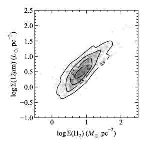
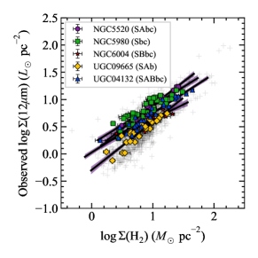
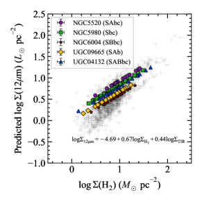
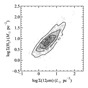
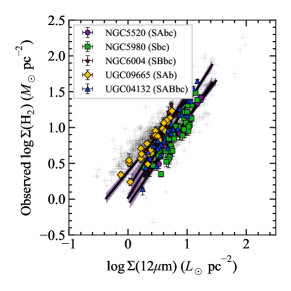
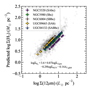
Figure 2: 12 µm surface density versus H₂ surface density (top) and vice versa (bottom) assuming a metallicity-dependent $\alpha_{\mathrm{CO}}$ (Section 2.5). Only star-forming pixels that are detected in CO are shown. Left: The grey points are all pixels, and the fraction of pixels enclosed by each contour are indicated. The grey points are the same in all panels. Middle: Observed values of $\log\Sigma(\mathrm{12\>\mu m})$ (top) and $\log\Sigma(\mathrm{H_{2}})$ (bottom) are shown on the y-axes. The pixel values and best linear fits for five example galaxies from Sample C (Table 1) are coloured to illustrate some of the variation in the correlations found. Hubble types from CALIFA DR3 are indicated in the legend for the five selected galaxies. Right: Predicted values are shown on the y-axes using selected multi-parameter estimators (Table 3). The predictions were made from fits to the pixels from all galaxies except for the galaxy being predicted, to mimic the case where these estimators would be used on a galaxy outside of the sample in this work.

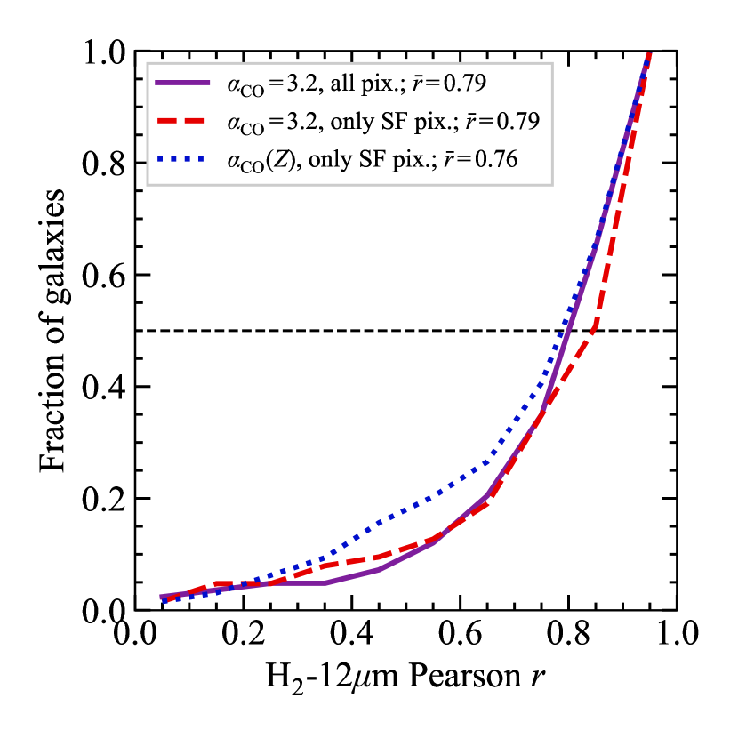
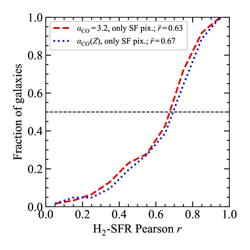
Figure 3: Left: Cumulative histogram of the Pearson correlation coefficient between $\log\Sigma(\mathrm{H_{2}})$ and $\log\Sigma(12\>\micron)$ for each galaxy with a minimum of 4 CO-detected pixels each. Right: Same as left except between $\log\Sigma(\mathrm{H_{2}})$ and $\log\Sigma_{\mathrm{SFR}}$. The three colours are for different $\alpha_{\mathrm{CO}}$ assumptions: (1) $\alpha_{\mathrm{CO}}=3.2$ and including all pixels, (2) $\alpha_{\mathrm{CO}}=3.2$ including only star-forming pixels, and (3) metallicity-dependent $\alpha_{\mathrm{CO}}$ (Eq. 18). There are 83, 64, and 64 galaxies shown in the purple, red, and blue histograms respectively. A strong correlation is found for most galaxies, for each $\alpha_{\mathrm{CO}}$ assumption; however, the mean and median correlations between $\Sigma_{\mathrm{SFR}}$ and $\Sigma(\mathrm{H_{2}})$ are not as strong as those between $\Sigma(\mathrm{12\>\mu m})$ and $\Sigma(\mathrm{H_{2}})$. The same galaxies and pixels were used in both panels, so the differences are not due to a selection effect.

3.2 Bayesian linear regression

The relationship between 12 µm and CO emission resembles the Kennicutt-Schmidt relation, which also shows variation from galaxy to galaxy (Shetty et al., 2013). We model the relationship between $\log\Sigma(\mathrm{12\>\micron})$ and $\log\Sigma(\mathrm{H_{2}})$ with a power-law

$$\log\Sigma(\mathrm{H_{2}})=N\log\Sigma(\mathrm{12\>\micron})+\log C.$$ (20)

To determine whether the 12 µm-CO relation is universal or not, we performed linear fits of $\log\Sigma(\mathrm{H_{2}})$ against $\log\Sigma(12\>\micron)$ for each galaxy with at least 4 CO-detected star-forming pixels (Sample C in Table 1; middle panel of Figure 2). A metallicity-dependent $\alpha_{\mathrm{CO}}$ was used in Figure 2. These fits were performed using LinMix, a Bayesian linear regression code which incorporates uncertainties in both $x$ and $y$ (Kelly, 2007). We repeated the fits for each $\alpha_{\mathrm{CO}}$ (Sec. 2.5) and with $\log\Sigma(\mathrm{H_{2}})$ on the x-axis instead.

For a given galaxy, the best-fit parameters do not vary much depending on the $\alpha_{\mathrm{CO}}$ assumed, provided there are enough pixels to perform the fit even after excluding non-starforming pixels. The fit parameters are also not significantly different if we include upper limits in the fitting. However, we find significant differences in the slope and intercept from galaxy to galaxy, indicating a non-universal resolved relation. The galaxy-to-galaxy variation in best-fit parameters persists for all three $\alpha_{\mathrm{CO}}$ scenarios. The galaxy-to-galaxy variation can be seen in the distribution of slopes and intercepts assuming a metallicity-dependent $\alpha_{\mathrm{CO}}$ for example (Figure 4). The best-fit intercepts span a range of $\simeq 1$ dex ($-0.31$ to $0.87$, median $0.41$), and the slopes range from 0.20 to 2.03, with a median of 1.13. To quantify the significance of the galaxy-to-galaxy variation in best-fit parameters, residuals in the parameters relative to the mean parameters were computed. For example, if the measurement of the slope for galaxy $i$ is $N_{i}\pm\sigma_{N_{i}}$, the residual relative to the average slope over all galaxies $\bar{N}$ is $(N_{i}-\bar{N})/\sigma_{N_{i}}$. Similarly, if the measurement of the intercept for galaxy $i$ is $\log C_{i}\pm\sigma_{\log C_{i}}$, the residual relative to the average intercept over all galaxies $\overline{\log C}$ is $(\log C_{i}-\overline{\log C})/\sigma_{\log C_{i}}$. The residual histograms (Figure 4) show that most of the slopes $N_{i}$ are within $\simeq 1.5\sigma_{N_{i}}$ of $\bar{N}$, but the intercepts show more significant deviations (many beyond $3\sigma_{\log C_{i}}$).

To establish how well-fit all pixels are to a single model, linear fits were done on all CO-detected pixels from all 83 galaxies in Sample B (Table 1) using LinMix (black crosses in Figure 5). The fits were done separately for luminosities ($\log L_{\mathrm{12\>\mu m}}$, $\log L_{\mathrm{CO}}$; left panel of Figure 5) and surface densities ($\log\Sigma(\mathrm{12\>\mu m})$, $\log\Sigma(\mathrm{H_{2}})$; right panel of Figure 5). For completeness, the fits were also done with CO/H₂ on the x-axis (Figure 9). In all cases there are strong correlations (correlation coefficients of $\simeq 0.90$), and good fits (total scatter about the fit $\sigma_{\mathrm{tot}}\simeq 0.19$ dex). By comparing the total scatter $\sigma_{\mathrm{tot}}$ and intrinsic scatter $\sigma_{\mathrm{int}}$ (Appendix C), it is clear that most of the scatter is intrinsic rather than due to measurement and calibration uncertainties. Note that in the right hand panel of Figure 5, ignoring the $\alpha_{\mathrm{CO}}$ uncertainty means that the $\Sigma(\mathrm{H_{2}})$ uncertainty has been underestimated, and therefore the intrinsic scatter $\sigma_{\mathrm{int}}$ (derived from $\sigma_{\mathrm{tot}}$ and the uncertainty on $\Sigma(\mathrm{H_{2}})$, Equation 36) has been overestimated. Also, if we replace $\Sigma(\mathrm{H_{2}})$ with $\Sigma(\mathrm{CO})$, $\sigma_{\mathrm{tot}}$ decreases by only 0.01 dex and $\sigma_{\mathrm{int}}$ does not change, which indicates that the scatter is dominated by that of the 12 µm-CO surface density relationship. Consequently, $\sigma_{\mathrm{int}}$ in the right hand panel of Figure 5 should be interpreted as the intrinsic scatter in the 12 µm-CO surface density relationship.

Similarly, to establish how well-fit all global values are to a single model, linear fits were done on the galaxy-integrated values (green diamonds in Figure 5) for all 83 galaxies in Sample B (Table 1). The results show good fits overall (correlation coefficients of $\simeq 0.90$, scatter about the fit $\sigma_{\mathrm{tot}}\simeq 0.20$ dex). The global values do indeed follow uniform trends (with the exception of one outlier), and the global fits with molecular gas on the x-axis show steeper slopes and smaller y-intercepts than the pixel fits (Figure 5). The global fits with 12 µm on the x-axis show shallower slopes and larger y-intercepts than the pixel fits.

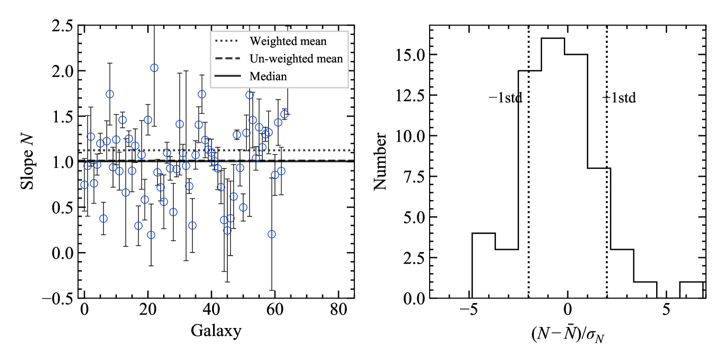
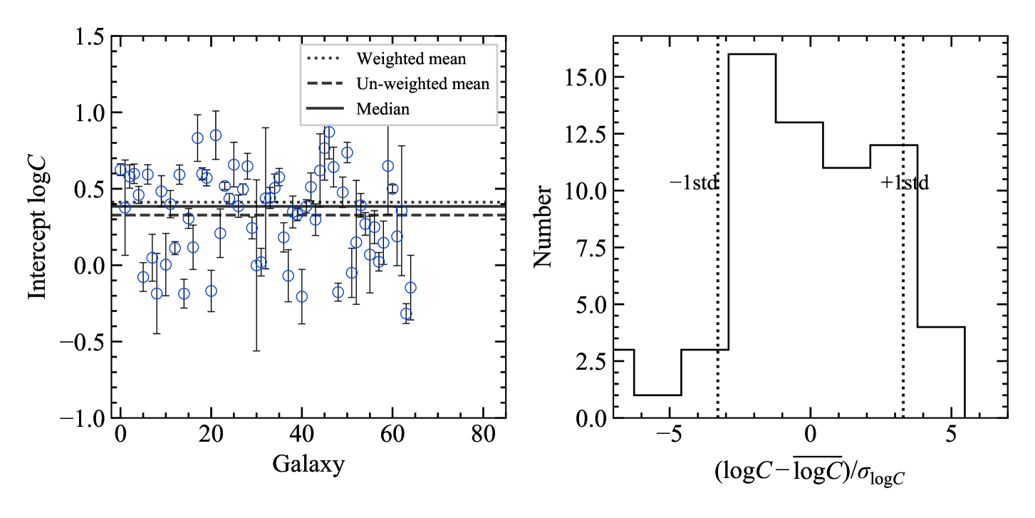
Figure 4: Best-fit slope $N$ (top) and intercept $\log C$ (bottom) of fits to individual pixel measurements of $\log\Sigma(\mathrm{12\>\mu m})$ (x-axis) versus $\log\Sigma(\mathrm{H_{2}})$ (y-axis). Each point is for one galaxy. A metallicity-dependent $\alpha_{\mathrm{CO}}$ was used, so only star-forming pixels were used in the fits. At least 4 CO-detected star-forming pixels per galaxy were required (Sample C, Table 1). Left: The horizontal lines show the inverse-variance weighted means (dotted), un-weighted means (solid), and medians (dashed). Right: Histograms of the residuals for each galaxy relative to the weighted mean, divided by the uncertainty for each galaxy. The vertical lines indicate $\pm 1$ times the standard deviation of each distribution.

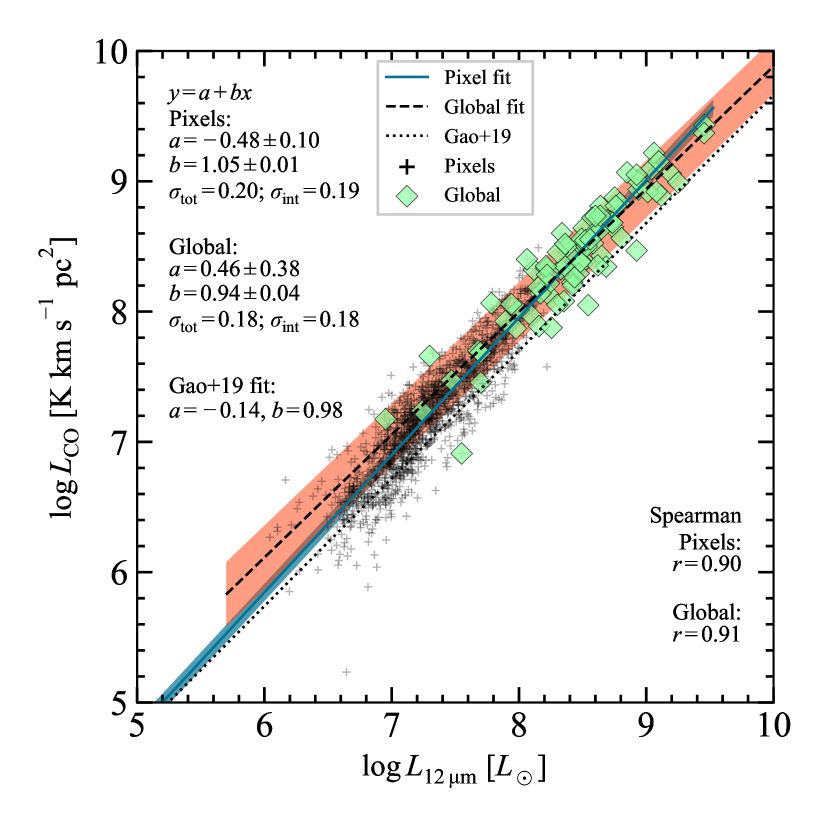
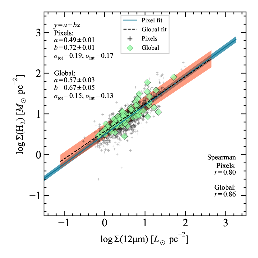
Figure 5: Measurements of 12 µm and H₂ (or CO) using all individual pixels from all galaxies in the sample (black crosses), and the galaxy-integrated values (diamonds). The fits (Section 3.2) were done separately for the pixel measurements (blue regions) and the global measurements (red regions). Best-fit parameters assuming a power-law model (Equation 20), and the total $\sigma_{\mathrm{tot}}$ and intrinsic $\sigma_{\mathrm{int}}$ scatter (Appendix C) about the fits are indicated. The left and right panels show the fits to luminosities and surface densities respectively. H₂ surface densities were calculated using a metallicity-dependent $\alpha_{\mathrm{CO}}$ (Equation 18). Note that in the right hand panel, ignoring $\alpha_{\mathrm{CO}}$ uncertainty means that the $\Sigma(\mathrm{H_{2}})$ uncertainty has been underestimated, and therefore the intrinsic scatter $\sigma_{\mathrm{int}}$ (derived from $\sigma_{\mathrm{tot}}$ and the uncertainty on $\Sigma(\mathrm{H_{2}})$, Equation 36) has been overestimated. Also, if we replace $\Sigma(\mathrm{H_{2}})$ with $\Sigma(\mathrm{CO})$, $\sigma_{\mathrm{tot}}$ decreases by only 0.01 dex and $\sigma_{\mathrm{int}}$ does not change, which indicates that the scatter is dominated by that of the 12 µm-CO surface density relationship. Consequently, $\sigma_{\mathrm{int}}$ in the right panel should be interpreted as the intrinsic scatter in the 12 µm-CO surface density relationship. For completeness, versions of these plots using the same data but with the x and y axes interchanged are shown in Figure 9, and versions with a constant $\alpha_{\mathrm{CO}}$ and non-starforming pixels included are shown in Figure 10.

3.3 Spatially resolved estimator of $\Sigma(\mathrm{H_{2}})$

To develop an estimator of $\log\Sigma(\mathrm{H_{2}})$ from $\log\Sigma(\mathrm{12\>\mu m})$ and other galaxy properties, we performed linear regression on all of the star-forming pixels from all galaxies combined. Global properties (from UV, optical, and infrared measurements) and resolved optical properties were included (Table 2). The model is

$$\vec{y}=\theta_{0}+\sum_{i}\theta_{i}\vec{x_{i}},$$ (21)

where each entry of $\vec{y}$ is $\log\Sigma(\mathrm{H_{2}})$ for each pixel of each galaxy (using the metallicity-dependent $\alpha_{\mathrm{CO}}$, Eq. 18), the $\theta$ are the fit parameters, and the sum is over $i$ properties (a combination of pixel properties or global properties). We used ridge regression, implemented in the Scikit-Learn Python package (Pedregosa et al., 2012), which is the same as ordinary least squares regression except it includes a penalty in the likelihood for more complicated models. The penalty term is the sum of the squared coefficients of each parameter $\delta\sum_{i}\theta_{i}^{2}$. The regularization parameter $\delta$ (a scalar) sets the impact of the penalty term. The best value of $\delta$ was determined by cross-validation using RidgeCV. In ridge regression it is important to standardize the data prior to fitting (subtract the sample mean and divide by the standard deviation for all global properties and pixel properties) so that the penalty term is not affected by different units or spreads of the properties. The standardized version of Equation 21 is

$$\vec{y}-\mathrm{mean}(\vec{y})=\sum_{i}\tilde{\theta_{i}}\left[\frac{\vec{x_{i}}-\mathrm{mean}(\vec{x_{i}})}{\mathrm{std}(\vec{x_{i}})}\right].$$ (22)

Note that it is not necessary to divide $\vec{y}-\mathrm{mean}(\vec{y})$ by $\mathrm{std}(\vec{y})$ because it does not impact the regularization term. After performing ridge regression on the standardized data (which provides $\tilde{\theta_{i}}$), the best-fit coefficients in the original units are given by

$$\theta_{i}=\frac{\tilde{\theta_{i}}}{\mathrm{std}(\vec{x_{i}})}.$$ (23)

The intercept $\theta_{0}$ is given by

$$\theta_{0}=\mathrm{mean}(\vec{y})-\sum_{i}\tilde{\theta_{i}}\left[\frac{\mathrm{mean}(\vec{x_{i}})}{\mathrm{std}(\vec{x_{i}})}\right].$$ (24)

Table 2: Global properties (top) and pixel properties (bottom) considered in the multi-parameter fits (Section 3.3). The SFR and stellar masses from  B17 were both multiplied by 0.66 to convert from Salpeter to Kroupa IMF (Madau & Dickinson, 2014). Global SFR, $M_{*}$, and luminosities were converted to surface densities by dividing by $2\pi r_{50}^{2}$, where $r_{50}$ is the i-band half-light radius in kpc from Gilhuly & Courteau (2018).

Label	Units	Reference	Description
Global Properties
$12+\log\mathrm{O/H}_{\mathrm{glob}}$	dex	B17	[O iii]/[N ii]-based gas-phase metallicity
$\log\Sigma_{\mathrm{SFR,glob}}$	$\mathrm{M_{\odot}}$ yr-1 kpc-2	B17	Star formation rate surface density ($5.3\times 10^{-42}L(\mathrm{H\alpha})/2\pi r_{50}^{2}$)
$\log\Sigma_{\mathrm{*,glob}}$	$\mathrm{M_{\odot}}$ kpc-2	B17	Stellar mass surface density assuming a Kroupa IMF
$\log\cos i$		B17	Inclination $i$ is either from CO kinematics, H$\alpha$ kinematics, or LEDA
$\log\Sigma_{\mathrm{NUV}}$	1042 erg s-1 kpc-2	C15	Near-UV surface density
$\log\Sigma_{\mathrm{FUV}}$	1042 erg s-1 kpc-2	C15	Far-UV surface density
$\log\Sigma_{\mathrm{TIR}}$	1043 erg s-1 kpc-2	C15	Total-IR (8-1000µm) surface density
$\log\Sigma_{\mathrm{W4}}$	1042 erg s-1 kpc-2	C15	WISE W4 (22 µm) surface density
$u-r$	mag	B17	Colour from CALIFA synthetic photometry (SDSS filters applied to extinction-corrected spectra)
$b/a$		C15	Minor-to-major axis ratio from CALIFA synthetic photometry
$(B/T)_{g}$		C15	Bulge-to-total ratio from $g$-band photometry
$n_{g}$		C15	Sérsic index from $g$-band photometry
$\log\sigma_{\mathrm{bulge}}$	km s-1	G19	Bulge velocity dispersion (5 arcsec aperture)
$A_{V,\mathrm{glob}}$	mag	C15	Extinction measured from the Balmer decrement
Pixel Properties
$12+\log\mathrm{O/H}_{\mathrm{pix}}$	dex	Eq. 19	[O iii]/[N ii]-based gas-phase metallicity
$\log\Sigma_{\mathrm{SFR,pix}}$	$\mathrm{M_{\odot}}$ yr-1 kpc-2	Eq. 16	Star formation rate surface density
$\log\Sigma_{\mathrm{*,pix}}$	$\mathrm{M_{\odot}}$ pc-2	Sec. 2.4	Stellar mass surface density, assuming a Kroupa IMF
$A_{V,\mathrm{pix}}$	mag	Eq. 15	Extinction measured from the Balmer decrement

Our goal was to identify a combination of properties such that the linear fit of $\log\Sigma(\mathrm{H_{2}})$ vs. these properties (including $\log\Sigma(\mathrm{12\>\mu m})$) was able to reliably predict $\log\Sigma(\mathrm{H_{2}})$. The $\log\Sigma(\mathrm{H_{2}})$-predicting ability of the fit to a given parameter combination was quantified by performing fits with one galaxy excluded, and then measuring the mean-square (MS) error of the prediction for the excluded galaxy (the “testing error”)

$$\mathrm{MS\>error}=\frac{1}{N_{\mathrm{pix}}}\sum_{N_{\mathrm{pix}}}(y_{\mathrm{true}}-y_{\mathrm{pred}})^{2},$$ (25)

where $N_{\mathrm{pix}}$ is the number of pixels for this galaxy, $y_{\mathrm{true}}$ is the true value of $\log\Sigma(\mathrm{H_{2}})$ in each pixel, and $y_{\mathrm{pred}}$ is the predicted value at that pixel using the fit. The RMS error over all test galaxies

$$\mathrm{RMS\>error}=\sqrt{\frac{1}{N_{\mathrm{galaxies}}}\sum_{\mathrm{galaxy}}\mathrm{MS\>error}_{\mathrm{galaxy}}}$$ (26)

was used to decide on a best parameter combination.

To identify the best possible combination of parameters we did the fit separately for all possible combinations with at least one resolved property required in each combination. We did not want to exclude the possibility of parameters other than 12 µm being better predictors of H₂, so we included all combinations even if 12 µm was excluded. To avoid overfitting, we excluded galaxies if the number of CO-detected star-forming pixels minus the number of galaxy properties in the estimator was less than 4 (so there are at least 3 degrees of freedom per galaxy after doing the fit), and only considered models with less than 6 independent variables. We used the metallicity-dependent $\alpha_{\mathrm{CO}}$, so the sample used for these fits was Sample C (Table 1); however, depending on the number of galaxy properties used and the number of CO-detected star-forming pixels, the sample is smaller for some estimators. We require a minimum of 15 galaxies for each estimator.

Here we describe how the pixel selection and fitting method were used to calculate the RMS error for each combination of galaxy properties:

1. Generate all possible sets of pixels such that each set has the pixels from one galaxy left out.

2. For each set of pixels:

   1. Compute $\mathrm{mean}(\vec{x_{i}})$ and $\mathrm{std}(\vec{x_{i}})$ of the resolved and global properties $\vec{x_{i}}$. Use these to standardize the data.

   2. Perform the multi-parameter fit on the standardized data, which yields $\tilde{\theta_{i}}$ (Eq. 22).

   3. Compute the un-standardized coefficients $\theta_{i}$ (Eq. 23) and zero-point $\theta_{0}$ (Eq. 24).

   4. Use these $\theta_{0}$, $\theta_{i}$ to predict $\vec{y}$ of the excluded galaxy (Eq. 21).

   5. Tabulate the mean squared-error (Eq. 25).

3. Compute the RMS error (Eq. 26) from all of the MS errors. This indicates the ability of this multi-parameter fit to predict new $\vec{y}$. The RMS error for each estimator is shown in Figure 6.

In practical applications outside of this work, not all of the global properties and pixel properties will be available. For this reason, we provide several $\log\Sigma(\mathrm{H_{2}})$ estimators which can be used depending on which data are available. To highlight the relative importance of resolved optical properties vs. 12 µm, the best-performing estimators based on the following galaxy properties are compared:

1. all global properties + IFU properties + 12 µm (Table 3),

2. all global properties + 12 µm but no IFU properties (Table 4),

3. all global properties + IFU properties but no 12 µm (Table 5).

The performance of the estimators was ranked based on their RMS error of predicted $\log\Sigma(\mathrm{H_{2}})$ (Figure 6). The reported estimators are those with the lowest RMS error at a given number of galaxy properties (those corresponding to the stars and squares in Figure 6). We estimated the uncertainty on the coefficients in each estimator by perturbing the 12 µm and H₂ data points randomly according to their uncertainties, redoing the fits 1000 times, and measuring the standard deviation of the parameter distributions.

The lack of points below the green curve in Figure 6 indicates that there is little to be gained by adding IFU data to the estimators with resolved 12 µm (little to no drop in RMS error). The RMS error of the estimator with only resolved $A_{V}$ for example (black circle, upper left) performs significantly worse than the fit with only 12 µm (green square, lower left). Estimators with resolved 12 µm but no IFU data perform better than those with IFU data but no resolved 12 µm. There is also no improvement in predictive accuracy of the estimators using global properties + resolved 12 µm + no IFU data beyond a four-parameter fit (intercept, $\Sigma(12\mathrm{\mu m})$, $\Sigma_{\mathrm{NUV}}$, and global $A_{V}$). The best H₂ estimators all contain $\log\Sigma(\mathrm{12\>\micron})$, which indicates that this variable is indeed the most important for predicting H₂.

For the fits in the opposite direction, $\log\Sigma(\mathrm{H_{2}})$ was found to be the most important for predicting $\mathrm{12\>\micron}$. The best estimators for 1-5 galaxy properties show that if $\log\Sigma(\mathrm{H_{2}})$ is already included, there is essentially no improvement in predictive accuracy (little to no drop in RMS error) when resolved optical IFU data are included as variables in the fitting.

We compared how well these multi-parameter estimators perform relative to the one-parameter estimator from the right panel of Figure 5:

$$\log\Sigma(\mathrm{H_{2}})=(0.49\pm 0.01)+(0.72\pm 0.01)\log\Sigma(12\mathrm{\mu m}).$$ (27)

Note that this fit, obtained via Bayesian linear regression (Sec. 3.2) is consistent with the result from ridge regression (first row of Table 3). To compare the performance of each estimator with the fit above, predicted $\log\Sigma(\mathrm{H_{2}})$ for each pixel was computed from the one-parameter fit, and the RMS error (square root of Eq. 25) was computed for each galaxy (Figure 7). Most points lie below the 1:1 relation in Figure 7, indicating that the multi-parameter fits have lower RMS error per pixel than the single-parameter fit.

Table 3: Best-performing estimators of $\log\Sigma(\mathrm{H_{2}})$ (metallicity-dependent $\alpha_{\mathrm{CO}}$, Sec. 2.5) based on global properties + resolved 12 µm + resolved optical IFU properties (Table 2). Each successive row adds one galaxy property. For example, the estimator in the second row is $\log\Sigma(\mathrm{H_{2}})=2.54+0.78\log\Sigma(\mathrm{12\>\mu m})-0.20\log\Sigma_{\mathrm{FUV}}$. The RMS error (the accuracy of predicted $\log\Sigma(\mathrm{H_{2}})$ per pixel, Eq. 26), the number of galaxies $n_{\mathrm{gal}}$ and pixels $n_{\mathrm{pix}}$ used for the fit, and the intrinsic scatter ($\sigma_{\mathrm{int}}$, Appendix C) are reported. Table 7 shows the best-fit results assuming $\alpha_{\mathrm{CO}}=3.2$.

					$\theta_{i}$ for pixel properties		$\theta_{i}$ for global properties
RMS error	$n_{\mathrm{gal}}$	$n_{\mathrm{pix}}$	$\sigma_{\mathrm{int}}$	Zero-point ($\theta_{0}$)	$\log\Sigma(\mathrm{12\>\mu m})$	$(12+\log\mathrm{O/H})$	$\log\Sigma_{\mathrm{FUV}}$	$\log\Sigma_{\mathrm{NUV}}$	$A(\mathrm{H\alpha})$
$0.19$	$58$	$1126$	$0.17$	$0.48\pm 0.01$	$0.71\pm 0.01$	–	–	–	–
$0.17$	$30$	$573$	$0.15$	$2.54\pm 0.07$	$0.78\pm 0.01$	–	$-0.20\pm 0.01$	–	–
$0.15$	$27$	$552$	$0.15$	$3.6\pm 0.1$	$0.87\pm 0.01$	–	–	$-0.29\pm 0.01$	$-0.14\pm 0.01$
$0.14$	$27$	$552$	$0.14$	$14.6\pm 0.6$	$0.94\pm 0.01$	$-1.24\pm 0.07$	–	$-0.30\pm 0.01$	$-0.15\pm 0.01$

Table 4: Same as Table 3 but the best-performing estimators based on global properties + resolved 12 µm  but no resolved optical IFU properties. Table 8 shows the best-fit results assuming $\alpha_{\mathrm{CO}}=3.2$.

					$\theta_{i}$ for pixel properties	$\theta_{i}$ for global properties
RMS error	$n_{\mathrm{gal}}$	$n_{\mathrm{pix}}$	$\sigma_{\mathrm{int}}$	Zero-point ($\theta_{0}$)	$\log\Sigma(\mathrm{12\>\mu m})$	$\log\Sigma_{\mathrm{FUV}}$	$\log\Sigma_{\mathrm{NUV}}$	$A(\mathrm{H\alpha})$
$0.19$	$58$	$1126$	$0.17$	$0.47\pm 0.01$	$0.71\pm 0.01$	–	–	–
$0.17$	$30$	$573$	$0.15$	$2.54\pm 0.07$	$0.78\pm 0.01$	$-0.20\pm 0.01$	–	–
$0.15$	$27$	$552$	$0.15$	$3.6\pm 0.1$	$0.88\pm 0.01$	–	$-0.29\pm 0.01$	$-0.14\pm 0.01$
$0.15$	$27$	$552$	$0.15$	$3.6\pm 0.1$	$0.87\pm 0.01$	$0.03\pm 0.03$	$-0.31\pm 0.04$	$-0.14\pm 0.01$

Table 5: Same as Table 3 but the best-performing estimators based on global properties + resolved optical IFU properties but no resolved 12 µm. Table 9 shows the best-fit results assuming $\alpha_{\mathrm{CO}}=3.2$.

					$\theta_{i}$ for pixel properties			$\theta_{i}$ for global properties
RMS error	$n_{\mathrm{gal}}$	$n_{\mathrm{pix}}$	$\sigma_{\mathrm{int}}$	Zero-point ($\theta_{0}$)	$\log\Sigma_{*}$	$(12+\log\mathrm{O/H})$	$\log\Sigma_{\mathrm{SFR}}$	$\log\Sigma_{\mathrm{NUV}}$	$b/a_{\mathrm{disk}}$
$0.20$	$58$	$1126$	$0.19$	$2.00\pm 0.01$	–	–	$0.50\pm 0.01$	–	–
$0.20$	$42$	$942$	$0.18$	$1.86\pm 0.01$	–	–	$0.50\pm 0.01$	–	$0.22\pm 0.01$
$0.17$	$27$	$552$	$0.18$	$1.3\pm 0.1$	$0.18\pm 0.01$	–	$0.35\pm 0.01$	$0.01\pm 0.01$	–
$0.17$	$27$	$552$	$0.18$	$8.0\pm 0.6$	$0.23\pm 0.01$	$-0.81\pm 0.07$	$0.32\pm 0.01$	$0.02\pm 0.01$	–

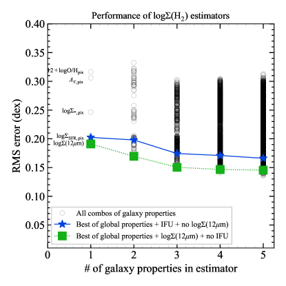
Figure 6: RMS error (Equation 26) of all estimators. Estimators with smaller RMS errors have better predictive accuracy. The RMS error decreases only slightly as the number of independent variables increases for the fits with resolved 12 µm but no IFU data. The fits with resolved 12 µm but no IFU data have lower RMS errors than those with IFU data. The lack of points below the green curve indicates that there is little to be gained by adding IFU data to the estimators with resolved 12 µm. The RMS error of the estimator with only resolved $A_{V}$ for example (black circle, upper left) performs significantly worse than the fit with only 12 µm (green square, lower left).

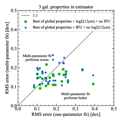
Figure 7: Galaxy-by-galaxy RMS error (Equation 26) computed from the specified multi-parameter fits with 3 galaxy properties, versus the RMS error computed from the one parameter surface density fit (Figure 5). The green squares and blue stars correspond to the green square and blue star in Figure 6 at $n=3$ respectively. The RMS of the y-values of the green squares here gives the RMS error at $n=3$ in Figure 6, and likewise for the blue stars (Equation 26).

3.4 Dependence of the 12 µm-H₂ relationship on physical scale

To establish whether the correlation between global surface densities (12 µm vs H₂) arises from a local correlation between pixel-based surface densities, we computed residuals of the individual pixel measurements from the resolved pixel fit (right panel of Figure 5) with varying surface areas (Figure 8). For each galaxy, contiguous regions of 1, 4, 7 or 9 pixels were used to compute surface densities (the four columns of Figure 8). The contiguous pixels were required to be CO-detected and star-forming, as a metallicity-dependent $\alpha_{\mathrm{CO}}$ was used. Each pixel was used in exactly one surface density calculation for each resolution, so all of the black circles are independent. We found that the scatter diminished as the pixel size approached the whole galaxy size. The total scatter about the individual pixel fit declines as pixel area increases, indicating that the global correlation emerges from the local one.

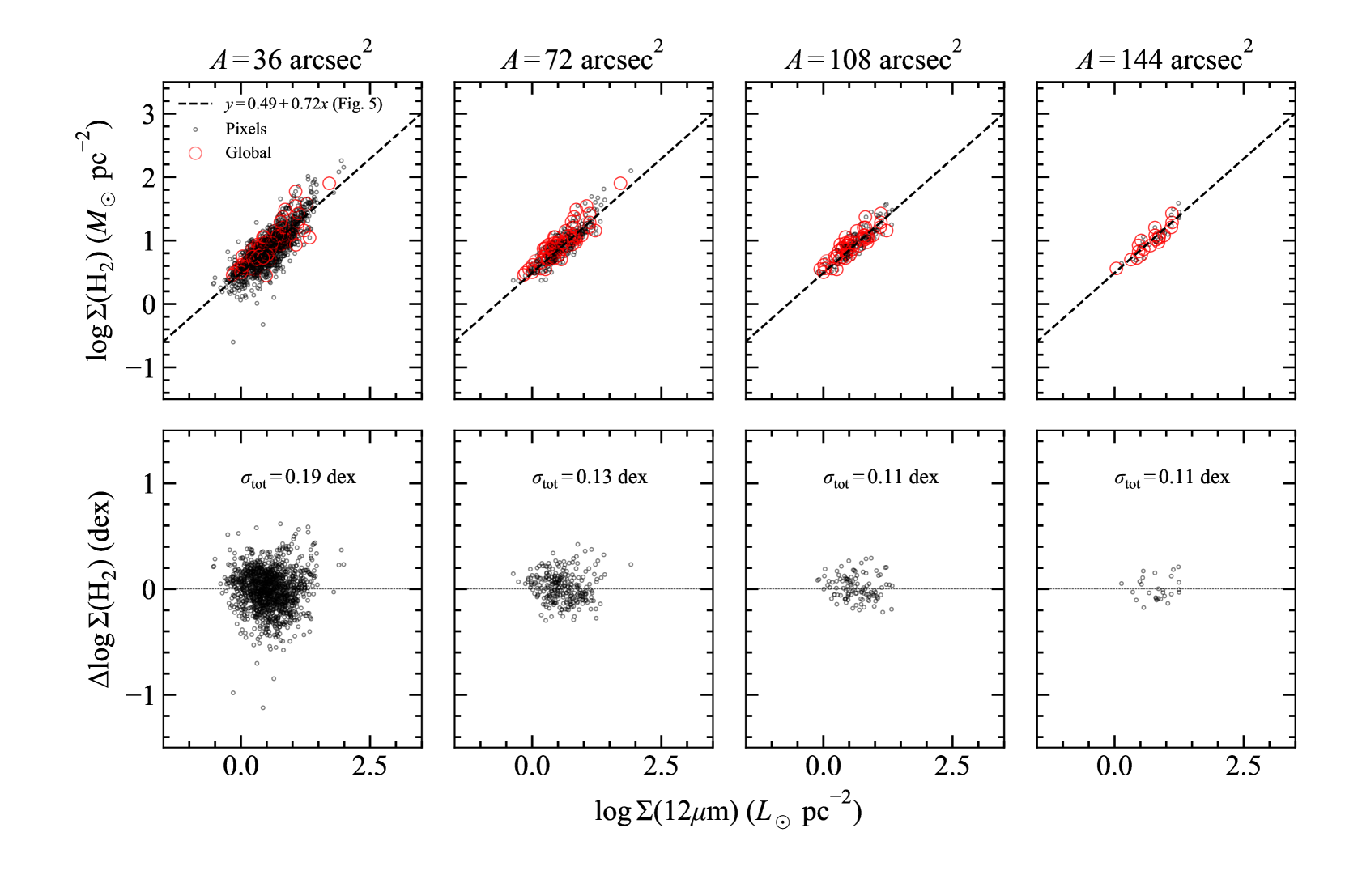
Figure 8: Variation of the scatter in the $\Sigma(\mathrm{H_{2}})$-$\Sigma(\mathrm{12\>\mu m})$ relationship with the area over which surface densities are calculated. Top: black points are surface densities computed over area $A$ indicated at the top (36 arcsec² is one 6 arcsec pixel). Red circles are the sum of all pixels for each galaxy in the sample, and are the same in all panels in which that galaxy appears. The H₂ surface densities are computed with a metallicity-dependent $\alpha_{\mathrm{CO}}$. For each galaxy, all contiguous CO-detected, star-forming pixels with area $A$ were used. Each pixel was used exactly once in each panel from left to right. The number of galaxies decreases from left to right because some galaxies do not have any contiguous pixels which form the specified area. The fit to individual pixels is the same in all panels. Bottom: residuals in 12 µm surface density, relative to the resolved pixel fit (black line) from the bottom right panel of Figure 5. The total scatter $\sigma_{\mathrm{tot}}$ about the resolved fit decreases as the surface area approaches the total galaxy area, suggesting that the global correlation (red circles) emerges from the resolved correlation (black circles).

3.5 Testing the estimators for biases

To determine whether the best-fit relations are biased with respect to any global or resolved properties (Table 2), we performed the following tests for the best-performing H₂ estimators with 1, 2, and 3 parameters from Table 3.

For resolved properties, we plotted the residual in predicted vs. true $\log\Sigma(\mathrm{H_{2}})$ for each pixel versus resolved properties. We computed the Pearson-$r$ between the residuals and the resolved quantities. No significant correlations were found for any of the resolved properties. This indicates that the performance of the estimators is not biased with respect to resolved properties.

For global properties, we plotted the RMS error (Equation 26) for each galaxy versus global properties for that galaxy. We computed the Pearson-$r$ between the RMS error and global quantities. No significant correlations were found for any of the global properties. This indicates that the performance of the estimators is not biased with respect to global properties.

4 Discussion

Our findings show that significant power-law correlations between 12 µm and CO surface densities at kiloparsec scales are responsible for the observed correlation between global (galaxy-wide) measurements (Jiang et al., 2015; Gao et al., 2019). The median correlation coefficient between $\log\Sigma(\mathrm{12\>\micron})$ and $\log\Sigma(\mathrm{H_{2}})$ is $\simeq 0.86$ (per galaxy). Linear fits for each galaxy yield a range of intercepts spanning $\simeq 1$ dex ($-0.31$ to $0.87$, median 0.41), and a range in slopes (0.20 to 2.03, median 1.13). The 12 µm and CO luminosities computed over the CO-detected area of each galaxy in the sample are well-fit by a single power law, with a larger slope and smaller y-intercept than the fit to all individual-pixel luminosities in the sample. Linear regression on all possible combinations of resolved properties and global properties (Table 2) yielded several equations which can be used to estimate $\Sigma(\mathrm{H_{2}})$ (assuming a metallicity-dependent $\alpha_{\mathrm{CO}}$) in individual pixels. A catalog of all resolved and global properties for each pixel in the analysis is provided in machine-readable format (Table 6). The estimators were ranked according to the average accuracy with which they can predict $\Sigma(\mathrm{H_{2}})$ in a given pixel (RMS error, Eq. 26). The best-performing estimators (Tables 3, 4, 5) with 1-4 independent variables are provided, and there is only marginal improvement in prediction error beyond 3 independent variables. Out of all possible parameter combinations considered, the best-performing estimators include resolved $\Sigma(\mathrm{12\>\mu m})$, indicating that 12 µm emission is likely physically linked to H₂ at resolved scales.

Table 6: Selected rows and columns of the catalog of resolved measurements for each pixel considered in the analysis. A full version with more columns and rows is available in machine-readable format. A Python script is provided which shows how to reconstruct two-dimensional images of all quantities in the catalog for each galaxy. The luminosities corresponding to the surface densities in columns 9-12 are provided in the full catalog.

Pixel ID	Galaxy	BPT	$12+\log\mathrm{O/H_{pix}}$	$\alpha_{\mathrm{CO}}$	$\log\Sigma_{*,\mathrm{pix}}$	$\log\Sigma_{\mathrm{SFR,pix}}$	$A_{V,\mathrm{pix}}$	$\log\Sigma_{\mathrm{H_{2}}}$ (Simple)	$\log\Sigma_{\mathrm{H_{2}}}$ (Sun)	$\log\Sigma_{\mathrm{H_{2}}}$ (Sun, $\alpha_{\mathrm{CO}}(Z)$)	$\log\Sigma(\mathrm{12\>\mu m})$
(1)	(2)	(3)	(4)	(5)	(6)	(7)	(8)	(9)	(10)	(11)	(12)
1464	NGC5980	Comp.	–	–	$2.49$	–	–	$1.27\pm 0.06$	$1.24\pm 0.05$	–	$1.09\pm 0.02$
1465	NGC5980	Comp.	–	–	$3.13$	–	–	$1.68\pm 0.05$	$1.70\pm 0.03$	–	$1.21\pm 0.02$
1466	NGC5980	SF	8.83	2.44	$2.48$	$-1.61\pm 0.03$	$1.08$	$1.06\pm 0.11$	$1.13\pm 0.06$	$1.01\pm 0.06$	$1.03\pm 0.02$
1467	NGC5980	SF	8.84	2.40	$1.60$	$-2.10\pm 0.02$	$1.02$	$<1.09$	$0.65\pm 0.07$	$0.52\pm 0.07$	$0.65\pm 0.02$
1468	NGC5980	Comp.	–	–	$0.73$	–	–	$<1.12$	–	–	$0.17\pm 0.02$
1469	NGC5980	SF	8.84	2.39	$-1.04$	$-3.77\pm 0.03$	$-3.02$	$<1.24$	–	–	$-0.29\pm 0.04$
24622	NGC4047	SF	8.80	2.70	$2.30$	$-1.51\pm 0.03$	$1.26$	$1.58\pm 0.09$	$1.61\pm 0.04$	$1.54\pm 0.04$	$1.17\pm 0.02$
24623	NGC4047	SF	8.76	2.97	$2.65$	$-1.30\pm 0.02$	$1.21$	$1.78\pm 0.05$	$1.87\pm 0.03$	$1.83\pm 0.03$	$1.35\pm 0.02$
24624	NGC4047	SF	8.71	3.45	$2.72$	$-1.20\pm 0.02$	$1.08$	$1.88\pm 0.05$	$1.90\pm 0.03$	$1.93\pm 0.03$	$1.41\pm 0.02$
24625	NGC4047	SF	8.76	3.02	$2.46$	$-1.40\pm 0.02$	$1.11$	$1.81\pm 0.07$	$1.81\pm 0.03$	$1.78\pm 0.03$	$1.36\pm 0.02$
24626	NGC4047	SF	8.83	2.47	$2.13$	$-1.65\pm 0.02$	$1.09$	$1.47\pm 0.13$	$1.55\pm 0.04$	$1.43\pm 0.04$	$1.20\pm 0.02$
24627	NGC4047	SF	8.85	2.32	$2.04$	$-1.82\pm 0.03$	$1.28$	$<1.63$	$1.20\pm 0.08$	$1.06\pm 0.08$	$0.96\pm 0.02$
24628	NGC4047	Comp.	–	–	$1.41$	–	–	$<1.63$	–	–	$0.63\pm 0.02$
24629	NGC4047	SF	8.80	2.64	$1.08$	$-3.01\pm 0.09$	$0.50$	$<1.65$	–	–	$0.26\pm 0.03$
24630	NGC4047	–	–	–	–	–	–	$<1.72$	–	–	$-0.06\pm 0.05$
24631	NGC4047	–	–	–	–	–	–	$<1.86$	–	–	$-0.30\pm 0.07$
24632	NGC4047	–	–	–	–	–	–	$<1.71$	–	–	$-0.52\pm 0.12$
24633	NGC4047	–	–	–	–	–	–	$<1.70$	–	–	$-0.31\pm 0.08$
24634	NGC4047	–	–	–	–	–	–	$<1.79$	–	–	$-0.02\pm 0.04$
24635	NGC4047	SF	8.79	2.73	$1.21$	$-2.34\pm 0.05$	$1.12$	$<1.67$	–	–	$0.26\pm 0.03$
24636	NGC4047	SF	8.84	2.36	$1.65$	$-2.45\pm 0.04$	$0.86$	$<1.58$	–	–	$0.55\pm 0.02$
24637	NGC4047	SF	8.88	2.13	$1.90$	$-2.34\pm 0.04$	$0.68$	$<1.58$	$1.16\pm 0.06$	$0.98\pm 0.06$	$0.90\pm 0.02$
(3) BPT classification (Section 2.4): starforming (“SF”), composite (“Comp.”), low-ionization emission region (“LIER”), or Seyfert (“Sy”).
(5) Metallicity-dependent $\alpha_{\mathrm{CO}}$ (Eq. 18) in units of $\mathrm{M_{\odot}}\mathrm{(K\>km\>s^{-1}\>pc^{2})^{-1}}$.
(6) Resolved stellar mass surface density (Sec. 2.4) in units of $\mathrm{M_{\odot}}\>\mathrm{kpc}^{-2}$.
(7) Resolved SFR surface density (Equation 16) in units of $\mathrm{M_{\odot}}\>\mathrm{yr}^{-1}\>\mathrm{kpc}^{-2}$.
(8) Resolved extinction derived from the Balmer decrement, in units of mag (Equation 15).
(9) H2 surface density ($\mathrm{M_{\odot}}\>\mathrm{pc^{-2}}$) based on the “Simple” moment-0 map (Method 2, Section 2.3). Method 1 is better at improving the SNR in each pixel, so detects more pixels than Method 2.
A constant $\alpha_{\mathrm{CO}}$ is assumed, and 98% confidence $3\sigma$ upper limits are shown for non-detections.
(10) H2 surface density ($M_{\odot}\>\mathrm{pc^{-2}}$) from the moment-0 map made using the Sun et al. (2018) method (Method 1), assuming a constant $\alpha_{\mathrm{CO}}=3.2$.
(11) Same as (10) but assuming a metallicity-dependent $\alpha_{\mathrm{CO}}$ and only using star-forming pixels.
(12) Resolved 12 µm surface density in units of $\mathrm{L_{\odot}}\>\mathrm{pc}^{-2}$.

4.1 Comparisons to previous work

Previous work on the 12 µm-CO relationship has been primarily focused on the total 12 µm luminosity and the total CO luminosity for each galaxy (Jiang et al., 2015; Gao et al., 2019). Our fit of the global CO luminosity versus 12 µm luminosity over the CO-detected area (Figure 5) yields a slope of $0.94\pm 0.04$ and intercept of $0.46\pm 0.38$. Our slope agrees well with Gao et al. (2019) who find $0.98\pm 0.02$, but our intercept is significantly greater than their value of $-0.14\pm 0.18$. Our global CO luminosities are consistent with those reported in B17, which are believed to be accurate estimates of the true total CO luminosities (see Section 3.2 in B17). However, we find that our global 12 µm luminosities (the sum over the CO-detected area) are systematically lower than the true total 12 µm luminosities as measured by the method in Gao et al. (2019). The amount of discrepancy is consistent with the offset in intercept found between this work and Gao et al. (2019). This comparison indicates that 12 µm emission tends to be more spatially extended than CO emission, so by restricting the area to the CO-emitting area, some 12 µm emission is missed, leading to a smaller intercept. The fact that this does not affect the slope indicates that the fraction of 12 µm emission that is excluded by only considering the CO-detected area, is similar from galaxy to galaxy.

When estimating the total CO luminosity in a galaxy, we recommend cross-checking with the Gao et al. (2019) estimators because they take the total 12 µm luminosity as input, whereas our estimators require the 12 µm luminosity over the CO-detected area. Since our total CO luminosities agree with the total CO luminosities presented in B17, it is unlikely that these interferometric measurements significantly underestimate the true total CO luminosities. However, since a comparison of the EDGE total CO luminosities with single-dish measurements for the same sample has not been done, it is not impossible that there is some missing flux.

Our results can be compared to recent work using optical extinction as an estimator of H₂ surface density (Güver & Özel, 2009; Barrera-Ballesteros et al., 2016; Concas & Popesso, 2019; Yesuf & Ho, 2019; Barrera-Ballesteros et al., 2020). We show that resolved 12 µm surface density is better than optical extinction at predicting H₂ surface density by $\simeq 0.1$ dex per pixel (Figure 6). Additionally, a 12 µm estimator does not suffer from a limited dynamic range like $A_{V}$ traced by the Balmer decrement, which is invalid at large extinctions, and where the SNR of the H$\alpha$ and H$\beta$ lines are low. In the recent analysis of EDGE galaxies Barrera-Ballesteros et al. (2020) limit their analysis to $A_{V}<3$ due to the SNR of the H$\beta$ line. Additionally, the correlation between resolved $\Sigma(12\mathrm{\mu m})$ and $\Sigma(\mathrm{H_{2}})$ is stronger than that between $A_{V}$ and $\Sigma(\mathrm{H_{2}})$.

4.2 Why is $\Sigma$(12 µm) a better predictor of $\Sigma$(H₂) than $\Sigma_{\mathrm{SFR}}$?

Over the same set of pixels (star forming and CO detected), the correlation between $\log\Sigma(\mathrm{12\>\mu m})$ and $\log\Sigma(\mathrm{H_{2}})$ per galaxy (left panel, Figure 3) is better than the correlation between $\log\Sigma_{\mathrm{SFR}}$ and $\log\Sigma(\mathrm{H_{2}})$ (right panel, Figure 3). This is also apparent from our findings that estimators of $\Sigma($H${}_{2})$ based on $\Sigma(\mathrm{12\>\mu m})$ consistently perform better at predicting $\Sigma(\mathrm{H_{2}})$ than estimators with $\Sigma_{\mathrm{SFR}}$ instead of $\Sigma(\mathrm{12\>\mu m})$ (Section 3.3).

Since we have restricted our analysis to star-forming pixels, the 12 µm emission that we see is likely dominated by the 11.3 µm PAH feature. The underlying continuum emission can arise from warm, very small dust grains heated by AGN. This likely does not dominate the 12 µm emission since most ($\sim 80$ per cent) of the WISE 12 µm emission in star-forming galaxies is from stellar populations younger than 0.6 Gyr (Donoso et al., 2012). However, it is important to rule out any effects of obscured AGN. PAH emission is known to be affected by the presence of an AGN (Diamond-Stanic & Rieke, 2010; Shipley et al., 2013; Jensen et al., 2017; Alonso-Herrero et al., 2020), but there is conflicting evidence on the nature of this relationship. For example, Tommasin et al. (2010) find AGN-dominated and starburst-dominated galaxies have roughly the same 11.3 µm PAH flux, while Murata et al. (2014) and Maragkoudakis et al. (2018) find suppressed PAH emission in starburst galaxies relative to galaxies with AGN. In contrast, Shi et al. (2009) and Shipley et al. (2013) find suppressed PAH emission in AGN compared to non-AGN. If there are any obscured AGN in our sample, they would not be identified as AGN from the BPT method. However, since our pixels are 1 to 2 kpc in size, the impact of an obscured AGN would be restricted to the central pixel of the galaxy. To assess the potential impact of obscured AGN on our results, we redid all of our multiparameter fits with the central pixel of each galaxy masked if it was not already masked based on the BPT classification. We found that the 12 µm-H₂ correlation remains stronger than the SFR-H₂ correlation, and that the fit parameters do not change significantly (they are consistent within the quoted uncertainties). Thus we are confident that AGN do not significantly impact our results.

These results have implications for the connection between emission that is traced by the 12 µm band (mostly PAHs) and CO emission. Exactly how and where PAHs are formed is not currently understood (for a recent review from the Spitzer perspective see Li, 2020), but traditionally PAHs have been modelled to absorb FUV photons through the photoelectric effect and eject electrons into the ISM, which heats the gas (Bakes & Tielens, 1994; Tielens, 2008). Since PAHs are excited by stellar UV photons, PAH emission has been considered as an SFR tracer (e.g. Roussel et al., 2001; Peeters et al., 2004; Wu et al., 2005; Shipley et al., 2016; Cluver et al., 2017; Xie & Ho, 2019; Whitcomb et al., 2020). Although the PAH-SFR connection breaks down at sub-kpc scales (Werner et al., 2004; Bendo et al., 2020), PAH emission is still used as an SFR tracer on global scales for low-redshift galaxies (Kennicutt et al., 2009; Shipley et al., 2016). WISE 12 µm emission has also been examined as a SFR indicator; however its relationship with SFR shows greater scatter than the WISE 22 µm-SFR relationship (Jarrett et al., 2013; Cluver et al., 2017; Leroy et al., 2019). Similar to the 8 µm emission vs. SFR relation Calzetti et al. (2007), the complex relationship between thermal dust, PAH emission and star formation activity adds scatter to the correlations between MIR emission and SFR (Jarrett et al., 2013).

Many studies have also found that there is a tight link between PAHs and the contents of the interstellar medium: molecular gas traced by CO (Regan et al., 2006; Pope et al., 2013; Cortzen et al., 2019), and cold ($T\sim 25$ K) dust, which traces the bulk of the ISM (Haas et al., 2002; Bendo et al., 2008; Jones et al., 2015; Bendo et al., 2020). Milky Way studies have found that PAH emission is enhanced surrounding and suppressed within H ii regions (e.g. Churchwell et al., 2006; Povich et al., 2007). In addition, the PdBI Arcsecond Whirlpool Survey (PAWS; Schinnerer et al., 2013) of cold gas in M51 with cloud-scale resolution ($\sim 40$ pc) found that Spitzer 8 µm PAH emission and CO(1-0) emission are highly correlated in position but not in flux, and that most of the PAH emission appears to be coming from only the surfaces of giant molecular clouds. These results and others such as Sandstrom et al. (2010) suggest that PAHs are either formed in molecular clouds or destroyed in the diffuse ISM, and that the conditions of PAH formation and CO formation are likely similar. The suppression of PAH emission in H ii regions may be due to decreased dust shielding, analogous to how CO emission is reduced in low-metallicity regions, or to changes in how PAHs are formed and/or destroyed (Sandstrom et al., 2013; Li, 2020). It is plausible that our findings support a picture in which PAHs form in molecular clouds or are destroyed in the diffuse ISM; however due to the difference in physical resolution, and the contribution of continuum emission and multiple PAH features to the 12 µm emission, a study focused specifically on 11.3 µm PAH instead of WISE 12 µm would be required. Overall it seems likely that the strength of the 12 µm-H₂ correlation in star-forming regions is due to the combination of the Kennicutt-Schmidt relation and a direct link between the 11.3 µm PAH feature and molecular gas as traced by CO.

5 Conclusions

We find that WISE 12 µm emission and CO(1-0) emission from EDGE are highly correlated at $\sim$ kpc scales in star-forming regions of nearby galaxies after matching the resolution of the two data sets. Using multi-variable linear regression we compute linear combinations of resolved and global galaxy properties that robustly predict H₂ surface densities. We find that 12 µm is the best predictor of H₂, and is notably better than $\Sigma_{\mathrm{SFR}}$ derived from resolved H$\alpha$ emission. Our results are statistically robust, and are not significantly affected by the possible presence of any obscured AGN or by assumptions about the CO-to-H₂ conversion factor. We interpret these findings as further evidence that 11.3 µm PAH emission is more spatially correlated with H₂ than with H ii regions. Although the details of the life cycle and excitation of PAH molecules are not fully understood, we believe that the strong correlation between 12 µm and CO emission is likely due to the fact that PAH emission is both a SFR tracer and a cold ISM tracer. Additionally, if PAHs are indeed formed within molecular clouds and in similar conditions to CO as previous work suggests, we suspect that the WISE 12 µm-CO correlation will persist at molecular-cloud scale resolution.

We present resolved $\Sigma_{\mathrm{H_{2}}}$ estimators which can be used for two key applications:

1. generating large samples of estimated resolved $\Sigma(\mathrm{H_{2}})$ in the nearby Universe e.g. to study the resolved Kennicutt-Schmidt law, and

2. predicting $\Sigma(\mathrm{H_{2}})$ and integration times for telescope observing proposals (e.g. ALMA).

Although the CO-detected pixels in our sample only extend down to $\Sigma(\mathrm{H_{2}})\sim 1\>\mathrm{M_{\odot}}\>\mathrm{pc^{-2}}$, our predictions for $\Sigma(\mathrm{H_{2}})$ below this are consistent with the upper limits in our data. However, we advise caution when applying the estimator to 12 µm surface densities below about $1\>\mathrm{L_{\odot}}\>\mathrm{pc^{-2}}$. Since WISE was an all-sky survey, in principle these estimators could be applied over the entire sky. In the future, using the MIR data with higher resolution and better sensitivity from the James Webb Space Telescope instead of WISE 12 µm, and ALMA CO data instead of CARMA CO data, one could produce an H₂ surface density estimator which reaches even lower gas surface densities.

Data Availability

The data underlying this article are available in the article and in its online supplementary material.

Appendix A Derivation of WISE W3 uncertainty

The total uncertainty in each 6 arcsec pixel is the instrumental uncertainty added in quadrature with the zero-point uncertainty

$$\sigma_{\mathrm{12\>\mu m,\>tot}}=\sqrt{\sigma_{\mathrm{inst.,\>final}}^{2}+\sigma_{\mathrm{ZP}}^{2}}.$$ (28)

The instrumental uncertainty in each pixel was measured by taking the uncertainty maps from the WISE archive, adding the native pixels in quadrature into 6 arcsec pixels, taking the square root, and multiplying the resulting map by the unit conversion factor in Equation 10. The instrumental noise variance in each larger pixel is

$$\sigma_{\mathrm{inst.,\>final}}^{2}=5\sum_{\mathrm{subpixels}}\sigma_{\mathrm{inst.,\>natv.}}^{2},$$ (29)

where the factor of 5 correction was estimated from Figure 3 of http://wise2.ipac.caltech.edu/docs/release/allsky/expsup/sec2_3f.html (since our 6 arcsec pixels are effectively apertures with radius of $3/1.175=2.5$ pixels), and $\sigma_{\mathrm{inst.,\>natv.}}$ is the instrumental uncertainty at the native pixel scale.

There is a 4.5 per cent uncertainty in the W3 zero-point magnitude (Figure 9 of Jarrett et al., 2011), such that

$$\sigma_{\mathrm{MAG}}=\frac{2.5}{\ln 10}\frac{\sigma_{F}}{F}=0.045,$$ (30)

or $\sigma_{F}=0.0414F$. The zero-point uncertainty is given by

$$\sigma_{\mathrm{ZP}}=0.0414\sum_{\mathrm{subpixels}}F_{\mathrm{natv.}},$$ (31)

where $F_{\mathrm{natv.}}$ is the flux at the native pixel scale.

Appendix B Derivation of CO uncertainty

A noise map $N(x,y)$ (in $\mathrm{Jy\>beam^{-1}\>km\>s^{-1}}$) is calculated by adding a 10 per cent calibration uncertainty in quadrature with the instrumental uncertainty

$$\frac{N(x,y)}{\mathrm{Jy\>beam^{-1}\>km\>s^{-1}}}=\left\{\left[0.1M_{0}(x,y)\right]^{2}+\sigma(x,y)^{2}\frac{N_{\mathrm{pix,beam}}}{f_{\mathrm{bin}}}\right\}^{1/2},$$ (32)

where $M_{0}(x,y)$ is the moment-0 map ($\mathrm{Jy\>beam^{-1}\>km\>s^{-1}}$) with 6 arcsec pixels, the factor of 0.1 is a 10 per cent calibration uncertainty, $N_{\mathrm{pix,beam}}$ is the number of pixels per beam in the raw image (prior to any rebinning), $f_{\mathrm{bin}}$ is the binning factor (the number of original pixels in the rebinned pixels, e.g. since we went from $1\arcsec\times 1\arcsec$ to $6\arcsec\times 6\arcsec$ pixels, $f_{\mathrm{bin}}=36$), and

$$\frac{\sigma(x,y)}{\mathrm{Jy\>beam^{-1}\>km\>s^{-1}}}=\left(\frac{\Delta v_{\mathrm{chan}}}{\mathrm{km\>s^{-1}}}\right)\sqrt{N_{\mathrm{chan}}(x,y)}\left(\frac{\sigma_{\mathrm{chan}}}{\mathrm{Jy\>beam^{-1}}}\right),$$ (33)

where $\Delta v_{\mathrm{chan}}=20$ km s^-1 is the velocity width of the channels in the cube, $N_{\mathrm{chan}}(x,y)$ is the number of channels used to calculate the moment-0 map (which varies with position), and $\sigma_{\mathrm{chan}}$ is the RMS per channel. When calculating upper limits, $N_{\mathrm{chan}}(x,y)=34$ for all pixels. In a CO cube, $\sigma_{\mathrm{chan}}$ is calculated by measuring the RMS of all pixels within a 7 arcsec radius circular aperture in the center of the field in the first 3-5 channels, and again in the last 3-5 channels. $\sigma_{\mathrm{chan}}$ is taken to be the average of these two RMSes. Finally, we convert the noise maps into units of luminosity using Equation 12.

Appendix C Definition of the scatter about a fit

The total scatter about a fit $\sigma_{\mathrm{tot}}$ is

$$\sigma_{\mathrm{tot}}=\sqrt{\frac{1}{N-m}\sum_{i}(y_{i}-\hat{y_{i}})^{2}},$$ (34)

where $N$ is the number of data points, $m$ is the number of fit parameters, $y_{i}$ is $i$’th independent variable, and $\hat{y_{i}}$ is the estimate of $y_{i}$ from the fit. $\sigma_{\mathrm{tot}}$ can be directly computed from the fit. The total scatter can also be written as the sum in quadrature of random scatter due to measurement uncertainties, and the remaining “intrinsic” scatter $\sigma_{\mathrm{int}}$

$$\sigma_{\mathrm{tot}}=\sqrt{\frac{1}{N}\sum_{i}\sigma_{i}^{2}+\sigma_{\mathrm{int}}^{2}},$$ (35)

where $\sigma_{i}$ is the measurement error on $y_{i}$. The intrinsic scatter can be computed using

$$\sigma_{\mathrm{int}}=\sqrt{\sigma_{\mathrm{tot}}^{2}-\frac{1}{N}\sum_{i}\sigma_{i}^{2}}.$$ (36)

Appendix D The 12 µm-CO relationship assuming a constant $\alpha_{\mathrm{CO}}$

Figure 9 shows the 12 µm vs. CO relationship in terms of luminosities (left) and surface densities (right), as in Figure 5 except with the x and y axes interchanged, and the fits redone.

For completeness, Figure 10 shows the relationships and fits as Figure 5 except assuming a constant CO-to-H₂ conversion factor $\alpha_{\mathrm{CO}}=3.2\>\mathrm{M_{\odot}}\mathrm{(K\>km\>s^{-1}\>pc^{2})^{-1}}$, and including all CO-detected pixels (not just star-forming). The changes from Figure 5 are slight overall, and are the largest in the lower left panel (however the uncertainties are also larger in that panel).

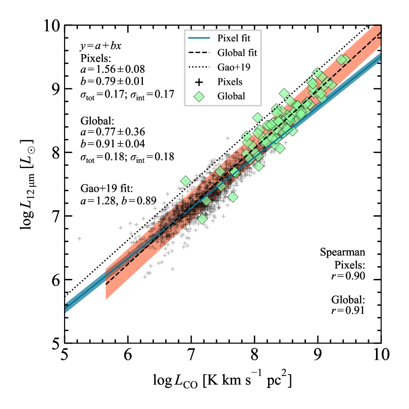
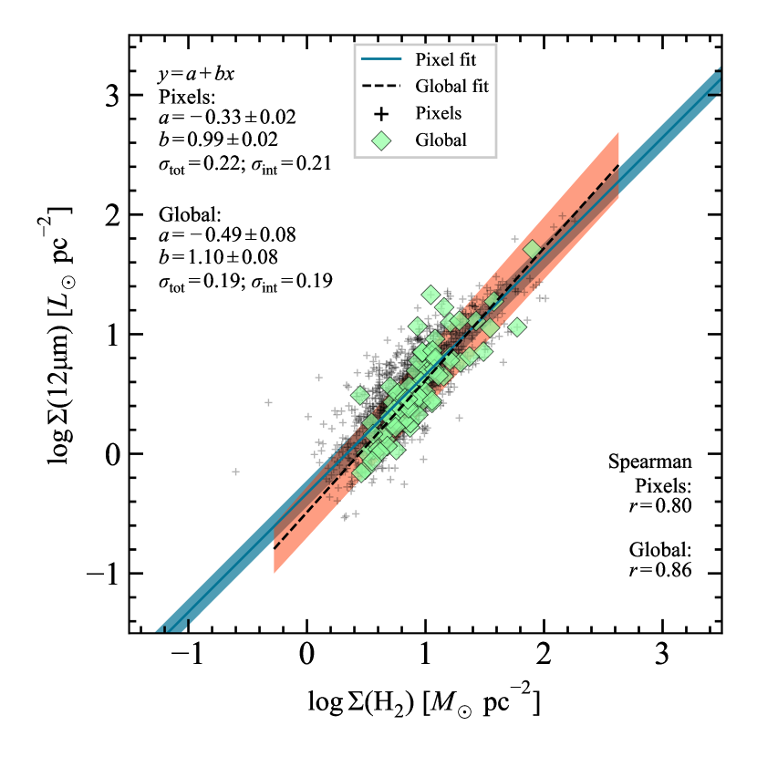
Figure 9: Same as Figure 5 but with the x and y axes interchanged.

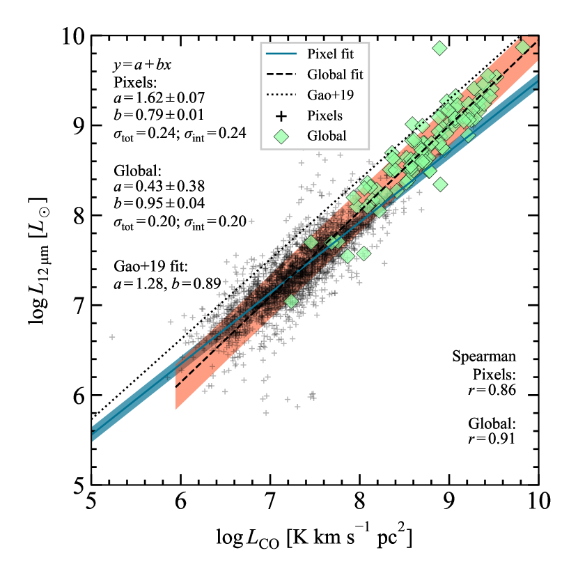
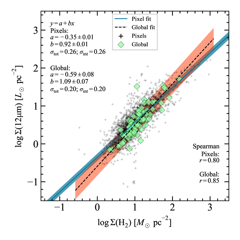
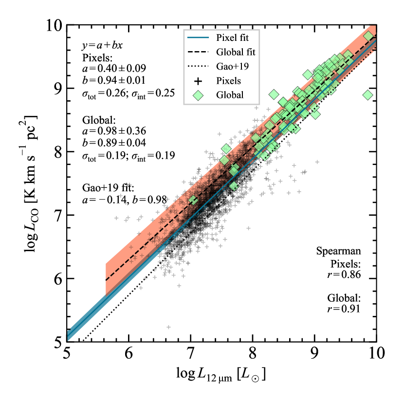
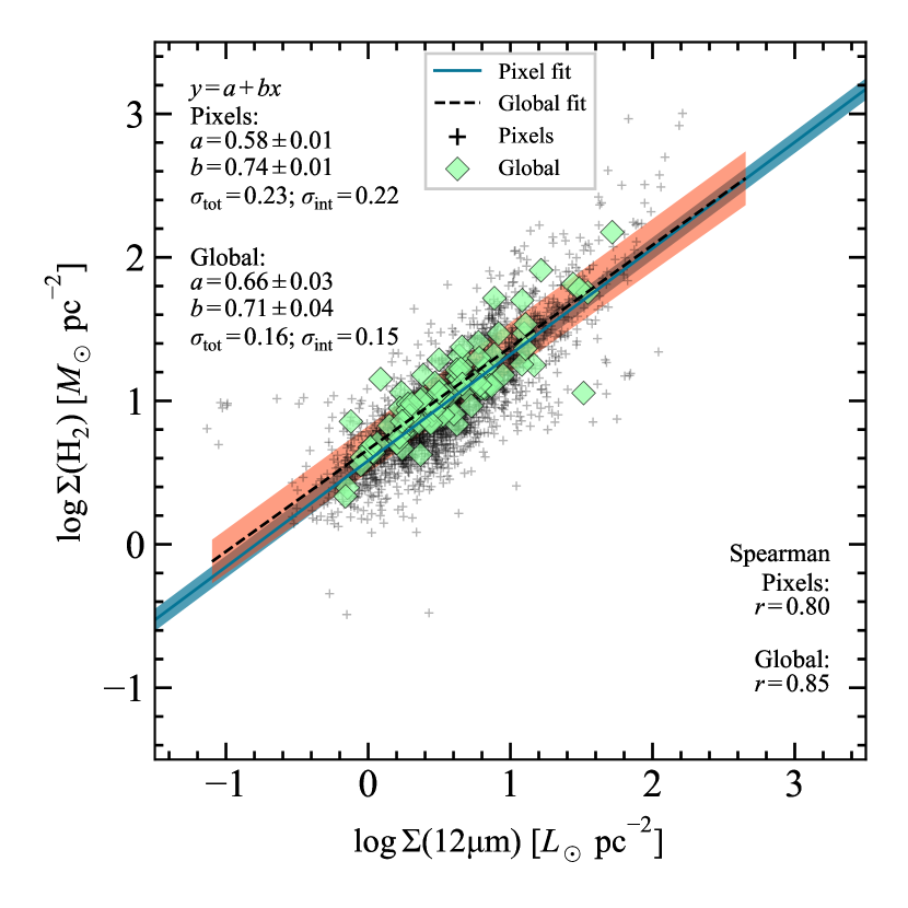
Figure 10: Same as Figure 5 except H₂ surface densities were calculated using $\alpha_{\mathrm{CO}}=3.2\>\mathrm{M_{\odot}}\mathrm{(K\>km\>s^{-1}\>pc^{2})^{-1}}$, and non-starforming pixels were included.

Appendix E Multi-parameter fits assuming a constant $\alpha_{\mathrm{CO}}$

Tables 7, 8, and 9 show the multi-parameter fit results H₂ surface densities were computed assuming $\alpha_{\mathrm{CO}}=3.2\>M_{\odot}\mathrm{(K\>km\>s^{-1}\>pc^{2})^{-1}}$.

Table 7: Same as Table 3 but assuming $\alpha_{\mathrm{CO}}=3.2\>\mathrm{M_{\odot}}\mathrm{(K\>km\>s^{-1}\>pc^{2})^{-1}}$.

					$\theta_{i}$ for pixel properties		$\theta_{i}$ for global properties
RMS error	$n_{\mathrm{gal}}$	$n_{\mathrm{pix}}$	$\sigma_{\mathrm{int}}$	Zero-point ($\theta_{0}$)	$\log\Sigma(\mathrm{12\>\mu m})$	$(12+\log\mathrm{O/H})$	$\log\Sigma_{\mathrm{FUV}}$	$\log\Sigma_{\mathrm{NUV}}$	$A(\mathrm{H\alpha})$
$0.18$	$58$	$1126$	$0.16$	$0.56\pm 0.01$	$0.73\pm 0.01$	–	–	–	–
$0.16$	$30$	$573$	$0.14$	$2.76\pm 0.08$	$0.85\pm 0.01$	–	$-0.21\pm 0.01$	–	–
$0.14$	$27$	$552$	$0.14$	$3.8\pm 0.1$	$0.95\pm 0.01$	–	–	$-0.30\pm 0.01$	$-0.15\pm 0.01$
$0.14$	$27$	$552$	$0.14$	$3.2\pm 0.6$	$0.94\pm 0.01$	$0.06\pm 0.07$	–	$-0.30\pm 0.01$	$-0.15\pm 0.01$

Table 8: Same as Table 4 but assuming $\alpha_{\mathrm{CO}}=3.2\>\mathrm{M_{\odot}}\mathrm{(K\>km\>s^{-1}\>pc^{2})^{-1}}$.

					$\theta_{i}$ for pixel properties	$\theta_{i}$ for global properties
RMS error	$n_{\mathrm{gal}}$	$n_{\mathrm{pix}}$	$\sigma_{\mathrm{int}}$	Zero-point ($\theta_{0}$)	$\log\Sigma(\mathrm{12\>\mu m})$	$\log\Sigma_{\mathrm{FUV}}$	$\log\Sigma_{\mathrm{NUV}}$	$A(\mathrm{H\alpha})$
$0.18$	$58$	$1126$	$0.16$	$0.56\pm 0.01$	$0.73\pm 0.01$	–	–	–
$0.16$	$30$	$573$	$0.14$	$2.76\pm 0.07$	$0.85\pm 0.01$	$-0.21\pm 0.01$	–	–
$0.14$	$27$	$552$	$0.14$	$3.8\pm 0.1$	$0.95\pm 0.01$	–	$-0.30\pm 0.01$	$-0.15\pm 0.01$
$0.14$	$27$	$552$	$0.14$	$3.5\pm 0.1$	$0.92\pm 0.01$	$-0.12\pm 0.03$	$-0.16\pm 0.03$	$-0.14\pm 0.01$

Table 9: Same as Table 5 but assuming $\alpha_{\mathrm{CO}}=3.2\>\mathrm{M_{\odot}}\mathrm{(K\>km\>s^{-1}\>pc^{2})^{-1}}$.

					$\theta_{i}$ for pixel properties			$\theta_{i}$ for global properties
RMS error	$n_{\mathrm{gal}}$	$n_{\mathrm{pix}}$	$\sigma_{\mathrm{int}}$	Zero-point ($\theta_{0}$)	$\log\Sigma_{*}$	$(12+\log\mathrm{O/H})$	$\log\Sigma_{\mathrm{SFR}}$	$\log\Sigma_{\mathrm{NUV}}$	$b/a_{\mathrm{disk}}$
$0.21$	$58$	$1126$	$0.20$	$2.07\pm 0.01$	–	–	$0.50\pm 0.01$	–	–
$0.20$	$42$	$942$	$0.18$	$1.92\pm 0.02$	–	–	$0.49\pm 0.01$	–	$0.21\pm 0.02$
$0.17$	$27$	$552$	$0.18$	$0.8\pm 0.1$	$0.26\pm 0.01$	–	$0.30\pm 0.01$	$0.03\pm 0.01$	–
$0.17$	$27$	$552$	$0.18$	$-3.1\pm 0.6$	$0.23\pm 0.01$	$0.47\pm 0.07$	$0.32\pm 0.01$	$0.02\pm 0.01$	–

References

- Alonso-Herrero et al. (2020) Alonso-Herrero A., et al., 2020, A&A, 639, A43
- Bakes & Tielens (1994) Bakes E. L. O., Tielens A. G. G. M., 1994, ApJ, 427, 822
- Baldwin et al. (1981) Baldwin J. A., Phillips M. M., Terlevich R., 1981, PASP, 93, 5
- Barrera-Ballesteros et al. (2016) Barrera-Ballesteros J. K., et al., 2016, MNRAS, 463, 2513
- Barrera-Ballesteros et al. (2020) Barrera-Ballesteros J. K., et al., 2020, MNRAS, 492, 2651
- Bendo et al. (2008) Bendo G. J., et al., 2008, MNRAS, 389, 629
- Bendo et al. (2020) Bendo G. J., Lu N., Zijlstra A., 2020, MNRAS, 496, 1393
- Bertemes et al. (2018) Bertemes C., et al., 2018, MNRAS, 478, 1442
- Bertin & Arnouts (1996) Bertin E., Arnouts S., 1996, A&AS, 117, 393
- Bigiel et al. (2008) Bigiel F., Leroy A., Walter F., Brinks E., de Blok W. J. G., Madore B., Thornley M. D., 2008, AJ, 136, 2846
- Blanton et al. (2017) Blanton M. R., et al., 2017, AJ, 154, 28
- Bolatto et al. (2013) Bolatto A. D., Wolfire M., Leroy A. K., 2013, ARA&A, 51, 207
- Bolatto et al. (2017) Bolatto A. D., et al., 2017, ApJ, 846, 159
- Calzetti et al. (2007) Calzetti D., et al., 2007, ApJ, 666, 870
- Cappellari (2017) Cappellari M., 2017, MNRAS, 466, 798
- Catalán-Torrecilla et al. (2015) Catalán-Torrecilla C., et al., 2015, A&A, 584, A87
- Churchwell et al. (2006) Churchwell E., et al., 2006, ApJ, 649, 759
- Cid Fernandes et al. (2010) Cid Fernandes R., Stasińska G., Schlickmann M. S., Mateus A., Vale Asari N., Schoenell W., Sodré L., 2010, MNRAS, 403, 1036
- Cluver et al. (2017) Cluver M. E., Jarrett T. H., Dale D. A., Smith J. D. T., August T., Brown M. J. I., 2017, ApJ, 850, 68
- Concas & Popesso (2019) Concas A., Popesso P., 2019, MNRAS, 486, L91
- Cortzen et al. (2019) Cortzen I., et al., 2019, MNRAS, 482, 1618
- Denicoló et al. (2002) Denicoló G., Terlevich R., Terlevich E., 2002, MNRAS, 330, 69
- Diamond-Stanic & Rieke (2010) Diamond-Stanic A. M., Rieke G. H., 2010, ApJ, 724, 140
- Donoso et al. (2012) Donoso E., et al., 2012, ApJ, 748, 80
- Draine et al. (2007) Draine B. T., et al., 2007, ApJ, 663, 866
- Elmegreen (1997) Elmegreen B. G., 1997, in Franco J., Terlevich R., Serrano A., eds, Revista Mexicana de Astronomia y Astrofisica Conference Series Vol. 6, Revista Mexicana de Astronomia y Astrofisica Conference Series. p. 165
- Gao & Solomon (2004) Gao Y., Solomon P. M., 2004, ApJ, 606, 271
- Gao et al. (2019) Gao Y., et al., 2019, ApJ, 887, 172
- Genzel et al. (2012) Genzel R., et al., 2012, ApJ, 746, 69
- Genzel et al. (2015) Genzel R., et al., 2015, ApJ, 800, 20
- Gilhuly & Courteau (2018) Gilhuly C., Courteau S., 2018, MNRAS, 477, 845
- Gilhuly et al. (2019) Gilhuly C., Courteau S., Sánchez S. F., 2019, MNRAS, 482, 1427
- Güver & Özel (2009) Güver T., Özel F., 2009, MNRAS, 400, 2050
- Haas et al. (2002) Haas M., Klaas U., Bianchi S., 2002, A&A, 385, L23
- Hao et al. (2011) Hao C.-N., Kennicutt R. C., Johnson B. D., Calzetti D., Dale D. A., Moustakas J., 2011, ApJ, 741, 124
- Husemann et al. (2013) Husemann B., et al., 2013, A&A, 549, A87
- Jarrett et al. (2011) Jarrett T. H., et al., 2011, ApJ, 735, 112
- Jarrett et al. (2013) Jarrett T. H., et al., 2013, AJ, 145, 6
- Jensen et al. (2017) Jensen J. J., et al., 2017, MNRAS, 470, 3071
- Jiang et al. (2015) Jiang X.-J., Wang Z., Gu Q., Wang J., Zhang Z.-Y., 2015, ApJ, 799, 92
- Jones et al. (2015) Jones A. G., et al., 2015, MNRAS, 448, 168
- Kauffmann et al. (2003) Kauffmann G., et al., 2003, MNRAS, 346, 1055
- Kelly (2007) Kelly B. C., 2007, ApJ, 665, 1489
- Kennicutt (1989) Kennicutt Robert C. J., 1989, ApJ, 344, 685
- Kennicutt & Evans (2012) Kennicutt R. C., Evans N. J., 2012, ARA&A, 50, 531
- Kennicutt et al. (2007) Kennicutt Robert C. J., et al., 2007, ApJ, 671, 333
- Kennicutt et al. (2009) Kennicutt Robert C. J., et al., 2009, ApJ, 703, 1672
- Kewley et al. (2001) Kewley L. J., Dopita M. A., Sutherland R. S., Heisler C. A., Trevena J., 2001, ApJ, 556, 121
- Kroupa & Weidner (2003) Kroupa P., Weidner C., 2003, ApJ, 598, 1076
- Krumholz & Thompson (2007) Krumholz M. R., Thompson T. A., 2007, ApJ, 669, 289
- Leroy et al. (2008) Leroy A. K., Walter F., Brinks E., Bigiel F., de Blok W. J. G., Madore B., Thornley M. D., 2008, AJ, 136, 2782
- Leroy et al. (2013) Leroy A. K., et al., 2013, AJ, 146, 19
- Leroy et al. (2019) Leroy A. K., et al., 2019, ApJS, 244, 24
- Li (2020) Li A., 2020, Nature Astronomy, 4, 339
- Li et al. (2020) Li N., Li C., Mo H., Hu J., Zhou S., Du C., 2020, ApJ, 896, 38
- Madau & Dickinson (2014) Madau P., Dickinson M., 2014, ARA&A, 52, 415
- Makarov et al. (2014) Makarov D., Prugniel P., Terekhova N., Courtois H., Vauglin I., 2014, A&A, 570, A13
- Maloney & Black (1988) Maloney P., Black J. H., 1988, ApJ, 325, 389
- Maragkoudakis et al. (2018) Maragkoudakis A., Ivkovich N., Peeters E., Stock D. J., Hemachandra D., Tielens A. G. G. M., 2018, MNRAS, 481, 5370
- McMullin et al. (2007) McMullin J. P., Waters B., Schiebel D., Young W., Golap K., 2007, in Shaw R. A., Hill F., Bell D. J., eds, Astronomical Society of the Pacific Conference Series Vol. 376, Astronomical Data Analysis Software and Systems XVI. p. 127
- Murata et al. (2014) Murata K. L., et al., 2014, ApJ, 786, 15
- Murphy et al. (2011) Murphy E. J., et al., 2011, ApJ, 737, 67
- Pedregosa et al. (2012) Pedregosa F., et al., 2012, arXiv e-prints, p. arXiv:1201.0490
- Peeters et al. (2004) Peeters E., Spoon H. W. W., Tielens A. G. G. M., 2004, ApJ, 613, 986
- Pope et al. (2013) Pope A., et al., 2013, ApJ, 772, 92
- Povich et al. (2007) Povich M. S., et al., 2007, ApJ, 660, 346
- Regan et al. (2006) Regan M. W., et al., 2006, ApJ, 652, 1112
- Roussel et al. (2001) Roussel H., Sauvage M., Vigroux L., Bosma A., 2001, A&A, 372, 427
- Salim et al. (2016) Salim S., et al., 2016, ApJS, 227, 2
- Salim et al. (2018) Salim S., Boquien M., Lee J. C., 2018, ApJ, 859, 11
- Sánchez et al. (2012) Sánchez S. F., et al., 2012, A&A, 538, A8
- Sánchez et al. (2016) Sánchez S. F., et al., 2016, A&A, 594, A36
- Sandstrom et al. (2010) Sandstrom K. M., Bolatto A. D., Draine B. T., Bot C., Stanimirović S., 2010, ApJ, 715, 701
- Sandstrom et al. (2013) Sandstrom K. M., et al., 2013, ApJ, 777, 5
- Schinnerer et al. (2013) Schinnerer E., et al., 2013, ApJ, 779, 42
- Shetty et al. (2013) Shetty R., Kelly B. C., Bigiel F., 2013, MNRAS, 430, 288
- Shi et al. (2009) Shi Y., et al., 2009, in Wang W., Yang Z., Luo Z., Chen Z., eds, Astronomical Society of the Pacific Conference Series Vol. 408, The Starburst-AGN Connection. p. 209
- Shi et al. (2011) Shi Y., Helou G., Yan L., Armus L., Wu Y., Papovich C., Stierwalt S., 2011, ApJ, 733, 87
- Shi et al. (2018) Shi Y., et al., 2018, ApJ, 853, 149
- Shipley et al. (2013) Shipley H. V., Papovich C., Rieke G. H., Dey A., Jannuzi B. T., Moustakas J., Weiner B., 2013, ApJ, 769, 75
- Shipley et al. (2016) Shipley H. V., Papovich C., Rieke G. H., Brown M. J. I., Moustakas J., 2016, ApJ, 818, 60
- Silk (1997) Silk J., 1997, ApJ, 481, 703
- Sun et al. (2018) Sun J., et al., 2018, ApJ, 860, 172
- Tacconi et al. (2018) Tacconi L. J., et al., 2018, ApJ, 853, 179
- Tielens (2008) Tielens A. G. G. M., 2008, ARA&A, 46, 289
- Tommasin et al. (2010) Tommasin S., Spinoglio L., Malkan M. A., Fazio G., 2010, ApJ, 709, 1257
- Walcher et al. (2014) Walcher C. J., et al., 2014, A&A, 569, A1
- Werner et al. (2004) Werner M. W., et al., 2004, ApJS, 154, 1
- Whitcomb et al. (2020) Whitcomb C. M., Sandstrom K., Murphy E. J., Linden S., 2020, arXiv e-prints, p. arXiv:2008.05496
- Wilson (1995) Wilson C. D., 1995, ApJ, 448, L97
- Wright et al. (2010) Wright E. L., et al., 2010, AJ, 140, 1868
- Wu et al. (2005) Wu H., Cao C., Hao C.-N., Liu F.-S., Wang J.-L., Xia X.-Y., Deng Z.-G., Young C. K.-S., 2005, ApJ, 632, L79
- Xie & Ho (2019) Xie Y., Ho L. C., 2019, ApJ, 884, 136
- Yesuf & Ho (2019) Yesuf H. M., Ho L. C., 2019, ApJ, 884, 177
- Yesuf & Ho (2020) Yesuf H. M., Ho L. C., 2020, arXiv e-prints, p. arXiv:2007.14004