Conditional Gradient Methods for Convex Optimization
with General Affine and Nonlinear Constraints
††thanks:
This research was partially supported by the ONR grant N00014-20-1-2089 and NSF grant CCF 1909298.
Abstract
Conditional gradient methods have attracted much attention in both machine learning and optimization communities recently. These simple methods can guarantee the generation of sparse solutions. In addition, without the computation of full gradients, they can handle huge-scale problems sometimes even with an exponentially increasing number of decision variables. This paper aims to significantly expand the application areas of these methods by presenting new conditional gradient methods for solving convex optimization problems with general affine and nonlinear constraints. More specifically, we first present a new constraint extrapolated condition gradient (CoexCG) method that can achieve an iteration complexity for both smooth and structured nonsmooth function constrained convex optimization. We further develop novel variants of CoexCG, namely constraint extrapolated and dual regularized conditional gradient (CoexDurCG) methods, that can achieve similar iteration complexity to CoexCG but allow adaptive selection for algorithmic parameters. We illustrate the effectiveness of these methods for solving an important class of radiation therapy treatment planning problems arising from healthcare industry. To the best of our knowledge, all the algorithmic schemes and their complexity results are new in the area of projection-free methods.
1 Introduction
In this paper, we focus on the development of conditional gradient type methods for solving the following convex optimization problem:
| (1.1) | ||||
| s.t. | ||||
Here is a compact convex set, and , , are proper lower semicontinuous convex functions, denotes a linear mapping, and is a given vector in . We assume that is relatively simple in the sense that one can minimize a linear function over easily. Throughout this paper we assume that an optimal solution of problem (1.1) exists. For notational convenience, we often denote .
The conditional gradient method, initially developed by Frank and Wolfe in 1956 [8], is one of the earliest first-order methods for convex optimization. It has been widely used for solving problems with relatively simple convex sets, i.e., when the constraints and do not appear in problem (1.1). Each iteration of this method computes the gradient of at the current search point , and then solves the subproblem to update the solution. In comparison with most other first-order methods, it does not require the projection over , which in many cases could be computationally more expensive than to minimize a linear function over (e.g.. when is a spectrahedron given by ). These simple methods can also guarantee the generation of sparse solutions, e.g., when is a simplex or spectrahedron. In addition, without the computation of full gradients, they can handle huge-scale problems sometimes even with an exponentially increasing number of decision variables.
Much recent research effort has been devoted to the complexity analysis of conditional gradient methods over simple convex set . It is well-known that if is a smooth convex function, then this algorithm can find an -solution (i.e., a point s.t. ) in at most iterations (see [16, 17, 20, 9, 14]). In fact, such a complexity result has been established for the conditional gradient method under a stronger termination criterion called Wolfe Gap, based on the first-order optimality condition [16, 17, 20, 9, 14]. As shown in [16, 20, 12], this iteration complexity bound is tight for smooth convex optimization. In addition, if is a nonsmooth function with a saddle point structure, one can not achieve an iteration complexity better than [20], in terms of the number of times to solve the linear optimization subproblem. One possible way to improve the complexity bounds is to use the conditional gradient sliding methods developed in [23] to reduce the number of gradient evaluations. Many other variants of conditional gradient methods have also been proposed in the literature (see, e.g.,[1, 2, 3, 6, 9, 15, 14, 16, 17, 24, 35, 36, 18, 5, 11]) and Chapter 7 of [21] for an overview of these methods).
It should be noted, however, that none of the existing conditional gradient methods can be used to efficiently solve the more general function constrained convex optimization problem in (1.1). With these function constraints ( and ), linear optimization over the feasible region of problem (1.1) could become much more difficult. As an example, if is the aforementioned spectrahedron and does not exist, the linear optimization problem over the feasible region becomes a general semidefinite programming problem. Adding nonlinear function constraints usually makes the subproblem even harder. In fact, our study has been directly motivated by a convex optimization problem with nonlinear function constraints arising from radiation therapy treatment planning (see [7, 25, 34, 10, 26, 27, 28] and Section 4 for more details). The objective function of this problem, representing the quality of the treatment plan, is smooth and convex. Besides a simplex constraint, it consists of two types of nonlinear function constraints, namely the group sparsity constraint to reduce radiation exposure for the patients, and the risk averse constraints to avoid overdose (resp., underdose) to healthy (resp., tumor) structures. This problem is highly challenging because the dimension of the decision variables can increase exponentially with respect to the size of data, which prevents the computation of full gradients as required by most existing optimization methods dealing with function constraints.
This paper aims to fill in the aforementioned gap in the literature by presenting a new class of conditional gradient methods for solving problem (1.1). Our main contributions are briefly summarized as follows. Firstly, inspired by the constraint-extrapolation (ConEx) method for function constrained convex optimization in [4], we develop a novel constraint-extrapolated conditional gradient (CoexCG) method for solving problem (1.1). While both methods are single-loop primal-dual type methods for solving convex optimization problems with function constraints, CoexCG only requires us to minimize a linear function, rather than to perform projection, over . In the basic setting when both and are smooth convex functions with Lipschitz continuous gradients, we show that the total number of iterations performed by CoexCG before finding a -solution of problem (1.1), i.e., a point s.t. and , can be bounded by . Here .
Secondly, we consider more general function constrained optimization problems where either the objective function or some constraint functions are possibly nondifferentiable, but contains certain saddle point structure. We extend the CoexCG method for solving these problems in combination with the well-known Nesterov’s smoothing scheme [32]. In general, even equipped with such smoothing technique, nonsmooth optimization is more difficult than smooth optimization, and its associated iteration complexity is worse than that for smooth ones by orders of magnitude. However, we show that a similar complexity bound can be achieved by CoexCG for solving these nonsmooth function constrained optimization problems. This seemly surprising result can be attributed to an inherent acceleration scheme in CoexCG that can reduce the impact of the Lipschitz constants induced by the smoothing scheme.
Thirdly, one possible shortcoming of CoexCG exists in that it requires the total number of iterations fixed a priori before we run the algorithm in order to achieve the best rate of convergence. Therefore it is inconvenient to implement this algorithm when such an iteration limit is not available. In order to address this issue, we propose a constraint-extrapolated and dual-regularized conditional gradient (CoexDurCG) method by adding a diminishing regularization term for the dual updates. This modification allows us to design a novel adaptive stepsize policy which does not require given in advance. Moreover, we show that the complexity of CoexDurCG is still in the same order of magnitude as CoexCG with a slightly larger constant factor. We also extend CoexDurCG for solving the aforementioned structured nonsmooth problems, and demonstrate that it is not necessary to explicitly define the smooth approximation problem. We note that this technique of adding a diminishing regularization term can be applied for solving problems with either unbounded primal feasible region (e.g., stochastic subgradient descent [30] and stochastic accelerated gradient descent [19]), or unbounded dual feasible region (e.g., ConEx [4]), for which one often requires the number of iterations fixed in advance.
Finally, we apply the developed algorithms for solving the radiation therapy treatment planning problem on both randomly generated instances and a real data set. We show that CoexDurCG performs comparably to CoexCG in terms of solution quality and computation time. We demonstrate that the incorporation of function constraints helps us not only to find feasible treatment plans satisfying clinical criteria, but also generate alternative treatment plans that can possibly reduce radiation exposure time for the patients.
To the best of our knowledge, all the algorithmic schemes as well as their complexity results are new in the area of projection-free methods for convex optimization.
This paper is organized as follows. Section 2 is devoted to the CoexCG method. We first present the CoexCG method for smooth function constrained convex optimization in Subsection 2.1 and extend it for solving structured nonsmooth function constrained convex optimization in Subsection 2.2. We then discuss the CoexDurCG method in Section 3, including its basic version for smooth function constrained convex optimization in Subsection 3.1 and its extended version for directly solving structured nonsmooth function constrained convex optimization problems in Subsection 3.2. We apply these methods for radiation therapy treatment planning in Section 4, and conclude the paper with a brief summary in Section 5.
2 Constraint-extrapolated conditional gradient method
In this section, we present a basic version of the constraint-extrapolated conditional gradient method for solving convex optimization problem (1.1). Subsection 2.1 focuses on the case when and are smooth convex functions, while subsection 2.2 extends our discussion to the situation where and are not necessarily differentiable.
2.1 Smooth functions
Throughout this subsection, we assume that and are differential and their gradients are Lipschitz continuous s.t.
| (2.1) | ||||
| (2.2) |
Here denotes an arbitrary norm which is not necessarily associated with the inner product ( is the conjugate norm of ). For notational convenience, we denote
We need to use the Lipschitz continuity of the constraint function when developing conditional gradient methods for function constrained problems. Clearly, under the boundedness assumption of , the constraint functions are Lipschitz continuous with constant , i.e.,
| (2.3) |
In particular, letting be an optimal solution of problem (1.1), we have where denotes the diameter of given by
| (2.4) |
Note that a different way to bound on will be discussed for certain structured nonsmooth problems in Subsection 2.2. For the sake of notational convenience, we also denote
| (2.5) |
Since we can only perform linear optimization over the feasible region , one natural way to solve problem (1.1) is to consider its saddle point reformulation
| (2.6) |
Throughout the paper, we assume that the standard Slater condition holds for problem (1.1) so that a pair of optimal dual solutions of problem (2.6) exists.
In [32], Nesterov proposed a novel smoothing scheme to solve a general bilinear saddle point problem when the term does not exist in (2.6). More specifically, he suggested to apply an accelerated gradient method to solve a smooth approximation for this bilinear saddle point problem. Using this idea, in [20] (see also Chapter 7 of [21]), Lan presented a smoothing conditional gradient method by appling the conditional gradient algorithm for a properly smoothed version of the objective function of (2.6). However, this scheme is not applicable for our setting due to the following reasons. Firstly, the smoothing conditional gradient method only solves bilinear saddle point problems with linear coupling terms given by and cannot deal with the nonlinear coupling term . Secondly, even for the bilinear saddle point problems, the smoothing conditional gradient method in [21, 20] requires the feasible set of to be bounded, which does not hold for problem (2.6).
Our development has been inspired the constraint extrapolation (ConEx) method recently introduced by Boob, Deng and Lan [4] for solving problem (2.6). ConEx is an accelerated primal-dual type method which updates both the primal variable and dual variables in each iteration. In comparison with some previously developed accelerated primal-dual methods for solving saddle point problems with nonlinear coupling terms [29, 13], one distinctive feature of ConEx is that it defines the acceleration (or momentum) step by extrapolating the linear approximation of the nonlinear function . As a consequence, it can deal with unbounded feasible regions for the dual variable (or ) and thus solve the function (or affine) constrained convex optimization problems. However, each iteration of the ConEx method requires the projection onto the feasible region , and hence is not applicable to our problem setting.
In order to address the above issues for solving problem (1.1) (or (2.6)), we present a novel constraint-extrapolated conditional gradient (CoexCG) method, which incorporates some basic ideas of the ConEx method into the conditional gradient method. As shown in Algorithm 1, the CoexCG method first performs in (2.9) an extrapolation step for the affine constraint . Then in (2.10) it performs an extrapolation step based on the linear approximation of the constraint function given by
| (2.7) | |||
| (2.8) |
Utilizing the extrapolated constraint values and , it then updates the dual variables and associated with the affine constraint and the nonlinear constraints in (2.11) and (2.12), respectively. With these updated dual variables and linear approximation and , it solves a linear optimization problem over to update the primal variable in (2.13). Finally, the output solution is computed as a convex combination of and in (2.14).
| (2.9) | ||||
| (2.10) | ||||
| (2.11) | ||||
| (2.12) | ||||
| (2.13) | ||||
| (2.14) |
Similar to the game interpretation developed in [22, 21] for Nesterov’s accelerated gradient method [31], the CoexCG method can be viewed as an iterative game performed by the primal and dual players to achieve an equilibrium of (2.6). The extrapolation steps in (2.9)-(2.10) are used to predict the possible action (or its consequences) of the primal player in each iteration. Based on the prediction , the dual player updates the decision (resp., ) in order to maximize the profit (resp., ), but not to move too far away from the previous decision (resp., ) by using the regularization (resp., ). After observing the dual player’s decisions , the primal player first determines in a greedy manner by minimizing the cost , and then takes a correction step in (2.14) so that its decision is not dramatically different from the previous decision . Similar to Nesterov’s method as interpreted in [22, 21], CoexCG employs an intelligent dual player who predicts the other player’s decision before taking actions. However, the primal updates in (2.13) and (2.14) for CoexCG are different from those in [22, 21] since no projection is allowed, even though the spirit of not moving too far away from the previous decision remains the same. An interesting observation to us is that, due to the lack of the projection for the primal player, the incorporation of the extrapolation (or prediction) steps of the dual player appears to be important to guarantee the convergence of the algorithm (see the discussion after Proposition 3 for more details).
It is interesting to build some connections between the CoexCG method and the ConEx method in [4]. In particular, by replacing the relations in (2.13) and (2.14) with
then we essentially obtain the ConEx method. Comparing these relations, we observe that the CoexCG method differs from the ConEx method in the following few aspects. Firstly, in CoexCG is computed by solving a linear optimization problem, while the one in the ConEx method is computed by using a projection. The use of linear optimization enables the CoexCG method to generate sparse solutions in feasible sets with a huge large number of extreme points (see Section 4). Secondly, the linear approximation models and in the ConEx method is built on the search point , while the one in the CoexCG method is built on , or equivalently, the convex combination of all previous search points , . Using and in CoexCG instead of and as in ConEx also seems to be critical to guarantee the convergence of the CoexCG algorithm.
We need to add a few more remarks about the CoexCG method. Firstly, by (2.11) and (2.12), we can define and equivalently as
It is also worth noting that we can generalize the CoexCG method to deal with conic inequality constraint , by simply replacing the constraint in (2.12) with . Here is a given closed convex cone and denotes its the dual cone.
Secondly, in addition to the primal output solution in (2.14), we can also define the dual output solutions and as
| (2.15) | ||||
| (2.16) |
Different from , these dual variables and do not participate in the updating of any other search points. However, both of them will be used intensively in the convergence analysis of the CoexCG method.
Thirdly, even though we do not need to select the parameter when defining as in the ConEx method, we do need to specify the stepsize parameter to update the dual variables and . We also need to determine the parameters and , respectively, to define the extrapolation steps and the output solution . We will discuss the selection of these algorithmic parameters after establishing some general convergence properties of the CoexCG method.
Our goal in the remaining part of this subsection is to establish the convergence of the CoexCG method. Let , and be defined in (2.14), (2.15), and (2.16). Throughout this section, we denote and , and define the gap function as
| (2.17) |
We start by stating some well-known technical results that have been used in the convergence analysis of many first-order methods. The first result, often referred to “three-point lemma” (see, e.g., Lemma 3.1 of [21]), characterizes the optimality conditions of (2.11) and (2.12).
The following result helps us to take telescoping sums (see Lemma 3.17 of [21]).
Lemma 2.
Let , be given and denote
| (2.20) |
If satisfies then we have
We now establish an important recursion of the CoexCG method.
Proposition 3.
Proof. It follows from the smoothness of and (e.g., Lemma 3.2 of [21]) and the definition of in (2.14) that
Using the above two relations in the definition of in (2.17), we have for any ,
Moreover, by the definition of in (2.14) and the convexity of and , we have
Combining the above two relations, we obtain
| (2.21) |
Multiplying both sides of (2.18) and (2.19) by and summing them up with the above inequality, we have
| (2.22) |
Now observe that by the definition of in (2.9) and the fact that , we have
| (2.23) |
where the first inequality follows from Young’s inequality and the last one follows from the definition of in (2.4). In addition, by the definition of in (2.10), we have
| (2.24) |
where the last inequality follows from
| (2.25) |
The result then follows by plugging relations (2.23) and (2.24) into (2.22).
We add some comments about the importance of the extrapolation steps in the proposed CoexCG method. Without these steps (i.e., in (2.9) and (2.10)), probably we can not even guarantee the convergence of the CoexCG algorithm. As we can see from the proof of Proposition 3, if , it is not clear how to take care of the inner product terms and . The error caused by these terms may accumulate.
We are now ready to establish the main convergence properties for the CoexCG method.
Theorem 4.
Proof. It follows from Lemma 2 and Proposition 3 that
which, in view of (2.26), then implies that
where the last relation follows from Young’s inequality and a result similar to (2.25). The result in (2.27) then immediately follows from the above inequality.
Note that by the definition of in (2.17), and the facts that and , we have . Using this observation and fixing in (2.27), we obtain (2.28). Now let us denote
| (2.30) | ||||
| (2.31) | ||||
| (2.32) |
Note that by the optimality condition of (2.6), we have
In addition, using the fact that and , we have
Combining the previous two observations, we conclude that
| (2.33) |
The previous conclusion, together with (2.27) and the facts that
| (2.34) | ||||
| (2.35) | ||||
| (2.36) |
then imply that
Below we provide a specific selection of the algorithmic parameters , and and establish the associated rate of convergence for the CoexCG method.
Corollary 5.
If the number of iterations is fixed a priori, and
| (2.37) |
then we have
| (2.38) | ||||
| (2.39) | ||||
| (2.40) |
Proof. By (2.20) and the definition of in (2.37), we have and . We can easily see from these identities and (2.37) that the conditions in (2.26) hold. It is also easy to verify that
Using these relations in (2.27), (2.28) and (2.29), we conclude that
and
A few remarks about the results obtained in Theorem 4 and Corollary 5 are in place. Firstly, in view of (2.38), the gap function converges to with the rate of convergence given by . This bound has been shown to be not improvable in [20] for general saddle point problems in terms of the number of calls to linear optimization oracles (see also Chapter 7 of [21]), even though such a lower complexity bound cannot be directly applied to our setting since we are dealing with a specific saddle point problem with unbounded dual variables. Secondly, in view of (2.39) and (2.40), the number of iterations required by the CoexCG method to find a -solution of problem (1.1), i.e., a point s.t. and , is bounded by . Thirdly, it is interesting to observe that in both (2.39) and (2.40), the Lipschitz constants and do not impact too much the rate of convergence of the CoexCG method, since both of them appear only in the non-dominant terms. We will explore further this property of the CoexCG method in order to solve problems with certain nonsmooth objective and constraint functions. Finally, it is worth noting that in the parameter setting (2.37), we need to fix the total number of iterations in advance. This is not desirable for the implementation of the CoexCG method, especially for the situation when one has finished the scheduled iterations, but then realizes that a more accurate solution is needed. In this case, one has to completely restart the CoexCG method with a different parameter setting that depends on the modified iteration limit. We will discuss how to address this issue in Section 3.
2.2 Structured nonsmooth functions
In this subsection, we still consider problem (1.1), but the objective function and constraint functions are not necessarily differentiable. More specifically, we assume that and are given in the following form:
| (2.41) | ||||
where and are closed convex sets, and and are simple convex functions. Many nonsmooth functions can be represented in this form (see [32]). In this paper, we assume that and are possibly strongly convex w.r.t. the given norms in the respective spaces, i.e..
| (2.42) | |||
| (2.43) |
for some . If (resp., ), then (resp., ) must be differentiable with Lipschitz continuous gradients. Therefore, our nonsmooth formulation in (2.41) allows either the objective and/or some constraint functions to be smooth.
Our goal in this subsection is to generalize the CoexCG method to solve these structured nonsmooth convex optimization problems. In fact, we show that that the number of CoexCG iterations required to solve these problems is in the same order of magnitude as if and ’s are smooth convex functions.
Since and are possibly not differentiable, we cannot directly apply the CoexCG algorithm to solve problem (1.1). However, as pointed out by Nesterov [32], these nonsmooth functions can be closely approximated by smooth convex ones. Let us first consider the objective function . Assume that is a given strongly convex function with modulus w.r.t. a given norm in , i.e.,
Let us denote , and
| (2.44) |
and define
| (2.45) |
for some . Then, we can show that is differentiable and its gradients satisfy (see [32])
| (2.46) |
In addition, we have
| (2.47) |
In our algorithmic scheme, we will set whenever is strongly convex, i.e., .
Similarly, let us assume that are strongly convex with modulus w.r.t. a given norm in , . Also let us denote , and
| (2.48) |
and define
| (2.49) |
for some . We can show that for all ,
| (2.50) | |||
| (2.51) |
In our algorithmic scheme, we will set whenever is strongly convex, i.e., . For notational convenience, we denote
| (2.52) |
Different from the objective function, we need to show that the gradient of the is bounded. Note that the boundedness of the gradients for smooth constraint functions (with and hence ) follows from the boundedness of (see Section 2.1). For those nonsmooth constraint functions (with ), we need to assume that ’s are compact. For a given , let be the optimal solution of (2.49). Then
| (2.53) |
For notational convenience, we also denote
| (2.54) |
Observe that the Lipschitz constants defined in (2.53) do not depend on the smoothing parameters , . This fact will be important for us to derive the complexity bound of the CoexCG method for solving convex optimization problems with nonsmooth function constraints.
Instead of solving the original problem (1.1), we suggest to apply the CoexCG method to the smooth approximation problem
| (2.55) | ||||
| s.t. | ||||
More specifically, we replace the linear approximation functions and used in (2.10) and (2.13) by and , respectively. However, we will establish the convergence of this method in terms of the solution of the original problem in (1.1) rather than the approximation problem in (2.55). Our convergence analysis below exploits the smoothness of (resp., ), the closeness between and (resp., and ), and also importantly, the fact that underestimates for all .
Theorem 6.
Consider the CoexCG method applied to the smooth approximation problem (2.55). Assume that the number of iterations is fixed a priori, and that the parameters and are set to (2.37) with replaced by in (2.54). Then we have
| (2.56) | ||||
| (2.57) |
where is a triple of optimal solutions for problem (2.6), and are defined in (2.46) and (2.52), respectively, and , and are defined in (2.4), (2.44) and (2.48), respectively.
Proof. Denote . In view of Corollary 5, we have
| (2.58) |
for any . Using the relations in (2.47) and (2.51), and the fact that , we can see that
| (2.59) |
By letting , and , we have
which, in view of (2.58), then implies (2.56). Now let be defined in (2.32). By (2.33), (2.58) and (2.59), we have
where the last inequality follows from the bounds in (2.34) and (2.35), and the facts that and
We now specify the selection of the smoothing parameters , . We consider only the most challenging case when the objective and all constraint functions are nonsmooth and establish the rate of convergence of the aforementioned CoexCG method for nonsmooth convex optimization.
Corollary 7.
Proof. It follows from (2.46), (2.52) and (2.60) that and that
Also notice that and that
Using these identities and the assumptions in (2.56) and (2.57), we have
We add a few remarks about the results obtained in Theorem 6 and Corollary 7. Firstly, in view of Corollary 7, even if and are nonsmooth functions, the number of CoexCG iterations required to find an -solution of problem (1.1) is still bounded by . Therefore, by utilizing the structural information of and , the CoexCG can solve this type of nonsmooth problem efficiently as if they are smooth functions. Secondly, if either the objective function or some constraint functions are smooth, we can set the corresponding smoothing parameter to be zero and obtain slightly improved complexity bounds than those in Corollary 7. Thirdly, similar to the CoexCG method applied for solving problem (1.1) with smooth objective and constraint functions, we need to fix the number of iterations in advance when specifying the algorithmic parameters and smoothing parameters. We will address this issue in the next section.
3 Constraint-extrapolated and dual-regularized conditional gradient method
One critical shortcoming associated with the basic version of the CoexCG method is that we need to fix the number of iterations a priori. Our goal in this section is to develop a variant of CoexCG which does not have this requirement. We consider the case when and are smooth and structured nonsmooth functions, respectively, in Subsections 3.1 and 3.2.
3.1 Smooth functions
In order to remove the assumption of fixing a priori, we suggest to modify the dual projection steps (2.11) and (2.12) in the CoexCG method. More specifically, we add an additional regularization term with diminishing weights into these steps. This variant of CoexCG is formally described in Algorithm 2.
Clearly, we can write and in (3.1) and (3.2) equivalently as
Similar to the CoexCG method, it is also possible to generalize CoexDurCG for solving problems with conic inequality constraints. The following result, whose proof can be found in Lemma 3.5 of [21], characterizes the optimality conditions for (3.1) and (3.2).
We now establish an important recursion about the CoexDurCG method, which can be viewed as a counterpart of Proposition 3 for the CoexCG method.
Proposition 9.
Proof. Multiplying both sides of (3.3) and (3.4) by and summing them up with the inequality in (2.21), we have
| (3.5) |
The result then follows by plugging relations (2.23) and (2.24) into (3.5).
We are now ready to establish the main convergence properties of the CoexDurCG method.
Theorem 10.
Proof. It follows from Lemma 2 and Proposition 9 that
which, in view of (3.6), then implies that
where the last relation follows from Young’s inequality and a result similar to (2.25). The result in (2.27) then immediately follows from the above inequality. We can show (3.8) and (3.9) similarly to (2.28) and (2.29), and hence the details are skipped.
Corollary 11 below shows how to specify the algorithmic parameters, including the regularization weight , for the CoexDurCG method. In particular, the selection of was inspired by the one used in (2.37), and was chosen so that the last relation in (3.6) is satisfied.
Corollary 11.
If the algorithmic parameters , , and of the CoexDurCG method are set to
| (3.10) |
with for , then we have, ,
| (3.11) |
In addition, we have
| (3.12) |
and
| (3.13) |
where denotes a triple of optimal solutions for problem (2.6).
Proof. From the definition of in (3.10), we have and . Hence the first two conditions in (3.6) hold. In addition, it follows from these identities and (3.10) that and
and hence that the last relation in (3.6) also holds. Observe that by (3.10),
| (3.14) | ||||
| (3.15) | ||||
| (3.16) |
Using these relations in (3.7), we have
The bounds in (3.12) and (3.13) can be shown similarly and the details are skipped.
In view of the results obtained in Corollary 11, the rate of convergence of CoexDurCG matches that of CoexCG. Moreover, the cost of each iteration of the CoexDurCG is the same as that of CoexCG.
3.2 Structured Nonsmooth Functions
In this subsection, we consider problem (1.1) with structured nonsmooth functions and given in (2.41). One possible way to solve this nonsmooth problem is to apply the CoexDurCG method for the smooth approximation problem (2.55). However, this approach still requires us to fix the number of iterations when choosing smoothing parameters , .
Our goal in this subsection is to generalize the CoexDurCG method to solve this structured nonsmooth problem directly. Rather than applying this algorithm to problem (2.55), we modify the smoothing parameters , , at each iteration. More specifically, we assume that
| (3.17) |
and define a sequence of smoothing functions and , , according to (2.45) and (2.49), respectively. For simplicity, we denote
Also let us define the Lipschitz constants
It can be seen from (3.17) that
| (3.18) |
Indeed, it suffices to show the second relation in (3.18). By definition, we have
where the inequality follows from the definition of in (2.44) and the assumption in (3.17). Similarly, we have
| (3.19) |
Note that in our algorithmic scheme, we can set , , if the corresponding objective or constraint functions are smooth (i.e., ).
We now describe the more general CoexDurCG method for solving structured nonsmooth problems.
In Algorithm 3 we do not explicitly use the smooth approximation problem (2.55). Instead, we incorporate in (3.20) and (3.21) the adaptive linear approximation functions and for the objective and constraints, respectively. The convergence analysis of this algorithm relies on the adaptive primal-dual gap function:
| (3.22) |
as demonstrated in the following result.
Proposition 12.
Proof. Similar to (3.5), we can show that
| (3.23) |
Moreover, by the definition of in (3.20), we have
| (3.24) |
where the last inequality follows from
| (3.25) |
Here, the first inequality follows from Young’s inequality, the second inequality follows from the cauchy-schwarz inequality, the definition of in (2.4) and the bound of in (2.53), the third inequality follows by the relation between and in (3.19) and the simple fact that , and the last inequality follows from the Lipschitz continuity of and the bound in (2.53). In addition, it follows from (3.18) and (3.19) that for any ,
| (3.26) |
The result follows by combining (3.23), (3.24), (3.26) and the bound in (2.23).
Theorem 13.
Proof. It follows from Lemma 2, Proposition 12 and (3.6) that
where the last relation follows from Young’s inequality and a result similar to (3.25). The result in (3.27) then immediately follows from the above inequality and the observation that due to (2.59). We can show (3.28) and (3.29) similarly to (2.56) and (2.57), and hence the details are skipped.
Corollary 14 below shows how to specify the smoothing parameter in (3.17) and other parameters for the CoexDurCG method in Algorithm 3. We focus on the most challenging case when the objective function and all the constraint functions are nonsmooth (i.e., , ). Slightly improved rate of convergence can be obtained by setting for those component functions with .
Corollary 14.
Proof. From the definition of in (3.10), we have and . Similarly to Corollary 11, we can check that condition (3.6), and the bounds in (3.14)-(3.16) hold. In addition, it follows from the definition of in (3.30) that
Using these relations in (3.27), we have
which implies (3.31) after simplification. (3.32) and (3.33) can be shown similarly and the details are skipped.
Comparing the results in Corollary 14 with those in Corollary 7, we can see that the rate of convergence of CoexDurCG is about the same as that of CoexCG for nonsmooth optimization. However, it is more convenient to implement CoexDurCG since it does not require us to fix the number of iterations a priori.
4 Numerical Experiments
In this section, we apply the proposed algorithms to the intensity modulated radiation therapy (IMRT) problem briefly discussed in Section 1.
4.1 Problem Formulation
In IMRT, the patient will be irradiated by a linear accelerator (linac) from several angles and in each angle the device uses different apertures. In traditional IMRT, we select and fix 5-9 angles and then design and optimize the apertures and their corresponding intensity. Following [34], we would like to integrate the angle selection into direct aperture optimization in order to use a small number of angles and apertures in the final treatment plan.
To model the IMRT treatment planning, we discretize each structure of the patient into small cubic volume elements called voxels, . There are a finite number of angles, denoted by , around the patient. A beam in each angle, , is decomposed into a rectangular grid of beamlets. A beamlet is effective if it is not blocked by either the left, , and right, , leaves. An aperture is then defined as the collection of effective beamlets. The relative motion of the leaves controls the set of effective beamlets and thus the shape of the aperture. The estimated dose received by voxel from beamlet at unit intensity is denoted by in Gy. The dose absorbed by a given voxel is the summation of the dose from each individual beamlet.
Let be the set of allowed apertures determined by the position of the left and right leaves in beam angle . Suppose that the rectangular grid in each angle has rows and columns, and the leaves move along each row independently. Then the number of possible apertures in each angle amounts to . We use , comprised of binary decision variables , to describe the shape of aperture . In particular, if beamlet is effective, i.e., falling within the left and right leaves of row , otherwise . In addition to selecting angles and apertures, we also need to determine the influence rate for aperture , which will be used to determine the dose intensity and the amount of radiation time from aperture . The dose absorbed by voxel is computed by , based on the dose-influence matrix , the aperture shape , and the aperture influence rate . We measure the treatment quality by via voxel-based quadratic penalty, where denotes , and and are pre-specified lower and upper dose thresholds for voxel .
We also need to consider a few important function constraints. Firstly, in order to obtain a sparse solution with a small number of angles, we add the following group sparsity constraint for some properly chosen . Intuitively, this constraint will encourage the selection of apertures in those angles that have already contained some nonzero elements of , . Secondly, we need to meet a few critical clinical criteria to avoid underdose (resp., overdose) for tumor (resp., healthy) structures. These criteria are usually specified as value at risk (VaR) constraints. For example, in the prostate benchmark dataset, the clinical criterion of “PTV56:V56” means that the percentage of voxels in structure PTV56 that receive at least 56 Gy dose should be at least . Similarly, the criterion of “PTV68: V74.8” implies that the percentage of voxels in structure PTV68 that receive more than 74.8 Gy dose should be at most . One possible way to satisfy these criteria is to tune the weights () in . However, it would be time consuming to tune these weights to satisfy all the prescribed clinical criteria. Therefore, we suggest to incorporate a few critical criteria as problem constraints explicitly.
Instead of using VaR, we will use its convex approximation, commonly referred to as Conditional Value at Risk (CVaR) in the constraints [33]. Recall the following definitions of VaR and CVaR
| Upper tail: | |||
| Lower tail: |
The upper (resp., lower) tail CVaR will be used to enforce the underdose (resp., overdose) clinical criteria. For example, letting and denote structures PTV68 and PTV 56, and and be the number of voxels in these structures, we can approximately formulate the criterion of “PTV68: V74.8” as for some . Separately, the criterion of “PTV56:V56” will be approximated by or equivalently for some . Putting the above discussions together and denoting , we obtain the following problem formulation.
| (4.1a) | ||||
| s.t. | (4.1b) | |||
| (4.1c) | ||||
| (4.1d) | ||||
| (4.1e) | ||||
| (4.1f) | ||||
| (4.1g) | ||||
| (4.1h) | ||||
where OD and UD denote the set of overdose and underdose clinical criteria, respectively. Clearly, the objective function is convex and smooth. Constraints in (4.1c), (4.1d) and (4.1e) are structured nonsmooth function constraints corresponding to the function constraints in (1.1), while (4.1f)-(4.1g) and (4.1h), respectively, define a simplex constraint on and a box constraint on , with their Catesian product corresponding to the convex set in (1.1). The bounds and in constraints (4.1h) can be obtained from the corresponding clinical criteria. For example, the criterion of “PTV68:V68” implies that value at risk . By the definition of CVaR, the optimal equals to the value at risk, hence we set . In a similar way, we set in view of the criterion of “PTV68: V74.8”.
We can apply the CoexCG and CoexDurCG methods described in Subsections 2.2 and 3.2, respectively, to solve problem (4.1a)-(4.1h). Since the number of the potential apertures (i.e., the dimension of ) increases exponentially w.r.t. , we cannot compute the full gradient of the objective and constraint functions w.r.t. . Instead, we will perform gradient computation and linear optimization simultaneously. Let us focus on the CoexCG method for illustration. Denote the constraints (4.1c)-(4.1e) as , , and let the corresponding smooth approximation be defined by (2.49) (using entropy distances for smoothing). For a given search point and dual variable , let us denote and . Clearly, in view of (2.13), will be updated to a properly chosen extreme point of the simplex constraint in (4.1f)-(4.1g). In order to determine this extreme point, we need to find the aperture with the smallest coefficient in the linear objective of (2.13) given by:
This can be achieved by using the following constructive approach. For any row of the rectangular grid in angle , we find the column indices and , respectively, for the left and right leaves, that give the most negative value of . Repeating this process row by row, we construct the aperture with the smallest value of in angle . We construct one aperture similar to this for each angle, and then choose the one with the most negative value of among all the angles. Therefore, to solve the linear optimization suproblem (i.e., to find the aperture with the smallest coefficient) only requires arithmetic operations, even though the dimension of the problem (i.e., the total number of apertures) is given by .
4.2 Comparison of CoexCG and CoexDurCG on randomly generated instances
Due to the privacy issue, publicly available IMRT datasets for real patients are very limited. To test the performance of our proposed algorithms we first randomly generate some problem instances as follows. Let be a cube with length . Viewing as the human body, we then arbitrarily choose two (or more) cuboids as healthy organs, and randomly choose 2 cubes inside as the target tumor tissues. For a given accuracy , we discretize all these structures into small cubes with length to define a voxel. Around the cube , we generate a circle with radius on the plane , and define every two degrees as one angle for radiation therapy. In each angle, we consider the aperture as a square in , and also discretize it with small squares with length , resulting in a grid with size . After that, we randomly generate beamlets with coordinate for each angle . As for the matrix (recording the dose received by voxel from each beamlet), we first check if the voxel is radiated by the beamlet since each beamlet is a line perpendicular to the aperture plane. If so, the dose received by the voxel from this beamlet will be set to , where is the distance between the voxel and the aperture plane; otherwise, the dose is . By choosing different accuracy , we can create instances with different sizes in terms of the number of voxels and potential apertures. Table 1 shows five different test instances generated with . We set and for the first three instances (Ins. 1, Ins. 2 and Ins. 3), and the last two instances (Ins. 4 and Ins. 5), respectively. Note that we consider 2 underdose and 1 overdose constraints and their corresponding r.h.s. and are shown in the last column of Table 1. We set the for tumor tissue and for healthy organ in (4.1a). In addition, we set for the group sparsity constraint in (4.1e).
We implement in Matlab the CoexCG and CoexDurCG algorithms for structured nonsmooth problems, and report the computational results in Table 2. Here we use , and , respectively, to denote the output solution, the objective value and constraint violations. The CPU times are in seconds on a Macbook Pro with 2.6 GHz 6-Core Intel Core i7 processor. As shown in Table 2, both CoexCG and CoexDurCG exhibit comparable performance in terms of objective value, constraint violation and CPU time for different iteration limit . However, unlike the CoexDurCG algorithm, we need to rerun CoexCG for all the experiments whenever changes.
| Index | of voxels | of apertures | |
| Ins. 1 | 4096 | 460800 | [30,40,200] [0.05,0.05,0.05] |
| Ins. 2 | 4096 | 460800 | [40,50,100] [0.01,0.01,0.05] |
| Ins. 3 | 4096 | 460800 | [50,60,80] [0.01,0.01,0.01] |
| Ins. 4 | 262144 | 7372800 | [40,50,100] [0.01,0.01,0.05] |
| Ins. 5 | 262144 | 7372800 | [50,60,80] [0.01,0.01,0.01] |
| Index | N | CoexCG | CoexDurCG | ||||
| CPU(s) | CPU(s) | ||||||
| Ins. 1 | 1 | 46.8723 | 1.7237e+03 | ||||
| 100 | 0.0683 | 0.4234 | 34 | 0.0616 | 0.3705 | 33 | |
| 1000 | 0.0197 | 0.0319 | 323 | 0.0210 | 0.0219 | 327 | |
| Ins. 2 | 1 | 46.8723 | 1.7237e+03 | ||||
| 100 | 0.0568 | 0.4424 | 33 | 0.0583 | 0.5002 | 34 | |
| 1000 | 0.0224 | 0.0426 | 327 | 0.0232 | 0.0334 | 339 | |
| Ins. 3 | 1 | 46.8723 | 1.7237e+03 | ||||
| 100 | 0.0625 | 13.7567 | 33 | 0.0604 | 7.3929 | 33 | |
| 1000 | 0.0227 | 0.0514 | 332 | 0.0226 | 0.0193 | 332 | |
| Ins. 4 | 1 | 47.7099 | 8.7850e+03 | ||||
| 100 | 0.4643 | 163.3043 | 1645 | 0.4643 | 163.3043 | 1645 | |
| 1000 | 0.0398 | 12.1765 | 17254 | 0.0398 | 12.1765 | 17356 | |
| Ins. 5 | 1 | 47.7099 | 8.7850e+03 | ||||
| 100 | 0.4866 | 253.9389 | 1644 | 0.4581 | 206.9143 | 1637 | |
| 1000 | 0.0406 | 39.2051 | 17146 | 0.0417 | 38.6486 | 17607 | |
In order to test our CoexCG and CoexDurCG algorithms, we still want to compare them with some existing algorithm for constrained convex problems, such as ConEx algorithm [boob2019stochastic]. Since the most existing algorithms will require the computation of full gradient and hence get in stuck when dealing with this very high dimensional problems, we generated a very small dimensional problem (dimension of decision variable is 80000) with similar problem formulation for comparison. From Table 3, we see the ConEx algorithm still requires the computation of full gradient, and hence has a total around 630 second computational time of the matrix for every component. And also we can see the ConEx algorithm finally converges to a almost feasible solution with a bit higher objective function value comparing to the solutions of CoexCG and CoexDurCG algorithms. We also implemented the ConEx algorithm to the Instances 1-5, but the algorithm gets in stuck in the first iteration and keeps running forever.
| N | Alg | CPU(s) | ||
| 2 | ConEx | 0.482 | 32.156 | 632.902 |
| CoexCG | 0.495 | 64.738 | 0.143 | |
| CoexDurCG | 0.495 | 64.738 | 0.156 | |
| 10 | ConEx | 0.311 | 6.137 | 633.948 |
| CoexCG | 0.033 | 9.381 | 0.692 | |
| CoexDurCG | 0.074 | 8.913 | 0.654 | |
| 100 | ConEx | 0.279 | 0.193 | 642.456 |
| CoexCG | 0.010 | 6.165 | 6.501 | |
| CoexDurCG | 0.015 | 6.384 | 6.535 | |
| 1000 | ConEx | 0.301 | 7.392e-04 | 725.477 |
| CoexCG | 0.010 | 6.626 | 63.958 | |
| CoexDurCG | 0.022 | 6.361 | 66.661 |
4.3 Results for real dataset
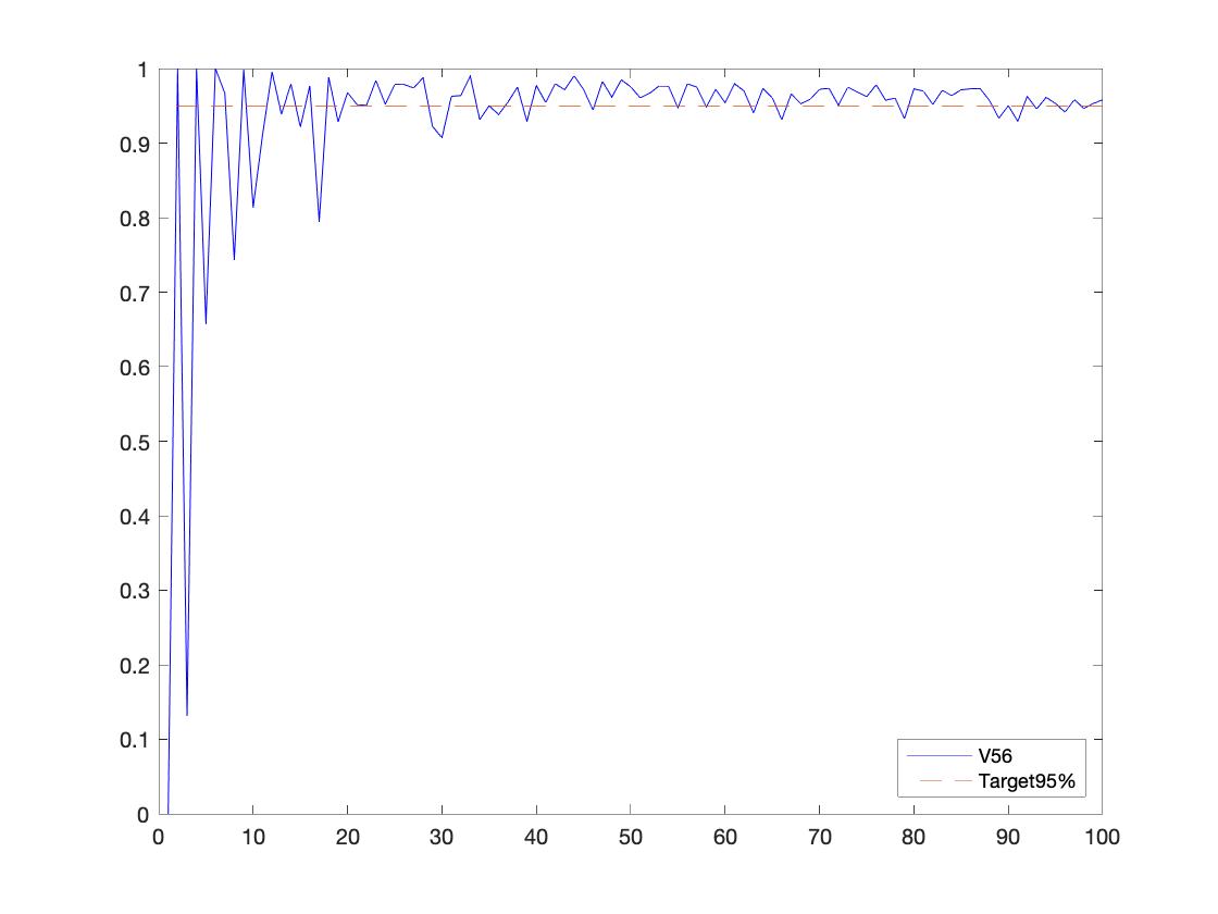
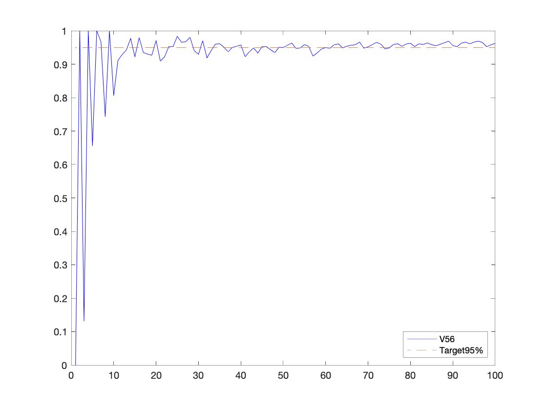
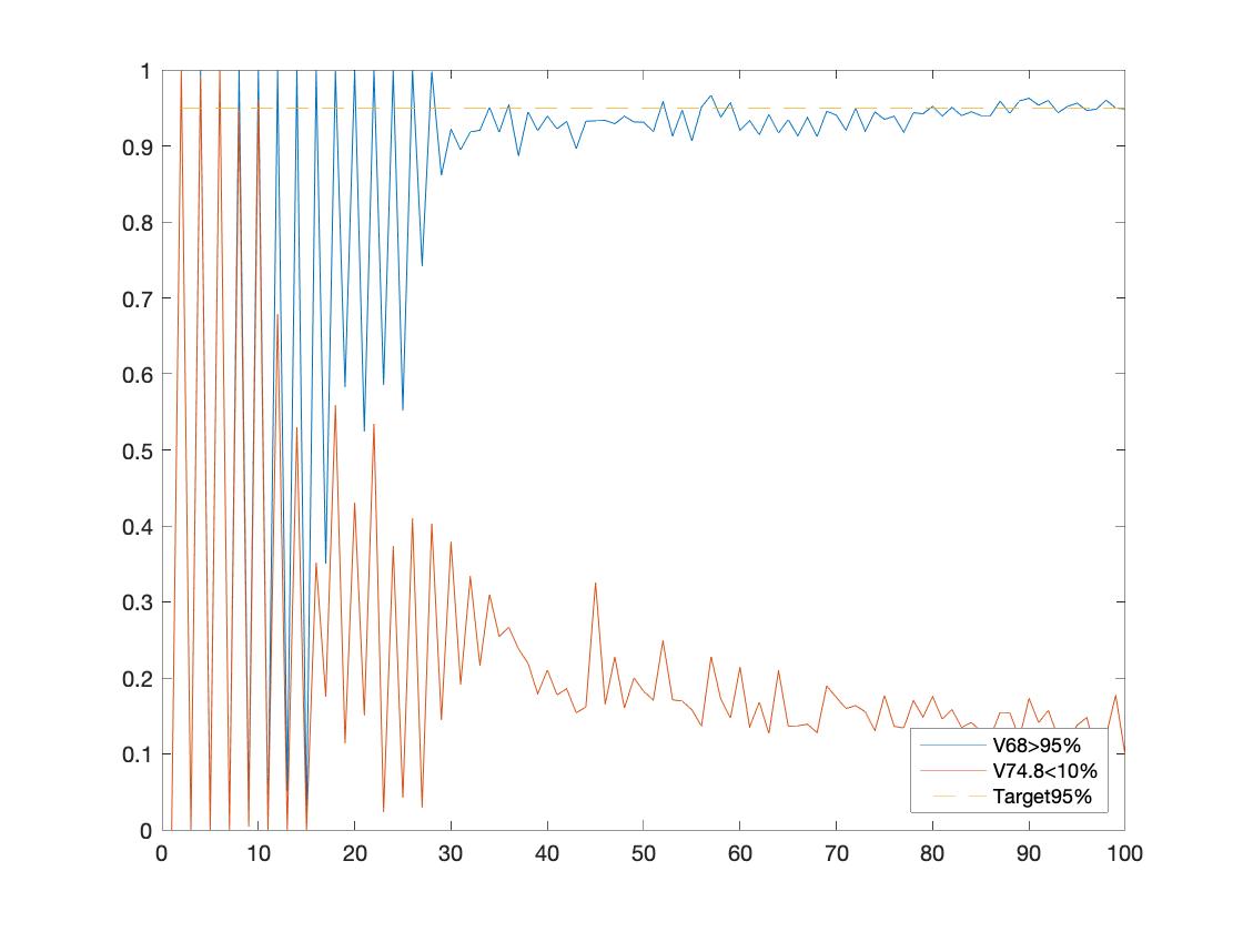
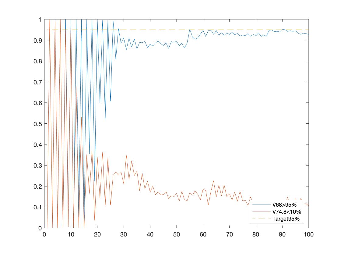
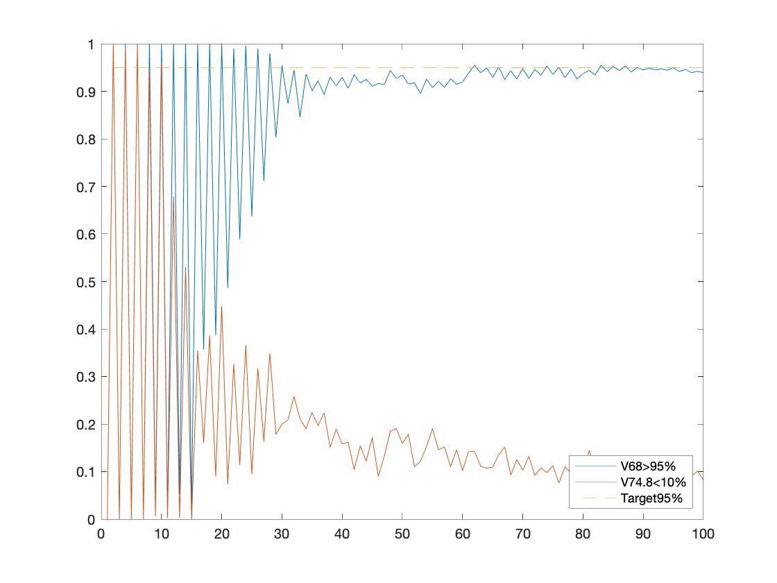
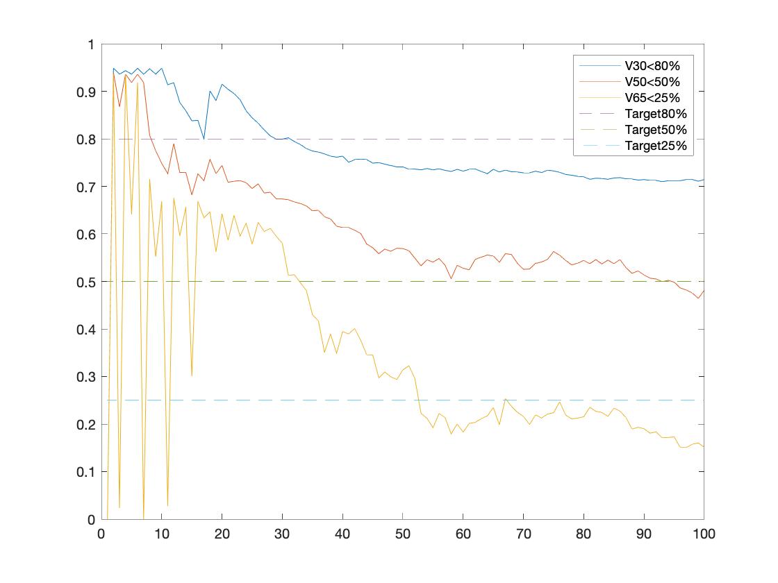
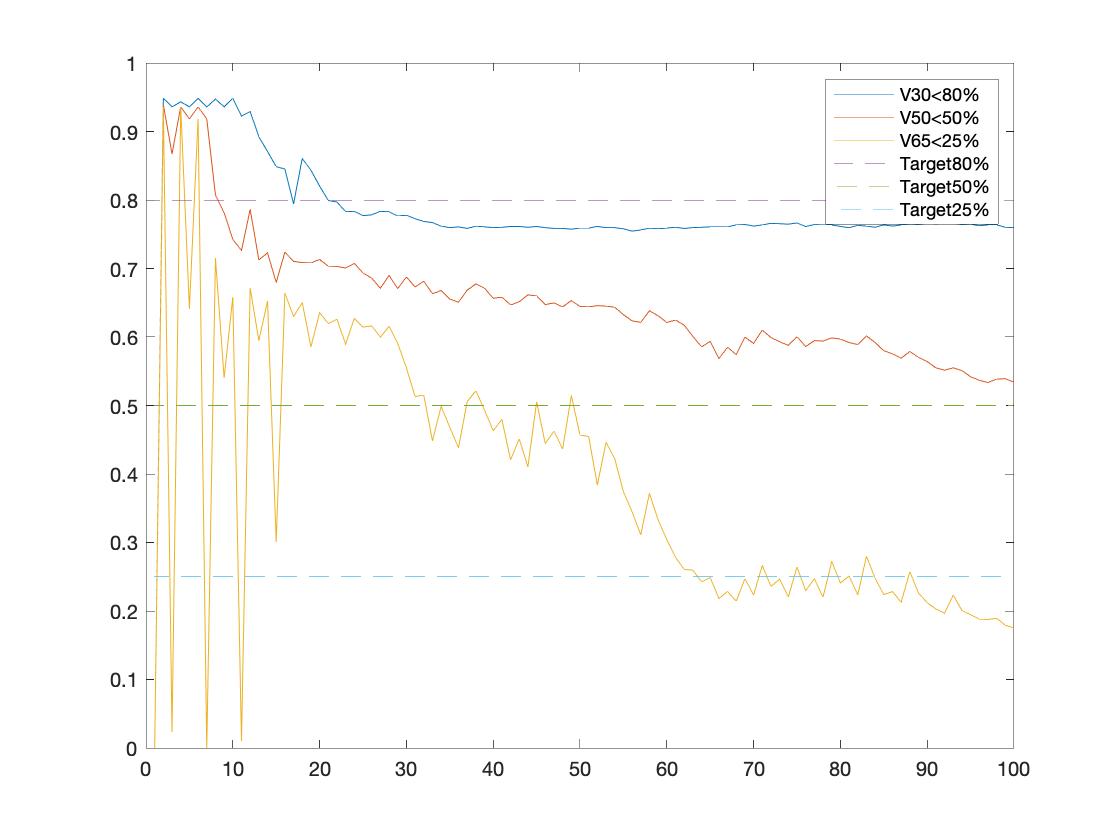
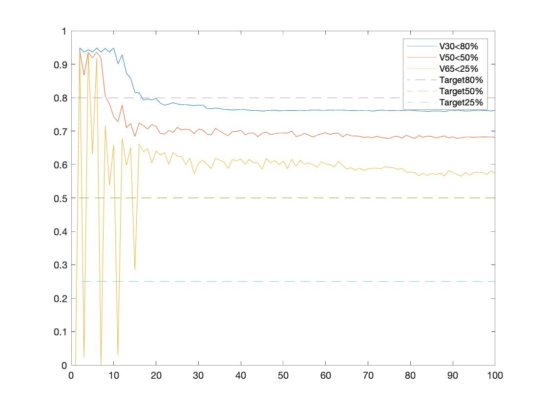
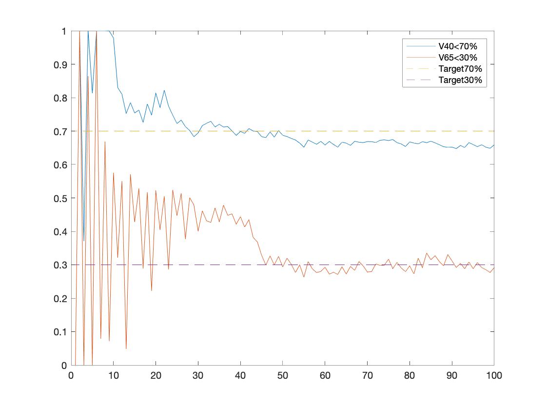
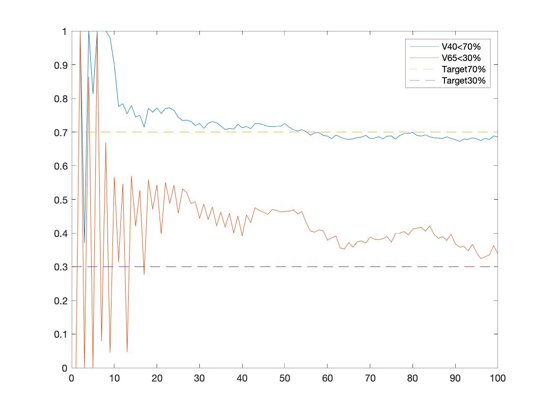
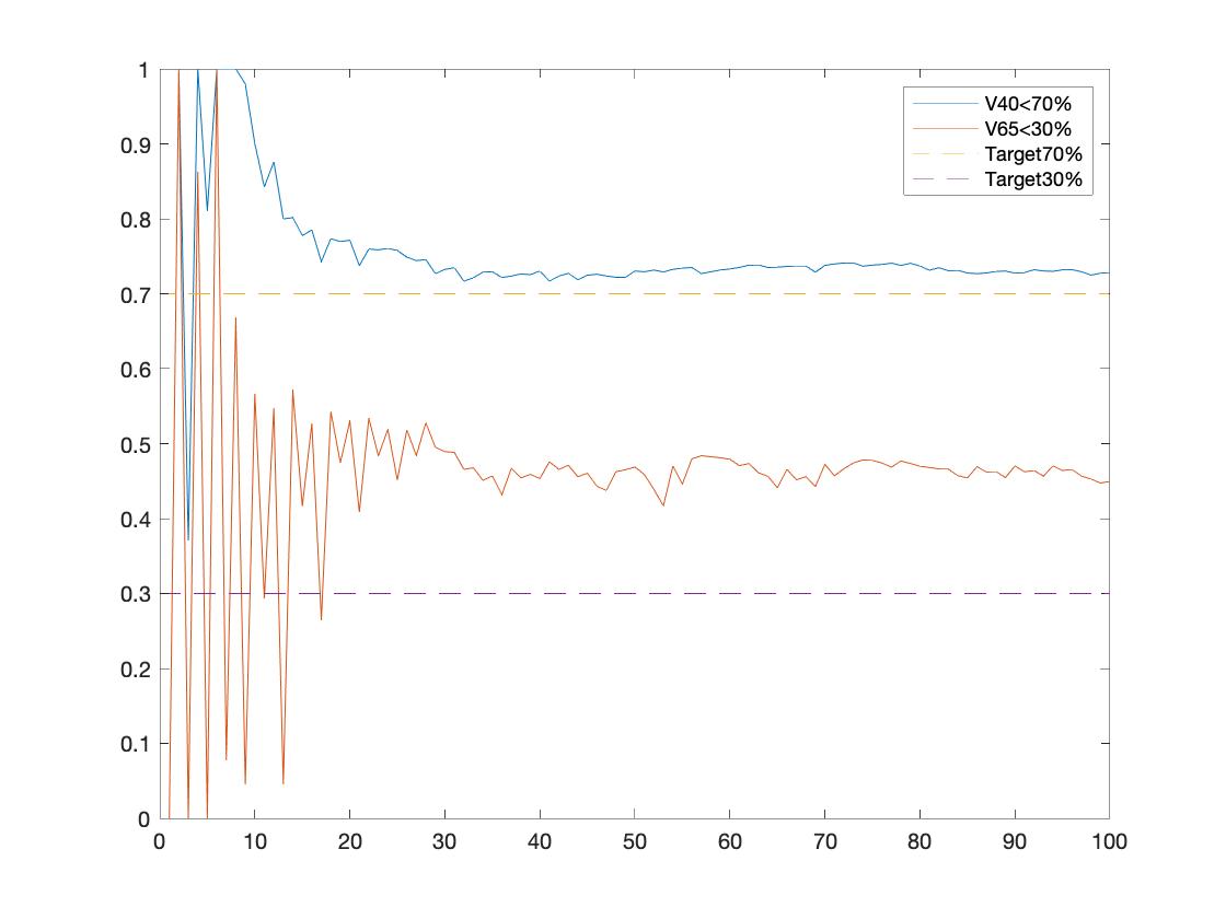
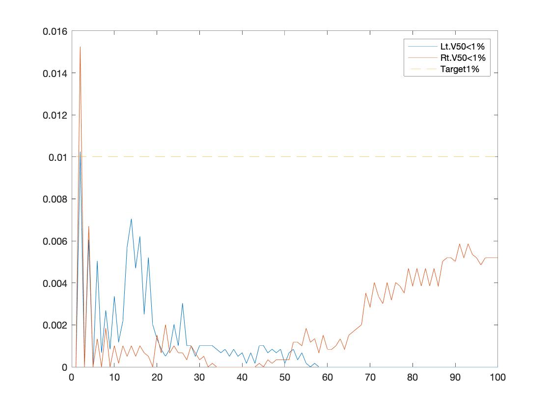
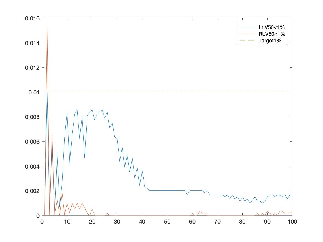
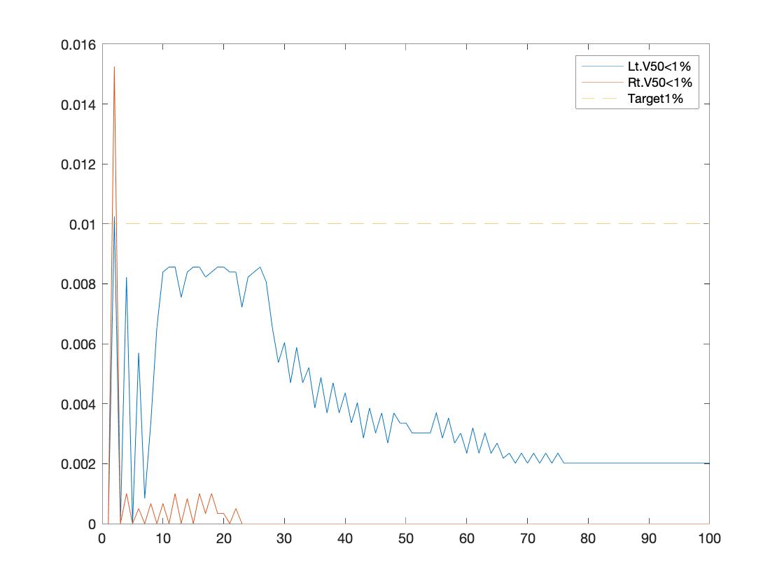
In this subsection, we apply CoexDurCG to the real dataset for a patient with prostate cancer (https://github.com/cerr/CERR/wiki), and evaluate the generated solution from the clinical point of view. Dose volume histogram (DVH), a histogram relating radiation dose to tissue volume in radiation therapy planning, is commonly used as a plan evaluation tool to compare doses received by different structures under different plans [7, 25]. In this prostate dataset, there are totally 10 DVH criteria as follows, PTV56: V56; PTV68: V68, V74.8; Rectum: V30, V50, V65; Bladder: V40, V65; Left femoral head: V50; Right femoral head: V50. For this dataset, we have voxels, angles and over potential apertures in each angle.
Since a smaller number of angles results in shorter treatment duration, we study the quality of the treatment plan generated when enforcing the group sparsity requirement with different in (4.1e). In order to balance the scale of the constraint violation, we normalized all the constraints (4.1c)-(4.1e) by dividing both sides of the inequalities by the right hand side or . The total number of apertures in a typical treatment plan for this dataset would not be greater than . Thus, we set the iteration limit to 100 since the CoexDurCG algorithm generates at most one new aperture in each iteration.
Table 4 shows the number of apertures/angles, objective value and constraints violation for different solutions given different values of . Figure 1 plots the DVH performance of the generated treatment plans by presenting how the percentage of voxels in each organ changes over different iterations. If , the constraint (4.1e) is redundant and we obtain a solution with the smallest function value and zero constraints violation, but with the largest number of angles as shown in Table 4. In addition, the plots in the first column (i.e., parts (a), (d), (g), (j) and (m)) of Figure 1 show that the generated plan satisfies all the DVH criteria. Comparing the first two rows in Table 4, we see that the solutions remain the same when . By keeping decreasing , we can obtain solutions with fewer angles. Plots in the second column of Figure 1 shows that most DVH criteria are still satisfied even if the number of angles in the solution reduces from 39 to 8. Moreover, the number of angles can be decreased to 3 if we are willing to sacrifice certain DVH criteria as we can see from the plots in the third column of Figure 1.
| of apertures | of angles | Obj. Val. | Con. Vio. | |
| 1 | 96 | 39 | 0.0902 | 0 |
| 0.1 | 96 | 39 | 0.0902 | 0 |
| 0.005 | 96 | 8 | 0.1027 | 0.098 |
| 0.0005 | 97 | 3 | 0.1357 | 0.0589 |

5 Concluding Remarks
In this paper, we propose new constraint-extrapolated conditional gradient (CoexCG) methods for solving general convex optimization problems with function constraints. These methods require only linear optimization rather than projection over the convex set . We establish the iteration complexity for CoexCG and show that the same complexity still holds even if the objective or constraint functions are nonsmooth with certain structures. We further present novel dual regularized algorithms that do not require us to fix the number of iterations a priori and show that they can attain complexity bounds similar to CoexCG. Effectiveness of these methods are demonstrated for solving a challenging function constrained convex optimization problems arising from IMRT treatment planning.
It seems to be possible to use some ideas from the conditional gradient sliding methods [23] to improve the number of gradient computation of and , as well as the operator evaluation of . However, the conditional gradient sliding type methods would require us to compute and store the full gradient information. For the IMRT treatment planning problem, it is impossible to compute the full gradient since its dimension increases exponentially with the size of aperture. Nevertheless, incorporating the idea of conditional gradient sliding for solving problems with function constraints will be an interesting topic for future research.
References
- [1] S. Ahipasaoglu and M. Todd. A modified frank-wolfe algorithm for computing minimum-area enclosing ellipsoidal cylinders: Theory and algorithms. Computational Geometry, 46:494–519, 2013.
- [2] F. Bach, S. Lacoste-Julien, and G. Obozinski. On the equivalence between herding and conditional gradient algorithms. In the 29th International Conference on Machine Learning, 2012.
- [3] A. Beck and M. Teboulle. A conditional gradient method with linear rate of convergence for solving convex linear systems. Math. Methods Oper. Res., 59:235–247, 2004.
- [4] D. Boob, Q. Deng, and G. Lan. Stochastic first-order methods for convex and nonconvex function constrained optimization. arXiv, 2019. 1908.02734.
- [5] G. Braun, S. Pokutta, and D. Zink. Lazifying conditional gradient algorithms. In ICML, pages 566–575, 2017.
- [6] K. L. Clarkson. Coresets, sparse greedy approximation, and the frank-wolfe algorithm. ACM Trans. Algorithms, 6(4):63:1–63:30, Sept. 2010.
- [7] R. Drzymala, R. Mohan, L. Brewster, J. Chu, M. Goitein, W. Harms, and M. Urie. Dose-volume histograms. International Journal of Radiation Oncology* Biology* Physics, 21(1):71–78, 1991.
- [8] M. Frank and P. Wolfe. An algorithm for quadratic programming. Naval Research Logistics Quarterly, 3:95–110, 1956.
- [9] R. M. Freund and P. Grigas. New Analysis and Results for the Frank-Wolfe Method. ArXiv e-prints, July 2013.
- [10] M. Goitein. Radiation oncology: a physicist’s-eye view. Springer Science & Business Media, 2007.
- [11] M. L. Gonçalves and J. G. Melo. A newton conditional gradient method for constrained nonlinear systems. Journal of Computational and Applied Mathematics, 311:473–483, 2017.
- [12] C. Guzmán and A. Nemirovski. On lower complexity bounds for large-scale smooth convex optimization. Journal of Complexity, 31(1):1–14, 2015.
- [13] E. Y. Hamedani and N. S. Aybat. A primal-dual algorithm for general convex-concave saddle point problems. arXiv preprint arXiv:1803.01401, 2018.
- [14] Z. Harchaoui, A. Juditsky, and A. S. Nemirovski. Conditional gradient algorithms for machine learning. NIPS OPT workshop, 2012.
- [15] E. Hazan. Sparse approximate solutions to semidefinite programs. In E. Laber, C. Bornstein, L. Nogueira, and L. Faria, editors, LATIN 2008: Theoretical Informatics, volume 4957 of Lecture Notes in Computer Science, pages 306–316. Springer Berlin Heidelberg, 2008.
- [16] M. Jaggi. Revisiting frank-wolfe: Projection-free sparse convex optimization. In the 30th International Conference on Machine Learning, 2013.
- [17] M. Jaggi and M. Sulovský. A simple algorithm for nuclear norm regularized problems. In the 27th International Conference on Machine Learning, 2010.
- [18] B. Jiang, T. Lin, S. Ma, and S. Zhang. Structured nonconvex and nonsmooth optimization: algorithms and iteration complexity analysis. Computational Optimization and Applications, 72(1):115–157, 2019.
- [19] G. Lan. An optimal method for stochastic composite optimization. Mathematical Programming, 133(1):365–397, 2012.
- [20] G. Lan. The complexity of large-scale convex programming under a linear optimization oracle. arXiv preprint arXiv:1309.5550, 2013.
- [21] G. Lan. First-order and Stochastic Optimization Methods for Machine Learning. Springer Nature, Switzerland AG, 2020.
- [22] G. Lan and Y. Zhou. An optimal randomized incremental gradient method. Mathematical programming.
- [23] G. Lan and Y. Zhou. Conditional gradient sliding for convex optimization. Technical report, Technical Report, 2014.
- [24] R. Luss and M. Teboulle. Conditional gradient algorithms for rank one matrix approximations with a sparsity constraint. SIAM Review, 55:65–98, 2013.
- [25] P. Mayles, A. Nahum, and J.-C. Rosenwald. Handbook of radiotherapy physics: theory and practice. CRC Press, 2007.
- [26] C. Men, X. Gu, D. Choi, A. Majumdar, Z. Zheng, K. Mueller, and S. B. Jiang. Gpu-based ultrafast imrt plan optimization. Physics in Medicine & Biology, 54(21):6565, 2009.
- [27] C. Men, H. E. Romeijn, X. Jia, and S. B. Jiang. Ultrafast treatment plan optimization for volumetric modulated arc therapy (vmat). Medical physics, 37(11):5787–5791, 2010.
- [28] C. Men, H. E. Romeijn, Z. C. Taşkın, and J. F. Dempsey. An exact approach to direct aperture optimization in imrt treatment planning. Physics in Medicine & Biology, 52(24):7333, 2007.
- [29] A. S. Nemirovski. Prox-method with rate of convergence for variational inequalities with lipschitz continuous monotone operators and smooth convex-concave saddle point problems. SIAM Journal on Optimization, 15:229–251, 2005.
- [30] A. S. Nemirovski, A. Juditsky, G. Lan, and A. Shapiro. Robust stochastic approximation approach to stochastic programming. SIAM Journal on Optimization, 19:1574–1609, 2009.
- [31] Y. E. Nesterov. A method for unconstrained convex minimization problem with the rate of convergence . Doklady AN SSSR, 269:543–547, 1983.
- [32] Y. E. Nesterov. Smooth minimization of nonsmooth functions. Mathematical Programming, 103:127–152, 2005.
- [33] R. Rockafellar and S. Uryasev. Optimization of conditional value-at-risk. The Journal of Risk, 2:21–41, 2000.
- [34] H. E. Romeijn, R. K. Ahuja, J. F. Dempsey, and A. Kumar. A column generation approach to radiation therapy treatment planning using aperture modulation. SIAM Journal on Optimization, 15(3):838–862, 2005.
- [35] A. G. S. Shalev-Shwartz and O. Shamir. Large-scale convex minimization with a low rank constraint. In the 28th International Conference on Machine Learning, 2011.
- [36] C. Shen, J. Kim, L. Wang, and A. van den Hengel. Positive semidefinite metric learning using boosting-like algorithms. Journal of Machine Learning Research, 13:1007–1036, 2012.