A spatial Poisson hurdle model with application to wildfires

Abstract

Modelling wildfire occurrences is important for disaster management including prevention, detection and suppression of large catastrophic events. We present a spatial Poisson hurdle model for exploring geographical variation of monthly counts of wildfire occurrences and apply it to Indonesia and Australia. The model includes two a priori independent spatially structured latent effects that account for residual spatial variation in the probability of wildfire occurrence, and the positive count rate given an occurrence. Inference is provided by empirical Bayes using the Laplace approximation to the marginal posterior which provides fast inference for latent Gaussian models with sparse structures. In both cases, our model matched several empirically known facts about wildfires. We conclude that elevation, percentage tree cover, relative humidity, surface temperature, and the interaction between humidity and temperature to be important predictors of monthly counts of wildfire occurrences. Further, our findings show opposing effects for surface temperature and its interaction with relative humidity.

Keywords: empirical Bayes, conditional autoregression, environmental covariates, Poisson hurdle, wildfires, zero-inflation

1 Introduction

Early wildfire detection is an important problem of considerable public interest on at least two different fronts. From a public health perspective, wildfires emit toxic fumes and particulates such as ozone ($\text{O}_{3}$) and fine particulate matter ($\text{PM}_{2.5}$), which have been estimated to contribute towards a 10,800 annual increase in adult cardiovascular mortality between 1997 and 2006 in Southeast Asia (Marlier et al., 2013). From a conservationist perspective, one only needs to look at the recently concluded 2019-20 Australian bushfire season, which has killed more than one billion animals across 10 million hectares of land (Dickman, 2020; Lewis, 2020), to understand the negative impact (unmitigated) wildfire occurrences can have on the environment. Currently used detection methods include the use of strategically placed physical flame and smoke sensors, which are inexpensive but require a high degree of manual intervention and are not easily scalable (Ko and Kwak, 2012). More advanced sensors incorporate the use of computer vision algorithms to eliminate the need for human intervention (Mahmoud and Ren, 2018; Bu and Gharajeh, 2019), but again require sensors to be deployed in areas of interest, and is therefore not easily scalable. On the other hand, the availability of free satellite data in recent years has made remote sensing technology to be increasingly seen a viable alternative for a wide range of disaster management, ranging from cyclones (Hoque et al., 2017) to oil spills (Jha et al., 2008).

Typically, wildfire count data come in excess of zeroes. This sparsity is best illustrated by Figure 1, which shows the number of wildfire occurrences in Australia over December 2019. Even as Australia was grappling with one of its worst bushfire seasons, the map is largely white, indicating that there were no fires occurring in those areas at all throughout this month. On the flip side, we can clearly see the existence of hot-spots at the bottom-right of Australia’s map in Figure 1, indicating that when fires do occur, they do occur quite frequently.

Such characteristics manifest themselves in surprisingly a diverse range of real world datasets, from insurance claims (Boucher et al., 2007; Rohrbeck et al., 2018) to emergency department visits (Neelon et al., 2013). How might we begin to fit a statistical model to such a dataset? Naïvely applying Poisson regression is bound to fail because there is an excess of zeros in the dataset that the model will not be able to account for. The nature of the wildfire data thus motivates the use of a Poisson hurdle model, which separates the generation mechanism for zero and positive counts. The model comprises two sequential stages; a Bernoulli distribution first models the binary outcome of whether a wildfire will occur at a spot. If a wildfire does occur, then the hurdle is crossed, and a separate, truncated-at-zero count data model controls the distribution of wildfire counts conditioned on a wildfire occurring at that spot.

Figure 1: Counts of Indonesian wildfire occurrences in September 2015 (left) and Australian wildfire occurrences in December 2019 (right).

We provide an application of the Poisson hurdle model with latent spatial effects to account for residual spatial variation by analyzing the monthly counts of wildfire occurrences in Indonesia and Australia in September 2015 and December 2019 respectively. The time periods were selected in a manner that coincided with some of the worst wildfire season each country has seen; Huijnen et al. (2016) estimated fire carbon emissions over Southeast Asia in 2015 to be the largest since 1997. Meanwhile, more than one billion animals have perished across some 10 million hectares of land during the 2019-20 Australian bushfire season (Lewis, 2020). Overall, our analysis has shown the effectiveness of using spatial Poisson hurdle models to tackle count data problems that exhibit (a) excess zeros, and (b) spatial auto-correlation—the approach is generic enough to be used in domains outside monthly counts of wildfire occurrences, and the freely available source code allows interested parties to easily adapt and tailor our approach to their problem.

The paper is structured as follows. Section 2 describes the Poisson hurdle generalized linear model with latent spatial effects that is used throughout the paper. Section 3 describes inference via marginal posterior analysis and the Laplace approximation and further, outlines the model checking tools that are used to validate the spatial Poisson hurdle model. Section 4 then puts our work in context and details how this model can be used to model monthly counts of wildfire occurrences in Indonesia and Australia.

2 Statistical modelling

2.1 Covariate modelling with generalized linear model

We assume a rectangular grid is placed over a broad geographical region and wildfire counts are made of the individual fire occurrences in each cell of the grid. Let $\smash{\bm{Y}=\left(Y_{1},\dots,Y_{n}\right)^{\top}\in\mathbb{N}^{d}}$ be a random vector where each $Y_{i}$ represents the total number of of wildfires in the $i$th cell over a specified period of time. Alongside $\bm{Y}\!$, a matrix of covariates $\smash{(\bm{Z}_{1},\ldots,\bm{Z}_{n})^{\top}\in\mathbb{R}^{n\times k}}$ is also given. We facilitate modelling of covariates via a generalized linear model (GLM) with Poisson hurdle probability mass function. The model is based on the assumption that when all covariates are held fixed, the generation mechanism for zero counts is a Bernoulli trial with covariate-dependent probability of success, whilst the generation mechanism for positive counts follow a zero-truncated Poisson distribution with covariate-dependent rate parameter. Writing $\pi(x)=\{1+\exp(-x)\}^{-1}$ and $\lambda(x)=\exp(x)$, $x\in\mathbb{R}$, for the canonical link functions of the logistic and log-linear part of the model respectively, the Poisson hurdle GLM is specified according to its conditional probability mass function as

$$\Pr(Y_{i}=y\mid\bm{Z}_{i}=\bm{z})=\begin{dcases}1-\pi(\bm{z}^{\top}\bm{\beta}_{0})&y=0\\ \pi(\bm{z}^{\top}\bm{\beta}_{0})\frac{\exp\big{\{}-\lambda(\bm{z}^{\top}\bm{\beta}_{+})\big{\}}\,{\lambda(\bm{z}^{\top}\bm{\beta}_{+})}^{y}}{y!\,\left[1-\exp\{-\lambda(\bm{z}^{\top}\bm{\beta}_{+})\}\right]}&y\in\mathbb{N}_{\setminus 0},\end{dcases}$$ (1)

where $\mathbb{N}_{\setminus 0}=\{1,2,\dots\}$, and $\smash{\bm{\beta}_{0}=(\beta_{00},\dots,\beta_{0k})^{\top}\in\mathbb{R}^{k+1}}$ and $\smash{\bm{\beta}_{+}=(\beta_{+0},\dots,\beta_{+k})^{\top}\in\mathbb{R}^{k+1}}$ are vectors of parameters describing the effect of covariates for the zero and hurdle part of the model respectively. The maximum likelihood estimator $(\hat{\bm{\beta}}_{0},\hat{\bm{\beta}}_{+})$ is obtained by solving a system of $2(k+1)$ equations. Since there is no analytic form for the estimator, numerical methods such as the BFGS iterative method, are typically used to obtain values for $\hat{\bm{\theta}}$ (Zeileis et al., 2008). In a Bayesian setting, inference proceeds by specifying a prior distribution over $(\bm{\beta}_{0},\bm{\beta}_{+})$.

To analyze monthly counts of wildfire occurrences in Indonesia on September 2015 and Australia on December 2019, we use the following covariates

$$\bm{z}_{i}^{\top}\bm{\beta}_{0}=\beta_{0,\text{intercept}}+\beta_{0,\text{temp}}\,\text{temp}_{i}+\beta_{0,\text{RH}}\,\text{RH}_{i}+\beta_{0,\text{elev}}\,\text{elev}_{i}+\beta_{0,\text{PTC}}\,\text{PTC}_{i}+\beta_{0,\text{temp}\,\text{RH}}\text{temp}_{i}\,\text{RH}_{i},$$ (2)

where temp denotes surface temperature, elev denotes elevation above sea level, and $\text{temp}_{i}\,\text{RH}_{i}$ is an interaction term between surface temperature and relative humidity. An interaction term is included to model how the effect of temperature is moderated by humidity; for example, fires rarely occur in areas where both temperature and humidity is high (Flannigan and Harrington, 1988). We also use the same set of covariates in the count part of the model.

This model permits inclusion of covariates in the modelling process in a simple manner, however, this setup may be viewed as a starting point than a complete solution to modelling geographical variation in wildfire counts. To account for unobserved factors influencing the environmental process we incorporate latent spatial effects, that is, we include spatially dependent random variables (unobserved) in the model, with the variables being part of the inference. This allows us to account for residual spatial variation both in probability of occurrence and positive count rate, leading to a model that accommodates for over-dispersion and spatial clustering in counts.

2.2 Latent Gaussian processes

Let $\bm{U}_{0}=(U_{01},\dots,U_{0n})^{\top}\in\mathbb{R}^{n}$ and $\bm{U}_{+}=(U_{+1},\dots,U_{+n})^{\top}\in\mathbb{R}^{n}$ be independent random vectors. In what follows, we use a GMRF prior (Besag, 1974; Rue and Held, 2005) which has the form $\bm{U}_{0}\perp\bm{U}_{+}$ with $\bm{U}_{0}\sim\text{MVN}(\bm{\mu}_{0},Q_{0}(\bm{\theta}_{0})^{-1})$ and $\bm{U}_{+}\sim\text{MVN}(\bm{\mu}_{+},Q_{+}(\bm{\theta}_{+})^{-1})$, where $\text{MVN}(\bm{\mu},\bm{\Sigma})$ is the multivariate normal distribution with mean vector $\bm{\mu}$ and variance-covariance matrix $\bm{\Sigma}$. The precision matrices are $n\times n$ positive definite matrices given by

$$Q_{0}(\bm{\theta}_{0})=\tau_{0}\,(\,\kappa_{0}^{2}\,I_{n}+G)\qquad\text{and}\qquad Q_{+}(\bm{\theta}_{+})=\,\tau_{+}\,(\kappa_{+}^{2}\,I_{n}+G),$$ (3)

with $\smash{\bm{\theta}_{0}=(\kappa_{0},\tau_{0})\in\mathbb{R}_{+}^{2}}$, $\smash{\bm{\theta}_{+}=(\kappa_{+},\tau_{+})\in\mathbb{R}_{+}^{2}}$, $\bm{\mu}_{0},\bm{\mu}_{+}\in\mathbb{R}^{n}$, $I_{n}\in\mathbb{R}^{n\times n}$ is the identity matrix and $G\in\mathbb{R}^{n\times n}$ is the Laplacian matrix with elements

$$G_{ij}=\begin{dcases}d_{i}&i=j,\\ -1&j\in N(i),\\ 0&\text{otherwise},\end{dcases}$$ (4)

where $d_{i}$ denotes the number of nearest neighbours of cell $i$. Equivalently, this model can be thought of as the latent spatial effect at cell $i$ depending only on its nearest neighbours. Writing $(\bm{U}_{0})_{\setminus i}$ for $\bm{U}_{0}$ without its $i$th element, we have that the conditional distribution of $U_{0i}$ given $(\bm{U}_{0})_{\setminus i}$ satisfies

$$U_{0i}\ |\ (\bm{U}_{0})_{\setminus i}\sim\mathcal{N}\left(\mu_{i}+\!\!\!\sum_{j\in N(i)}\!\dfrac{U_{0j}-\mu_{0j}}{\kappa_{0}^{2}+d_{i}},\ \dfrac{1}{(\kappa_{0}^{2}+d_{i})\tau_{0}}\right),$$ (5)

$\mu_{0j}$ denotes the mean of the latent spatial effect $U_{0j}$ and $\mathcal{N}(\mu,\sigma^{2})$ is the Normal distribution with mean $\mu\in\mathbb{R}$ and variance $\sigma^{2}\in\mathbb{R}_{+}$. The conditional distribution of $U_{i+}\mid(\bm{U}_{+})_{\setminus i}$ is obtained similarly by replacing $0$ to $+$ in expression (5). The parameters $(\tau_{0},\kappa_{0})$ and $(\tau_{+},\kappa_{+})$ are parameters of the precision matrices and hence describe the covariance of the Gaussian random vectors. Informally, they control the scale of the model ($\tau$) and the inverse strength of correlation ($\kappa$). In what follows, we consider without loss only zero mean Gaussian vectors so we enforce $\bm{\mu}_{0}=\bm{0}$ and $\bm{\mu}_{+}=\bm{0}$.

2.3 Spatial Poisson hurdle model

The complete specification of the spatial model is given through the probability mass functions of the data generating process conditioned on latent effects and covariates

$$\Pr(Y_{i}=y\mid\bm{U}_{i}\,;\,\bm{Z}_{i}=\bm{z})=\begin{dcases}1-\pi(\bm{z}^{\top}\bm{\beta}_{0}+U_{0i})&y=0,\\ \pi(\bm{z}^{\top}\bm{\beta}_{0}+U_{0i})\frac{\exp\{-\lambda(\bm{z}^{\top}\bm{\beta}_{+}+U_{+i})\}\,{\lambda(\bm{z}^{\top}\bm{\beta}_{+}+U_{+i})}^{y}}{y!\,\left[1-\exp\{-\lambda(\bm{z}^{\top}\bm{\beta}_{+}+U_{+i})\}\right]}&y\in\mathbb{N}_{\setminus 0},\end{dcases}$$ (6)

where $\bm{U}_{i}=(U_{0i},U_{+i})$. This a latent Gaussian model comprising three sequential layers. The first and outermost layer is the conditionally independent likelihood function of the data given everything else. Given a sample of wildfire counts $\bm{y}=(y_{1},\ldots,y_{n})^{\top}$ and a matrix of covariates $(\bm{z}_{1},\ldots,\bm{z}_{n})^{\top}$, the likelihood of $\bm{x}=(\bm{\beta}_{0}^{\top},\bm{\beta}_{+}^{\top},\bm{U}_{0}^{\top},\bm{U}_{+}^{\top})^{\top}\in\mathbb{R}^{p}$, $p=2\,(n+k+1),$ is equal to

$$L(\bm{x}\,;\,\bm{y},\bm{z})=\prod_{i=1}^{n}\Pr(Y_{i}=y_{i}\mid U_{0i},U_{+i}\,;\,\bm{z}).$$ (7)

The log-likelihood function is presented in Section A.2 of the Appendix. The second layer comprises the latent Gaussian field $\bm{x}$ whose distribution is completely specified the prior of $(\bm{U}_{0},\bm{U}_{+})$ given in Section 2.2 and of $(\bm{\beta}_{0},\bm{\beta}_{+})$. For $(\bm{\beta}_{0},\bm{\beta}_{+})$ we use a $\text{MVN}(\bm{0}_{\,2\,(k+1)},10^{6}\,I)$ prior, making no strong assumptions about $\bm{\beta}_{0}$ and $\bm{\beta}_{+}$. Hence the prior distribution of $\bm{x}$ is specified as

$$\bm{x}\sim\text{MVN}(\bm{0},Q(\bm{\theta})^{-1})\quad\text{where}\quad Q(\bm{\theta})=\begin{bmatrix}10^{-6}\,I_{k+1}&0_{k+1,k+1}&0_{k+1,n}&0_{k+1,n}\\ 0_{k+1,k+1}&10^{-6}\,I_{k+1}&0_{k+1,n}&0_{k+1,n}\\ 0_{n,k+1}&0_{n,k+1}&Q_{0}(\bm{\theta}_{0})&0_{n,n}\\ 0_{n,k+1}&0_{n,k+1}&0_{n,n}&Q_{+}(\bm{\theta}_{+})\end{bmatrix},$$ (8)

where $0_{m,n}$ denotes the zero matrix of size $m\times n$. The final layer then consists of a prior distribution for the hyper-parameter $\bm{\theta}=(\bm{\theta}_{0},\bm{\theta}_{+})$. In our analysis we used the improper prior $f(\bm{\theta})=1$.

Unlike the models specified in Section 2, the introduction of $\bm{U}_{0}$ and $\bm{U}_{+}$ makes maximum likelihood unfeasible. In what follows, we adopt an empirical Bayes approach where the parameter vector $\bm{\theta}=(\bm{\theta}_{0},\bm{\theta}_{+})$ is assumed fixed, and inference then proceeds by maximizing the marginal posterior. The estimation process is described in next Section.

3 Inference

3.1 Laplace approximation

Let $f(\bm{x}\mid\bm{\theta})$ and $f(\bm{\theta})$ be the prior densities of $\bm{x}\mid\bm{\theta}$ and $\bm{\theta}$, respectively. In this paper we adopt an empirical Bayes approach where inference proceeds by maximizing an approximation (Tierney and Kadane, 1986) to the marginal posterior given by

$$\widetilde{f}(\bm{\theta}\mid\bm{y})=\dfrac{f(\bm{\theta})\,f(\bm{x}\mid\bm{\theta})\,L(\bm{x}\,;\,\bm{y},\bm{z})}{\widetilde{f}_{G}\,(\bm{x}\mid\bm{\theta},\bm{y})}\,\,\Bigg{|}_{\,{\scaleto{{\bm{x}=\widehat{\bm{x}}(\bm{\theta})}\mathstrut}{9pt}}}$$ (9)

where $\widehat{x}(\bm{\theta})$ denotes the mode of $f(\bm{x}\mid\bm{\theta},\bm{y})$, $L$ is given in expression (7) and $\widetilde{f}_{G}(\bm{x}\mid\bm{\theta},\bm{y})$ denotes the probability density function of $\smash{\text{MVN}(\widehat{\bm{x}}(\bm{\theta}),\widehat{\bm{\Sigma}}(\bm{\theta}))}$ where $\smash{\widehat{\bm{\Sigma}}(\bm{\theta})=\widehat{\bm{H}}(\bm{\theta})^{-1}}$ with

$$\smash{\widehat{\bm{H}}(\bm{\theta})=-\nabla_{\bm{x}}\nabla_{\bm{x}}^{\top}\log f(\bm{x}\mid\bm{\theta},\bm{y})}\,|_{\bm{x}=\widehat{\bm{x}}(\bm{\theta})}.$$

and $\nabla_{\bm{x}}=(\partial/\partial x_{1},\ldots,\partial/\partial x_{p})^{\top}$. The value of $\bm{\theta}$ that maximizes expression (9) is denoted by $\widehat{\bm{\theta}}$. The maximization is done numerically, for example with a gradient-free method for optimization, see Section A.1 of the Appendix for more details. This entails that for every evaluation of the approximate marginal posterior (9) at a $\bm{\theta}$, a search is made in order to find $\widehat{\bm{x}}(\bm{\theta})$ and $\widehat{\bm{H}}(\bm{\theta})$. This search is typically performed via Newton’s method for optimization (Nocedal and Wright, 2006) which starts from an initial guess $\smash{\bm{x}^{(0)}\in\mathbb{R}^{p}}$ and iterates

$$\bm{x}^{(t+1)}\leftarrow\bm{x}^{(t)}-\left[-\nabla_{\bm{x}}\nabla_{\bm{x}}^{\top}\log f\{\bm{x}^{(t)}\mid\bm{\theta},\bm{y}\}\right]^{-1}\nabla_{\bm{x}}\log f\{\bm{x}^{(t)}\mid\bm{\theta},\bm{y}\}\qquad t=0,1,2,\ldots$$ (10)

until convergence, yielding both the mode and the Hessian at the mode upon termination of the algorithm. This method takes advantage of the sparse structure of precision matrix (8) and is presented in more detail in Section A.5 of the Appendix.

Asymptotic $(1-\alpha)$ equal-tail confidence intervals for $x_{j}$, $j=1,\ldots,p$ based on asymptotic normality are obtained as

$$\smash{(\hat{x}_{j}+z_{\alpha/2}\,\hat{\sigma}_{x_{j}},\hat{x}_{j}+z_{1-\alpha/2}\,\hat{\sigma}_{x_{j}})},$$

where $\smash{z_{\alpha}}$ denotes $\alpha$-th quantile of the standard normal distribution and $\smash{\hat{\sigma}^{2}_{x_{j}}}$ is the diagonal element of $\widehat{\bm{\Sigma}}(\widehat{\bm{\theta}})$ , corresponding to $x_{j}$. Computing the gradient vector and Hessian matrix of log-likelihood (7). These are derived in Appendix A.3 and Appendix A.4 respectively.

3.2 Assessing model fit

We assess model fit separately for the logistic and log-linear part of the model using the receiver operating characteristic (ROC) curve and Pearson residuals respectively. The ROC curve is created by plotting the true positive rate (TPR) against false positive rate (FPR), where

$$\text{TPR}(t)=\dfrac{\sum_{i=1}^{n}\mathbbm{1}_{\{\Pr(\hat{y}_{i}>0)>t,y_{i}>0\}}}{\sum_{i=1}^{n}\mathbbm{1}_{\{y_{i}>0\}}}\text{ and }\text{FPR}(t)=\dfrac{\sum_{i=1}^{n}\mathbbm{1}_{\{\Pr(\hat{y}_{i}>0)>t,y_{i}=0\}}}{\sum_{i=1}^{n}\mathbbm{1}_{\{y_{i}=0\}}},$$ (11)

for a range threshold values $t\in[0,1]$. On average, a model that is not discriminative at all should have its ROC curve lie perfectly on the dotted diagonal line with an area under curve (AUC) value of 0.5, while a perfect model would lie perfectly on the left and top side of the box with an AUC value of 1.

The Pearson residual at cell $i$ is

$$r_{i}=\dfrac{y_{i}-\hat{y}_{i}}{(\hat{y}_{i}[1-\hat{y}_{i}\exp\{-(\bm{z}_{i}^{\top}\hat{\bm{\beta}}_{+}+\hat{U}_{+,i})\}])^{1/2}},$$ (12)

with $y_{i}$ and $\hat{y}_{i}$ being the actual and expected monthly count of wildfire occurrences at cell $i$ respectively.

4 Case study: monthly wildfire counts

4.1 Monthly wildfires, climate and topographical data

Most datasets obtained were network common data form (netCDF) files (Unidata, 2020) represented through the raster package (Hijmans, 2019). Due to memory constraints and different standards used to represent data (e.g. different coordinate projections, different ways of dealing with missing values), occasionally we would need to preprocess these files using tools such as Climate Data Operator (CDO) (Schulzweida, 2019), netCDF operators (NCO) (Zender, 2020), and Geospatial Data Abstraction Library (GDAL/OGR contributors, 2020).

Figure 2: Data preprocessing pipeline for monthly wildfire occurrence count data. The original daily fire radiative power dataset is down-sampled by a factor of 5, binarized, and then “flattened” across all days in the month.

Wildfire occurrences data were obtained through the Copernicus Atmospheric Monitoring Service (CAMS) Global Fire Assimilation System (GFAS) (Kaiser et al., 2012), which provides daily fire radiative power (FRP) observations from satellite-based sensors, which measures the heat power emitted by fires (Wooster et al., 2005), with a resolution of $0.1^{\circ}\times 0.1^{\circ}$ longitude-latitude (lon-lat). Near the equator, this corresponds to roughly a grid of size $11\times 11$ km.

Figure 3: Preprocessed surface temperature (left) and relative humidity (right) datasets for both Indonesia (top) and Australia (bottom).

Due to computational constraints they were down-sampled to a resolution of $0.5^{\circ}\times 0.5^{\circ}$; the down-sampled grid is assigned the value of the sum of all the “component” grids, as shown in Figure 2. The data is then converted to be binary in nature: we assign a cell $i$ in the daily grid with value $1$ if $frp_{s}>0$, and $0$ otherwise. As such, we do not discriminate between fires of differing intensities—they all count as an occurrence. Finally, the binary data is aggregated across all days in a month, producing a single grid comprising the monthly wildfire occurrence count data for each cell.

We use surface temperature $(^{\circ}\text{C})$ and relative humidity as our predictors, both of which have been empirically shown to influence ignition frequency and therefore the number of wildfire occurrences (Archibald et al., 2009; Jolly et al., 2015). Surface temperature dataset was obtained directly through Copernicus Climate Change Service (C3S) ERA5, an atmospheric reanalyses of the global climate (Copernicus Climate Change Service, 2017). The ERA5 reanalyses do not provide relative humidity out of the box, but can be calculated indirectly using dew-point temperature $T_{dew}$ and air temperature $T_{air}$ using the following formula (ECMWF, 2016, Equation 7.5):

$$\text{RH}=\dfrac{e_{\text{sat}}(T_{\text{dew}})}{e_{\text{sat}}(T_{\text{air}})},\qquad\text{with}\qquad e_{\text{sat}}(T)=a_{1}\exp{\left\{a_{3}\left(\dfrac{T-T_{0}}{T-a_{4}}\right)\right\}},$$ (13)

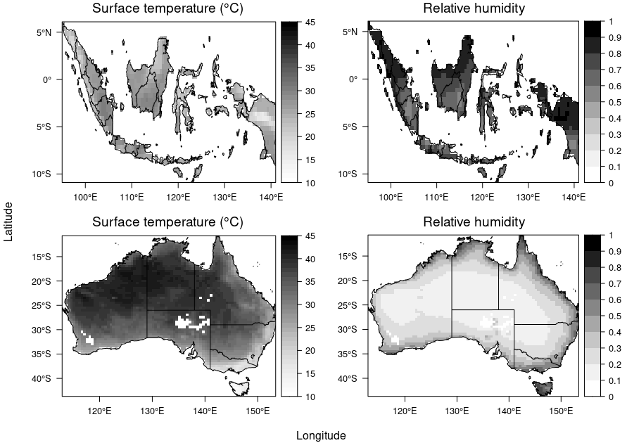
with $T_{0}=273.16$ K, $a_{1}=611.21$ Pa, $a_{3}=17.502$, and $a_{4}=32.19$ K, according to Buck (1981). The data is then re-sampled to match the resolution of our wildfire occurrence dataset using bi-linear interpolation. Figure 3 shows spatial plots of the resulting datasets. Noteworthy here is that there are missing gaps in the dataset—these are artifacts of our preprocessing pipeline, any cells with missing value in any of the covariates were discarded from the analysis (for Indonesia, 3 out of 619 and for Australia, 49 out of 2788).

Figure 4: Preprocessed elevation above sea level (left) and percent tree cover (right) datasets for Indonesia (top) and Australia (bottom).

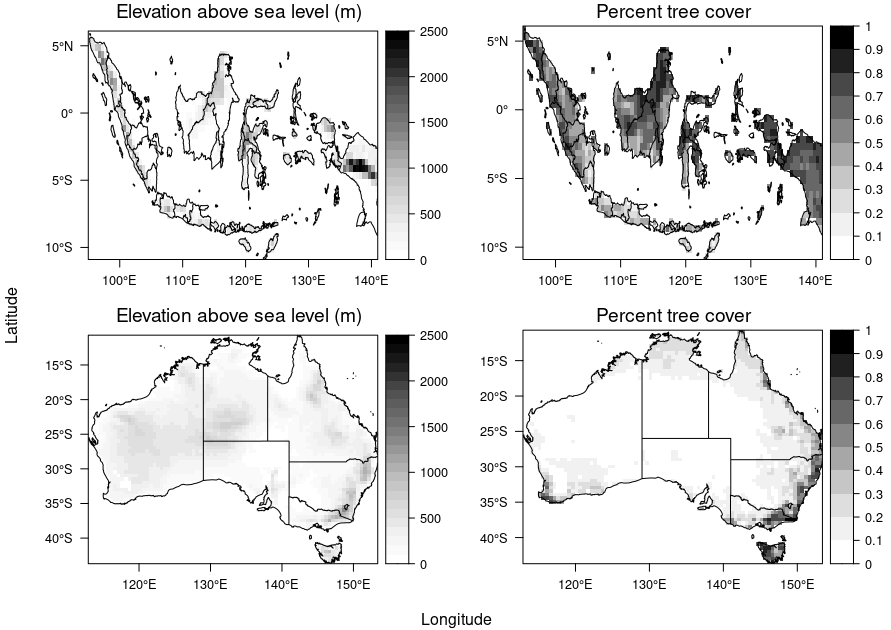
Topographical variables such as elevation above sea level (m) have been shown in some cases to be more important than climate variables (Dillon et al., 2011; Serra et al., 2014). Moreover, Archibald et al. (2009) showed that high percent tree cover (PTC)—defined as the ratio of area covered by branches and tree leaves to ground surface when viewed from above—is a good proxy for high fuel load, thereby allowing fires to propagate more easily than when PTC is low. The datasets were obtained from the Geospatial Information Authority of Japan (Kobayashi et al., 2016; Danielson and Gesch, 2010), and were preprocessed in a similar way to climate variables. Additionally, we had to remove values for sea grids using NCO, as the default values ($-9999$ and $254$ for elevation and PTC respectively) caused the aggregation algorithm to produce wrong values. Figure 4 shows spatial plots of the resulting datasets.

4.2 Results

Using a tolerance level of $\epsilon=1\times 10^{-7}$, the Nelder–Mead algorithm converged at $\hat{\bm{\theta}}_{0}=(0.390,0.518)$ and $\hat{\bm{\theta}}_{+}=(2.565,0.369)$ for the dataset of Indonesia. As mentioned in Section 2.2, since $\tau$ and $\kappa^{2}$ correspond to the inverse relationship variability and strength between latent spatial effects respectively, we can interpret our results as follows. Latent spatial effects for the count process are more strongly correlated with their neighbours than that for the hurdle process $(\hat{\kappa}^{-1}_{+}>\hat{\kappa}^{-1}_{0})$, and the relationship is tighter $(\hat{\tau}^{-1}_{+}>\hat{\tau}^{-1}_{0})$.

Table 1 show the value of the estimated coefficients $\hat{\bm{\beta}}_{0}$ and $\hat{\bm{\beta}}_{+}$ along with their approximate $95\%$ confidence intervals based on asymptotic normality.

Parameter	$\hat{\bm{\beta}}$	Lower C.I.	Upper C.I.	Significant?
$\beta_{0,\text{intercept}}$	56.385	3.638	109.131	TRUE
$\beta_{0,\text{temp}}$	-1.485	-3.456	0.487	FALSE
$\beta_{0,\text{RH}}$	-78.896	-142.910	-14.882	TRUE
$\beta_{0,\text{elev}}$	$2.206\times 10^{-3}$	$-4.554\times 10^{-4}$	$4.868\times 10^{-3}$	FALSE
$\beta_{0,\text{PTC}}$	-2.275	-5.337	0.787	FALSE
$\beta_{0,\text{temp}\cdot\text{RH}}$	2.300	-0.173	4.773	FALSE
$\beta_{+,\text{intercept}}$	15.432	8.763	22.100	TRUE
$\beta_{+,\text{temp}}$	-0.353	-0.589	-0.116	TRUE
$\beta_{+,\text{RH}}$	-20.002	-28.931	-11.074	TRUE
$\beta_{+,\text{elev}}$	$3.468\times 10^{-4}$	$-2.371\times 10^{-4}$	$9.308\times 10^{-4}$	FALSE
$\beta_{+,\text{PTC}}$	-0.490	-1.023	0.043	FALSE
$\beta_{+,\text{temp}\cdot\text{RH}}$	0.567	0.224	0.910	TRUE

Table 1: Estimates of $\hat{\bm{\beta}}_{0}$ and $\hat{\bm{\beta}}_{+}$ when fitting the model to monthly counts of wildfire occurrences in Indonesia on September 2015, approximate $95\%$ confidence intervals based on asymptotic normality and whether they are significantly different from zero.

Parameter	$\hat{\bm{\beta}}$	Lower C.I.	Upper C.I.	Significant?
$\beta_{0,\text{intercept}}$	-2.715	-4.428	-1.002	TRUE
$\beta_{0,\text{temp}}$	-0.048	-0.0932	-0.002	TRUE
$\beta_{0,\text{RH}}$	11.214	-15.126	-7.302	TRUE
$\beta_{0,\text{elev}}$	0.003	0.002	0.004	TRUE
$\beta_{0,\text{PTC}}$	5.279	3.789	6.770	TRUE
$\beta_{0,\text{temp}\cdot\text{RH}}$	0.565	0.457	0.674	TRUE
$\beta_{+,\text{intercept}}$	1.966	0.136	3.796	TRUE
$\beta_{+,\text{temp}}$	-0.045	-0.0935	0.003	FALSE
$\beta_{+,\text{RH}}$	-6.435	-10.271	-2.600	TRUE
$\beta_{+,\text{elev}}$	$5.679\times 10^{-4}$	$8.380\times 10^{-5}$	$1.052\times 10^{-3}$	TRUE
$\beta_{+,\text{PTC}}$	2.254	1.433	3.075	TRUE
$\beta_{+,\text{temp}\cdot\text{RH}}$	0.242	0.131	0.353	TRUE

Table 2: Estimates of $\hat{\bm{\beta}}_{0}$ and $\hat{\bm{\beta}}_{+}$ when fitting the model to monthly counts of wildfire occurrences in Australia on December 2019, along with their $95\%$ confidence intervals and whether they are significantly different from zero.

From Table 1 we have that all else being fixed, a $1\%$ increase in relative humidity at a cell is associated with a $\left(1-\exp(-\color[rgb]{0,0,0}0.789\color[rgb]{0,0,0})\right)\times 100\%=54.57\%$ decrease in the odds of a wildfire occurring at least once on that cell in September 2015, as we had expected. On the other hand and to our surprise, all other hurdle parameters are not significant.

Figure 5: Top: Plots of actual (left) and expected (right) counts of monthly wildfire occurrences. Middle: latent spatial effects $\bm{U}_{0}$ (left) and $\bm{U}_{+}$ (right). Bottom: predicted probabilities of at least one wildfire occurring $\pi(\bm{z}_{i}^{\top}\bm{\beta}_{0}+U_{0i})$ (left), and rate parameters $\lambda(\bm{z}_{i}^{\top}\bm{\beta}_{+}+U_{+i})$ (right) for Indonesia in September 2015.

Figure 6: Top: plots of actual (left) and expected (right) counts of monthly wildfire occurrences. Middle: latent spatial effects $\bm{U}_{0}$ (left) and $\bm{U}_{+}$ (right). Bottom: predicted probabilities of at least one wildfire occurring $\pi(\bm{z}_{i}^{\top}\bm{\beta}_{0}+U_{0i})$ (left), and rate parameters $\lambda(\bm{z}_{i}^{\top}\bm{\beta}_{+}+U_{+i})$ (right) for Australia in December 2019.

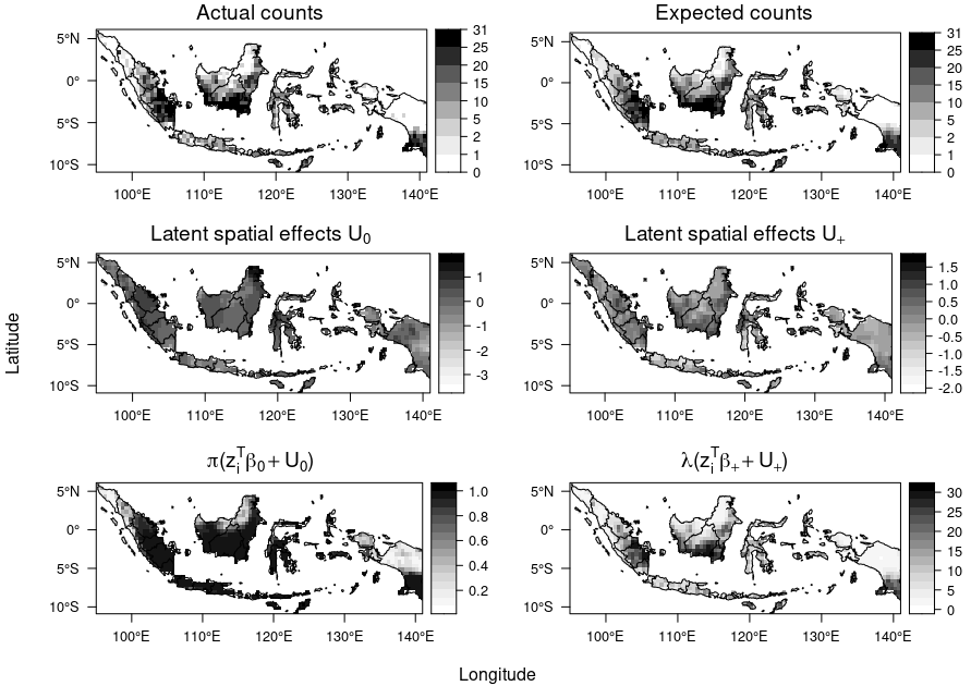
Regarding the count coefficients, we have that else being fixed, a $1\ \text{C}^{\circ}$ increase in surface temperature is associated with a $29.73\%$ decrease in expected count of wildfire occurrences on that cell in September 2015, which is surprising as intuitively we might expect higher surface temperature to be associated with higher counts of wildfire occurrences. The positive magnitude of the interaction term coefficient cannot account for this either; we had expected a lower relative humidity to intensify the effect of temperature on occurrence, but the positive magnitude implies the contrary. This can perhaps be explained by the fact that we do not actually observe any occurrence where surface temperature is high and relative humidity is low; from the bottom-right plot Figure 3, we see that the lowest relative humidity observed in Indonesia is still over $54\%$—any inference involving values below that is simply extrapolation from our part. Figure 5 shows that the pattern of the predicted counts largely matches with those in the actual counts, which is usually a good sign that the model fit is adequate. However, it appears that our model are predicting small wildfires (light grey) for cells with no wildfires (dark grey) in the top-left and top-centre. This could be an artifact of our dependency structure where any cell always depends on its neighbours, forcing the spatial effects to be smooth all over the region. This is also shown in the middle-left and middle-right plot, which shows that the transition from regions with low or negative spatial effects to regions with large spatial effects is gradual.

Comparing Figure 3 with the bottom-left and bottom-right plots in Figure 5, we observe that the inverse of the pattern in relative humidity are similar to the pattern in predicted probabilities and rate parameters, which helps to partially explain the negative sign of the coefficients. On the other hand, it would appear that the relationship between surface temperature and predicted probabilities and rate parameters are not as obvious. Figure 7 on the left shows the receiver operating characteristic (ROC) curve of the fitted model. We conclude that our model can discriminate between cells with at least one wildfire occurrence and cells with no wildfire occurrence very well, but this is not surprising at all given that these are in-sample predictions. The high AUC value also confirms our visual inspection that the red spots in the bottom-left plot of Figure 5 match closely with the non-white spots in the upper-right plot of the same figure.

Figure 7: (Left): ROC curve of the hurdle part of the fitted Indonesian (top) model and Australian (bottom) model. The shape of the curve and the high area under curve (AUC) value indicates that our model can discriminate between positive and zero cells very well. (Right): Plot of Pearson residuals against expected counts of wildfire occurrences for Indonesian model. The negative deviations for small expected counts suggest our model consistently over-predicts the number of occurrences for observations with small actual counts.

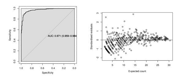
On the other hand, Figure 7 on the right shows a plot of the Pearson residuals against expected counts of wildfire occurrences. The plots show that Pearson residuals for cells with expected counts of $10$ or less are overwhelmingly negative, indicating that our model has a tendency to over-predict the number of wildfire occurrences in cells with few observed counts. This also confirms our observation that the latent spatial effects are smooth over the entire domain, whereas the actual data comprises more abrupt boundaries of fire and no-fire zones. This is not necessarily a bad thing, as our model essentially provides a more conservative threshold for when a zone should be declared as high risk. Furthermore, our main concern are cells with high counts of wildfire occurrences, where the deviations are not as large.

Due to computational limitations, we used a tolerance level of $\epsilon=1\times 10^{-3}$ in our analysis. The Nelder–Mead converged at $\hat{\bm{\theta}}_{0}=\left(1.299,1.326\right)$ and $\hat{\bm{\theta}}_{+}=\left(0.826,0.481\right)$ for the dataset of Australia. We can interpret $\hat{\bm{\theta}}$ in a similar fashion to what we did in Section 4.2 to arrive at the same conclusion, although we must emphasize again that our conclusion is subject to the reliability of our estimate $\hat{\bm{\theta}}$.

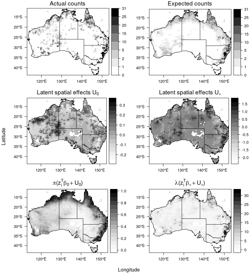
Table 2 show the value of the estimated coefficients $\hat{\bm{\beta}}_{0}$ and $\hat{\bm{\beta}}_{+}$ along with their $95\%$ confidence intervals, which can be interpreted in the same manner as in Section 4.2. What is noteworthy here is the differing signs in the coefficients of relative humidity for the hurdle and count part. While higher humidity is associated with lower counts of wildfire occurrences, as have been empirically shown, it would appear that higher humidity is associated with a higher probability of a wildfire occurring at least once. This is perhaps less surprising once we compare the bottom-right plot of Figure 3 and the bottom-left plot of Figure 6: in our dataset, wildfire occurrences are almost guaranteed along the coastal areas, which also happens to be areas with high relative humidity. Without further research one can only speculate, but a reasonable guess would be that areas with low relative humidity in Australia tend to be deserts with very few materials that can act as a fuel for fires to ignite and propagate. This is partially supported by the bottom-right plot of Figure 4, which shows that these areas have low PTC values. It is also interesting to note that surface temperature and the interaction term show similar effects to the one observed in Section 4.2. This perhaps highlight an important weakness of our climate dataset; using aggregated monthly averages as our covariates caused us to lose a substantial amount of information regarding inter-month fluctuations, so our current results could very well be an exemplification of ecological bias also known as Simpson’s paradox (Simpson, 1951), which loosely speaking highlights the danger of simply relying on aggregate data, which could mask and obscure actual effects.

Here, the pattern of predicted counts do not match as well as those in the actual counts.  The smoothness of the latent spatial effects is even more apparent here; in the top-right plot in Figure 6 we observe that our model has essentially linked together three separate clusters of fires in the north-west, north-east, and south-east, into one smooth curve that traces the coastline from the top left corner all the way to the bottom-right corner of Australia. Another interesting observation to make is that our latent spatial effects $\hat{\bm{U}}_{+}$ for the hurdle part picked up on the wildfire occurrences in the Western Australia, which our covariates were not able to account for. This is shown in the middle-left plot in Figure 6, where there are black spots in the middle-left area, but not along the coast, since our covariates can account for those. This highlights the advantage of spatial Poisson hurdle models have over vanilla Poisson hurdle models described in Section 2.

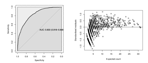
Figure 7 on the left shows the ROC curve of the fitted model, and shows that our model is not as discriminative as the one fitted to the data for Indonesia. This largely matches what we observed in the bottom-left plot of Figure 6, and can be attributed to the fact that the covariates were not able to account for why there are occurrences of wildfires in Central Australia. As a result, our model did not assign a high probability of at least one observation of wildfire occurrence in these areas. Meanwhile, Figure 7 on the right show that as a result of the smoothness of the latent spatial effects, our model has not only the tendency to over-predict the number of wildfire occurrences in cells with few observed counts, but also under-predict the number of wildfire occurrences in cells with large observed counts. This is more worrying, since our model risks providing an overly optimistic threshold and gloss over what would have actually been a high risk zone.

Overall, we conclude that globally smooth latent spatial effects may lack flexibility in modelling geographical variation in monthly counts of wildfire occurrences. As such, potential future work include exploring methods to constraint the latent spatial effects to not be globally smooth as for example in Lee et al. (2014) who proposed a localized conditional auto-regressive prior for modelling residual spatial auto-correlation, which could serve as a good starting point for this endeavour. Another potential avenue for further research would be to investigate a latent temporal process for modelling variation in wildfire occurrences in a single area over time, and finally combining it with the existing spatial model to create a spatio-temporal model for modelling counts of wildfire occurrences.

Appendix A Optimization methods

A.1 Optimization of approximate marginal posterior

To maximize the approximate marginal posterior distribution given by expression (9) we implement the downhill simplex method of Nelder and Mead (1965). In particular, we maximize rCl log~f(θ∣y) &= logf(θ) + logf(x ∣θ) + logL(x ∣y, z) - log~f_G(x ∣θ, y). Additionally, the iterative scheme given by (10) requires computation of the gradient and Hessian of the full conditional density $\log f(\bm{x}\mid\bm{\theta},\bm{y})$. Here we note that, by linearity of gradient operator $\nabla_{\bm{x}}$ and Hessian operator $\nabla_{\bm{x}}\nabla_{\bm{x}}^{\top}$ and the fact that $f(\bm{x}\mid\bm{\theta},\bm{y})\propto L(\bm{x}\mid\bm{y},\bm{z})\,f(\bm{x}\ |\ \bm{\theta})$, computation of the gradient and Hessian of the full conditional simply reduces to

$$\nabla_{\bm{x}}\log f(\bm{x}\mid\bm{\theta},\bm{y}) =\nabla_{\bm{x}}\log f(\bm{y}\mid\bm{x})+\nabla_{\bm{x}}\log f(\bm{x}\mid\bm{\theta}),\text{ and}$$

$$\nabla_{\bm{x}}\nabla_{\bm{x}}^{\top}\log f(\bm{x}\mid\bm{\theta},\bm{y}) =\nabla_{\bm{x}}\nabla_{\bm{x}}^{\top}\log f(\bm{y}\mid\bm{x})+\nabla_{\bm{x}}\nabla_{\bm{x}}^{\top}\log f(\bm{x}\mid\bm{\theta}),$$

where $\nabla_{\bm{x}}\log f(\bm{x}\mid\bm{\theta})=-Q(\bm{\theta})\,(\bm{x}-\bm{\mu}),\quad\nabla_{\bm{x}}\nabla_{\bm{x}}^{\top}\log f(\bm{x}\mid\bm{\theta})=-Q(\bm{\theta})$. The log-likelihood together with its gradient vector $\nabla_{\bm{x}}\log L(\bm{x}\mid\bm{y},\bm{z})$ and Hessian matrix $\nabla_{\bm{x}}\nabla_{\bm{x}}^{\top}\log L(\bm{x}\mid\bm{y},\bm{z})$ are given in Appendix A.2, A.3 and Appendix A.4 respectively.

A.2 Log-likelihood

The logarithm of the likelihood function $L(\bm{x}\mid\bm{y},\bm{z})$ given by expression (7) is

$$\ell(\bm{x};\bm{y},\bm{z})=\sum_{i=1}^{n}\mathbbm{1}_{\{y_{i}=0\}}\log{\{1-\pi(\bm{z}_{i}^{\top}\bm{\beta}_{0}+U_{0i})\}}+\sum_{i=1}^{n}\mathbbm{1}_{\{y_{i}>0\}}\log{\{\pi(\bm{z}_{i}^{\top}\bm{\beta}_{0}+U_{0i})\}}\\ +\sum_{i=1}^{n}\mathbbm{1}_{\{y_{i}>0\}}\,y_{i}\,(\bm{z}_{i}^{\top}\bm{\beta}_{+}+U_{+i})-\sum_{i=1}^{n}\mathbbm{1}_{\{y_{i}>0\}}\lambda(\bm{z}_{i}^{\top}\bm{\beta}_{+}+U_{+i})\\ -\sum_{i=1}^{n}\mathbbm{1}_{\{y_{i}>0\}}\log{(y_{i}!)}-\sum_{i=1}^{n}\mathbbm{1}_{\{y_{i}>0\}}\log{[1-\exp\{-\lambda(\bm{z}_{i}^{\top}\bm{\beta}_{+}+U_{+i})\}]}.$$ (14)

A.3 Gradient vector of Poisson hurdle log-likelihood

Routine differentiation of (14) gives

$$\dfrac{\partial\ell}{\partial\beta_{0p}} =\sum_{i=1}^{n}z_{ip}\left[\dfrac{\mathbbm{1}_{\{y_{i}>0\}}}{1+\exp{(\bm{z}_{i}^{\top}\bm{\beta}_{0}+U_{0i})}}-\dfrac{\mathbbm{1}_{\{y_{i}=0\}}}{1+\exp{\{-(\bm{z}_{i}^{\top}\bm{\beta}_{0}+U_{0i})\}}}\right],$$

$$\dfrac{\partial\ell}{\partial\beta_{+p}} =\sum_{i=1}^{n}z_{ip}\mathbbm{1}_{\{y_{i}>0\}}\left[y_{i}-\exp(\bm{z}_{i}^{\top}\bm{\beta}_{+}+U_{+i})-\dfrac{\exp(\bm{z}_{i}^{\top}\bm{\beta}_{+}+U_{+i})}{\exp\{\exp(\bm{z}_{i}^{\top}\bm{\beta}_{+}+U_{+i})\}-1}\right],$$

$$\dfrac{\partial\ell}{\partial U_{0i}} =\dfrac{\mathbbm{1}_{\{y_{i}>0\}}}{1+\exp{(\bm{z}_{i}^{\top}\bm{\beta}_{0}+U_{0i})}}-\dfrac{\mathbbm{1}_{\{y_{i}=0\}}}{1+\exp{\{-(\bm{z}_{i}^{\top}\bm{\beta}_{0}+U_{0i})\}}},\text{ and}$$

$$\dfrac{\partial\ell}{\partial U_{+i}} =\mathbbm{1}_{\{y_{i}>0\}}\left\{y_{i}-\exp(\bm{z}_{i}^{\top}\bm{\beta}_{+}+U_{+i})-\dfrac{\exp(\bm{z}_{i}^{\top}\bm{\beta}_{+}+U_{+i})}{\exp\{\exp(\bm{z}_{i}^{\top}\bm{\beta}_{+}+U_{+i})\}-1}\right\},$$

where $p=0,\dots,k$ and $i=1,\ldots,n$.

A.4 Hessian matrix of Poisson hurdle log-likelihood

Routine differentiation of (14) gives

$$\dfrac{\partial^{2}\ell}{\partial\beta_{0q}\partial\beta_{0p}} =-\sum_{i=1}^{n}\dfrac{z_{ip}z_{iq}}{\eta_{0}^{\prime}+{\eta_{0}^{\prime}}^{-1}+2},$$

$$\dfrac{\partial^{2}\ell}{\partial\beta_{+q}\partial\beta_{+p}} =\sum_{i=1}^{n}z_{ip}z_{iq}\mathbbm{1}_{\{y_{i}>0\}}\left[\dfrac{\eta_{+}^{\prime}\left\{(\eta_{+}^{\prime}-1)\exp(\eta_{+}^{\prime})+1\right\}}{\left[\exp(\eta_{+}^{\prime})-1\right]^{2}}-\eta_{+}^{\prime}\right],$$

$$\dfrac{\partial^{2}\ell}{\partial\beta_{0p}\partial U_{0i}} =-\dfrac{z_{ip}}{\eta_{0}^{\prime}+{\eta_{0}^{\prime}}^{-1}+2},$$

$$\dfrac{\partial^{2}\ell}{\partial\beta_{+p}\partial U_{+i}} =z_{ip}\mathbbm{1}_{\{y_{i}>0\}}\left[\dfrac{\eta_{+}^{\prime}\left\{(\eta_{+}^{\prime}-1)\exp(\eta_{+}^{\prime})+1\right\}}{\left\{\exp(\eta_{+}^{\prime})-1\right\}^{2}}-\eta_{+}^{\prime}\right],$$

$$\dfrac{\partial^{2}\ell}{\partial U_{0i}^{2}} =-\dfrac{1}{\eta_{0}^{\prime}+{\eta_{0}^{\prime}}^{-1}+2},$$

$$\dfrac{\partial^{2}\ell}{\partial U_{+i}^{2}} =\mathbbm{1}_{\{y_{i}>0\}}\left[\dfrac{\eta_{+}^{\prime}\left\{(\eta_{+}^{\prime}-1)\exp(\eta_{+}^{\prime})+1\right\}}{\left\{\exp(\eta_{+}^{\prime})-1\right\}^{2}}-\eta_{+}^{\prime}\right],\text{ and}$$

$$\dfrac{\partial^{2}\ell}{\partial\beta_{+q}\partial U_{0p}} =\dfrac{\partial^{2}\ell}{\partial\beta_{0q}\partial U_{+p}}=\dfrac{\partial^{2}\ell}{\partial\beta_{+q}\partial\beta_{0p}}=\dfrac{\partial^{2}\ell}{\partial U_{+j}\partial U_{0i}}=0,$$

where $\eta_{0}^{\prime}=\exp(\bm{z}_{i}^{\top}\bm{\beta}_{0}+U_{0i})$ and $\eta_{+}^{\prime}=\exp(\bm{z}_{i}^{\top}\bm{\beta}_{+}+U_{+i})$, $p,q=0,\dots,k$ and $i=1,\ldots,n$.

A.5 Newton’s method for optimization

  Inputs: hyper-parameter $\bm{\theta}$, response variable $\bm{y}$, covariates $\bm{z}$, tolerance level $\epsilon$;

  Initialize $\bm{x}^{(0)}\leftarrow\bm{0}$;

  Initialize step size $\alpha\leftarrow 1$;

  for $t=0,1,2,\dots$ do

     $\bm{x}^{(t+1)}\leftarrow\bm{x}^{(t)}-\alpha\left[-\nabla_{\bm{x}}\nabla_{\bm{x}}^{\top}\log f\{\bm{x}^{(0)}\}\right]^{-1}\nabla_{\bm{x}}\log f\{\bm{x}^{(0)}\}$;

     while $\log f\{\bm{x}^{(t+1)}\}<\log f\{\bm{x}^{(t)}\}$ do

         $\alpha\leftarrow\alpha/2$;

         $\bm{x}^{(t+1)}\leftarrow\bm{x}^{(t)}-\alpha\left[-\nabla_{\bm{x}}\nabla_{\bm{x}}^{\top}\log f\{\bm{x}^{(0)}\}\right]^{-1}\nabla_{\bm{x}}\log f\{\bm{x}^{(0)}\}$;

         if $\alpha\leq 2^{-9}$ then

            stop and let $\bm{x}^{(t+1)}\leftarrow\bm{x}^{(t)}$;

         end if

     end while

     if $\left|\left\|\bm{x}^{(t+1)}\right\|-\left\lVert\bm{x}^{(t)}\right\lVert\right|<\epsilon$ then

         stop and return $\bm{x}^{(t+1)}$;

     end if

  end for

Algorithm 1 Newton’s method; for brevity $f(\bm{x})\equiv f(\bm{x}\mid\bm{\theta},\bm{y})$.

References

- (1)
- Archibald et al. (2009) Archibald, S., Roy, D. P., van Wilgen, B. W. and Scholes, R. J. (2009), ‘What limits fire? An examination of drivers of burnt area in Southern Africa’, Global Change Biology 15(3), 613–630.
- Besag (1974) Besag, J. (1974), ‘Spatial interaction and the statistical analysis of lattice systems’, Journal of the Royal Statistical Society. Series B (Methodological) 36(2), 192–236.
- Boucher et al. (2007) Boucher, J.-P., Denuit, M. and Guillén, M. (2007), ‘Risk classification for claim counts’, North American Actuarial Journal 11(4), 110–131.
- Bu and Gharajeh (2019) Bu, F. and Gharajeh, M. S. (2019), ‘Intelligent and vision-based fire detection systems: A survey’, Image and Vision Computing 91, 103803.
- Buck (1981) Buck, A. L. (1981), ‘New equations for computing vapor pressure and enhancement factor’, Journal of Applied Meteorology 20(12), 1527–1532.
- Copernicus Climate Change Service (2017) Copernicus Climate Change Service (2017), ‘ERA5: Fifth generation of ECMWF atmospheric reanalyses of the global climate’. Data retrieved from the Copernicus Climate Change Service Climate Data Store (CDS) on 14 Jan 2020.
- Danielson and Gesch (2010) Danielson, J. J. and Gesch, D. B. (2010), Global multi-resolution terrain elevation data 2010 (GMTED2010). Preprocessed by the Geospatial Information Authority of Japan.
- Dickman (2020) Dickman, C. (2020), ‘More than one billion animals impacted in Australian bushfires’.
- Dillon et al. (2011) Dillon, G. K., Holden, Z. A., Morgan, P., Crimmins, M. A., Heyerdahl, E. K. and Luce, C. H. (2011), ‘Both topography and climate affected forest and woodland burn severity in two regions of the western US, 1984 to 2006’, Ecosphere 2(12), 1–33.
- ECMWF (2016) ECMWF (2016), Part IV: Physical Processes, number 4 in ‘IFS Documentation’, ECMWF.
- Flannigan and Harrington (1988) Flannigan, M. and Harrington, J. (1988), ‘A study of the relation of meteorological variables to monthly provincial area burned by wildfire in Canada (1953–80)’, Journal of Applied Meteorology 27(4), 441–452.
- GDAL/OGR contributors (2020) GDAL/OGR contributors (2020), GDAL/OGR Geospatial Data Abstraction software Library, Open Source Geospatial Foundation.
- Hijmans (2019) Hijmans, R. J. (2019), raster: Geographic Data Analysis and Modeling. R package version 3.0-7.
- Hoque et al. (2017) Hoque, M. A.-A., Phinn, S., Roelfsema, C. and Childs, I. (2017), ‘Tropical cyclone disaster management using remote sensing and spatial analysis: A review’, International journal of disaster risk reduction 22, 345–354.
- Huijnen et al. (2016) Huijnen, V., Wooster, M. J., Kaiser, J. W., Gaveau, D. L., Flemming, J., Parrington, M., Inness, A., Murdiyarso, D., Main, B. and Van Weele, M. (2016), ‘Fire carbon emissions over maritime Southeast Asia in 2015 largest since 1997’, Scientific Reports 6, 26886.
- Jha et al. (2008) Jha, M. N., Levy, J. and Gao, Y. (2008), ‘Advances in remote sensing for oil spill disaster management: state-of-the-art sensors technology for oil spill surveillance’, Sensors 8(1), 236–255.
- Jolly et al. (2015) Jolly, W. M., Cochrane, M. A., Freeborn, P. H., Holden, Z. A., Brown, T. J., Williamson, G. J. and Bowman, D. M. (2015), ‘Climate-induced variations in global wildfire danger from 1979 to 2013’, Nature communications 6(1), 1–11.
- Kaiser et al. (2012) Kaiser, J. W., Heil, A., Andreae, M. O., Benedetti, A., Chubarova, N., Jones, L., Morcrette, J.-J., Razinger, M., Schultz, M. G., Suttie, M. and van der Werf, G. R. (2012), ‘Biomass burning emissions estimated with a global fire assimilation system based on observed fire radiative power’, Biogeosciences 9(1), 527–554.
- Ko and Kwak (2012) Ko, B. and Kwak, S. (2012), ‘Survey of computer vision-based natural disaster warning systems’, Optical Engineering 51(7), 1 – 12.
- Kobayashi et al. (2016) Kobayashi, T., Tsend-Ayush, J. and Tateishi, R. (2016), ‘A new global tree-cover percentage map using MODIS data’, International Journal of Remote Sensing 37(4), 969–992.
- Lee et al. (2014) Lee, D., Rushworth, A. and Sahu, S. K. (2014), ‘A Bayesian localized conditional autoregressive model for estimating the health effects of air pollution’, Biometrics 70(2), 419–429.
- Lewis (2020) Lewis, D. (2020), “Deathly silent’: Ecologist describes Australian wildfires’ devastating aftermath.’, Nature 577(7790), 304.
- Mahmoud and Ren (2018) Mahmoud, M. A. and Ren, H. (2018), ‘Forest fire detection using a rule-based image processing algorithm and temporal variation’, Mathematical Problems in Engineering 2018.
- Marlier et al. (2013) Marlier, M. E., DeFries, R. S., Voulgarakis, A., Kinney, P. L., Randerson, J. T., Shindell, D. T., Chen, Y. and Faluvegi, G. (2013), ‘El Niño and health risks from landscape fire emissions in Southeast Asia’, Nature climate change 3(2), 131–136.
- Neelon et al. (2013) Neelon, B., Ghosh, P. and Loebs, P. F. (2013), ‘A spatial Poisson hurdle model for exploring geographic variation in emergency department visits’, Journal of the Royal Statistical Society: Series A (Statistics in Society) 176(2), 389–413.
- Nelder and Mead (1965) Nelder, J. A. and Mead, R. (1965), ‘A simplex method for function minimization’, The Computer Journal 7(4), 308–313.
- Nocedal and Wright (2006) Nocedal, J. and Wright, S. (2006), Numerical Optimization, Springer Science & Business Media.
- Rohrbeck et al. (2018) Rohrbeck, C., Eastoe, E. F., Frigessi, A., Tawn, J. A. et al. (2018), ‘Extreme value modelling of water-related insurance claims’, The Annals of Applied Statistics 12(1), 246–282.
- Rue and Held (2005) Rue, H. and Held, L. (2005), Gaussian Markov random fields: theory and applications, CRC press.
- Schulzweida (2019) Schulzweida, U. (2019), ‘CDO user guide’. doi: 10.5281/zenodo.3539275.
- Serra et al. (2014) Serra, L., Saez, M., Juan, P., Varga, D. and Mateu, J. (2014), ‘A spatio-temporal Poisson hurdle point process to model wildfires’, Stochastic Environmental Research and Risk Assessment 28(7), 1671–1684.
- Simpson (1951) Simpson, E. H. (1951), ‘The interpretation of interaction in contingency tables’, Journal of the Royal Statistical Society: Series B (Methodological) 13(2), 238–241.
- Tierney and Kadane (1986) Tierney, L. and Kadane, J. B. (1986), ‘Accurate approximations for posterior moments and marginal densities’, Journal of the American Statistical Association 81(393), 82–86.
- Unidata (2020) Unidata (2020), ‘Network Common Data Form (netCDF) version 4.3.3.1 [software]’. Boulder, CO: UCAR/Unidata.
- Wooster et al. (2005) Wooster, M. J., Roberts, G., Perry, G. and Kaufman, Y. (2005), ‘Retrieval of biomass combustion rates and totals from fire radiative power observations: FRP derivation and calibration relationships between biomass consumption and fire radiative energy release’, Journal of Geophysical Research: Atmospheres 110(D24).
- Zeileis et al. (2008) Zeileis, A., Kleiber, C. and Jackman, S. (2008), ‘Regression models for count data in R’, Journal of Statistical Software 27(8).
- Zender (2020) Zender, C. S. (2020), ‘netCDF Operator (NCO) User Guide, Version 4.9.3’.