Hamiltonicity of the Double Vertex Graph and the
Complete Double Vertex Graph of some Join Graphs

Abstract

Let $G$ be a simple graph of order $n$. The double vertex graph $F_{2}(G)$ of $G$ is the graph whose vertices are the $2$-subsets of $V(G)$, where two vertices are adjacent in $F_{2}(G)$ if their symmetric difference is a pair of adjacent vertices in $G$. A generalization of this graph is the complete double vertex graph $M_{2}(G)$ of $G$, defined as the graph whose vertices are the $2$-multisubsets of $V(G)$, and two of such vertices are adjacent in $M_{2}(G)$ if their symmetric difference (as multisets) is a pair of adjacent vertices in $G$. In this paper we exhibit an infinite family of graphs (containing Hamiltonian and non-Hamiltonian graphs) for which $F_{2}(G)$ and $M_{2}(G)$ are Hamiltonian. This family of graphs is the set of join graphs $G=G_{1}+G_{2}$, where $G_{1}$ and $G_{2}$ are of order $m\geq 1$ and $n\geq 2$, respectively, and $G_{2}$ has a Hamiltonian path. For this family of graphs, we show that if $m\leq 2n$ then $F_{2}(G)$ is Hamiltonian, and if $m\leq 2(n-1)$ then $M_{2}(G)$ is Hamiltonian.

1 Introduction.

Throughout this paper, $G$ is a simple graph of order $n\geq 2$. In this paper we deal with two constructions of graphs, the double vertex graph and the complete double vertex graph. The $k$-token graph $F_{k}(G)$ of $G$ is the graph whose vertices are the $k$-subsets of $V(G)$, where two of such vertices are adjacent if their symmetric difference is a pair of adjacent vertices in $G$. The $k$-multiset graph $M_{k}(G)$ of $G$ is the graph whose vertices are the $k$-multisubsets of $V(G)$, and two of such vertices are adjacent if their symmetric difference (as multisets) is a pair of adjacent vertices in $G$. See an example of these constructions in Figure 1. The $2$-token graph is usually called the double vertex graph and the $2$-multiset graph is called the complete double vertex graph.

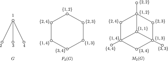
Figure 1: A graph $G$, its double vertex graph $F_{2}(G)$ and its complete double vertex graph $M_{2}(G)$.

The $k$-token graphs have been defined, independently, at least four times, see [2, 16, 22, 30]. A classical example of token graphs is the Johnson graph $J(n,k)$ that is, in fact, the $k$-token graph of the complete graph $K_{n}$. The Johnson graphs have been widely studied in the last three decades due to its connections with coding theory, see for example [15, 23, 27]. The $k$-multiset graph was introduced in 2001 by Chartrand et al. [12].

In 1988, Johns defined the $k$-token graphs in his PhD thesis under the name of the $k$-subgraph graph, and he studied some combinatorial properties of these graphs.

In 1991, Alavi et al. reintroduced, independently, the $2$-token graphs, calling them the double vertex graphs, and they studied combinatorial properties of these graphs, such as connectivity, planarity, regularity and Hamiltonicity, see [2, 3, 4, 5, 32].

Several years later, Rudolph [9, 30] redefined the token graphs, with the name of symmetric powers of graphs, with the aim to study the graph isomorphism problem and for its possible applications to quantum mechanics. Rudolph gave several examples of cospectral non-isomorphic graphs such that the corresponding $2$-token graphs are non-cospectral. This shows that, sometimes, the spectrum of the $2$-token graph of $G$ is a better invariant than the spectrum of $G$. However, Alzaga et al. [8] and, independently, Barghi and Ponomarenko [10] proved that for any positive integer $k\geq 2$ there exists infinitely many pairs of non-isomorphic graphs with cospectral $k$-token graphs. Several authors have continued with the study of the possible applications of the token graphs in physics (see. e.g., [18, 19, 26]).

Fabila-Monroy et al., [16] reintroduced the concept of $k$-token graph of $G$ as a model in which $k$ indistinguishable tokens move on the vertices of a graph $G$ along the edges of $G$. They began a systematic study of some combinatorial parameters of $F_{k}(G)$ such as connectivity, diameter, cliques, chromatic number, Hamiltonian paths and Cartesian product. This line of research has been continued by different authors, see, e.g., [6, 13, 14, 17, 20, 24, 25]. In particular Soto et al., [20] showed that a problem in coding theory is equivalent to the study of the packing number of the token graphs of the path graph.

For two disjoint graphs $G_{1}$ and $G_{2}$, the join graph $G=G_{1}+G_{2}$ of graphs $G_{1}$ and $G_{2}$ is the graph whose vertex set is $V(G_{1})\cup V(G_{2})$ and its edge set is $E(G_{1})\cup E(G_{2})\cup\{uv:u\in G_{1}\text{ and }v\in G_{2}\}$, a simple example is the complete bipartite graph $K_{m,n}=E_{m}+E_{n}$, where $E_{r}$ denotes the graph of $r$ isolated vertices. The graph $F_{m,n}=E_{m}+P_{n}$ is called the fan graph, where $P_{n}$ denotes the path graph of $n$ vertices (see an example in Figure 2 (left)).

A Hamiltonian path (resp. a Hamiltonian cycle) of a graph $G$ is a path (resp. cycle) containing each vertex of $G$ exactly once. A graph $G$ is Hamiltonian if it contains a Hamiltonian cycle. In this paper we show the following result for the fan graphs.

Theorem 1.

Let $m\geq 1$ and $n\geq 2$. Then, $F_{2}(F_{m,n})$ is Hamiltonian if and only if $m\leq 2n$, and $M_{2}(F_{m,n})$ is Hamiltonian if and only if $m\leq 2(n-1)$.

With the aim of clarity in the exposition of the proof, this theorem has been separated in next subsection as Theorem 1.1 and Theorem 1.2. The proof of Theorem 1.1 was published in [1] (Theorem 1) and the proof of Theorem 1.2 was published in [28].

This theorem implies easily the following more general result.

Corollary 2.

Let $G_{1}$ and $G_{2}$ be two graphs of order $m\geq 1$ and $n\geq 2$, respectively, such that $G_{2}$ has a Hamiltonian path. Let $G=G_{1}+G_{2}$. If $m\leq 2n$ then $F_{2}(G)$ is Hamiltonian, and if $m\leq 2(n-1)$ then $M_{2}(G)$ is Hamiltonian.

So far, the families of graphs for which it has been studied the Hamiltonicity of their double vertex graphs and their complete double vertex graphs are the following: complete bipartite graphs or graphs that have a Hamiltonian path. We point out that the infinite family of graphs given by Corollary 2 contains an infinity number of non-Hamiltonian graphs for which their double vertex graphs and complete double vertex graphs are Hamiltonian, for example, as we are going to show, if $n+1\leq m\leq 2n$ (resp. $n+1\leq m\leq 2(n-1)$) then $F_{m,n}$ is non-Hamiltonian while its double vertex graph $F_{2}(F_{m,n})$ (resp. its complete double vertex graph $M_{2}(F_{m,n})$) is Hamiltonian.

1.1 Hamiltonicity of double and complete double vertex graphs

It is well known that the Hamiltonicity of $G$ does not imply the Hamiltonicity of $F_{k}(G)$. For example, for the complete bipartite graph $K_{m,m}$, Fabila-Monroy et al. [16] showed that if $k$ is even, then $F_{k}(K_{m,m})$ is non-Hamiltonian. A more easy and traditional example is the case of a cycle graph. It is known that if $n=4$ or $n\geq 6$, then $F_{2}(C_{n})$ is not Hamiltonian. On the other hand, there exist non-Hamiltonian graphs for which its double vertex graph is Hamiltonian, a simple example is the graph $K_{1,3}$, for which $F_{2}(K_{1,3})\simeq C_{6}$, and so $F_{2}(K_{1,3})$ is Hamiltonian.

Next, we list the known results about the Hamiltonicity of $F_{k}(G)$ or the existence of a Hamiltonian path in $F_{k}(G)$, when $k$ may be greater than two.

• If $n\geq 3$ and $1\leq k\leq n-1$, then $F_{k}(K_{n})$ is Hamiltonian, see for example [7].

• If $m\geq 2$, then $F_{k}(K_{m,m})$ has a Hamiltonian path if and only if $k$ is odd [16].

• If $G$ is a graph containing a Hamiltonian path and $n$ is even and $k$ is odd, then $F_{k}(G)$ has a Hamiltonian path [16].

• If $n\geq 3$ and $1\leq k\leq n-1$, then $F_{k}(F_{1,n-1})$ is Hamiltonian [29].

In addition to these results, the following are some known results for the double vertex graph ($k=2$).

• $F_{2}(C_{n})$ is non-Hamiltonian [5].

• If $G$ is a cycle with an odd chord, then $F_{2}(G)$ is Hamiltonian [5].

• $F_{2}(K_{m,n})$ is Hamiltonian if and only if $(m-n)^{2}=m+n$ [5].

More results about the Hamiltonicity of double vertex graphs can be found in the survey of Alavi et. al. [4]. We point out that the graphs for which have been studied the Hamiltonicity of its $k$-token graph (even for $k=2$) are Hamiltonian or have a Hamiltonian path or are complete bipartite graphs.

As we mentioned before, in 2018 [29] the last two authors of this article showed the following result: if $n\geq 3$, and $1\leq k\leq n-1$, then the $k$-token graph of the fan graph $F_{1,n-1}$ is Hamiltonian. We have continued with this line of research and in this work we show the following result for the double vertex graph of fan graphs.

Theorem 1.1 ([1], Theorem 1).

The double vertex graph of $F_{m,n}$ is Hamiltonian if and only if $n\geq 2$ and $1\leq m\leq 2\,n$, or $n=1$ and $m=3$.

In Figure 2 we show the double vertex graph of the fan graph $F_{3,3}$ (center) and a Hamiltonian cycle in such graph (right).

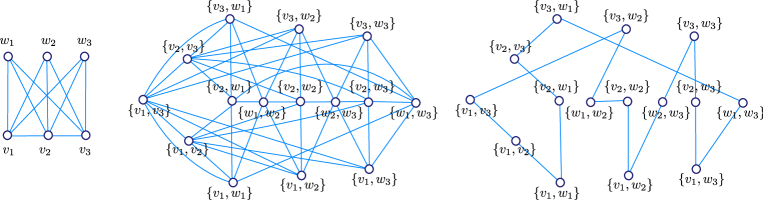
Figure 2: The graph $F_{3,3}$ (left), its double vertex graph (center) and a Hamiltonian cycle in such graph (right).

Let us now turn our attention to the complete double vertex graph. Complete double vertex graphs were implicitly presented in the work of Chartrand et al. [12], and in an explicit way by Jacob et. al. [21], were their first combinatorial properties were studied, and are a generalization of the double vertex graphs.

As far as we know, only the following two results are known about the Hamiltonicity of $M_{2}(G)$.

• For $n\geq 4$, $M_{2}(C_{n})$ is non-Hamiltonian [21].

• If $G$ is obtained from a cycle of $n$ vertices by adding a chord between two vertices at distance two, then $M_{2}(G)$ is Hamiltonian [21].

In this paper we show the following result for the Hamiltonicity of complete double vertex graphs.

Theorem 1.2 ([28], Theorem 1).

The complete double vertex graph of $F_{m,n}$ is Hamiltonian if and only if $n\geq 2$ and $1\leq m\leq 2\,(n-1)$.

As we mentioned before, we have splitted Theorem 1 into Theorems 1.1 and 1.2, and Corollary 2 follows easily from Theorem 1. The infinite family of graphs given in Corollary 2 contains an infinite number of non-Hamiltonian graphs for which their double vertex graph and complete double vertex graph are Hamiltonian, for example, for the fan graph $F_{m,n}$ we know that $F_{m,n}$ is Hamiltonian if and only if $1\leq m\leq n$, while, as we are going to show, $F_{2}(F_{m,n})$ (resp. $M_{2}(F_{m,n})$) is Hamiltonian if and only if $1\leq m\leq 2n$ (resp. $1\leq m\leq 2(n-1)$).

The rest of the paper is organized as follows. In Section 2 we present the proof of Theorem 1.1 and in Section 3 the proof of Theorem 1.2; our strategy to prove these results is to show explicit Hamiltonian cycles in each case. For the purpose of clarity, in Section 4 we present some examples of our constructions. Finally, we suggest some open problems in Section 5.

Before go further, let us establish some notation. Let $V(P_{n}):=\{v_{1},\ldots,v_{n}\}$ and $V(E_{m}):=\{w_{1},\ldots,w_{m}\}$, so we have $V(F_{m,n})=\{v_{1},\ldots,v_{n},w_{1},\ldots,w_{m}\}$. For a path $T=a_{1}a_{2}\dots a_{l-1}a_{l}$, we denote by $\overleftarrow{T}$ to the reverse path $a_{l}a_{l-1}\dots a_{2}a_{1}$. As usual, for a positive integer $r$, we denote by $[r]$ to the set $\{1,2,\ldots,r\}$. For a graph $G$, we denote by $\mu(G)$ to the number of components of $G$.

2 Proof of Theorem 1.1

If $n=1$ then $G\simeq K_{1,m}$, and it is know that $F_{2}(K_{1,m})$ is Hamiltonian if and only if $m=3$ (see, e.g., Proposition 5 in [4]). From now on, assume $n\geq 2$. We distinguish four cases: either $m=1$, $m=2n$, $1<m<2n$ or $m>2n$.

• Case $\mathbf{m=1.}$

  For $n=2$ we have $F_{2}(F_{1,2})\simeq F_{1,2}$, and so $F_{2}(F_{1,2})$ is Hamiltonian. Now we work the case $n\geq 3$. For $1\leq i<n$ let

  $$T_{i}:=\{v_{i},w_{1}\}\{v_{i},v_{i+1}\}\{v_{i},v_{i+2}\}\dots\{v_{i},v_{n}\}$$

  and let

  $$T_{n}:=\{v_{n},w_{1}\}.$$

  It is clear that every $T_{i}$ is a path in $F_{2}(F_{1,n})$ and that $\{T_{1},\dots,T_{n}\}$ is a partition of $V(F_{2}(F_{1,n}))$.

  Let

  $$C:=\begin{cases}\overleftarrow{T_{1}}\,T_{2}\overleftarrow{T_{3}}\,T_{4}\dots\overleftarrow{T_{n-1}}\,T_{n}(v_{1},v_{n})&\text{if $n$ is even,}\\ \overleftarrow{T_{1}}\,T_{2}\overleftarrow{T_{3}}\,T_{4}\,\dots\,T_{n-1}\,\overleftarrow{T_{n}}\,\{v_{1},v_{n}\}&\text{if $n$ is odd.}\end{cases}$$

  We are going to show that $C$ is a Hamiltonian cycle of $F_{2}(F_{1,n})$. Suppose $n$ is even, so

  $$\begin{split}C=&\underbrace{\{v_{1},v_{n}\}\dots\{v_{1},w_{1}\}}_{\overleftarrow{T_{1}}}\underbrace{\{v_{2},w_{1}\}\dots\{v_{2},v_{n}\}}_{T_{2}}\underbrace{\{v_{3},v_{n}\}\dots\{v_{3},w_{1}\}}_{\overleftarrow{T_{3}}}\;\dots\\ &\underbrace{\{v_{n-1},v_{n}\}\{v_{n-1},w_{1}\}}_{\overleftarrow{T_{n-1}}}\underbrace{\{v_{n},w_{1}\}}_{T_{n}}\{v_{1},v_{n}\}.\end{split}$$

  We are going to show that $C$ is a Hamiltonian cycle of $F_{2}(F_{1,n})$. First, note that for $i$ odd, the final vertex of $\overleftarrow{T_{i}}$ is $\{v_{i},w_{1}\}$, while the initial vertex of $T_{i+1}$ is $\{v_{i+1},w_{1}\}$, and since these two vertices are adjacent in $F_{2}(F_{1,n})$, the concatenation $\overleftarrow{T_{i}}\,T_{i+1}$ corresponds to a path in $F_{2}(F_{1,n})$. Similarly, for $1\leq i<n$ even, the final vertex of $T_{i}$ is $\{v_{i},v_{n}\}$ while the initial vertex of $\overleftarrow{T_{i+1}}$ is $\{v_{i+1},v_{n}\}$, so again, the concatenation $T_{i}\,\overleftarrow{T_{i+1}}$ corresponds to a path in $F_{2}(F_{1,n})$. Also note that the unique vertex of $T_{n}$ is $\{v_{n},w_{1}\}$ that is adjacent, in $F_{2}(F_{1,n})$, to $\{v_{1},v_{n}\}$. As the first vertex of $\overleftarrow{T_{1}}$ is $\{v_{1},v_{n}\}$, we have that $C$ is a cycle in $F_{2}(F_{1,n})$.

  Case $n$ odd.

  That is

  $$\begin{split}C=&\underbrace{\{v_{1},v_{n}\}\dots\{v_{1},w_{1}\}}_{\overleftarrow{T_{1}}}\underbrace{\{v_{2},w_{1}\}\dots\{v_{2},v_{n}\}}_{T_{2}}\underbrace{\{v_{3},v_{n}\}\dots\{v_{3},w_{1}\}}_{\overleftarrow{T_{3}}}\dots\\ &\underbrace{\{v_{n-1},w_{1}\}\{v_{n-1},v_{n}\}}_{T_{n-1}}\underbrace{\{v_{n},w_{1}\}}_{\overleftarrow{T_{n}}}\{v_{1},v_{n}\}.\end{split}$$

  In a similar way to the previous case, we can prove that $C$ is a Hamiltonian cycle of $F_{2}(F_{1,n})$.

  Now we construct a Hamiltonian cycle in $F_{2}(F_{1,n})$ depending on the parity of $n$.

  • Case $n$ even.

    Let

    $$C:=\overleftarrow{T_{1}}\,T_{2}\overleftarrow{T_{3}}\,T_{4}\dots\overleftarrow{T_{n-1}}\,T_{n}(v_{1},v_{n}).$$

    That is

    $$\begin{split}C=&\underbrace{\{v_{1},v_{n}\}\dots\{v_{1},w_{1}\}}_{\overleftarrow{T_{1}}}\underbrace{\{v_{2},w_{1}\}\dots\{v_{2},v_{n}\}}_{T_{2}}\underbrace{\{v_{3},v_{n}\}\dots\{v_{3},w_{1}\}}_{\overleftarrow{T_{3}}}\;\dots\\ &\underbrace{\{v_{n-1},v_{n}\}\{v_{n-1},w_{1}\}}_{\overleftarrow{T_{n-1}}}\underbrace{\{v_{n},w_{1}\}}_{T_{n}}\{v_{1},v_{n}\}.\end{split}$$

    We are going to show that $C$ is a Hamiltonian cycle of $F_{2}(F_{1,n})$. First, note that for $i$ odd, the final vertex of $\overleftarrow{T_{i}}$ is $\{v_{i},w_{1}\}$, while the initial vertex of $T_{i+1}$ is $\{v_{i+1},w_{1}\}$, and since these two vertices are adjacent in $F_{2}(F_{1,n})$, the concatenation $\overleftarrow{T_{i}}\,T_{i+1}$ corresponds to a path in $F_{2}(F_{1,n})$. Similarly, for $1\leq i<n$ even, the final vertex of $T_{i}$ is $\{v_{i},v_{n}\}$ while the initial vertex of $\overleftarrow{T_{i+1}}$ is $\{v_{i+1},v_{n}\}$, so again, the concatenation $T_{i}\,\overleftarrow{T_{i+1}}$ corresponds to a path in $F_{2}(F_{1,n})$. Also note that the unique vertex of $T_{n}$ is $\{v_{n},w_{1}\}$ that is adjacent, in $F_{2}(F_{1,n})$, to $\{v_{1},v_{n}\}$. As the first vertex of $\overleftarrow{T_{1}}$ is $\{v_{1},v_{n}\}$, we have that $C$ is a cycle in $F_{2}(F_{1,n})$.

  • Case $n$ odd.

    Let

    $$C:=\overleftarrow{T_{1}}\,T_{2}\overleftarrow{T_{3}}\,T_{4}\,\dots\,T_{n-1}\,\overleftarrow{T_{n}}\,\{v_{1},v_{n}\}.$$

    That is

    $$\begin{split}C=&\underbrace{\{v_{1},v_{n}\}\dots\{v_{1},w_{1}\}}_{\overleftarrow{T_{1}}}\underbrace{\{v_{2},w_{1}\}\dots\{v_{2},v_{n}\}}_{T_{2}}\underbrace{\{v_{3},v_{n}\}\dots\{v_{3},w_{1}\}}_{\overleftarrow{T_{3}}}\dots\\ &\underbrace{\{v_{n-1},w_{1}\}\{v_{n-1},v_{n}\}}_{T_{n-1}}\underbrace{\{v_{n},w_{1}\}}_{\overleftarrow{T_{n}}}\{v_{1},v_{n}\}.\end{split}$$

    In a similar way to the previous case, we can prove that $C$ is a Hamiltonian cycle of $F_{2}(F_{1,n})$.

• Case $\mathbf{m=2n.}$

  Let $C$ be the cycle defined in the previous case depending on the parity of $n$. Let

  $$P_{1}:=\{v_{n},w_{1}\}\xrightarrow{C}\{v_{1},v_{n}\}$$

  be the path from $\{v_{n},w_{1}\}$ to $\{v_{1},v_{n}\}$ obtained from $C$ by deleting the edge between $\{v_{n},w_{1}\}$ and $\{v_{1},v_{n}\}$. That is

  $$P_{1}=\begin{cases}\{v_{n},w_{1}\}\,T_{n-1}\,\dots\,\overleftarrow{T_{4}}\,T_{3}\,\overleftarrow{T_{2}}\,T_{1}&\text{if $n$ is even, }\\ \{v_{n},w_{1}\}\,\overleftarrow{T_{n-1}}\,\dots\,\overleftarrow{T_{4}}\,T_{3}\,\overleftarrow{T_{2}}\,T_{1}&\text{if $n$ is odd. }\\ \end{cases}$$

  For $1<i\leq n$ let

  $$\begin{split}P_{i}:=&\{w_{i},v_{n}\}\{w_{i},w_{1}\}\{w_{i},v_{n-1}\}\{w_{i},w_{i+(n-1)}\}\{w_{i},v_{n-2}\}\{w_{i},w_{i+(n-2)}\}\{w_{i},v_{n-3}\}\{w_{i},w_{i+(n-3)}\}\ldots\\ &\{w_{i},v_{2}\}\{w_{i},w_{i+2}\}\{w_{i},v_{1}\}\{w_{i},w_{i+1}\}.\end{split}$$

  We can observe that after $\{w_{i},w_{1}\}$ the vertices in $P_{i}$ follows the pattern $\{w_{i},v_{j}\}\{w_{i},w_{i+j}\}$, from $j=n-1$ to $1$. For $n+1\leq i\leq 2n$ let

  $$\begin{split}P_{i}:=&\{w_{i},v_{n}\}\{w_{i},w_{i+n}\}\{w_{i},v_{n-1}\}\{w_{i},w_{i+(n-1)}\}\{w_{i},v_{n-2}\}\{w_{i},w_{i+(n-2)}\}\ldots\\ &\{w_{i},v_{2}\}\{w_{i},w_{i+2}\}\{w_{i},v_{1}\}\{w_{i},w_{i+1}\},\end{split}$$

  where the sums are taken mod $2n$ with the convention that $2n\pmod{2n}=2n$. In this case, the vertices in $P_{i}$ after $\{w_{i},w_{i+n}\}$ follows the pattern $\{w_{i},v_{j}\}\{w_{i},w_{i+j}\}$, from $j=n-1$ to $1$.

  We claim that the concatenation

  $$C_{2}:=P_{1}\,P_{2}\,\ldots\,P_{2n}\{v_{n},w_{1}\}$$

  is a Hamiltonian cycle in $F_{2}(F_{m,n})$. First we prove that $\{P_{1},\ldots,P_{2n}\}$ is a partition of $F_{2}(F_{m,n})$. It is clear that the paths $P_{1},\ldots,P_{2n}$ are pairwise disjoint in $F_{2}(F_{m,n})$. Now, we are going to show that every vertex in $F_{2}(F_{m,n})$ belongs to exactly one of the paths $P_{1},\ldots,P_{2n}$.

  • $\{v_{i},v_{j}\}$ belongs to $P_{1}$, for any $i,j\in[n]$ with $i\neq j$.

  • $\{w_{i},v_{j}\}$ belongs to $P_{i}$, for any $i\in[m]$ and $j\in[n]$.

  • $\{w_{i},w_{1}\}$ belong to $P_{i}$, for any $i\in[m]$.

  • Consider now the vertices of type $\{w_{i},w_{j}\}$, for $1<i<j\leq n$,

    • $\{w_{i},w_{j}\}$ belongs to $P_{i}$, for any $1<i\leq n$ and $i<j\leq i+n-1$.

    • $\{w_{i},w_{j}\}$ belongs to $P_{j}$, for any $1<i\leq n$ and $i+n-1<j\leq 2n$.

    • $\{w_{i},w_{j}\}$ belongs to $P_{i}$, for any $n<i<2n$ and $i<j\leq 2n$.

  Now we show that $C$ is a cycle in $F_{2}(F_{m,n})$. Note that the final vertex of $P_{1}$ is $\{v_{1},v_{n}\}$ while the initial vertex of $P_{2}$ is $\{w_{2},v_{n}\}$, and these two vertices are adjacent in $F_{2}(F_{m,n})$. Also, for $1<i<2n$, the final vertex of $P_{i}$ is $\{w_{i},w_{i+1}\}$ while the initial vertex of $P_{i+1}$ is $\{w_{i+1},v_{n}\}$, and again these two vertices are adjacent in $F_{2}(F_{m,n})$. On the other hand, the final vertex of $P_{2n}$ is $\{w_{1},w_{n}\}$ while the initial vertex of $P_{1}$ is $\{v_{n},w_{1}\}$, and these two vertices are adjacent in $F_{2}(F_{m,n})$. These four observations together imply that $C_{2}$ is a cycle in $F_{2}(F_{m,n})$, and hence, $C_{2}$ is a Hamiltonian cycle of $F_{2}(F_{m,n})$.

• Case $\mathbf{1<m<2\,n.}$

  Consider again the paths $P_{1},\dots,P_{m}$ defined in the previous case and let us modify them slightly in the following way:

  • $P_{1}^{\prime}=P_{1}$;

  • for $1<i<m$, let $P^{\prime}_{i}$ be the path obtained from $P_{i}$ by deleting the vertices of type $\{w_{i},w_{j}\}$, for each $j>m$;

  • let $P_{m}^{\prime}$ be the path obtained from $P_{m}$ by first interchanging the vertices $\{w_{m},w_{m+1}\}$ and $\{w_{m},w_{1}\}$ from their current positions in $P_{m}$, and then deleting the vertices of type $\{w_{m},w_{j}\}$, for every $j>m$.

  Given this construction of $P^{\prime}_{i}$ we have the following:

  • $P^{\prime}_{i}$ induces a path in $F_{2}(F_{m,n})$;

  • for $1\leq i<m$ the path $P^{\prime}_{i}$ has the same initial and final vertices as the path $P_{i}$, and $P^{\prime}_{m}$ has the same initial vertex as $P_{m}$, and its final vertex is $\{w_{i},w_{1}\}$;

  • since we have deleted only the vertices of type $\{w_{i},w_{j}\}$ from $P_{i}$ to obtain $P_{i}^{\prime}$, for each $j>m$ and $i\in[m]$, it follows that $\{V(P^{\prime}_{1}),\ldots,V(P^{\prime}_{m})\}$ is a partition of $V(F_{2}(F_{m,n}))$.

  By (A1) and (A2) we can concatenate the paths $P^{\prime}_{1},\ldots,P^{\prime}_{m}$ into a cycle $C^{\prime}$ as follows:

  $$C^{\prime}:=P^{\prime}_{1}\,P^{\prime}_{2}\,\ldots\,P^{\prime}_{m}(v_{n},w_{1})$$

  and then by (A3) it follows that $C^{\prime}$ is a Hamiltonian cycle in $F_{2}(F_{m,n})$.

• Case $\mathbf{m>2\,n.}$

  Here, our aim is to show that $F_{2}(F_{m,n})$ is not Hamiltonian by using the following known result posed in West’s book [31].

  Proposition (Prop. 7.2.3, [31]).

  If $G$ has a Hamiltonian cycle, then for each nonempty set $S\subset V(G)$, the graph $G-S$ has at most $|S|$ components.

  Then, we are going to exhibit a subset $A\subset V(F_{2}(F_{m,n}))$ such that

  $$\mu(F_{2}(F_{m,n})-A)>|A|.$$

  Let

  $$A:=\big{\{}\{w_{i},v_{j}\}:i\in[m]\text{ and }j\in[n]\big{\}}.$$

  Note that for any $i,j\in[m]$ with $i\neq j$, $\{w_{i},w_{j}\}$ is an isolated vertex of $F_{2}(F_{m,n})-A$, and there are $\binom{m}{2}$ vertices of this type. Also note that the subgraph induced by the vertices of type $\{v_{i},v_{j}\}$, for $i,j\in[n]$ and $i\neq j$, is a component of $F_{2}(F_{m,n})-A$, and since $|A|=mn$ and $m>2n$, we have

  $$\mu(F_{2}(F_{m,n})-A)\geq\binom{m}{2}+1=\frac{m(m-1)}{2}+1\geq mn+1>mn=|A|,$$

  as required. This completes the proof of Theorem 1.1.

3 Proof of Theorem 1.2

If $n=1$ and $m\geq 1$ then $\deg(\{w_{i},w_{i}\})=1$, for any $i\in[m]$, which implies that $M_{2}(F_{m,n})$ is not Hamiltonian, so we assume that $n\geq 2$.

The constructions that we give in this section are similar to those given in the previous section. We distinguish four cases: either $m=1$, $m=2\,(n-1)$, $1<m<2\,(n-1)$ or $m>2(n-1)$.

• Case $\mathbf{m=1.}$

  For $1\leq i\leq n$ let

  $$T^{\prime}_{i}:=\{v_{i},w_{1}\}\{v_{i},v_{i}\}\{v_{i},v_{i+1}\}\{v_{i},v_{i+2}\}\ldots\{v_{i},v_{n}\}.$$

  We remark the following:

  • $T^{\prime}_{i}$ can be seen as the resulting path from $T_{i}$ (defined in Section 2) by adding the vertex $\{v_{i},v_{i}\}$ between the vertices $\{v_{i},w_{1}\}$ and $\{v_{i},v_{i+1}\}$.

  • $T^{\prime}_{i}$ is a path in $M_{2}(F_{m,n})$ and $T^{\prime}_{n}=\{v_{n},w_{1}\}\{v_{n},v_{n}\}$.

  • For $1\leq i<n$, the paths $T^{\prime}_{i}$ and $T_{i}$ have the same initial and final vertices.

  • The set $\{T^{\prime}_{1},\dots,T^{\prime}_{n},\{\{w_{1},w_{1}\}\}\}$ is a partition of $V(M_{2}(F_{m,n}))$.

  Let

  $$C:=\begin{cases}T^{\prime}_{1}\,\overleftarrow{T^{\prime}_{2}}\,T^{\prime}_{3}\,\overleftarrow{T^{\prime}_{4}}\,\dots\,T^{\prime}_{n-1}\,\overleftarrow{T^{\prime}_{n}}\,\{w_{1},w_{1}\}&\text{if $n$ is even, }\\ \overleftarrow{T^{\prime}_{1}}\,\{w_{1},w_{1}\}\,T^{\prime}_{2}\,\overleftarrow{T^{\prime}_{3}}\,T^{\prime}_{4}\ldots\,T^{\prime}_{n-1}\,\overleftarrow{T^{\prime}_{n}}&\text{if $n$ is odd.}\end{cases}$$

  We claim that $C$ is a Hamiltonian cycle in $M_{2}(F_{m,n})$. Suppose that $n$ is even. Since $(ii)$ and $(iii)$ hold, we can concatenate the paths $T^{\prime}_{1}\,\overleftarrow{T^{\prime}_{2}}\,T^{\prime}_{3}\,\overleftarrow{T^{\prime}_{4}}\,\dots\,T^{\prime}_{n-1}\,\overleftarrow{T^{\prime}_{n}}$, and since $\{v_{n},w_{1}\}$ (the final vertex of $\overleftarrow{T^{\prime}_{n}}$) is adjacent to $\{w_{1},w_{1}\}$, and $\{w_{1},w_{1}\}$ is adjacent to $\{v_{1},v_{1}\}$ (the initial vertex of $T^{\prime}_{1}$), it follows that $C$ is a cycle in $M_{2}(F_{m,n})$. By similar arguments, in the case $n$ odd we have that $C$ is a cycle in $M_{2}(F_{m,n})$. Finally, in both cases, $(iv)$ implies that $C$ is a Hamiltonian cycle in $M_{2}(F_{m,n})$, as claimed.
  Note that in both cases, the vertices $\{v_{n},w_{1}\}$ and $\{v_{n},v_{n}\}$ are adjacent in $C$ (these two vertices correspond to the vertices of $\overleftarrow{T^{\prime}_{n}}$). This observation will be useful in the following two cases.

• Case $\mathbf{m=2\,(n-1).}$

  Let $C$ be the cycle defined in the previous case, depending on the parity of $n$. Let

  $$P_{1}:=\{v_{n},w_{1}\}\xrightarrow{C}\{v_{n},v_{n}\}$$

  be the path obtained from $C$ by deleting the edge between $\{v_{n},w_{1}\}$ and $\{v_{n},v_{n}\}$. That is

  $$P_{1}:=\begin{cases}\{v_{n},w_{1}\}\,\{w_{1},w_{1}\}\,T^{\prime}_{1}\,\overleftarrow{T^{\prime}_{2}}\,T^{\prime}_{3}\,\dots\,T^{\prime}_{n-1}\,\{v_{n},v_{n}\}&\text{if $n$ is even,}\\ \{v_{n},w_{1}\}\,\overleftarrow{T^{\prime}_{1}}\,\{w_{1},w_{1}\}\,T^{\prime}_{2}\,\overleftarrow{T^{\prime}_{3}}\,\dots\,T^{\prime}_{n-1}\,\{v_{n},v_{n}\}&\text{if $n$ is odd. }\end{cases}$$

  For $1<i\leq n-1$ let

  $$\begin{split}P_{i}:=&\{w_{i},v_{n}\}\{w_{i},w_{i}\}\{w_{i},v_{n-1}\}\{w_{i},w_{1}\}\{w_{i},v_{n-2}\}\{w_{i},w_{i+(n-2)}\}\{w_{i},v_{n-3}\}\{w_{i},w_{i+(n-3)}\}\ldots\\ &\{w_{i},v_{2}\}\{w_{i},w_{i+2}\}\{w_{i},v_{1}\}\{w_{i},w_{i+1}\}.\end{split}$$

  Note that after $\{w_{i},w_{1}\}$, the vertices in $P_{i}$ follows the pattern $\{w_{i},v_{j}\}\{w_{i},w_{i+j}\}$, from $j=n-1$ to $1$. For $n\leq i\leq m$ let

  $$\begin{split}P_{i}:=&\{w_{i},v_{n}\}\{w_{i},w_{i}\}\{w_{i},v_{n-1}\}\{w_{i},w_{i+(n-1)}\}\{w_{i},v_{n-2}\}\{w_{i},w_{i+(n-2)}\}\ldots\\ &\{w_{i},v_{2}\}\{w_{i},w_{i+2}\}\{w_{i},v_{1}\}\{w_{i},w_{i+1}\},\end{split}$$

  where the sums are taken mod $m$ with the convention that $m\pmod{m}=m$. In this case, after $\{w_{i},w_{i}\}$, the vertices in $P_{i}$ follows the pattern $\{w_{i},v_{j}\}\{w_{i},w_{i+j}\}$, from $j=n-1$ to $1$. We claim that the concatenation

  $$P:=P_{1}\,P_{2}\,\ldots\,P_{m}\{v_{n},w_{1}\}$$

  is a Hamiltonian cycle in $M_{2}(F_{m,n})$. First note that the final vertex of $P_{1}$ is $\{v_{n},v_{n}\}$ while the initial vertex of $P_{2}$ is $\{w_{2},v_{n}\}$, and these two vertices are adjacent in $M_{2}(F_{m,n})$. Moreover, for $1<i<2(n-1)$, the final vertex of $P_{i}$ is $\{w_{i},w_{i+1}\}$ while the initial vertex of $P_{i+1}$ is $\{w_{i+1},v_{n}\}$, and also these two vertices are adjacent in $M_{2}(F_{m,n})$. Also, the final vertex of $P_{m}$ is $\{w_{m},w_{1}\}$ while the initial vertex of $P_{1}$ is $\{v_{n},w_{1}\}$, and these two vertices are adjacent in $M_{2}(F_{m,n})$. These three observations together imply that $P$ is a cycle in $M_{2}(F_{m,n})$.

  It remains to show that the cycle $P$ is Hamiltonian. Notice that any vertex in $V(F_{m,n})$ belong to exactly one of the following options:

  • The vertices of type $\{v_{i},v_{j}\}$ belongs to $P_{1}$ for any $i,j\in[n]$.

  • The vertices of type $\{w_{i},v_{j}\}$ belongs to $P_{i}$ for any $i\in[m]$ and $j\in[n]$.

  • The vertices of type $\{w_{i},w_{i}\}$ and $\{w_{i},w_{1}\}$ belong to $P_{i}$ for any $i\in[m]$.

  • Consider now the vertices of type $\{w_{i},w_{j}\}$ for $i\neq j$, assuming without loss of generality that $i<j$.

    • $\{w_{i},w_{j}\}$ belongs to $P_{i}$ for any $1<i<n$ and $i<j<i+n-1$.

    • $\{w_{i},w_{j}\}$ belongs to $P_{j}$ for any $1<i<n$ and $i+n-1\leq j\leq 2(n-1)$.

    • $\{w_{i},w_{j}\}$ belongs to $P_{i}$ for any $n\leq i<2(n-1)$ and $i<j\leq 2(n-1)$.

  Thus, $P$ is our desired Hamiltonian cycle in $M_{2}(F_{m,n})$.

• Case $\mathbf{1<m<2\,(n-1).}$

  We consider again the paths $P_{1},\ldots,P_{m}$ defined in the previous case with a slight modification:

  • $P_{1}^{\prime}=P_{1}$;

  • for $i\in\{2,\dots,m-1\}$, let $P^{\prime}_{i}$ be the path obtained from $P_{i}$ by deleting the vertices of type $\{w_{i},w_{j}\}$, for each $j>m$;

  • let $P^{\prime}_{m}$ be the path obtained from $P_{m}$ by first interchanging $\{w_{m},w_{m+1}\}$ and $\{w_{m},w_{1}\}$ from their current positions in $P_{m}$, and then deleting the vertices of type $\{w_{m},w_{j}\}$, for every $j>m$.

  We have that $P^{\prime}_{1},\ldots,P^{\prime}_{m}$ are, indeed, disjoint paths in $M_{2}(F_{m,n})$, and that $P^{\prime}_{i}$ has the same initial and final vertices as $P_{i}$, so the concatenation

  $$P^{\prime}:=P^{\prime}_{1}\,\ldots\,P^{\prime}_{m}\{v_{n},w_{1}\}$$

  correspond to a cycle in $M_{2}(F_{m,n})$. It is an easy exercise (similar as in the case of double vertex graphs) to show that this cycle is in fact a Hamiltonian cycle in $M_{2}(F_{m,n})$.

• Case $\mathbf{m>2\,(n-1).}$

  We are going to show that, in this case, $M_{2}(F_{m,n})$ is not Hamiltonian. For this, we proceed similarly to the case $m>2n$ of Section 2, so, we make use of Proposition 7.2.3 posed in West’s book [31]. Thus, we are going to exhibit a subset $A\subset V(M_{2}(F_{m,n}))$ such that

  $$\mu(M_{2}(F_{m,n})-A)>|A|.$$

  Let

  $$A:=\{\{w_{i},v_{j}\}\in M_{2}(F_{m,n}):i\in[m]\text{ and }j\in[n]\},$$

  $$T:=\{\{w_{i},w_{j}\}\in M_{2}(F_{m,n}):i,j\in[m]\}$$

  and

  $$R:=\{\{v_{i},v_{j}\}\in M_{2}(F_{m,n}):i,j\in[n]\}.$$

  The set $\{A,T,R\}$ is a partition of $M_{2}(F_{m,n})$. Note that any vertex in $T$ has its neighbors in $A$, so the subgraph induced by $T$ in $M_{2}(F_{m,n})-A$ is the empty graph of order $\binom{m+1}{2}$ ($\overline{K_{\binom{m+1}{2}}}$). On the other hand, note that the subgraph of $M_{2}(F_{m,n})$ induced by $R$ is isomorphic to the complete double vertex graph of the path of $n$ vertices (which is connected), also note that the vertices in $R$ have neighbours in $A$ but not in $T$, implying that the subgraph induced by $R$ is a component of $M_{2}(F_{m,n})-A$. Since $|A|=m\,n$, $|T|=\binom{m+1}{2}$ and $m>2\,(n-1)$, we have

  $$\mu(M_{2}(F_{m,n})-A)=|T|+1=\binom{m+1}{2}+1>m\,n=|A|.$$

  This completes the proof of Theorem 1.2.

4 Some examples

For the purpose of clarity, we exhibit several examples of our constructions.

Double vertex graph of $\mathbf{F_{m,n}}$

Following the proof of Theorem 1.1, we examine first the case $m=1$, then the case $m=2n$ and finally the case $1<m<2n$.

• $\mathbf{m=1.}$

  In this case we consider the fan graph $F_{1,4}$, so the corresponding paths in $F_{2}(F_{1,4})$ are the following:

  $$T_{1}= \{v_{1},w_{1}\}\{v_{1},v_{2}\}\{v_{1},v_{3}\}\{v_{1},v_{4}\}$$

  $$T_{2}= \{v_{2},w_{1}\}\{v_{2},v_{3}\}\{v_{2},v_{4}\}$$

  $$T_{3}= \{v_{3},w_{1}\}\{v_{3},v_{4}\}$$

  $$T_{4}= \{v_{4},w_{1}\}$$

  Thus, the concatenation

  $$C=\underbrace{\{v_{1},v_{4}\}\{v_{1},v_{3}\}\{v_{1},v_{2}\}\{v_{1},w_{1}\}}_{\overleftarrow{T_{1}}}\underbrace{\{v_{2},w_{1}\}\{v_{2},v_{3}\}\{v_{2},v_{4}\}}_{T_{2}}\underbrace{\{v_{3},v_{4}\}\{v_{3},w_{1}\}}_{\overleftarrow{T_{3}}}\underbrace{\{v_{4},w_{1}\}}_{T_{4}}$$

  is our desired Hamiltonian cycle in $F_{2}(F_{1,4})$.

• $\mathbf{m=2n.}$

  Here we consider the graph $F_{8,4}$, so in $F_{2}(F_{8,4})$ we have the paths:

  $$P_{1}= \{v_{4},w_{1}\}\{v_{3},w_{1}\}\{v_{3},v_{4}\}\{v_{2},v_{4}\}\{v_{2},v_{3}\}\{v_{2},w_{1}\}\{v_{1},w_{1}\}\{v_{1},v_{2}\}\{v_{1},v_{3}\}\{v_{1},v_{4}\}$$

  $$P_{2}= \{w_{2},v_{4}\}\{w_{2},w_{1}\}\{w_{2},v_{3}\}\{w_{2},w_{5}\}\{w_{2},v_{2}\}\{w_{2},w_{4}\}\{w_{2},v_{1}\}\{w_{2},w_{3}\}$$

  $$P_{3}= \{w_{3},v_{4}\}\{w_{3},w_{1}\}\{w_{3},v_{3}\}\{w_{3},w_{6}\}\{w_{3},v_{2}\}\{w_{3},w_{5}\}\{w_{3},v_{1}\}\{w_{3},w_{4}\}$$

  $$P_{4}= \{w_{4},v_{4}\}\{w_{4},w_{1}\}\{w_{4},v_{3}\}\{w_{4},w_{7}\}\{w_{4},v_{2}\}\{w_{4},w_{6}\}\{w_{4},v_{1}\}\{w_{4},w_{5}\}$$

  $$P_{5}= \{w_{5},v_{4}\}\{w_{5},w_{1}\}\{w_{5},v_{3}\}\{w_{5},w_{8}\}\{w_{5},v_{2}\}\{w_{5},w_{7}\}\{w_{5},v_{1}\}\{w_{5},w_{6}\}$$

  $$P_{6}= \{w_{6},v_{4}\}\{w_{6},w_{2}\}\{w_{6},v_{3}\}\{w_{6},w_{1}\}\{w_{6},v_{2}\}\{w_{6},w_{8}\}\{w_{6},v_{1}\}\{w_{6},w_{7}\}$$

  $$P_{7}= \{w_{7},v_{4}\}\{w_{7},w_{3}\}\{w_{7},v_{3}\}\{w_{7},w_{2}\}\{w_{7},v_{2}\}\{w_{7},w_{1}\}\{w_{7},v_{1}\}\{w_{7},w_{8}\}$$

  $$P_{8}= \{w_{8},v_{4}\}\{w_{8},w_{4}\}\{w_{8},v_{3}\}\{w_{8},w_{3}\}\{w_{8},v_{2}\}\{w_{8},w_{2}\}\{w_{8},v_{1}\}\{w_{8},w_{1}\}$$

  So, concatenating these paths we obtain the Hamiltonian cycle $C_{2}=P_{1}P_{2}\ldots P_{8}$.

• $\mathbf{1<m<2n.}$

  In this case we consider the graph $F_{6,4}$, so in $F_{2}(F_{6,4})$ we have the following paths:

  $$P^{\prime}_{1}= \{v_{4},w_{1}\}\{v_{3},w_{1}\}\{v_{3},v_{4}\}\{v_{2},v_{4}\}\{v_{2},v_{3}\}\{v_{2},w_{1}\}\{v_{1},w_{1}\}\{v_{1},v_{2}\}\{v_{1},v_{3}\}\{v_{1},v_{4}\}$$

  $$P^{\prime}_{2}= \{w_{2},v_{4}\}\{w_{2},w_{1}\}\{w_{2},v_{3}\}\{w_{2},w_{5}\}\{w_{2},v_{2}\}\{w_{2},w_{4}\}\{w_{2},v_{1}\}\{w_{2},w_{3}\}$$

  $$P^{\prime}_{3}= \{w_{3},v_{4}\}\{w_{3},w_{1}\}\{w_{3},v_{3}\}\{w_{3},w_{6}\}\{w_{3},v_{2}\}\{w_{3},w_{5}\}\{w_{3},v_{1}\}\{w_{3},w_{4}\}$$

  $$P^{\prime}_{4}= \{w_{4},v_{4}\}\{w_{4},w_{1}\}\{w_{4},v_{3}\}\{w_{4},v_{2}\}\{w_{4},w_{6}\}\{w_{4},v_{1}\}\{w_{4},w_{5}\}$$

  $$P^{\prime}_{5}= \{w_{5},v_{4}\}\{w_{5},w_{1}\}\{w_{5},v_{3}\}\{w_{5},v_{2}\}\{w_{5},v_{1}\}\{w_{5},w_{6}\}$$

  $$P^{\prime}_{6}= \{w_{6},v_{4}\}\{w_{6},w_{2}\}\{w_{6},v_{3}\}\{w_{6},v_{2}\}\{w_{6},v_{1}\}\{w_{6},w_{1}\}$$

  Therefore, we can concatenate these paths as $C^{\prime}=P^{\prime}_{1}P^{\prime}_{2}\ldots P^{\prime}_{6}$ to obtain a Hamiltonian cycle in $F_{2}(F_{6,4})$.

Complete double vertex graph of $\mathbf{F_{m,n}}$

As before, we follow the proof of Theorem 1.2, so we first consider the case $m=1$, then the case $m=2\,(n-1)$ and finally the case $1<m<2\,(n-1)$.

• $\mathbf{m=1.}$

  Here we consider the fan graph $F_{1,4}$, so the corresponding paths in $M_{2}(F_{1,4})$ are:

  $$T^{\prime}_{1}= \{v_{1},w_{1}\}\{v_{1},v_{1}\}\{v_{1},v_{2}\}\{v_{1},v_{3}\}\{v_{1},v_{4}\}$$

  $$T^{\prime}_{2}= \{v_{2},w_{1}\}\{v_{2},v_{2}\}\{v_{2},v_{3}\}\{v_{2},v_{4}\}$$

  $$T^{\prime}_{3}= \{v_{3},w_{1}\}\{v_{3},v_{3}\}\{v_{3},v_{4}\}$$

  $$T^{\prime}_{4}= \{v_{4},w_{1}\}\{v_{4},v_{4}\}$$

  Hence, the concatenation

  $$C= \underbrace{\{v_{1},w_{1}\}\{v_{1},v_{1}\}\{v_{1},v_{2}\}\{v_{1},v_{3}\}\{v_{1},v_{4}\}}_{T_{1}}\underbrace{\{v_{2},v_{4}\}\{v_{2},v_{3}\}\{v_{2},v_{2}\}\{v_{2},w_{1}\}}_{\overleftarrow{T_{2}}}$$

  $$\underbrace{\{v_{3},w_{1}\}\{v_{3},v_{3}\}\{v_{3},v_{4}\}}_{T_{3}}\underbrace{\{v_{4},v_{4}\}\{v_{4},w_{1}\}}_{\overleftarrow{T_{4}}}\{w_{1},w_{1}\}$$

  is our desired Hamiltonian cycle in $M_{2}(F_{1,4})$.

• $\mathbf{m=2\,(n-1).}$

  For the graph $F_{6,4}$, we have the following paths in $M_{2}(F_{6,4})$:

  $$P_{1}= \{v_{4},w_{1}\}\{w_{1},w_{1}\}\{v_{1},w_{1}\}\{v_{1},v_{1}\}\{v_{1},v_{2}\}\{v_{1},v_{3}\}\{v_{1},v_{4}\}\{v_{2},v_{4}\}\{v_{2},v_{3}\}\{v_{2},v_{2}\}\{v_{2},w_{1}\}$$

  $$\{v_{3},w_{1}\}\{v_{3},v_{3}\}\{v_{3},v_{4}\}\{v_{4},v_{4}\}$$

  $$P_{2}= \{w_{2},v_{4}\}\{w_{2},w_{2}\}\{w_{2},v_{3}\}\{w_{2},w_{1}\}\{w_{2},v_{2}\}\{w_{2},w_{4}\}\{w_{2},v_{1}\}\{w_{2},w_{3}\}$$

  $$P_{3}= \{w_{3},v_{4}\}\{w_{3},w_{3}\}\{w_{3},v_{3}\}\{w_{3},w_{1}\}\{w_{3},v_{2}\}\{w_{3},w_{5}\}\{w_{3},v_{1}\}\{w_{3},w_{4}\}$$

  $$P_{4}= \{w_{4},v_{4}\}\{w_{4},w_{4}\}\{w_{4},v_{3}\}\{w_{4},w_{1}\}\{w_{4},v_{2}\}\{w_{4},w_{6}\}\{w_{4},v_{1}\}\{w_{4},w_{5}\}$$

  $$P_{5}= \{w_{5},v_{4}\}\{w_{5},w_{5}\}\{w_{5},v_{3}\}\{w_{5},w_{2}\}\{w_{5},v_{2}\}\{w_{5},w_{1}\}\{w_{5},v_{1}\}\{w_{5},w_{6}\}$$

  $$P_{6}= \{w_{6},v_{4}\}\{w_{6},w_{6}\}\{w_{6},v_{3}\}\{w_{6},w_{3}\}\{w_{6},v_{2}\}\{w_{6},w_{2}\}\{w_{6},v_{1}\}\{w_{6},w_{1}\}$$

  Concatenating these paths we obtain the Hamiltonian cycle $P=P_{1}P_{2}\ldots P_{6}$ in $M_{2}(F_{6,4})$.

• $\mathbf{1<m<2\,(n-1).}$

  Here we consider the graph $F_{5,4}$, and so we have the following paths in $M_{2}(F_{5,4})$:

  $$P^{\prime}_{1}= \{v_{4},w_{1}\}\{w_{1},w_{1}\}\{v_{1},w_{1}\}\{v_{1},v_{1}\}\{v_{1},v_{2}\}\{v_{1},v_{3}\}\{v_{1},v_{4}\}\{v_{2},v_{4}\}\{v_{2},v_{3}\}\{v_{2},v_{2}\}\{v_{2},w_{1}\}$$

  $$\{v_{3},w_{1}\}\{v_{3},v_{3}\}\{v_{3},v_{4}\}\{v_{4},v_{4}\}$$

  $$P^{\prime}_{2}= \{w_{2},v_{4}\}\{w_{2},w_{2}\}\{w_{2},v_{3}\}\{w_{2},w_{1}\}\{w_{2},v_{2}\}\{w_{2},w_{4}\}\{w_{2},v_{1}\}\{w_{2},w_{3}\}$$

  $$P^{\prime}_{3}= \{w_{3},v_{4}\}\{w_{3},w_{3}\}\{w_{3},v_{3}\}\{w_{3},w_{1}\}\{w_{3},v_{2}\}\{w_{3},w_{5}\}\{w_{3},v_{1}\}\{w_{3},w_{4}\}$$

  $$P^{\prime}_{4}= \{w_{4},v_{4}\}\{w_{4},w_{4}\}\{w_{4},v_{3}\}\{w_{4},w_{1}\}\{w_{4},v_{2}\}\{w_{4},v_{1}\}\{w_{4},w_{5}\}$$

  $$P^{\prime}_{5}= \{w_{5},v_{4}\}\{w_{5},w_{5}\}\{w_{5},v_{3}\}\{w_{5},w_{2}\}\{w_{5},v_{2}\}\{w_{5},v_{1}\}\{w_{5},w_{1}\}$$

  Then, the concatenation $P^{\prime}=P^{\prime}_{1}P^{\prime}_{2}\ldots P^{\prime}_{5}$ is our desired Hamiltonian cycle in $M_{2}(F_{5,4})$.

5 Open problems

In this paper we have discussed the Hamiltonicity of the double vertex graph and the complete double vertex graph of the join graph $G=G_{1}+G_{2}$, where $G_{1}$ and $G_{2}$ are of order $m\geq 1$ and $n\geq 2$, respectively, and $G_{2}$ has a Hamiltonian path. So, a natural problem is to try to extend these results for $F_{k}(G)$ and $M_{k}(G)$.

Problem 1.

Let $G_{1}$ and $G_{2}$ be two graphs of order $m\geq 1$ and $n\geq 2$, respectively, and let $G=G_{1}+G_{2}$. To study the Hamiltonicity of $F_{k}(G)$ and $M_{k}(G)$ for $2<k<n-2$.

Also, it can be considered other operations of graphs, such as graph union or graph intersection, and some product of graphs.

Problem 2.

Let $G_{1}$ and $G_{2}$ be two connected graphs and let $2\leq k\leq n-2$. To study the Hamiltonicity of the $k$-token graph and the $k$-multiset graph of the Cartesian product $G_{1}\square G_{2}$, the direct product $G_{1}\times G_{2}$ and the strong product $G_{1}\boxtimes G_{2}$.

References

- [1] L. E. Adame, L. M. Rivera and A. L. Trujillo-Negrete, Hamiltonicity of token graphs of some join graphs, Symmetry, 13(6) (2021), 1076.
- [2] Y. Alavi, M. Behzad, and J. E. Simpson. Planarity of double vertex graphs. In Y. Alavi et al., Graph theory, Combinatorics, Algorithms, and Applications (San Francisco, CA, 1989), pp. 472–485. SIAM, Philadelphia, 1991.
- [3] Y. Alavi, M. Behzad, P. Erdős, and D. R. Lick. Double vertex graphs. J. Combin. Inform. System Sci., 16(1) (1991), 37–50.
- [4] Y. Alavi, D. R. Lick and J. Liu. Survey of double vertex graphs, Graphs Combin., 18(4) (2002), 709–715.
- [5] Y. Alavi, D. R. Lick and J. Liu, Hamiltonian cycles in double vertex graphs of bipartite graphs, Congr. Numerantium, 93 (1993), 65–72.
- [6] H. de Alba, W. Carballosa, J. Leaños and L. M. Rivera, Independence and matching number of some token graphs, Australas. J. Combin. 76(3) (2020), 387–403.
- [7] B. Alspach, Johnson graphs are Hamilton-connected. Ars Mathematica Contemporanea, 6(1), 21-23 (2012).
- [8] A. Alzaga, R. Iglesias, and R. Pignol, Spectra of symmetric powers of graphs and the Weisfeiler-Lehman refinements, J. Comb. Theory B 100(6), (2010) 671–682.
- [9] K. Audenaert, C. Godsil, G. Royle, and T. Rudolph, Symmetric squares of graphs, Journal of Combinatorial Theory B 97 (2007), 74–90.
- [10] A. R. Barghi and I. Ponomarenko, Non-isomorphic graphs with cospectral symmetric powers. Electr. J. Comb. 16(1), 2009.
- [11] W. Carballosa, R. Fabila-Monroy, J. Leaños and L. M. Rivera, Regularity and planarity of token graphs, Discuss. Math. Graph Theory 37(3) (2017), 573–586.
- [12] G. Chartrand, D. Erwin, M. Raines and P. Zhang. Orientation distance graphs, J. Graph Theory, 36(4) (2001), 230–241.
- [13] J. Deepalakshmi and G. Marimuthu, Characterization of token graphs, Journal of Engineering Technology, 6 (2017), 310–317.
- [14] J. Deepalakshmi, G. Marimuthu, A. Somasundaram and S. Arumugam, On the -token graph of a graph, AKCE International Journal of Graphs and Combinatorics (2019), https://doi.org/10.1016/j.akcej.2019.05.002.
- [15] T. Etzion and S. Bitan, On the chromatic number, colorings, and codes of the Johnson graph. Discrete applied mathematics, 70(2), 163-175 (1996).
- [16] R. Fabila-Monroy, D. Flores-Peñaloza, C. Huemer, F. Hurtado, J. Urrutia and D. R. Wood, Token graphs, Graph Combinator. 28(3) (2012), 365–380.
- [17] R. Fabila-Monroy, J. Leaños, A. L. Trujillo-Negrete, On the Connectivity of Token Graphs of Trees, arXiv:2004.14526 (2020).
- [18] C. Fischbacher, A Schrődinger operator approach to higher spin XXZ systems on general graphs. Analytic Trends in Mathematical Physics 741 (2020): 83.
- [19] C. Fischbacher and G. Stolz, Droplet states in quantum XXZ spin systems on general graphs, Journal of Mathematical Physics 59(5), 2018.
- [20] J. M. Gómez-Soto, J. Leaños, L. M. Ríos-Castro and L. M. Rivera, The packing number of the double vertex graph of the path graph, Discrete Appl. Math. 247 (2018), 327–340.
- [21] J. Jacob, W. Goddard and R. Laskar, Double Vertex Graphs and Complete Double Vertex Graphs, Congr. Numer., 188 (2007), pp. 161–174.
- [22] G. L. Johns, “Generalized Distance in Graphs.” (1988).
- [23] M. Krebs and A. Shaheen. "On the spectra of Johnson graphs." The Electronic Journal of Linear Algebra 17 (2008).
- [24] J. Leaños and M. K. Ndjatchi. The edge-connectivity of token graphs, Graphs Comb., 2021, 37, 1013–1023.
- [25] J. Leaños and A. L. Trujillo-Negrete, The connectivity of token graphs, Graphs Combin. 34(4) (2018), 777–790.
- [26] Y. Ouyang, Computing spectral bounds of the Heisenberg ferromagnet from geometric considerations. Journal of Mathematical Physics, 60(7), 071901 (2019).
- [27] M. Ramras and E. Donovan, The automorphism group of a Johnson graph. SIAM Journal on Discrete Mathematics, 25(1), 267-270 (2011).
- [28] L. M. Rivera and A. L. Trujillo-Negrete, Hamiltonicity of the complete double vertex graph of some join graphs, Matemática Contempornea, accepted.
- [29] L. M. Rivera and A. L. Trujillo-Negrete, Hamiltonicity of token graphs of fan graphs, Art Discr. Appl. Math., 1 #P07 (2018).
- [30] T. Rudolph, Constructing physically intuitive graph invariants, arXiv:quant-ph/0206068 (2002).
- [31] D. B. West, Introduction to Graph Theory, Second Edition. Pearson Education (Singapure), 2001.
- [32] B. Zhu, J. Liu, D. R. Lick, Y. Alavi, n-Tuple vertex graphs. Congr. Numerantium 89 (1992), 97–106.