Splitting methods for a class of non-potential mean field games

Abstract.

We extend the methods from [32, 30] to a class of non-potential mean-field game (MFG) systems with mixed couplings. Up to now, splitting methods have been applied to potential MFG systems that can be cast as convex-concave saddle-point problems. Here, we show that a class of non-potential MFG can be cast as primal-dual pairs of monotone inclusions and solved via extensions of convex optimization algorithms such as the primal-dual hybrid gradient (PDHG) algorithm. A critical feature of our approach is in considering dual variables of nonlocal couplings in Fourier or feature spaces.

1. Introduction

Our goal is to develop computational methods for the mean-field games (MFG) systems of the form

$$\begin{cases}-\phi_{t}+H(t,x,\nabla\phi)=f_{0}(t,x,\rho(x,t))+f_{1}\left(t,x,\int_{\Omega}K(x,y)\rho(y,t)dy\right)\\ \rho_{t}-\nabla\cdot\left(\rho\nabla_{p}H(t,x,\nabla\phi(x,t))\right)=0\\ \rho(x,0)=\rho_{0}(x),~{}\phi(x,1)=g_{0}(x,\rho(x,1))+g_{1}\left(x,\int_{\Omega}S(x,y)\rho(y,1)dy\right)\end{cases}$$ (1.1)

This system characterizes Nash equilibria of a differential game with a continuum of agents. For a detailed introduction and description of these models we refer to seminal papers [27, 28, 29, 24, 23], manuscripts [20, 10, 17], and references therein.

In (1.1), $\phi$ is the value function of a generic agent, $\rho$ is the distribution of the agents in the state-space, $H$ is the Hamiltonian of a single agent, and $f_{0},f_{1},g_{0},g_{1}$ are the terms that model interactions between a single agent and the population. These interactions can be either local, $f_{0},g_{0}$ terms, or nonlocal, $f_{1},g_{1}$ terms. In the latter case, one needs to assemble information across the whole population using interaction kernels $K,S$. More specifically, $K(x,y),S(x,y)$ signify how agents located at $y$ affect the decision-making of an agent at $x$. Finally, $\Omega\subset\mathbb{R}^{d}$ is a smooth domain.

Computational methods for (1.1) can be roughly divided into two groups. The first group of methods applies to a specific class of MFG systems that are called potential and can be cast as convex-concave saddle-point problems. In this case, (1.1) can be efficiently solved via splitting methods such as alternating direction method of multipliers (ADMM) [5, 6] and primal-dual hybrid gradient (PDHG) algorithm [8, 7]. These methods are mostly applicable to systems with only local couplings because only a limited class of problems with nonlocal ones are potential: see Section 1.2 in [11].

The second group of methods are general purpose and do not rely on a specific structure of (1.1). We refer to [3, 1, 2] for finite-difference, [9, 12, 13, 14] for semi-Lagrangian, [4, 18] for monotone flow, and [11, 21, 22] for game-theoretic learning methods.

All of the methods above, work directly with discretizations of interaction terms in the state-space. Therefore calculations of nonlocal terms require storing discretizations of $K,S$ and assembling $\int_{\Omega}K(x,y)\rho(y,t)dy,~{}\int_{\Omega}S(x,y)\rho(y,t)dy$ via matrix products across the whole grid. Hence, this procedure is prone to high memory and computational costs, especially on a fine grid. In [32, 30], the authors remedy this issue by passing to Fourier coordinates in the nonlocal terms. Relying on approximations of $K,S$ in a suitable basis, they approximate nonlocal terms with a relatively small number of parameters independent of the grid-size. Additionally connections are drawn with kernel methods in machine-learning [30, Section 4].

Systems considered in [32, 30] have only nonlocal interactions and are potential. Here, we extend these results to systems of the form (1.1) that are non-potential in general and contain both local and nonlocal interactions. Our method relies on a monotone-inclusion formulation of (1.1) where inputs from different interaction terms are split via dual variables. A critical feature of the method is that dual variables corresponding to nonlocal terms are set up in Fourier spaces.

We list a number of advantages of our method. Firstly, the Fourier approach yields a dimension reduction: see [30, Section 3.1] for a detailed discussion. Secondly, any number of local and nonlocal interactions can be added to the system bearing minimal and straightforward changes on the algorithm. Furthermore, the algorithm is highly modular and parallelizable. Indeed, the updates of dual variables corresponding to different interactions are decoupled. Finally, the monotone inclusion formulation readily provides the convergence guarantees for the algorithm.

Here, we do not concentrate on theoretical aspects of (1.1) and our derivations are mostly formal. We refer to [19] and references therein for rigorous treatment of systems similar to (1.1). The paper is organized as follows. In Section 2, we present our approach and derive the monotone-inclusion formulation of (1.1). In Section 3, we propose a primal-dual algorithm based on this formulation. Furthermore, in Section 4, we consider a concrete class of non-potential models with density constraints. Next, in Section 5, we provide numerical examples. Finally, Appendix contains some of the formal derivations.

2. MFG via monotone inclusions

We solve (1.1) in two steps. Firstly, we approximate (1.1) by a lower-dimensional system via orthogonal projections of nonlocal terms. Next, we formulate the lower-dimensional system as a monotone inclusion problem.

Assume that $\{\zeta_{i}\}_{i=1}^{r}\subset C^{2}(\Omega)$ is an orthonormal system with respect to the $L^{2}(\Omega)$ inner product. Then the system of functions $\{\zeta_{i}\otimes\zeta_{j}\}_{i,j=1}^{r}$ is also orthonormal, where $\zeta_{i}\otimes\zeta_{j}(x,y)=\zeta_{i}(x)\zeta_{j}(y)$. Furthermore, denote by $\mathbb{P}_{r}$ and $\mathbb{P}_{r,r}$ the orthogonal projection operators in $L^{2}(\Omega)$ and $L^{2}(\Omega^{2})$ onto $\mathrm{span}\{\zeta_{i}\}_{i=1}^{r}$ and $\mathrm{span}\{\zeta_{i}\otimes\zeta_{j}\}_{i,j=1}^{r}$, respectively. Now consider the following approximation of (1.1)

$$\begin{cases}-\phi_{t}+H(t,x,\nabla\phi)=f_{0}(t,x,\rho(x,t))+\mathbb{P}_{r}\left(f_{1}\left(t,\cdot,\int_{\Omega}K_{r}(\cdot,y)\rho(y,t)dy\right)\right)(x),\\ \rho_{t}-\nabla\cdot\left(\rho\nabla_{p}H(t,x,\nabla\phi(x,t))\right)=0,\\ \rho(x,0)=\rho_{0}(x),~{}\phi(x,1)=g_{0}(x,\rho(x,1))+\mathbb{P}_{r}\left(g_{1}\left(\cdot,\int_{\Omega}S_{r}(\cdot,y)\rho(y,1)dy\right)\right)(x),\end{cases}$$ (2.1)

where $K_{r}=\mathbb{P}_{r,r}(K),~{}S_{r}=\mathbb{P}_{r,r}(S)$. For smooth $K,S,f_{1},g_{1}$ and a suitable choice of $\{\zeta_{i}\}_{i=1}^{r}$, solutions of (2.1) approximate those of (1.1). Furthermore, we solve (2.1) by the coefficients method proposed in [31, 32, 30]. The key observation is that for any $\rho$ we a priori have that

$$\begin{split}\mathbb{P}_{r}\left(f_{1}\left(t,\cdot,\int_{\Omega}K_{r}(\cdot,y)\rho(y,t)dy\right)\right)(x)=&\sum_{i=1}^{r}a_{i}(t)\zeta_{i}(x)\\ \mathbb{P}_{r}\left(g_{1}\left(\cdot,\int_{\Omega}S_{r}(\cdot,y)\rho(y,1)dy\right)\right)(x)=&\sum_{i=1}^{r}b_{i}\zeta_{i}(x),\end{split}$$ (2.2)

where

$$\begin{split}a_{i}(t)=&\int_{\Omega}f_{1}\left(t,x,\int_{\Omega}K_{r}(x,y)\rho(y,t)dy\right)\zeta_{i}(x)dx,\\ b_{i}=&\int_{\Omega}g_{1}\left(x,\int_{\Omega}S_{r}(x,y)\rho(y,1)dy\right)\zeta_{i}(x)dx.\end{split}$$

Therefore, introducing variables

$$\alpha(x,t)=f_{0}(t,x,\rho(x,t)),\quad\beta(x)=g_{0}(x,\rho(x,1)),\quad m(x,t)=\rho\nabla_{p}H(t,x,\nabla\phi),$$ (2.3)

we obtain that (2.1) is equivalent to

$$\begin{cases}-\phi_{t}+H(t,x,\nabla\phi)=\alpha(x,t)+\sum_{i=1}^{r}a_{i}(t)\zeta_{i}(x),\\ m(x,t)=-\rho\nabla_{p}H(t,x,\nabla\phi),\\ \rho(x,0)=\rho_{0}(x),~{}\phi(x,1)=\beta(x)+\sum_{i=1}^{r}b_{i}\zeta_{i}(x),\end{cases}$$ (2.4)

supplemented with compatibility conditions

$$\begin{cases}a_{i}(t)=\int_{\Omega}f_{1}\left(t,x,\int_{\Omega}\mathbb{P}_{r,r}(K)(x,y)\rho(y,t)dy\right)\zeta_{i}(x)dx,~{}\forall i\\ b_{i}=\int_{\Omega}g_{1}\left(x,\int_{\Omega}\mathbb{P}_{r,r}(S)(x,y)\rho(y,1)dy\right)\zeta_{i}(x)dx,~{}\forall i\\ \alpha(x,t)=f_{0}(t,x,\rho(x,t))\\ \beta(x)=g_{0}(x,\rho(x,1))\\ \rho_{t}+\nabla\cdot m=0\end{cases}$$ (2.5)

Thus, our goal is to formulate (2.4)-(2.5) as a monotone inclusion problem. For that, we start by casting (2.4) as a convex duality relation between variables $\left(a,b,\alpha,\beta,\phi\right)$ and $(\rho,m)$. We omit the domains in the notation of Lebesgue and Sobolev spaces when there is no ambiguity. Recall that

$$L(t,x,v)=\sup_{p}-v\cdot p-H(t,x,p)$$

is the convex dual of $H$.

Proposition 2.1.

For $(a,b,\alpha,\beta,\phi)\in L^{2}_{t}\times l^{2}\times L^{2}_{x,t}\times L^{2}_{x}\times H^{1}_{x,t}$ define

$$\begin{split}\Psi(a,b,\alpha,\beta,\phi)=&\inf_{\rho,m}\Xi(\rho,m)+\int_{0}^{1}\int_{\Omega}\left(\alpha(x,t)+\sum_{i=1}^{r}a_{i}(t)\zeta_{i}(x)\right)\rho(x,t)dxdt\\ &+\int_{\Omega}\left(\beta(x)+\sum_{i=1}^{r}b_{i}\zeta_{i}(x)\right)\rho(x,1)dx\\ &+\int_{0}^{1}\int_{\Omega}\phi_{t}\rho+\nabla\phi\cdot mdxdt-\int_{\Omega}\phi(x,1)\rho(x,1)dx\\ &+\int_{\Omega}\phi(x,0)\rho(x,0)dx,\end{split}$$ (2.6)

where

$$\Xi(\rho,m)=\int_{0}^{1}\int_{\Omega}\rho L\left(t,x,\frac{m}{\rho}\right)dxdt+\mathbf{1}_{\rho(x,0)=\rho_{0}(x)}+\mathbf{1}_{\rho\geq 0}+\mathbf{1}_{m<<\rho}.$$ (2.7)

Then $(\phi,\rho)$ satisfy (2.4) if and only if $(\rho,m)$ is a solution of the optimization problem in (2.6). Furthermore,

$$\Psi(a,b,\alpha,\beta,\phi)=-\Xi^{*}\left(C(a,b,\alpha,\beta,\phi)\right),$$ (2.8)

where

$$C(a,b,\alpha,\beta,\phi)=\begin{pmatrix}-\sum_{i}a_{i}(t)\zeta_{i}(x)-\alpha(x,t)-\phi_{t}\\ -\nabla\phi\\ -\phi(x,0)\\ -\sum_{i}b_{i}\zeta_{i}(x)-\beta(x)+\phi(x,1)\end{pmatrix},$$ (2.9)

and $\Xi^{*}$ is the convex dual of $\Xi$; that is,

$$\begin{split}\Xi^{*}(\hat{\rho},\hat{m},\hat{\rho}(\cdot,0),\hat{\rho}(\cdot,1))=&\sup_{\rho,m}\int_{0}^{1}\int_{\Omega}\hat{\rho}\rho+\hat{m}\cdot mdxdt+\int_{\Omega}\hat{\rho}(x,0)\rho(x,0)dx\\ &+\int_{\Omega}\hat{\rho}(x,1)\rho(x,1)dx-\Xi(\rho,m).\end{split}$$

In particular, $(\rho,m)$ is a solution of the optimization problem (2.6) if and only if

$$C(a,b,\alpha,\beta,\phi)\in\partial\Xi(\rho,m),\quad\mbox{or}\quad(\rho,m)\in\partial\Xi^{*}\left(C(a,b,\alpha,\beta,\phi)\right)$$ (2.10)

Proof.

See Appendix. ∎

Next step is to find a map $M$ such that the relation (2.5) can be written as $-\left(C^{*}(\rho,m,\rho(\cdot,0),\rho(\cdot,1))\right)\in M(a,b,\alpha,\beta,\phi)$, where $C^{*}$ is the adjoint operator of $C$, and $M$ is a maximally monotone map. We have that

$$\begin{split}K_{r}(x,y)=&\sum_{p,q=1}^{r}k_{pq}\zeta_{p}(x)\zeta_{q}(y),\quad k_{pq}=\int_{\Omega^{2}}K(x,y)\zeta_{p}(x)\zeta_{q}(y)dxdy,\\ S_{r}(x,y)=&\sum_{p,q=1}^{r}s_{pq}\zeta_{p}(x)\zeta_{q}(y),\quad s_{pq}=\int_{\Omega^{2}}S(x,y)\zeta_{p}(x)\zeta_{q}(y)dxdy,\end{split}$$ (2.11)

and we denote by $\mathbf{K}=(k_{pq}),~{}\mathbf{S}=(s_{pq})$. Without loss of generality, we assume that $\mathbf{K},~{}\mathbf{S}$ are invertible.

Additionally, assume that $f_{0}(t,x,\cdot)$, $g_{0}(x,\cdot)$, $f_{1}(t,x,\cdot)$, $g_{1}(x,\cdot)$ are increasing. This assumption means that agents are crowd averse that leads to a well posed system (1.1) [29]. Furthermore, denote by

$$\begin{split}U_{0}(\rho)=\int_{0}^{1}\int_{\Omega}F_{0}(t,x,\rho(x,t))dxdt,\quad&V_{0}(\mu)=\int_{\Omega}G_{0}(x,\mu(x))dx\\ U_{1}(c)=\int_{0}^{1}\int_{\Omega}F_{1}\left(t,x,\sum_{p}c_{p}(t)\zeta_{p}(x)\right)dxdt,\quad&V_{1}(w)=\int_{\Omega}G_{1}\left(x,\sum_{p}w_{p}\zeta_{p}(x)\right)dx,\end{split}$$ (2.12)

where $\partial_{z}\Diamond_{i}(t,x,z)=\Diamond_{i}$ for $\Diamond\in\left\{f,g\right\}$ and $i\in\{0,1\}$. Then we have that $U_{i},V_{i}$ are convex, and we can consider their dual functions

$$\begin{split}U_{1}^{*}(a)=\sup_{c}\int_{0}^{1}\sum_{p}a_{p}(t)c_{p}(t)dt-U_{1}(c),\quad V_{1}^{*}(b)=\sup_{w}b\cdot w-V_{1}(w),\\ U_{0}^{*}(\alpha)=\sup_{\rho}\int_{0}^{1}\int_{\Omega}\alpha\rho dxdt-U_{0}(\rho),\quad V_{0}^{*}(\beta)=\sup_{\mu}\int_{\Omega}\beta\mu dx-V_{0}(\mu).\end{split}$$ (2.13)

Proposition 2.2.

Assume that $C$ is defined as in (2.9). Then we have that

$$C^{*}(\rho,m,\rho(\cdot,0),\rho(\cdot,1))=\begin{pmatrix}(-\int_{\Omega}\rho(x,t)\zeta_{i}(x)dx)_{i}\\ (-\int_{\Omega}\rho(x,1)\zeta_{i}(x)dx)_{i}\\ -\rho(x,t)\\ -\rho(x,1)\\ -\mathcal{L}^{-1}(\rho_{t}+\nabla\cdot m,0,0)\\ \end{pmatrix},$$ (2.14)

where $\mathcal{L}=\left(\Delta_{t,x},\left(\operatorname{Id}-\partial_{t}\right)\lfloor_{\Omega\times\{0\}},\left(\operatorname{Id}+\partial_{t}\right)\lfloor_{\Omega\times\{1\}}\right)$. Furthermore, (2.5) is equivalent to

$$-\left(C^{*}(\rho,m,\rho(\cdot,0),\rho(\cdot,1))\right)\in M(a,b,\alpha,\beta,\phi),$$ (2.15)

where

$$M(a,b,\alpha,\beta,\phi)=\begin{pmatrix}\mathbf{K}^{-1}~{}\partial_{a}U_{1}^{*}(a)\\ \mathbf{S}^{-1}~{}\partial_{b}V_{1}^{*}(b)\\ \partial_{\alpha}U_{0}^{*}(\alpha)\\ \partial_{\beta}V_{0}^{*}(\beta)\\ 0\end{pmatrix}$$ (2.16)

Proof.

See Appendix. ∎

Remark 2.3.

The inverse Laplacian operator appears in $C^{*}$ because we consider $\phi$ as an element of $H^{1}$ space rather than $L^{2}$. As an inner product in $H^{1}$ we set

$${\langle}\phi,h{\rangle}_{H^{1}}=\int_{\Omega}\phi(x,0)h(x,0)dx+\int_{\Omega}\phi(x,1)h(x,1)dx+\int_{0}^{1}\int_{\Omega}\nabla_{t,x}\phi\cdot\nabla_{t,x}hdxdt$$

As pointed out in [26, 25], the choice of spaces is crucial for grid-independent convergence of primal-dual algorithms. We come back to this point below when we discuss the algorithms.

Combining Propositions 2.1, 2.2 we obtain the following theorem.

Theorem 2.4.

The pair of systems (2.4)-(2.5), and so (2.1), can be written as a primal-dual pair of inclusions

$$\begin{split}0\in M(a,b,\alpha,\beta,\phi)+C^{*}(N(C(a,b,\alpha,\beta,\phi)))\quad&\mbox{(P)}\\ \begin{cases}(\rho,m,\rho(\cdot,0),\rho(\cdot,1))\in N(C(a,b,\alpha,\beta,\phi))\\ -C^{*}(\rho,m,\rho(\cdot,0),\rho(\cdot,1))\in M(a,b,\alpha,\beta,\phi)\end{cases}\quad&\mbox{(D)}\end{split}$$ (2.17)

where $N=\partial\Xi^{*}$. Furthermore, if $c\mapsto\partial_{c}U_{1}(\mathbf{K}c)$ and $w\mapsto\partial_{w}V_{1}(\mathbf{S}w)$ are maximally monotone, then $M$ is maximally monotone, and (2.17) is a primal-dual pair of monotone inclusions.

Proof.

See Appendix. ∎

Remark 2.5.

The monotonicity of $c\mapsto\partial_{c}U_{1}(\mathbf{K}c)$ and $w\mapsto\partial_{w}V_{1}(\mathbf{S}w)$ yields that the mean-field coupling in (2.1) satisfies the Lasry-Lions monotonicity condition [29, Theorems 2.4, 2.5], and hence (2.1) is well-posed.

3. A monotone primal-dual algorithm

We apply the monotone primal-dual algorithm in [33] to solve (2.17) (and thus (2.1)). We start by an abstract discussion of the algorithm. Following [33], assume that $\mathcal{H},\mathcal{G}$ are real Hilbert spaces, $M:\mathcal{H}\to 2^{\mathcal{H}}$, $N:\mathcal{G}\to 2^{\mathcal{G}}$ are maximally monotone operators, and $C:\mathcal{H}\to\mathcal{G}$ is a nonzero bounded linear operator. Furthermore, consider the following pair of monotone inclusion problems

$$\begin{split}\mbox{find}~{}s~{}\mbox{s.t.}~{}0\in Ms+C^{*}(N(Cs))\quad&\mbox{(P)}\\ \mbox{find}~{}q~{}\mbox{s.t.}~{}q\in N(Cs),~{}-C^{*}q\in Ms,~{}\mbox{for some}~{}s\quad&\mbox{(D)}\end{split}$$ (3.1)

When $M=\partial f$, $N=\partial g$ (3.1) reduces to a convex-concave saddle-point problem

$$\inf_{s}f(s)+g(Cs)=\inf_{s}\sup_{q}f(s)+{\langle}Cs,q{\rangle}-g^{*}(q)$$

Accordingly, one can solve (3.1) by a monotone-inclusion version of the celebrated primal-dual hybrid gradient (PDHG) method [15, 16]. In its simplest form, the algorithm in [33] reads as follows

$$\begin{cases}s^{n+1}=J_{\tau_{s}M}(s^{n}-\tau_{s}C^{*}q^{n})\\ \tilde{s}^{n+1}=2s^{n+1}-s^{n}\\ q^{n+1}=J_{\tau_{q}N^{-1}}(q^{n}+\tau_{q}C\tilde{s}^{n+1}),\end{cases}$$ (3.2)

where $J_{\tau F}=(I+\tau F)^{-1}$ is the resolvent operator, and $\tau_{s},\tau_{q}>0$ are such that $\tau_{s}\tau_{q}\|C\|^{2}<1$. Note that when $M=\partial f$, $N=\partial g$ (3.2) reduces to the standard PDHG [15, 16].

3.1. A primal-dual algorithm

Applying (3.2) to (2.17) we obtain the following algorithm to solve the MFG system (2.1):

$$\begin{cases}(a^{n+1},b^{n+1},\alpha^{n+1},\beta^{n+1},\phi^{n+1})\\ =J_{\tau M}\bigg{(}(a^{n},b^{n},\alpha^{n},\beta^{n},\phi^{n})-\tau C^{*}(\rho^{n},m^{n},\rho^{n}(\cdot,0),\rho^{n}(\cdot,1))\bigg{)}\\ (\tilde{a}^{n+1},\tilde{b}^{n+1},\tilde{\alpha}^{n+1},\tilde{\beta}^{n+1},\tilde{\phi}^{n+1})\\ =2(a^{n+1},b^{n+1},\alpha^{n+1},\beta^{n+1},\phi^{n+1})-(a^{n},b^{n},\alpha^{n},\beta^{n},\phi^{n})\\ (\rho^{n+1},m^{n+1},\rho^{n+1}(\cdot,0),\rho^{n+1}(\cdot,1))\\ =J_{\sigma\partial\Xi}\bigg{(}(\rho^{n},m^{n},\rho^{n}(\cdot,0),\rho^{n}(\cdot,1))+\sigma C(\tilde{a}^{n+1},\tilde{b}^{n+1},\tilde{\alpha}^{n+1},\tilde{\beta}^{n+1},\tilde{\phi}^{n+1})\bigg{)}\end{cases}$$ (3.3)

Remark 3.1.

The time-steps in (3.3) must satisfy the condition $\tau\sigma\|C\|^{2}<1$. Note that

$$\begin{split}\left|{\langle}C(a,b,\alpha,\beta,\phi),(\rho,m,\rho(\cdot,0),\rho(\cdot,1)){\rangle}\right|\leq&\left(\|a\|_{L^{2}_{t}}+\|b\|_{2}+\|\alpha\|_{L^{2}_{x,t}}+\|\beta\|_{L^{2}_{x}}+\|\phi\|_{H^{1}}\right)\\ &\left(\|\rho\|_{L^{2}_{x,t}}+\|m\|_{L^{2}_{x,t}}+\|\rho(\cdot,0)\|_{L^{2}_{x}}+\|\rho(\cdot,1)\|_{L^{2}_{x}}\right)\end{split}$$

Therefore, $\|C\|$ is finite, and independent of the grid-size.

The updates for $(a,b,\alpha,\beta,\phi)$. Note that the updates for $a,b,\alpha,\beta,\phi$ are decoupled. Indeed, (3.3) yields

$$\begin{cases}a^{n}(t)+\tau\left(\int_{\Omega}\rho^{n}(x,t)\zeta_{i}(x)dx\right)_{i}\in a^{n+1}(t)+\tau\mathbf{K}^{-1}\partial_{a}U_{1}^{*}(a^{n+1}(t))\\ b^{n}+\tau\left(\int_{\Omega}\rho^{n}(x,1)\zeta_{i}(x)dx\right)_{i}\in b^{n+1}+\tau\mathbf{S}^{-1}\partial_{b}V_{1}^{*}(b^{n+1})\\ \alpha^{n}(x,t)+\tau\rho^{n}(x,t)\in\alpha^{n+1}(x,t)+\tau\partial_{\alpha}U_{0}^{*}(\alpha^{n+1}(x,t))\\ \beta^{n}(x)+\tau\rho^{n}(x,1)\in\beta^{n+1}(x)+\tau\partial_{\beta}V^{*}_{0}(\beta^{n+1}(x))\\ \phi^{n}(x,t)+\tau\mathcal{L}^{-1}(\rho^{n}_{t}+\nabla\cdot m^{n},0,0)=\phi^{n+1}(x,t)\end{cases}$$

To update $a$, we need to solve an $r\times r$ system for every fixed $t$. Next, to update $b$ we need to solve an $r\times r$ system. Once $r$ is fixed the sizes of these systems do not depend on the mesh.

Next, we observe that

$$\begin{split}U_{0}^{*}(\alpha)=&\int_{0}^{1}\int_{\Omega}F_{0}^{*}(t,x,\alpha(x,t))dxdt,\quad\partial_{\alpha}U_{0}^{*}(\alpha(x,t))=\partial_{\alpha}F_{0}^{*}(t,x,\alpha(x,t)),\\ V_{0}^{*}(\beta)=&\int_{\Omega}G_{0}^{*}(x,\beta(x))dx,\quad\partial_{\beta}V_{0}^{*}(\beta(x))=\partial_{\beta}G_{0}^{*}(x,\beta(x)),\end{split}$$

where

$$F_{0}^{*}(t,x,\alpha)=\sup_{\rho}\alpha\rho-F_{0}(t,x,\rho),\quad G_{0}^{*}(x,\beta)=\sup_{\rho}\beta\rho-G_{0}(x,\rho).$$

Therefore, the updates for $\alpha,\beta$ correspond to decoupled one-dimensional proximal steps; that is,

$$\begin{cases}\alpha^{n+1}(x,t)\in\arg\min_{\alpha}F_{0}^{*}(t,x,\alpha)+\frac{|\alpha-\alpha^{n}(x,t)-\tau\rho^{n}(x,t)|^{2}}{2\tau}\\ \beta^{n+1}\in\arg\min_{\beta}G_{0}^{*}(x,\beta)+\frac{|\beta-\beta^{n}(x)-\tau\rho^{n}(x,1)|^{2}}{2\tau}\end{cases}$$

Therefore, the updates for $\alpha,\beta$ can be efficiently performed in parallel yielding linear-in-grid computational cost. Finally, recalling the definition of $\mathcal{L}$, we obtain that to update $\phi$ we need to solve a space-time elliptic equation

$$\begin{cases}\Delta_{t,x}\phi=\Delta_{t,x}\phi^{n}+\tau(\rho^{n}_{t}+\nabla\cdot m^{n})\\ \phi(x,0)-\phi_{t}(x,0)=\phi^{n}(x,0)-\phi^{n}_{t}(x,0)\\ \phi(x,1)+\phi_{t}(x,1)=\phi^{n}(x,1)+\phi^{n}_{t}(x,1)\end{cases}$$

This step can be efficiently performed via Fast Fourier Transform (FFT).

The updates for $(\rho,m)$. The resolvent operator $J_{\sigma\partial\Xi}$ is the proximal operator $\operatorname{prox}_{\sigma\Xi}$. Therefore, $(\rho,m)$ updates reduce to an optimization problem

$$\begin{split}\inf_{\rho,m}&\int_{0}^{1}\int_{\Omega}\rho L\left(x,\frac{m}{\rho}\right)dxdt+\mathbf{1}_{\rho(x,0)=\rho_{0}(x)}+\mathbf{1}_{\rho\geq 0}+\mathbf{1}_{m<<\rho}\\ &+\frac{1}{2\sigma}\int_{\Omega}\left(\rho(x,0)-\rho^{n}(x,0)+\sigma\tilde{\phi}^{n+1}(x,0)\right)^{2}dx\\ &+\frac{1}{2\sigma}\int_{\Omega}\left(\rho(x,1)-\rho^{n}(x,1)+\sigma\sum_{i}\tilde{b}_{i}^{n+1}\zeta_{i}(x)+\sigma\tilde{\beta}^{n+1}(x)-\sigma\tilde{\phi}^{n+1}(x,1)\right)^{2}dx\\ &+\frac{1}{2\sigma}\int_{0}^{1}\int_{\Omega}\left(\rho(x,t)-\rho^{n}(x,t)+\sigma\sum_{i}\tilde{a}^{n+1}(t)\zeta_{i}(x)+\sigma\tilde{\alpha}^{n+1}(x,t)+\sigma\tilde{\phi}^{n+1}_{t}(x,t)\right)^{2}dxdt\\ &+\frac{1}{2\sigma}\int_{0}^{1}\int_{\Omega}\left|m(x,t)-m^{n}(x,t)+\sigma\nabla\tilde{\phi}^{n+1}(x,t)\right|^{2}dxdt\end{split}$$

Again, we obtain decoupled one-dimensional optimization problems

$$\begin{cases}(\rho^{n+1}(x,t),m^{n+1}(x,t))\in\arg\min\limits_{\rho,m}\rho L\left(x,\frac{m}{\rho}\right)+\mathbf{1}_{\rho\geq 0}+\mathbf{1}_{m<<\rho}\\ +\frac{\left|\rho-\rho^{n}(x,t)+\sigma\sum_{i}\tilde{a}^{n+1}(t)\zeta_{i}(x)+\sigma\tilde{\alpha}^{n+1}(x,t)+\sigma\tilde{\phi}^{n+1}_{t}(x,t)\right|^{2}}{2\sigma}\\ +\frac{\left|m-m^{n}(x,t)+\sigma\nabla\tilde{\phi}^{n+1}(x,t)\right|}{2\sigma}\\ \rho^{n+1}(x,0)\in\arg\min\limits_{\rho}\mathbf{1}_{\rho=\rho_{0}(x)}+\frac{\left|\rho-\rho^{n}(x,0)+\sigma\tilde{\phi}^{n+1}(x,0)\right|^{2}}{2\sigma}\\ \rho^{n+1}(x,1)\in\arg\min\limits_{\rho}\frac{\left|\rho-\rho^{n}(x,1)+\sigma\sum_{i}\tilde{b}_{i}^{n+1}\zeta_{i}(x)+\sigma\tilde{\beta}^{n+1}(x)-\sigma\tilde{\phi}^{n+1}(x,1)\right|^{2}}{2\sigma}\\ \end{cases}$$

4. A class of non-potential MFG with density constraints

Here discuss an instance of (1.1) that is non-potential and incorporates pointwise density constraints for the agents. We illustrate that our method handles mixed couplings in an efficient manner. Assume that

$$\begin{split}f_{1}(t,x,z)=&z,\quad f_{0}(t,x,z)=\partial_{z}\mathbf{1}_{\underline{h}(x,t)\leq z\leq\bar{h}(x,t)}\\ g_{1}(x,z)=&z,\quad g_{0}(x,z)=\partial_{z}\mathbf{1}_{\underline{e}(x)\leq z\leq\bar{e}(x)}+g(x)\end{split}$$ (4.1)

Functions $\underline{h},~{}\bar{h}\geq 0$ and $\underline{e},\bar{e}\geq 0$ are density constraints; that is, the solution to the MFG problem must satisfy the hard constraints $\underline{h}(x,t)\leq\rho(x,t)\leq\bar{h}(x,t)$, $(x,t)\in\Omega\times(0,1)$ and $\underline{e}(x)\leq\rho(x,1)\leq\bar{e}(x)$, $x\in\Omega$. Next, $g$ is a terminal cost function.

Remark 4.1.

We can model static and dynamic obstacles in this framework. Indeed, assume that $\Omega_{t}\subset\Omega$ is a dynamic obstacle and set $\underline{h}(x,t)=\bar{h}(x,t)=\chi_{\Omega_{t}}(x)$. Then the hard constraint $\underline{h}(x,t)\leq\rho(x,t)\leq\bar{h}(x,t)$ is equivalent to $\mathrm{supp}\rho(\cdot,t)\cap\Omega_{t}=\emptyset$, which means that there are no agents in $\Omega_{t}$. One can also use the lower bounds on $\rho$ to maintain a minimal fraction of agents at specific locations.

From (2.12), we obtain

$$\begin{split}U_{1}(c)=&\int_{0}^{1}\int_{\Omega}\frac{\left(\sum_{j=1}^{r}c_{j}(t)\zeta_{j}(x)\right)^{2}}{2}dxdt=\frac{1}{2}\int_{0}^{1}\sum_{j=1}^{r}c_{j}^{2}(t)dt\\ V_{1}(w)=&\int_{\Omega}\frac{\left(\sum_{j=1}^{r}w_{j}\zeta_{j}(x)\right)^{2}}{2}dx=\frac{1}{2}\sum_{j=1}^{r}w_{j}^{2}\\ U_{0}(\rho)=&\int_{0}^{1}\int_{\Omega}\mathbf{1}_{\underline{h}(x,t)\leq\rho(x,t)\leq\bar{h}(x,t)}dxdt\\ V_{0}(\mu)=&\int_{\Omega}\mathbf{1}_{\underline{e}(x)\leq\mu(x)\leq\bar{e}(x)}+g(x)\mu(x)dx\end{split}$$

Furthermore, the dual functions are

$$\begin{split}U_{1}^{*}(a)=&\frac{1}{2}\int_{0}^{1}\sum_{j=1}^{r}a_{j}^{2}(t)dt,\quad V_{1}^{*}(b)=\frac{1}{2}\sum_{j=1}^{r}b_{j}^{2}\\ U_{0}^{*}(\alpha)=&\int_{0}^{1}\int_{\Omega}\max\left\{\alpha(x,t)\underline{h}(x,t),\alpha(x,t)\bar{h}(x,t)\right\}dxdt\\ V_{0}^{*}(\beta)=&\int_{\Omega}\max\left\{\left(\beta(x)-g(x)\right)\underline{e}(x),\left(\beta(x)-g(x)\right)\bar{e}(x)\right\}dx\\ \end{split}$$

Accordingly, the algorithm (3.3) reduces to

$$\begin{cases}a^{n+1}=\left(\mathbf{I}+\tau\mathbf{K}^{-1}\right)^{-1}\left(a^{n}+\tau\left(\rho^{n}(x,t)\zeta_{j}(x)\right)_{j}\right)\\ \alpha^{n+1}(x,t)=\min\left\{\max\left\{0,\alpha^{n}(x,t)+\tau\rho^{n}(x,t)-\tau\bar{h}(x,t)\right\},\alpha^{n}(x,t)+\tau\rho^{n}(x,t)-\tau\underline{h}(x,t)\right\}\\ \beta^{n+1}(x)=\min\left\{\max\left\{g(x),\beta^{n}(x)+\tau\rho^{n}(x,1)-\tau\bar{e}(x)\right\},\beta^{n}(x)+\tau\rho^{n}(x,1)-\tau\underline{e}(x)\right\}\\ \Delta_{t,x}\phi^{n+1}=\Delta_{t,x}\phi^{n}+\tau(\rho^{n}_{t}+\nabla\cdot m^{n})\\ \phi^{n+1}(x,0)-\phi^{n+1}_{t}(x,0)=\phi^{n}(x,0)-\phi^{n}_{t}(x,0)\\ \phi^{n+1}(x,1)+\phi^{n+1}_{t}(x,1)=\phi^{n}(x,1)+\phi^{n}_{t}(x,1)\\ \left(\tilde{a}^{n+1},\tilde{\alpha}^{n+1},\tilde{\beta}^{n+1},\tilde{\phi}^{n+1}\right)=2\left(a^{n+1},\alpha^{n+1},\beta^{n+1},\phi^{n+1}\right)-\left(a^{n},\alpha^{n},\beta^{n},\phi^{n}\right)\\ (\rho^{n+1}(x,t),m^{n+1}(x,t))\in\arg\min\limits_{\rho,m}\rho L\left(x,\frac{m}{\rho}\right)+\mathbf{1}_{\rho\geq 0}+\mathbf{1}_{m<<\rho}\\ +\frac{\left|\rho-\rho^{n}(x,t)+\sigma\sum_{i}\tilde{a}^{n+1}(t)\zeta_{i}(x)+\sigma\tilde{\alpha}_{1}^{n+1}(x,t)+\sigma\tilde{\alpha}_{2}^{n+1}(x,t)+\sigma\tilde{\phi}^{n+1}_{t}(x,t)\right|^{2}}{2\sigma}\\ +\frac{\left|m-m^{n}(x,t)+\sigma\nabla\tilde{\phi}^{n+1}(x,t)\right|}{2\sigma}\\ \rho^{n+1}(x,0)=\rho_{0}(x)\\ \rho^{n+1}(x,1)=\rho^{n}(x,1)-\sigma\tilde{\beta}^{n+1}(x)+\sigma\tilde{\phi}^{n+1}(x,1)\end{cases}$$

We have that $\mathbf{K}=(k_{pq})$ where $k_{pq}=\int_{\Omega^{2}}K(x,y)\zeta_{p}(x)\zeta_{q}(y)dxdy$. Therefore, $\mathbf{K}$ may not be symmetric if $K$ is not. In this case, (1.1) is non-potential. Nevertheless, if $K$ is monotone then such is $\mathbf{K}$, and our methods apply. Below we discuss a class of non-symmetric interactions that are monotone but non-symmetric. For $\delta_{-},\delta_{+}>0$ consider

$$\gamma_{\delta_{-},\delta_{+}}(x)=e^{-\frac{x^{2}}{2\delta_{-}^{2}}}\chi_{x<0}+e^{-\frac{x^{2}}{2\delta_{+}^{2}}}\chi_{x\geq 0},\quad x\in\mathbb{R}$$

The cosine transform of $\gamma$ is

$$\int_{\mathbb{R}}\cos\left(2i\pi\zeta x\right)\gamma(x)dx=\sqrt{\frac{\pi}{2}}\left(\delta_{-}e^{-2\pi^{2}\zeta^{2}\delta_{-}^{2}}+\delta_{+}e^{-2\pi^{2}\zeta^{2}\delta_{+}^{2}}\right)>0,\quad\zeta\in\mathbb{R}.$$

Therefore, $K(x,y)=\gamma(y-x)$ is a monotone kernel. Therefore, for $\delta_{-},\delta_{+}\in\mathbb{R}_{+}^{d}$

$$K_{\delta_{-},\delta_{+}}(x,y)=\prod_{i=1}^{d}\gamma_{\delta_{i,-},\delta_{i,+}}(y_{i}-x_{i})$$

is a monotone kernel. Furthermore, for any non-singular linear transformation $Q$ we have that $K_{\delta_{-},\delta_{+}}(Q^{-1}x,Q^{-1}y)$ is a monotone kernel. Therefore, for a basis $\nu=\{\nu_{1},\nu_{2},\cdots,\nu_{d}\}\subset\mathbb{R}^{d}$ we have that

$$K_{\nu,\delta_{-},\delta_{+}}(x,y)=K_{\delta_{-},\delta_{+}}(Q^{-1}x,Q^{-1}y)=\prod_{i=1}^{d}\gamma_{\delta_{i,-},\delta_{i,+}}(y^{\prime}_{i}-x^{\prime}_{i})$$ (4.2)

is a monotone kernel, where $Q=(\nu_{1}~{}\nu_{2}~{}\cdots~{}\nu_{d})$ is the coordinates transformation matrix and $x^{\prime}=Q^{-1}x$ are the coordinates in $\nu$.

Kernels in (4.2) model interactions that have different strengths of repulsion along lines parallel to $\nu_{i}$. Moreover, these interactions are not symmetric as they depend on the sign of $y_{i}^{\prime}-x_{i}^{\prime}$ that tells us whether $y$ is in the front or back of $x$ relative to $\nu_{i}$. We can think of crowd motion models where people mostly pay attention to the crowd in front of them.

5. Numerical experiments

In this section, we present three sets of numerical examples for MFG with mixed couplings using Algorithm (3.3). We take $\Omega\times[0,T]=[-1,1]^{2}\times[0,1]$, with a uniform space-grid $N_{x}=64$ and a uniform time-grid $N_{t}=32$ in all examples.

5.1. Density Splitting with Asymmetric Kernel

We consider a MFG problem where the density splits into $8$ parts at final time. For this non-potential MFG with density constraints (5.3), we set

$$\begin{split}\rho_{0}(x)&=\mathcal{N}([0,0],0.1)\\ g(x)&=\frac{1}{2}\sum_{j=1}^{8}\left(1-\exp\left(20\|x-x_{j}\|^{2}\right)\right),\quad\text{where}\;x_{j}=0.75\left[\sin{\frac{2\pi j}{8}},\cos{\frac{2\pi j}{8}}\right]\\ \bar{e}(x)&=4,\end{split}$$

where $\mathcal{N}(x,\sigma_{G})$ is the density of a homogeneous normal distribution centered at $x$ with variance $\sigma_{G}$. As for the Gaussian type Kernel $K(x,y)$ in (4.2), we choose the three following set-up:

• Case A, symmetric kernel

  $$\begin{split}&K(x,y)=4\exp\left(-\frac{\|x-y\|^{2}}{2\delta^{2}}\right)\\ &\delta=\delta_{i,-}=\delta_{i,+}=0.1\;\text{for}\;i=1,2\end{split}$$

• Case B, asymmetric kernel

  $$\begin{split}&K(x,y)=4\gamma_{\delta_{-},\delta}(x_{1}-y_{1})\gamma_{\delta,\delta}(x_{2}-y_{2})\\ &\delta=0.1,\delta_{-}=0.4.\end{split}$$

• Case C, asymmetric kernel (coordination transform)

  $$\begin{split}&K(x,y)=4\exp\left(-\frac{(x-y)^{T}Q(x-y)}{2\delta^{2}}\right)\\ &Q=\begin{pmatrix}\frac{1}{\delta^{2}}&\frac{c}{\delta^{2}}\\ \frac{c}{\delta^{2}}&\frac{1}{\delta^{2}}\end{pmatrix},c=0.95,\delta=0.1\end{split}$$

(a) Symmetric kernel

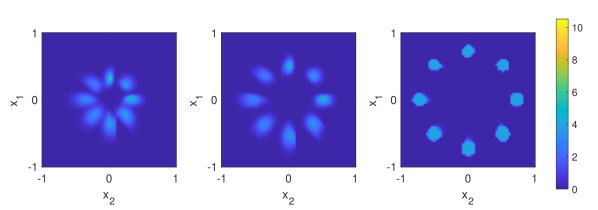
(b) Asymmetric kernel

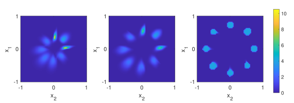
(c) Asymmetric kernel (coordination transform)

Fig. 1. MFG solution $\rho(x,0.3),\rho(x,0.6),\rho(x,1)$ for density splitting examples.

The results are shown in Figure 1. As we can see nonlocal kernel affect how the density moves and have different final distributions. In case A, a symmetric kernel leads to an even splitting of the initial density. Comparing case A and B, we see that the large $\delta_{1,-}$ causes density to favor a motion towards $x_{1,-}$ direction. As a result, the final density has more concentration in $x_{1,-}$ domain. As for a comparison between A and C, we see that agents in case C have a preference to move along $x_{1}=x_{2}$ direction, which is consistent with the shape of the kernel $K(x,0)$.

5.2. Static Obstacles Modeled with Density constraint

Here we provide a MFG problem where the the density moves while avoiding the obstacles, which is modeled using density constraint. We also include a small local interaction term in this example:

$$\begin{split}&f_{0}(t,x,z)=\partial_{z}\mathbf{1}_{\underline{h}(x,t)\leq z\leq\bar{h}(x,t)}+\epsilon\log{z},\quad\epsilon=0.01,\\ &\bar{h}(x,t)=0,\bar{e}(x)=0\;\text{for}\;x\in\Omega_{obs},\\ &K(x,y)=4\gamma_{\delta_{-},\delta}(x_{1}-y_{1})\gamma_{\delta,\delta}(x_{2}-y_{2}),\quad\delta=0.1,\delta_{-}=0.4\end{split}$$

As for the initial-terminal conditions, we have

$$\begin{split}&\rho_{0}(x)=\frac{1}{2}\mathcal{N}([-0.8,0.5],0.1)+\frac{1}{2}\mathcal{N}([-0.8,0.5],0.1)\\ &g(x)=x_{1}^{2}+\left(x_{2}-0.85\right)^{2}-2e^{-10\left(x_{2}-0.75\right)^{2}}.\end{split}$$

Under above setup, we consider the following $2$ cases: case A, $\bar{h}(x,t)=20$; case B, $\bar{h}(x,t)=10$ for all $(x,t),x\notin\Omega_{obs}$.

(a) $\bar{h}(x,t)=20$

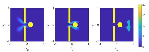
(b) $\bar{h}(x,t)=10$

Fig. 2. MFG solution $\rho(x,0.3),\rho(x,0.6),\rho(x,1)$ for static obstacles examples, where the obstacle (yellow) is located at $\Omega_{obs}=\left\{\|x-[0,0.2]\|^{2}\leq 0.15^{2}\right\}\cup\left\{|x_{1}|\geq 0.1,|x_{2}+0.15|\leq 0.05\right\}$

The numerical results are shown in Figure 2. As we see the density moves from left to the right and avoids both the rectangle and round obstacles. It avoids the round obstacles via an uneven splitting, which is caused by the asymmetric kernel. Comparing Case A and B, we see that the density constraint make the agents spread more.

5.3. Dynamic Obstacles Modeled with Density constraint

In the last example, we model an Optimal-Transport-like problem with dynamic obstacles via density constraint. Our mean field game system is as follows:

$$\begin{split}&K(x,y)=\exp\left(-\frac{\|x-y\|^{2}}{2\delta^{2}}\right),\quad\delta=0.1\\ &\rho_{0}(x)=\sum_{j=1}^{5}\frac{1}{5}\mathcal{N}(x_{j},0.05),\text{for}\;x_{j}=[-0.9+0.3j,-0.85]\\ &g(x)=x_{1}^{2}+5|x_{2}-0.85|^{1.5}.\end{split}$$

We use the density constraint $\bar{h}(x,t)$ to model 4 rectangles moving vertically. As for the density constraint at final time, we choose $\underline{e}(x)$ to be exactly a density distribution. Specifically,

$$\underline{e}(x)=c_{e},\;\text{for}\;\|x-x_{j}\|\leq 0.08,\;\text{for}\;x_{j}=[-0.9+0.3j,0.85],j=1...5,$$

where $c_{e}$ is a constant that normalized $\underline{e}(x)$. This setup is equivalent to specifying the final density distribution $\rho(x,1)=\underline{e}(x)$. This is case A that is shown in Figure 3.

(a) $\underline{e}(x)=c_{e}$

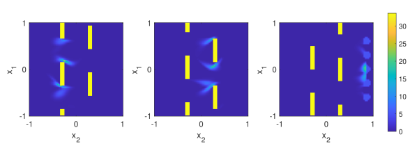
(b) $\underline{e}(x)=\frac{1}{2}c_{e}$

Fig. 3. MFG solution $\rho(x,0.3),\rho(x,0.6),\rho(x,1)$ for dynamic obstacles examples.

We also relax the density constraint at $t=1$, by setting

$$\underline{e}(x)=\frac{1}{2}c_{e},\;\text{for}\;\|x-x_{j}\|\leq 0.08,\;\text{for}\;x_{j}=[-0.9+0.3j,0.85],j=1...5.$$

That it, we decrease the lower bound of $\rho(x,1)$ by half. This is Case B shown in Figure 3. As we can see, unlike case A, the agents do not completely fill the support of $\underline{e}(x)$. The aspect of modeling dynamic obstacles also works well as agents avoid the prohibited regions.

Appendix

Proof of Proposition 2.1

Calculating the first variation with respect to $\rho,m$ in (2.6), we obtain

$$\begin{cases}L\left(t,x,\frac{m}{\rho}\right)-\frac{m}{\rho}\nabla_{v}L\left(t,x,\frac{m}{\rho}\right)+\alpha(x,t)+\sum_{i=1}^{r}a_{i}(t)\zeta_{i}(x)+\phi_{t}=0\\ \nabla_{v}L\left(t,x,\frac{m}{\rho}\right)+\nabla\phi=0\\ \beta(x)+\sum_{i=1}^{r}b_{i}\zeta_{i}(x)-\phi(x,1)=0\\ \end{cases}$$

Additionally, $\rho(x,0)=\rho_{0}(x)$ as $\Xi(\rho,m)<\infty$. From the properties of the Legendre transform, we obtain that

$$\begin{cases}\frac{m}{\rho}=-\nabla_{p}H(t,x,\nabla\phi)\\ H(t,x,\nabla\phi)=\frac{m}{\rho}\nabla_{v}L\left(t,x,\frac{m}{\rho}\right)-L\left(t,x,\frac{m}{\rho}\right)\end{cases}$$

which yields (2.4). Rest of the proof readily follows from the convex duality relation between $\Xi$ and $\Xi^{*}$.

Proof of Proposition 2.2

The components of $C^{*}$ corresponding to variables $a,b,\alpha,\beta$ are straightforward to calculate as they are in $L^{2}$ spaces. As for the component corresponding to $\phi$, we have to find $h=h(\rho,m)$ such that for all $\phi$ one has that

$$\begin{split}\langle h,\phi\rangle_{H^{1}}=&-\int_{0}^{1}\int_{\Omega}\phi_{t}\rho+\nabla\phi\cdot mdxdt+\int_{\Omega}\phi(x,1)\rho(x,1)dx-\int_{\Omega}\phi(x,0)\rho(x,0)dx\\ =&\int_{0}^{1}\int_{\Omega}\phi\left(\rho_{t}+\nabla\cdot m\right)dxdt\end{split}$$

We have that

$$\begin{split}{\langle}h,\phi{\rangle}_{H^{1}}=&\int_{\Omega}\phi(x,0)h(x,0)dx+\int_{\Omega}\phi(x,1)h(x,1)dx+\int_{0}^{1}\int_{\Omega}\nabla_{t,x}\phi\cdot\nabla_{t,x}hdxdt\\ =&-\int_{0}^{1}\int_{\Omega}\phi\Delta_{t,x}hdxdt+\int_{\Omega}\phi(x,1)\left(h(x,1)+h_{t}(x,1)\right)dx\\ &+\int_{\Omega}\phi(x,0)\left(h(x,0)-h_{t}(x,0)\right)dx\end{split}$$

Therefore $h$ must satisfy the conditions

$$\begin{cases}\Delta_{t,x}h=-\left(\rho_{t}+\nabla\cdot m\right)\\ h(x,0)-h_{t}(x,0)=0\\ h(x,1)+h_{t}(x,1)=0\end{cases}$$ (5.1)

and we obtain (2.14). Next, we prove (2.15). We have that

$$U_{0}^{*}(\alpha)=\int_{0}^{1}\int_{\Omega}F_{0}^{*}(t,x,\alpha(x,t))dxdt,\quad\partial_{\alpha}U_{0}^{*}(\alpha(x,t))=\partial_{\alpha}F_{0}^{*}(t,x,\alpha(x,t)),$$

where $F_{0}^{*}(t,x,\alpha)=\sup_{\rho}\alpha\rho-F_{0}(t,x,\rho)$. Therefore, the $\alpha$-entry inclusion in (2.15) is equivalent to

$$\rho(x,t)\in\partial_{\alpha}F_{0}^{*}(t,x,\alpha(x,t))\Longleftrightarrow\alpha(x,t)\in\partial_{\rho}F_{0}(t,x,\rho)=f_{0}(t,x,\rho)$$

Similarly, the $\beta$-entry inclusion is equivalent to

$$\rho(x,1)\in\partial_{\alpha}G_{0}^{*}(x,\beta(x))\Longleftrightarrow\beta(x)\in\partial_{\rho}G_{0}(x,\rho(x,1))=g_{0}(x,\rho(x,1))$$

Next, the $\phi$-entry inclusion means that $h=0$ in (5.1) that is equivalent to

$$\rho_{t}+\nabla\cdot m=0$$

The $a$-entry inclusion in (2.15) is

$$\left(\int_{\Omega}\rho(x,t)\zeta_{i}(x)dx\right)_{i=1}^{r}\in\mathbf{K}^{-1}\partial_{a}U_{1}^{*}(a)\Longleftrightarrow\mathbf{K}\left(\int_{\Omega}\rho(x,t)\zeta_{i}(x)dx\right)_{i=1}^{r}\in\partial_{a}U_{1}^{*}(a)$$

Applying the properties of the Legendre transform again, we obtain that this previous inclusion is equivalent to

$$a\in\partial_{c}U_{1}\left(\mathbf{K}\left(\int_{\Omega}\rho(x,t)\zeta_{i}(x)\right)_{i=1}^{r}\right)$$ (5.2)

On the other hand, we have that

$$\begin{split}\partial_{c_{i}}U_{1}(c)=\int_{0}^{1}\int_{\Omega}f_{1}\left(t,x,\sum_{p=1}^{r}c_{p}(t)\zeta_{p}(x)\right)\zeta_{i}(x)dxdt\end{split}$$

and therefore

$$\begin{split}&\partial_{c_{i}}U_{1}\left(\mathbf{K}\left(\rho(x,t)\zeta_{i}(x)\right)_{i=1}^{r}\right)\\ =&\int_{0}^{1}\int_{\Omega}f_{1}\left(t,x,\sum_{p=1}^{r}\sum_{q=1}^{r}k_{pq}\int_{\Omega}\rho(y,t)\zeta_{q}(y)dy\zeta_{p}(x)\right)\zeta_{i}(x)dxdt\\ =&\int_{0}^{1}\int_{\Omega}f_{1}\left(t,x,\int_{\Omega}K_{r}(x,y)\rho(y,t)dy\right)\zeta_{i}(x)dxdt\end{split}$$

Hence, (5.2) is equivalent to the first equation in (2.5). The derivation for the $b$-entry in (2.15) is similar.

Proof of Theorem 2.4

The equivalence of (2.17) and (2.4)-(2.5) is simply a combination of assertions in Propositions 2.1 and 2.2. Furthermore, assume that $c\mapsto\partial_{c}U_{1}(\mathbf{K}c)$ and $w\mapsto\partial_{w}V_{1}(\mathbf{S}w)$ are maximally monotone. We have that

$$\left(\partial_{c}U_{1}\left(\mathbf{K}c\right)\right)^{-1}=\mathbf{K}^{-1}\partial_{a}U_{1}^{*}(a),\quad\left(\partial_{w}V_{1}\left(\mathbf{S}w\right)\right)^{-1}=\mathbf{S}^{-1}\partial_{b}V_{1}^{*}(b)$$

Therefore $a\mapsto\mathbf{K}^{-1}\partial_{a}U_{1}^{*}(a)$ and $b\mapsto\mathbf{S}^{-1}\partial_{b}V_{1}^{*}(b)$ are maximally monotone. Next, $\alpha\mapsto\partial_{\alpha}U_{0}^{*}(\alpha)$ and $\beta\mapsto\partial_{\beta}V_{0}^{*}(\beta)$ are maximally monotone by the convexity of $U_{0}^{*},V_{0}^{*}$. Hence, $M$ is maximally monotone.

References

• [1] Yves Achdou. Finite difference methods for mean field games. In Hamilton-Jacobi equations: approximations, numerical analysis and applications, volume 2074 of Lecture Notes in Math., pages 1–47. Springer, Heidelberg, 2013.
• [2] Yves Achdou, Fabio Camilli, and Italo Capuzzo-Dolcetta. Mean field games: convergence of a finite difference method. SIAM J. Numer. Anal., 51(5):2585–2612, 2013.
• [3] Yves Achdou and Italo Capuzzo-Dolcetta. Mean field games: numerical methods. SIAM J. Numer. Anal., 48(3):1136–1162, 2010.
• [4] Noha Almulla, Rita Ferreira, and Diogo Gomes. Two numerical approaches to stationary mean-field games. Dyn. Games Appl., 7(4):657–682, 2017.
• [5] J.-D. Benamou and G. Carlier. Augmented Lagrangian methods for transport optimization, mean field games and degenerate elliptic equations. J. Optim. Theory Appl., 167(1):1–26, 2015.
• [6] J.-D. Benamou, G. Carlier, and F. Santambrogio. Variational mean field games. In Active particles. Vol. 1. Advances in theory, models, and applications, Model. Simul. Sci. Eng. Technol., pages 141–171. Birkhäuser/Springer, Cham, 2017.
• [7] L. Briceño Arias, D. Kalise, Z. Kobeissi, M. Laurière, Á. Mateos González, and F. J. Silva. On the implementation of a primal-dual algorithm for second order time-dependent mean field games with local couplings. In CEMRACS 2017—numerical methods for stochastic models: control, uncertainty quantification, mean-field, volume 65 of ESAIM Proc. Surveys, pages 330–348. EDP Sci., Les Ulis, 2019.
• [8] L. M. Briceño Arias, D. Kalise, and F. J. Silva. Proximal methods for stationary mean field games with local couplings. SIAM J. Control Optim., 56(2):801–836, 2018.
• [9] Fabio Camilli and Francisco Silva. A semi-discrete approximation for a first order mean field game problem. Netw. Heterog. Media, 7(2):263–277, 2012.
• [10] P. Cardaliaguet. Notes on mean field games, 2013. https://www.ceremade.dauphine.fr/ cardaliaguet/.
• [11] Pierre Cardaliaguet and Saeed Hadikhanloo. Learning in mean field games: the fictitious play. ESAIM Control Optim. Calc. Var., 23(2):569–591, 2017.
• [12] E. Carlini and F. J. Silva. A fully discrete semi-Lagrangian scheme for a first order mean field game problem. SIAM J. Numer. Anal., 52(1):45–67, 2014.
• [13] Elisabetta Carlini and Francisco J. Silva. A semi-Lagrangian scheme for a degenerate second order mean field game system. Discrete Contin. Dyn. Syst., 35(9):4269–4292, 2015.
• [14] Elisabetta Carlini and Francisco J. Silva. On the discretization of some nonlinear fokker–planck–kolmogorov equations and applications. SIAM Journal on Numerical Analysis, 56(4):2148–2177, 2018.
• [15] Antonin Chambolle and Thomas Pock. A first-order primal-dual algorithm for convex problems with applications to imaging. J. Math. Imaging Vision, 40(1):120–145, 2011.
• [16] Antonin Chambolle and Thomas Pock. On the ergodic convergence rates of a first-order primal-dual algorithm. Math. Program., 159(1-2, Ser. A):253–287, 2016.
• [17] Diogo A. Gomes and J. Saúde. Mean field games models—a brief survey. Dyn. Games Appl., 4(2):110–154, 2014.
• [18] Diogo A. Gomes and João Saúde. Numerical methods for finite-state mean-field games satisfying a monotonicity condition. Applied Mathematics & Optimization, 2018.
• [19] P. Jameson Graber and Alpár R. Mészáros. Sobolev regularity for first order mean field games. Ann. Inst. H. Poincaré Anal. Non Linéaire, 35(6):1557–1576, 2018.
• [20] Olivier Guéant, Jean-Michel Lasry, and Pierre-Louis Lions. Mean field games and applications. In Paris-Princeton Lectures on Mathematical Finance 2010, volume 2003 of Lecture Notes in Math., pages 205–266. Springer, Berlin, 2011.
• [21] Saeed Hadikhanloo. Learning in anonymous nonatomic games with applications to first-order mean field games. arXiv: Optimization and Control, 2017.
• [22] Saeed Hadikhanloo and Francisco J. Silva. Finite mean field games: fictitious play and convergence to a first order continuous mean field game. J. Math. Pures Appl. (9), 132:369–397, 2019.
• [23] M. Huang, P. E. Caines, and R. P. Malhamé. Large-population cost-coupled LQG problems with nonuniform agents: individual-mass behavior and decentralized $\epsilon$-Nash equilibria. IEEE Trans. Automat. Control, 52(9):1560–1571, 2007.
• [24] M. Huang, R. P. Malhamé, and P. E. Caines. Large population stochastic dynamic games: closed-loop McKean-Vlasov systems and the Nash certainty equivalence principle. Commun. Inf. Syst., 6(3):221–251, 2006.
• [25] M. Jacobs and F. Léger. A fast approach to optimal transport: the back-and-forth method. Preprint, 2019. arXiv:1905.12154 [math.OC].
• [26] Matt Jacobs, Flavien Léger, Wuchen Li, and Stanley Osher. Solving large-scale optimization problems with a convergence rate independent of grid size. SIAM J. Numer. Anal., 57(3):1100–1123, 2019.
• [27] Jean-Michel Lasry and Pierre-Louis Lions. Jeux à champ moyen. I. Le cas stationnaire. C. R. Math. Acad. Sci. Paris, 343(9):619–625, 2006.
• [28] Jean-Michel Lasry and Pierre-Louis Lions. Jeux à champ moyen. II. Horizon fini et contrôle optimal. C. R. Math. Acad. Sci. Paris, 343(10):679–684, 2006.
• [29] Jean-Michel Lasry and Pierre-Louis Lions. Mean field games. Jpn. J. Math., 2(1):229–260, 2007.
• [30] Siting Liu, Matthew Jacobs, Wuchen Li, Levon Nurbekyan, and Stanley J. Osher. Computational methods for nonlocal mean field games with applications, 2020.
• [31] Levon Nurbekyan. One-dimensional, non-local, first-order stationary mean-field games with congestion: a Fourier approach. Discrete Contin. Dyn. Syst. Ser. S, 11(5):963–990, 2018.
• [32] Levon Nurbekyan and J. Saúde. Fourier approximation methods for first-order nonlocal mean-field games. Port. Math., 75(3-4):367–396, 2018.
• [33] Bang Công Vũ. A variable metric extension of the forward-backward-forward algorithm for monotone operators. Numer. Funct. Anal. Optim., 34(9):1050–1065, 2013.