Efficient parallel 3D computation of the compressible Euler equations with an invariant-domain preserving second-order finite-element scheme

Abstract.

We discuss the efficient implementation of a high-performance second-order collocation-type finite-element scheme for solving the compressible Euler equations of gas dynamics on unstructured meshes. The solver is based on the convex limiting technique introduced by Guermond et al. (SIAM J. Sci. Comput. 40, A3211–A3239, 2018). As such it is invariant-domain preserving, i. e., the solver maintains important physical invariants and is guaranteed to be stable without the use of ad-hoc tuning parameters. This stability comes at the expense of a significantly more involved algorithmic structure that renders conventional high-performance discretizations challenging. We develop an algorithmic design that allows SIMD vectorization of the compute kernel, identify the main ingredients for a good node-level performance, and report excellent weak and strong scaling of a hybrid thread/MPI parallelization.

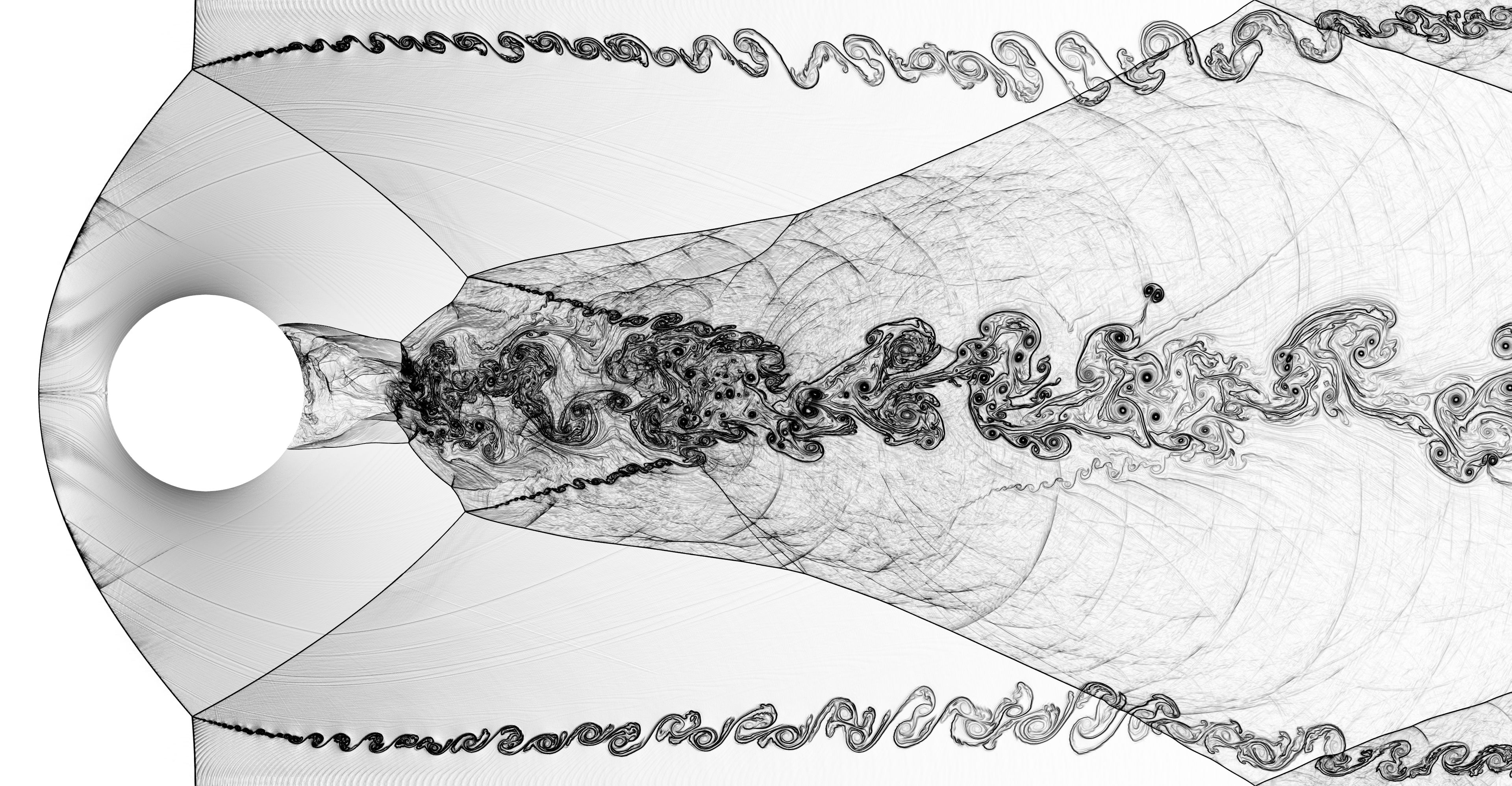
Figure 1. 2D Mach 3 compressible Euler flow around a disc; 38 M unstructured $\mathcal{Q}_{1}$ nodes, Schlieren-like plot at $t=3.5$.

figure description

1. Introduction

The appropriate discretization and simulation of the compressible Euler equations of gas dynamics is an ongoing and intensely discussed debate (Zalesak, 2005; Kuzmin and Möller, 2005; Barlow et al., 2016; Guermond et al., 2018). This is in contrast to, for example, the incompressible Navier-Stokes equations for which a much more complete mathematical solution theory is available that establishes a common framework to assess the quality and approximation property of fluid solvers at least for the pre-turbulent regime (Schäfer et al., 1996). The lack of an accepted solution theory for the Euler equations allows for considerable freedom in the the notion what constitutes a good computational approximation (see for example (Zalesak, 2005; Kuzmin and Möller, 2005)) and thus in the choice of discretization scheme. Consequently, discretization schemes that allow for a high arithmetic intensity and good parallel scaling have received a high level of attention during the last decade. An important example are high-order discontinuous Galerkin (DG) discretizations (Wang et al., 2013; Witherden et al., 2014; Kronbichler and Kormann, 2019) with some form of flux reconstruction and appropriate flux/slope limiters (Cockburn and Shu, 1989). However, in the transonic and supersonic regime found in certain shock-hydrodynamics applications, the use of variational schemes might become questionable due to the lack of pointwise stability properties—at least without the perpetual hunt for the right shock capturing technique (Barlow et al., 2016).

In this publication we want to entertain a different approach. Instead of starting with a high-order discretization and then constructing ad-hoc limiting techniques for solving certain benchmark problems, we instead start with the mathematical description of a second-order collocation-type finite-element scheme that is based on the convex-limiting technique pioneered by Guermond et al. (Guermond and Popov, 2016b, a, 2017; Guermond et al., 2018). The methodology is invariant-domain preserving (Guermond and Popov, 2017). This means that in addition to the usual notion of hyperbolic conservation (regarding density, momentum and total energy), a number of important physical invariance principles are maintained strongly: positivity of the density and internal energy and a local minimum principle on the specific entropy (see Section 3.9). The method is guaranteed to be stable without the use of any ad-hoc tuning parameters. This stability comes at the expense of a significantly more involved algorithmic structure. Taking the mathematical properties of the convex-limited collocation-type continuous Galerkin scheme as a given, the contribution of the present work is the identification of data structures and algorithms that make it run fast on modern hardware, and characterize the proposed computing kernels in an academic setting. In detail, our contributions with the current work can be summarized as follows:

• We describe the algorithmic structure of a second-order collocation-type finite-element scheme for solving the compressible Euler equations of gas dynamics. Our solver is based on a slight modification of (Guermond et al., 2018) suitable for SIMD vectorization to render it highly process and thread parallelizable. A high degree of instruction-level vectorization can be achieved for a nonlinear convex-limiting scheme that involves a large number of root-finding problems with transcendental functions as building blocks. Our approach is based on explicit vectorization using the C++ template mechanism and operator overloading as a high-level user interface (Arndt et al., 2021; Kronbichler and Kormann, 2012), as well as on algorithmic design that avoids branching on data.

• We comment on optimization strategies to achieve excellent scaling characteristics and absolute performance, such as, avoiding index translations, cache-optimized traversal of data structures, using point-to-point MPI communication, and efficient local caching. To this end we introduce a SIMD-optimized sparsity pattern that uses a hybrid storage format blending a packed row (ELL) format for highly structures SIMD parallel regions with a more flexible compressed sparse row (CSR) storage format for non-vectorized index regions.

• We report excellent weak and strong scaling of our implementation for both 2D and 3D problems, and demonstrate that our solver is able to tackle realistic 3D applications by computing a flow problem in 3D with about 1.8 billion gridpoints (totalling to about 8 billion spatial degrees of freedom).

• The main performance limitations of the solver are assessed, considering the mathematical model as fixed down to roundoff precision. Our analysis identifies which mathematical steps could be modified to further improve performance in the future. This analysis gives a guideline for performance optimization of a broader class of algorithms based on unstructured-grid stencil-based update formulas with complex data dependencies and heavy transcendental arithmetic. In addition, the analysis allows for predictions regarding the expected performance envelope on hardware with different characteristics than the present CPU-based architectures.

• A reference implementation of the solver is made available that is based on the deal.II finite element library (Arndt et al., 2019; Arndt et al., 2021) and is freely available for the scientific community under an open source license.

The remainder of the paper is organized as follows. In Section 2 we review the compressible Euler equations and introduce important physical quantities. In Section 3 the solver is discussed in a concise, abstract (mathematical) manner. In particular, the invariant domain property of the solver is discussed in Section 3.3 and the convex limiting paradigm is introduced in Section 3.4. We summarize key design decisions of our implementation in Section 4 and report benchmark results and explore algorithmic alternatives in Section 5. We conclude in Section 6 with a detailed discussion of possible further improvements that require some mathematical reformulation.

2. The Euler equations of gas dynamics

Let $\Omega$ be an open polyhedral domain in ${\mathbb{R}}^{d}$, $d=1,2,3$. We consider the compressible Euler equations in conservative form,

(1) $$\partial_{t}{\boldsymbol{u}}\,+\,\nabla\cdot\,{\mathbbm{f}}({\boldsymbol{u}})=0,$$

equipped with suitable initial conditions ${\boldsymbol{u}}({\boldsymbol{x}},0)={\boldsymbol{u}}_{0}$. Here, the independent variables are $({\boldsymbol{x}},t)\in\Omega\times{\mathbb{R}}_{+}$ and the vector ${\boldsymbol{u}}:=(\rho,{\boldsymbol{m}},E)^{\mathsf{T}}\in{\mathbb{R}}^{d+2}$ describes the (dependent) conserved quantities, the density $\rho$, the momentum ${\boldsymbol{m}}$, and the total energy $E$. The flux ${\mathbbm{f}}({\boldsymbol{u}})\in{\mathbb{R}}^{(d+2)\times d}$ is given by

(2) $${\mathbbm{f}}({\boldsymbol{u}}):=\begin{pmatrix}{\boldsymbol{m}}\;,\;{\boldsymbol{v}}\otimes{\boldsymbol{m}}+p{\mathbb{I}}_{d}\;,\;{\boldsymbol{v}}(E+p)\end{pmatrix}^{\mathsf{T}},$$

where ${\mathbb{I}}_{d}$ is the $d\times d$ identity matrix, and $p$ is the pressure that will be defined below. Starting from the vector ${\boldsymbol{u}}$ of conserved quantities we define a number of derived physical quantities. The velocity of the fluid particles is denoted ${\boldsymbol{v}}:=\rho^{-1}{\boldsymbol{m}}$ and $e:=\rho^{-1}E-\frac{1}{2}{\boldsymbol{v}}^{2}$ denotes the specific internal energy. We call the quantity $\varepsilon:=\rho e=E-\frac{1}{2}\rho{\boldsymbol{v}}^{2}$ internal energy. Here, we have used the notation ${\boldsymbol{v}}^{2}:=\|{\boldsymbol{v}}\|^{2}$, where $\|\cdot\|$ is the Euclidean norm.

The pressure $p$ is defined by an equation of state derived from a specific entropy $s(\rho,e)$ (Guermond and Popov, 2016b; Harten, 1983). For the sake of simplicity we limit the discussion in this paper to a polytropic ideal gas by setting

$$s(\rho,e)-s_{0}\;=\;\log\Big{(}e^{\frac{1}{\gamma-1}}\rho^{-1}\Big{)},$$

where $\gamma$ is the ratio of specific heats that we set to $\gamma=7\diagup 5$. This implies that

$$p\;:=\;-\rho^{2}\frac{{\mathrm{d}}s}{{\mathrm{d}}\rho}\Big{(}\frac{{\mathrm{d}}s}{{\mathrm{d}}e}\Big{)}^{-1}\;=\;(\gamma-1)\,\varepsilon.$$

We also introduce the speed of sound $c=\sqrt{\frac{\gamma\,p}{\rho}}$, as well as a scaled specific entropy that will be used in the context of convex limiting,

(3) $$\phi({\boldsymbol{u}})\;:=\;\exp\big{(}(\gamma-1)\,s(\rho,e({\boldsymbol{u}}))\big{)}\;=\;\varepsilon\,\rho^{-\gamma}.$$

As a last preparatory step we introduce a Harten-type entropy (Harten, 1983, Eq. 2.10a),

(4) $$\eta({\boldsymbol{u}})\;:=\;\big{(}\rho^{2}e\big{)}^{\frac{1}{\gamma+1}}\;=\;\big{(}\rho\varepsilon\big{)}^{\frac{1}{\gamma+1}}.$$

3. Second-order invariant-domain preserving Euler scheme

Before proceeding to the algorithmic details of our solver we summarize the method in this section in a concise, mathematical manner. Our solver is based on the convex-limiting technique pioneered by Guermond et al. (Guermond et al., 2018). We refer the reader to (Guermond and Popov, 2016b, a, 2017; Guermond et al., 2018) for a detailed derivation and analysis of the respective building blocks. We summarize and slightly adapt the algorithm here with the aim of developing a scalable hybrid-parallelized solver that can utilize modern hardware. In the following, we introduce the underlying finite-element discretization, low- and high-order update step, as well as necessary building blocks for the final time stepping (Section 3.5).

3.1. Finite element discretization

Let $\mathcal{T}_{h}$ be a partition of $\Omega$ into a shape-regular quadrilateral or hexahedral mesh. We denote by $\big{\{}\varphi_{i}^{h}\big{\}}_{i}^{\mathcal{N}}$ the Lagrange basis of $\mathbb{Q}_{1}(\mathcal{T}_{h})$, the space of piecewise linear, bilinear, or trilinear finite elements on $\Omega$ ($d=1$, $2$, $3$). In the following we will make use of two fundamental properties of the Lagrange basis, the nonnegativity of the lumped mass matrix and a partition of unity property, respectively,

$$\int_{\Omega}\varphi_{i}^{h}{\mathrm{d}}x>0\quad\text{for }\;1\leq i\leq\mathcal{N},\qquad\qquad\sum_{i=1}^{\mathcal{N}}\varphi_{i}^{h}(x)=1\quad\text{for }x\in\Omega.$$

Following the notation in (Guermond et al., 2018), we introduce a number of scalar and vector-valued matrix elements:

(5) $$\begin{drcases}\begin{aligned} m_{ij}&\coloneqq\int_{\Omega}\varphi^{h}_{i}(x)\varphi^{h}_{j}(x){\mathrm{d}}x,&\qquad\qquad m_{i}&\coloneqq\int_{\Omega}\varphi^{h}_{i}(x){\mathrm{d}}x,\qquad\\[3.00003pt] {\boldsymbol{c}}_{ij}&\coloneqq\int_{\Omega}\varphi^{h}_{i}(x)\nabla\varphi^{h}_{j}(x){\mathrm{d}}x,&\qquad\qquad{\boldsymbol{n}}_{ij}&\coloneqq\frac{{\boldsymbol{c}}_{ij}}{\|{\boldsymbol{c}}_{ij}\|},\qquad\\[3.00003pt] \beta_{ij}&\coloneqq\int_{\Omega}\nabla\varphi^{h}_{i}(x)\cdot\nabla\varphi^{h}_{j}(x){\mathrm{d}}x,&\qquad\qquad b_{ij}&\coloneqq\delta_{ij}-\frac{m_{ij}}{m_{j}},\end{aligned}\end{drcases}$$

where $\delta_{ij}$ denotes Kronecker’s delta. The matrices introduced in (5) only depend on the mesh and the particular choice of the finite element basis. For a given index $i$, we introduce a stencil of nonzero matrix entries

$$\mathcal{I}(i)\coloneqq\big{\{}1\leq j\leq\mathcal{N}\;\big{|}\;\text{supp}\,(\varphi_{i}^{h})\cap\text{supp}\,(\varphi_{j}^{h})\not=\emptyset\big{\}}.$$

3.2. Efficient precomputation

The solver algorithm discussed in the following consists of nonlinear updates that are organized as loops over the stencil:

for $i=1$, …, $\mathcal{N}$ do

       for $j\in\mathcal{I}(i)$ do

             (Nonlinear) computation involving quantities with indices $i$ and $j$

      

This is a stencil-centric operation in contrast to the usual cell-centric loops typically encountered in finite element assembly (Arndt et al., 2021). In order to achieve good performance, the first decision is whether the matrices defined in (5) should be recomputed “on the fly” in terms of a matrix-free approach, or whether it is more efficient to precompute and store some matrices. For low-order discretizations, matrix-free schemes based on fast integration with sum factorization cannot amortize the work at quadrature points to a sufficient number of degrees of freedom (dofs) on a cell, thus incurring a substantial arithmetic overhead compared to matrix-based schemes (Fischer et al., 2020; Kronbichler and Kormann, 2012, 2019). The overhead is around 500 floating point operations per nonzero entry for tri-linear polynomials in 3D using similar arguments as for the operator action in (Kronbichler and Kormann, 2012, Fig. 1). These computations are necessary because some of the nonlinear update steps specified below explicitly require the full value of the $(i,j)$-th entry of the respective matrix. We point out that even hierarchical, stencil-based matrix-free methods (such as (Bergen et al., 2006)) will need to incorporate additional steps to treat nonlinearities or deformed meshes (we refer to (Bauer et al., 2018) for a possible approach). As will be shown below, many steps are below the threshold of saturating memory bandwidth in a matrix-based implementation for contemporary hardware. Furthermore, a reformulation of our algorithms in terms of a cell-based loop, viz.

for $T\in\mathcal{T}_{h}$ do

       for $i$ with $\text{supp}\,\big{(}\varphi^{h}_{i}\big{)}\cap T\not=\emptyset$ do

             for $j$ with $\text{supp}\,\big{(}\varphi^{h}_{j}\big{)}\cap T\not=\emptyset$ do

                   …A

            

      

would necessitate additional communication from degrees of freedom from different cells, which is better done before the time loop. Based on these considerations, the limiting resource identification underlying the roofline performance model (Williams et al., 2009) suggests that the on-the-fly matrix-free computation would not relax the performance-limiting factor. Even though arithmetic intensity would be further increased, the application metric of the throughput in terms of points updated per second would decrease. Consequently, the most performance-beneficial setup is a stencil-based loop structure with pre-computed matrices.

Starting from these considerations, we avoid all assembly operations during the time loop and precompute the three matrices $m_{ij}$, ${\boldsymbol{c}}_{ij}$, $\beta_{ij}$. Note that each matrix contains unique information in terms of the shape functions. Furthermore, the frequent use of the diagonal matrix $m_{i}\delta_{ij}$ on the one hand and the low memory consumption on the other motivates to also store this matrix. Given one layer of overlap in the mesh to the neighboring MPI ranks, the computation of those four matrices is completely local to each MPI rank. Conversely, the matrices ${\boldsymbol{n}}_{ij}$ and $b_{ij}$ are derived on the fly from ${\boldsymbol{c}}_{ij}$ and $m_{ij}$: Matrix ${\boldsymbol{n}}_{ij}$ is used in close proximity to ${\boldsymbol{c}}_{ij}$, thus leading to a single division and three multiplications of data present already in registers, which is cheaper than transferring three doubles through the memory hierarchy. The motivation for $b_{ij}$ is more subtle: The code below uses both $b_{ij}$ and $b_{ji}$ for the update; whereas $m_{ij}$ is symmetric, the matrix $b_{ij}$ is not. In the presence of caches, see the analysis below, it is hence cheaper to only load the symmetric entry $m_{ij}$ and the entries $1/m_{i}$ and $1/m_{j}$ derived from the diagonal mass matrix. In addition, we propose to precompute the inverse of the lumped mass matrix, $(1/m_{i}\,\delta_{ij})$, in order to avoid divisions. We refer to the detailed discussion in Section 5.

3.3. Intermediate low-order update

Given a snapshot $\big{(}{\boldsymbol{U}}_{i}^{n}\big{)}_{1\leq i\leq\mathcal{N}}$ of admissible states at time $t_{n}$ (this is to say that $\rho({\boldsymbol{U}}_{i}^{n})>0$ and $\varepsilon({\boldsymbol{U}}_{i}^{n})>0$ ) with an associated finite-element function ${\boldsymbol{u}}_{h}^{n}=\sum_{i=1}^{\mathcal{N}}{\boldsymbol{U}}_{i}^{n}\varphi^{h}_{i}$, our goal is to compute a new snapshot $\big{(}{\boldsymbol{U}}_{i}^{n+1}\big{)}_{1\leq i\leq\mathcal{N}}$ consistent with the Euler equations (1) such that the states maintain the following crucial thermodynamical constraints

• admissibility: positivity of density, $\rho({\boldsymbol{U}}_{i}^{n+1})>0$, and positivity of internal energy, $\varepsilon({\boldsymbol{U}}_{i}^{n+1})>0$,

• local minimum principle on specific entropy: $s({\boldsymbol{U}}_{i}^{n+1})\geq\min_{j\in\mathcal{I}(i)}\,s(U_{j}^{n})$.

The first algorithmic ingredient to achieve a high-order update obeying above constraints is the computation of an intermediate low-order update ${\boldsymbol{U}}_{i}^{L,n+1}$ with a first-order graph viscosity method (Guermond and Popov, 2016b). The method is based on a guaranteed maximum wavespeed estimate coming from an approximate Riemann solver (Guermond and Popov, 2016a). We construct an explicit update of the state $u_{h}^{n}=\sum_{i=1}^{\mathcal{N}}{\boldsymbol{U}}_{i}^{n}\varphi^{h}_{i}$ at time $t_{n}$ for some new time $t_{n+1}=t_{n}+\tau_{n}$ as follows:

(6) $${\boldsymbol{U}}_{i}^{L,n+1}={\boldsymbol{U}}_{i}^{n}+\frac{\tau_{n}}{m_{i}}\sum_{j\in\mathcal{I}(i)}\Big{(}-{\mathbbm{f}}({\boldsymbol{U}}^{n}_{j})\cdot{\boldsymbol{c}}_{ij}+d_{ij}^{L,n}\big{(}{\boldsymbol{U}}^{n}_{j}-{\boldsymbol{U}}^{n}_{i}\big{)}\Big{)}.$$

Here, $d_{ij}^{L,n}$ is a graph viscosity given by

(7) $$d_{ij}^{L,n}\;\coloneqq\;\max\,\Big{(}\tilde{\lambda}_{\max}({\boldsymbol{n}}_{ij},{\boldsymbol{U}}^{n}_{i},{\boldsymbol{U}}^{n}_{j})\,|{\boldsymbol{c}}_{ij}|\,,\,\tilde{\lambda}_{\max}({\boldsymbol{n}}_{ji},{\boldsymbol{U}}^{n}_{j},{\boldsymbol{U}}^{n}_{i})\,|{\boldsymbol{c}}_{ji}|\Big{)}\quad\text{for }i\not=j,\qquad d_{ii}^{L,n}=-\sum_{i\not=j\in\mathcal{I}(i)}d_{ij}^{L,n},$$

where $\tilde{\lambda}_{\max}({\boldsymbol{n}}_{ij},{\boldsymbol{U}}^{n}_{i},{\boldsymbol{U}}^{n}_{j})$ is a suitable upper bound on the maximum wave speed in an associated one dimensional Riemann problem (Guermond and Popov, 2016b, a). The exact definition of $\tilde{\lambda}_{\max}({\boldsymbol{n}}_{ij},{\boldsymbol{U}}^{n}_{i},{\boldsymbol{U}}^{n}_{j})$ and description of the approximate Riemann solver that is used in the computation is postponed to Section 3.7. The time-step size is set to

(8) $$\tau_{n}=c_{\text{cfl}}\,\min_{1\leq i\leq\mathcal{N}}\left(\frac{m_{i}}{-2\,d_{ii}^{L,n}}\right),$$

with a chosen constant $0<c_{\text{cfl}}\leq 1$. In preparation for the high-order update with convex limiting, we rewrite the low-order update (6) as follows,

(9) $${\boldsymbol{U}}_{i}^{L,n+1}={\boldsymbol{U}}_{i}^{L,n}+\frac{2\,\tau_{n}}{m_{i}}\sum_{j\in\mathcal{I}(i)}d_{ij}^{L,n}\overline{{\boldsymbol{U}}}^{n}_{ij},\qquad\overline{{\boldsymbol{U}}}^{n}_{ij}\;\coloneqq\;\frac{1}{2}\big{(}{\boldsymbol{U}}^{n}_{i}+{\boldsymbol{U}}^{n}_{j}\big{)}-\frac{1}{2\,d_{ij}^{L,n}}\big{(}{\mathbbm{f}}({\boldsymbol{U}}^{n}_{j})-{\mathbbm{f}}({\boldsymbol{U}}^{n}_{i})\big{)}\cdot{\boldsymbol{c}}_{ij},$$

where we have used the identities $\sum_{j\in\mathcal{I}(i)}{\boldsymbol{c}}_{ij}={\boldsymbol{0}}$, and $\sum_{j\in\mathcal{I}(i)}d^{L,n}_{ij}=0$.

3.4. Intermediate high-order update

We now introduce a formally high-order update that is entropy consistent and close to being invariant-domain preserving (Guermond et al., 2018). The update is similar to the low-order update (6), the only difference being that the graph viscosity $d_{ij}^{L}$ of the low-order update is replaced by a suitable $d_{ij}^{H}\leq d_{ij}^{L}$ and the consistent mass matrix $m_{ij}$ is used instead of the lumped mass matrix $m_{i}$,

(10) $$\sum_{j\in\mathcal{I}(i)}m_{ij}\big{(}\tilde{\boldsymbol{U}}_{j}^{H,n+1}-{\boldsymbol{U}}_{j}^{n}\big{)}\;=\;\tau_{n}\sum_{j\in\mathcal{I}(i)}\Big{(}-{\mathbbm{f}}({\boldsymbol{U}}^{n}_{j})\cdot{\boldsymbol{c}}_{ij}+d_{ij}^{H,n}\big{(}{\boldsymbol{U}}^{n}_{j}-{\boldsymbol{U}}^{n}_{i}\big{)}\Big{)},$$

and where we set

(11) $$d_{ij}^{H,n}\;\coloneqq\;d_{ij}^{L,n}\,\frac{\alpha_{i}^{n}+\alpha_{j}^{n}}{2}\quad\text{for }i\not=j,\qquad d_{ii}^{H,n}=-\sum_{i\not=j\in\mathcal{I}(i)}d_{ij}^{H,n}.$$

Here, $\alpha_{i}^{n}$ denotes an indicator given by a normalized entropy viscosity ratio. The precise definition and computation of $\alpha_{i}^{n}$ is discussed in Section 3.8. Solving for $\tilde{\boldsymbol{U}}_{j}^{H,n+1}$ given by (10) involves inverting the full mass matrix. This is undesirable due to the high computational cost it incurs. Even with a competitive preconditioner, solving (10) can be as expensive as the entire rest of the full (explicit) update step. We avoid this issue and obtain a very efficient scheme by approximating the inverse of the matrix with a Neumann series. This introduces a second-order consistency error, which is however close to the underlying discretization error and much smaller than the error caused by the lumped mass matrix. We start by rewriting (10) as follows

(12) $$\sum_{j\in\mathcal{I}(i)}\frac{m_{ij}}{m_{j}}\;\frac{m_{j}}{\tau_{n}}\big{(}\tilde{\boldsymbol{U}}_{j}^{H,n+1}-{\boldsymbol{U}}_{j}^{n}\big{)}\;=\;{\boldsymbol{R}}^{n}_{i},\qquad\text{with}\quad{\boldsymbol{R}}^{n}_{i}\;\coloneqq\;\sum_{j\in\mathcal{I}(i)}\Big{(}-{\mathbbm{f}}({\boldsymbol{U}}^{n}_{j})\cdot{\boldsymbol{c}}_{ij}+d_{ij}^{H,n}\big{(}{\boldsymbol{U}}^{n}_{j}-{\boldsymbol{U}}^{n}_{i}\big{)}\Big{)}.$$

By expanding the inverse of the matrix $m_{ij}/m_{j}$ into a Neumann series up to first order,

$$\Big{(}\frac{m_{ij}}{m_{j}}\Big{)}^{-1}\,=\,\Big{(}\delta_{ij}-\big{(}\delta_{ij}-\frac{m_{ij}}{m_{j}}\big{)}\Big{)}^{-1}\;\approx\;\;\delta_{ij}+\big{(}\delta_{ij}-\frac{m_{ij}}{m_{j}}\big{)}\,=\,\delta_{ij}+b_{ij},$$

we obtain

$$\frac{m_{i}}{\tau_{n}}\big{(}{\boldsymbol{U}}_{i}^{H,n+1}-{\boldsymbol{U}}_{i}^{n}\big{)}\;=\;{\boldsymbol{R}}^{n}_{i}+\sum_{j\in\mathcal{I}(i)}\big{(}b_{ij}{\boldsymbol{R}}^{n}_{j}-b_{ji}{\boldsymbol{R}}^{n}_{i}\big{)}.$$

Here, we have used the fact that $\sum_{j\in\mathcal{I}(i)}b_{ji}=0$ to add the second term in the sum on the right hand side. By taking the difference of this equation with equation (6) that defines the low-order update we obtain

(13) $${\boldsymbol{U}}_{i}^{H,n+1}-{\boldsymbol{U}}_{i}^{L,n+1}\;=\;\sum_{j\in\mathcal{I}(i)}\lambda\,{\boldsymbol{P}}^{n}_{ij},\quad\text{where}\quad{\boldsymbol{P}}^{n}_{ij}\;\coloneqq\;\frac{\tau_{n}}{m_{i}\,\lambda}\left\{b_{ij}{\boldsymbol{R}}^{n}_{j}-b_{ji}{\boldsymbol{R}}^{n}_{i}+\big{(}d_{ij}^{H,n}-d_{ij}^{L,n}\big{)}\big{(}{\boldsymbol{U}}^{n}_{j}-{\boldsymbol{U}}^{n}_{i}\big{)}\right\}.$$

In the above definition of ${\boldsymbol{P}}^{n}_{ij}$ we have introduced an additional scaling parameter, $\lambda\coloneqq 1/(\text{card}\,\big{(}\mathcal{I}(i)\big{)}-1)$, that plays a crucial role in the convex limiting (Guermond et al., 2018) discussed in Section 3.9.

3.5. Full update step

The actual update is now defined as follows. Given $\overline{{\boldsymbol{U}}}^{n}_{ij}$, the low-order update ${\boldsymbol{U}}^{L,n+1}_{i}$, and ${\boldsymbol{P}}^{n}_{ij}$ as defined in (9) and (13), the new state ${\boldsymbol{U}}^{n+1}_{i}$ is constructed by means of an iterative process (Guermond et al., 2018): First, start by setting

$${\boldsymbol{U}}_{i}\;\leftarrow\;{\boldsymbol{U}}^{L,n+1}_{i},\qquad{\boldsymbol{P}}_{ij}\;\leftarrow\;{\boldsymbol{P}}^{n}_{ij}.$$

Then, limiter bounds are computed and an update is performed:

(14) $$\begin{drcases}l_{ij}\;=\;\min\Big{(}\text{limiter}\,\big{(}\overline{{\boldsymbol{U}}}^{n}_{ij}\,;\,{\boldsymbol{U}}_{i},\,{\boldsymbol{P}}_{ij}\big{)},\,\text{limiter}\,\big{(}\overline{{\boldsymbol{U}}}^{n}_{ij}\,;\,{\boldsymbol{U}}_{j},\,{\boldsymbol{P}}_{ij}\big{)}\Big{)},\qquad\\[3.00003pt] {\boldsymbol{U}}_{i}\;\leftarrow\;{\boldsymbol{U}}_{i}+\sum_{j\in\mathcal{I}(i)}\lambda\,l_{ij}\,{\boldsymbol{P}}_{ij},\qquad{\boldsymbol{P}}_{ij}\;\leftarrow\;(1-l_{ij}){\boldsymbol{P}}_{ij}.\end{drcases}$$

The discussion of the limiter function is deferred to Section 3.9. For reasons of stability, at least two passes of update step (14) are performed before accepting the current value by setting ${\boldsymbol{U}}^{n+1}_{i}\,\coloneqq\,{\boldsymbol{U}}_{i}$. For the convenience of the reader the full update procedure is summarized as pseudo code in Alg. 1.

euler_step 

      

       // Step 0: precompute entropies (see Section 5)

      

       // Step 1: compute off-diagonal $d_{ij}^{L,n}$ and $\alpha_{i}$:

       for $i=1$, …, $\mathcal{N}$ do

             indicator.reset(${\boldsymbol{U}}_{i}^{n}$)

             for $j\in\mathcal{I}(i)$, $j>i$ do

                   $d_{ij}^{L,n}\;\leftarrow\;\max\,\Big{(}\tilde{\lambda}_{\max}({\boldsymbol{n}}_{ij},{\boldsymbol{U}}^{n}_{i},{\boldsymbol{U}}^{n}_{j})\,|{\boldsymbol{c}}_{ij}|\,,\,\tilde{\lambda}_{\max}({\boldsymbol{n}}_{ji},{\boldsymbol{U}}^{n}_{j},{\boldsymbol{U}}^{n}_{i})\,|{\boldsymbol{c}}_{ji}|\Big{)}$

                   indicator.accumulate(${\boldsymbol{U}}_{j}^{n}$, ${\boldsymbol{c}}_{ij}$, $\beta_{ij}$)

            $\alpha_{i}\;\leftarrow\;\text{{indicator.result()}}$

      

      

       // Step 2: fill lower-diagonal part and compute $d_{ii}^{L,n}$ and $\tau_{n}$:

       $\tau_{n}\;\leftarrow\;+\infty$

       for $i=1$, …, $\mathcal{N}$ do

             for $j\in\mathcal{I}(i)$, $j<i$ do

                   $d_{ij}^{L,n}\;\leftarrow\;d_{ji}^{L,n}$

                  

            $d_{ii}^{L,n}\;\leftarrow\;-\sum_{j\in\mathcal{I}(i),j\not=i}d_{ij}^{L,n}$  ; $\tau_{n}\;\leftarrow\;\min\Big{(}\tau_{n}\,,\,-c_{\text{cfl}}\frac{m_{i}}{2d_{ii}^{L,n}}\Big{)}$

            

      

      

       // Step 3: low-order update, compute ${\boldsymbol{R}}_{i}$ and accumulate limiter bounds

       for $i=1$, …, $\mathcal{N}$ do

             for $j\in\mathcal{I}(i)$ do

                   $d_{ij}^{H,n}\;\leftarrow\;d_{ij}^{L,n}\,\frac{\alpha_{i}^{n}+\alpha_{j}^{n}}{2}$   ;  ${\boldsymbol{R}}^{n}_{i}\;\leftarrow\;{\boldsymbol{R}}^{n}_{i}\;-\;{\mathbbm{f}}_{j}\cdot{\boldsymbol{c}}_{ij}+d_{ij}^{H,n}\big{(}{\boldsymbol{U}}^{n}_{j}-{\boldsymbol{U}}^{n}_{i}\big{)}$

                   $\overline{{\boldsymbol{U}}}^{n}_{ij}\;\leftarrow\;\frac{1}{2}\big{(}{\boldsymbol{U}}^{n}_{i}+{\boldsymbol{U}}^{n}_{j}\big{)}-\frac{1}{2\,d_{ij}^{L,n}}\big{(}{\mathbbm{f}}_{j}-{\mathbbm{f}}_{i}\big{)}\cdot{\boldsymbol{c}}_{ij}$

                   ${\boldsymbol{U}}^{n+1}_{i}\;\leftarrow\;\frac{2\,\tau_{n}}{m_{i}}\,d^{L,n}_{ij}\overline{{\boldsymbol{U}}}^{n}_{ij}$

                   limiter.accumulate_bounds(${\boldsymbol{U}}_{i}$, ${\boldsymbol{U}}_{j}$, $\overline{{\boldsymbol{U}}}^{n}_{ij}$)

                  

            $\texttt{bounds}_{i}\;\leftarrow\;\text{{limiter.bounds()}}$

      

      

       // Step 4: compute ${\boldsymbol{P}}_{ij}$ and $l_{ij}$:

       for $i=1$, …, $\mathcal{N}$ do

             for $j\in\mathcal{I}(i)$ do

                   ${\boldsymbol{P}}_{ij}\;\leftarrow\;\frac{\tau_{n}}{\lambda m_{i}}\Big{(}\big{(}d_{ij}^{H,n}-d_{ij}^{L,n}\big{)}\big{(}{\boldsymbol{U}}^{n}_{j}-{\boldsymbol{U}}^{n}_{i}\big{)}+b_{ij}{\boldsymbol{R}}_{j}-b_{ji}{\boldsymbol{R}}_{i}\Big{)}$

                   $l_{ij}\;\leftarrow\;\texttt{limiter.compute(${\boldsymbol{U}}_{i}^{n+1}$\,,\,${\boldsymbol{P}}_{ij}$\,,\,bounds${}_{i}$)}$

                  

            

      

       for pass $=\,1$, …, number of limiter passes do

            

             // Step 5, 6, …: high-order update and recompute $l_{ij}$:

             for $i=1$, …, $\mathcal{N}$ do

                   for $j\in\mathcal{I}(i)$ do

                         ${\boldsymbol{U}}^{n+1}_{i}\;\leftarrow\;{\boldsymbol{U}}^{n+1}_{i}+\lambda\min(l_{ij},l_{ji}){\boldsymbol{P}}_{ij}^{n}$

                        

                  if not last round then

                         for $j\in\mathcal{I}(i)$ do

                               ${\boldsymbol{P}}_{ij}\;\leftarrow\;\big{(}1-\min(l_{ij},l_{ji})\big{)}\,{\boldsymbol{P}}_{ij}$

                               $l_{ij}\;\leftarrow\;\texttt{limiter.compute(${\boldsymbol{U}}_{i}^{n+1}$\,,\,${\boldsymbol{P}}_{ij}$\,,\,bounds${}_{i}$)}$

                              

                        

                  

            

      

Algorithm 1 High-order forward Euler step. The indicator and limiter are discussed in Section 3.8 and 3.9. The $\tilde{\lambda}_{\text{max}}$ values are computed with an approximate Riemann solver discussed in Section 3.7.

3.6. Strong stability preserving Runge-Kutta scheme

The update process described so far is second order in space but only first order in time. In order to obtain a scheme that is also high-order in time, we combine the update process with a third-order strong stability preserving (SSP) Runge-Kutta scheme (Shu and Osher, 1988). More precisely, let $\tau_{n}$, ${\boldsymbol{U}}_{i}^{n+1,(1)}$ denote the computed time-step size and the computed update of iterative process $\eqref{eq:iterative-limiter}$. We then repeat the update step described above in order to compute a second intermediate state ${\boldsymbol{U}}_{i}^{n+1,(2)}$ and the actual update ${\boldsymbol{U}}_{i}^{n+1}$ by replacing the original state ${\boldsymbol{U}}_{i}^{n}$ by ${\boldsymbol{U}}_{i}^{n+1,(1)}$, and ${\boldsymbol{U}}_{i}^{n+1,(2)}$, (while keeping the time-step size $\tau_{n}$ fixed) and by scaling the result,

(15) $$\begin{drcases}\begin{aligned} \tau_{n},\;{\boldsymbol{U}}_{i}^{n+1,(1)}\quad&\leftarrow\quad\text{{euler\_step}}\,\big{(}\,{\boldsymbol{U}}^{n}_{i}\,\big{)},\\[3.00003pt] {\boldsymbol{U}}_{i}^{n+1,(2)}\quad&\leftarrow\quad\frac{3}{4}\,{\boldsymbol{U}}^{n}_{i}\;+\;\frac{1}{4}\,\text{{euler\_step}}\,\Big{(}\tau_{n},\;{\boldsymbol{U}}_{i}^{n+1,(1)}\Big{)},\\[3.00003pt] {\boldsymbol{U}}_{i}^{n+1}\quad&\leftarrow\quad\frac{1}{3}\,{\boldsymbol{U}}^{n}_{i}\;+\;\frac{2}{3}\,\text{{euler\_step}}\,\Big{(}\tau_{n},\;{\boldsymbol{U}}_{i}^{n+1,(2)}\Big{)}.\quad\end{aligned}\end{drcases}$$

3.7. Approximate Riemann solver

For constructing the graph viscosity

$$d_{ij}^{L,n}\;=\;\max\,\Big{(}\tilde{\lambda}_{\max}({\boldsymbol{n}}_{ij},{\boldsymbol{U}}^{n}_{i},{\boldsymbol{U}}^{n}_{j})\,|{\boldsymbol{c}}_{ij}|\,,\,\tilde{\lambda}_{\max}({\boldsymbol{n}}_{ji},{\boldsymbol{U}}^{n}_{j},{\boldsymbol{U}}^{n}_{i})\,|{\boldsymbol{c}}_{ji}|\Big{)},$$

sharp upper bounds on the maximal wave speed $\tilde{\lambda}_{\max}({\boldsymbol{n}}_{ij},{\boldsymbol{U}}^{n}_{i},{\boldsymbol{U}}^{n}_{j})$ of the associated 1D Riemann problem can be computed with fast, approximate Riemann solvers (Guermond and Popov, 2016a). For our purpose, however, the low-order articifical viscosity $d_{ij}^{L,n}$ is allowed to be overestimated to a certain extent without degrading the performance of the second-order scheme. We thus only use an inexpensive guaranteed upper bound on the maximum wave speed by means of a two-rarefaction approximation (Guermond and Popov, 2016a) (and that would ordinarily used as a starting point for a quadratic Newton iteration (Guermond and Popov, 2016a)). This choice has the added benefit that the approximate Riemann solver can also be efficiently SIMD parallelized as will be discussed in Sections 4 and 5. For a given state ${\boldsymbol{U}}$ and direction ${\boldsymbol{n}}_{ij}$, a projected 1D state is defined as follows

$$\tilde{\rho}\;\coloneqq\;\rho,\qquad\tilde{m}\;\coloneqq\;{\boldsymbol{n}}_{ij}\cdot{\boldsymbol{m}},\qquad\tilde{E}\;\coloneqq\;E-\frac{1}{2\,\rho}\big{\|}{\boldsymbol{m}}-\tilde{m}\,{\boldsymbol{n}}_{ij}\|_{l^{2}}^{2}.$$

We now introduce two quantities of characteristic propagation speeds that depend on a pressure $p^{\ast}$ and either the ${\boldsymbol{U}}^{n}_{i}$ or ${\boldsymbol{U}}^{n}_{j}$ state (Guermond and Popov, 2016a),

$$\lambda_{-}^{1}({\boldsymbol{U}}^{n}_{i},p^{\ast})\,\coloneqq\,\tilde{u}^{n}_{i}\;-\;\tilde{c}^{n}_{i}\,\sqrt{1+\frac{\gamma+1}{2\,\gamma}\left[\frac{p^{\ast}-\tilde{p}^{n}_{i}}{\tilde{p}^{n}_{i}}\right]_{\text{pos}}},\qquad\lambda_{+}^{3}({\boldsymbol{U}}^{n}_{j},p^{\ast})\,\coloneqq\,\tilde{u}^{n}_{j}\;+\;\tilde{c}^{n}_{j}\,\sqrt{1+\frac{\gamma+1}{2\,\gamma}\left[\frac{p^{\ast}-\tilde{p}^{n}_{j}}{\tilde{p}^{n}_{j}}\right]_{\text{pos}}},$$

where we have used the symbol $\left[\,x\,\right]_{\text{pos}}=\frac{|x|+x}{2}$, and where the derived quantities $\tilde{c}$ and $\tilde{p}$ are computed from the corresponding projected 1D states. A two-rarefaction pressure $\tilde{p}^{\ast}({\boldsymbol{U}}^{n}_{i},{\boldsymbol{U}}^{n}_{j})$ is given by

$$\tilde{p}^{\ast}({\boldsymbol{U}}^{n}_{i},{\boldsymbol{U}}^{n}_{j})=\tilde{p}_{j}\,\left(\frac{\tilde{c}_{i}+\tilde{c}_{j}-\frac{\gamma-1}{2}\big{(}\tilde{u}_{j}-\tilde{u}_{i}\big{)}}{\tilde{c}_{i}\,\left(\frac{\tilde{p}_{i}}{\tilde{p}_{j}}\right)^{-\frac{\gamma-1}{2\,\gamma}}+\tilde{c}_{j}}\right)^{\frac{2\,\gamma}{\gamma-1}},$$

and a monotone increasing and concave down function (Guermond and Popov, 2016a) is constructed as follows

$$\psi(p)\;\coloneqq\;f({\boldsymbol{U}}^{n}_{i},p)+f({\boldsymbol{U}}^{n}_{j},p)+\tilde{u}_{j}-\tilde{u}_{i},\qquad f({\boldsymbol{U}},p)\;\coloneqq\;\begin{cases}\begin{aligned} \frac{\sqrt{2}\,(p-\tilde{p})}{\sqrt{\tilde{\rho}\big{[}(\gamma+1)\,p+(\gamma-1)\,\tilde{p}\big{]}}},&\quad&\text{if }{p\geq\tilde{p}},\\[3.00003pt] \left[\left(p/\tilde{p}\right)^{\frac{\gamma-1}{2\,\gamma}}-1\right]\,\frac{2\,\tilde{c}}{\gamma-1},&\quad&\text{otherwise}.\end{aligned}\end{cases}$$

By using these ingredients, the wave speed estimate is constructed as follows,

$$\tilde{\lambda}_{\text{max}}=\max\left(\big{[}\lambda^{1}_{-}({\boldsymbol{U}}^{n}_{i},p^{\ast})\big{]}_{\text{neg}}\,,\,\big{[}\lambda^{3}_{+}({\boldsymbol{U}}^{n}_{j},p^{\ast})\big{]}_{\text{pos}}\right),$$

and where

$$p^{\ast}\;\coloneqq\;\begin{cases}\begin{aligned} &\tilde{p}^{\ast}({\boldsymbol{U}}^{n}_{i},{\boldsymbol{U}}^{n}_{j})&\quad&\text{if }\psi(p_{\max})<0,\\ &\min(p_{\max},\tilde{p}^{\ast}({\boldsymbol{U}}^{n}_{i},{\boldsymbol{U}}^{n}_{j}))&\quad&\text{otherwise}.\end{aligned}\end{cases}$$

with the definitions $p_{\min}=\min(\tilde{p}_{i},\tilde{p}_{j})$ and $p_{\max}=\max(\tilde{p}_{i},\tilde{p}_{j})$.

3.8. Entropy viscosity commutator

The indicator used for constructing the high-order solver is an entropy-viscosity commutator as described in (Guermond et al., 2011, 2018). We choose the Harten entropy $\eta$ as described in Section 2. Let $\eta^{\prime}$ denote its derivative with respect to the state variables:

$$\eta^{\prime}({\boldsymbol{U}})\;=\;\frac{(\rho\,\varepsilon)^{-\gamma/(\gamma+1)}}{\gamma+1}\begin{pmatrix}E\\ -{\boldsymbol{m}}\\ \rho\end{pmatrix}.$$

With the help of the two quantities

$$a_{i}^{n}\;\coloneqq\;\sum_{j\in\mathcal{I}(i)}\left(\frac{\eta({\boldsymbol{U}}_{j}^{n})}{\rho_{j}^{n}}-\frac{\eta({\boldsymbol{U}}_{i}^{n})}{\rho_{i}^{n}}\right)\,{\boldsymbol{m}}_{j}^{n}\cdot{\boldsymbol{c}}_{ij},\qquad{\boldsymbol{b}}_{i}^{n}\;\coloneqq\;\sum_{j\in\mathcal{I}(i)}\left({\mathbbm{f}}({\boldsymbol{U}}_{j}^{n})-{\mathbbm{f}}({\boldsymbol{U}}_{i}^{n})\right)\cdot{\boldsymbol{c}}_{ij},$$

the normalized entropy viscosity ratio $\alpha_{i}^{n}$ for the state ${\boldsymbol{U}}_{i}^{n}$ is now constructed as follows:

$$\alpha_{i}^{n}\;=\;\frac{N_{i}^{n}}{D_{i}^{n}},\quad N_{i}^{n}\;\coloneqq\;\left|a_{i}^{n}-\eta^{\prime}({\boldsymbol{U}}^{n}_{i})\cdot{\boldsymbol{b}}_{i}^{n}+\frac{\eta({\boldsymbol{U}}^{n}_{i})}{\rho_{i}^{n}}\big{(}{\boldsymbol{b}}_{i}^{n}\big{)}_{1}\right|,\quad D_{i}^{n}\;\coloneqq\;\left|a_{i}^{n}\right|+\sum_{k=1}^{d+1}\left|\big{(}\eta^{\prime}({\boldsymbol{U}}^{n}_{i})\big{)}_{k}-\delta_{1k}\frac{\eta({\boldsymbol{U}}^{n}_{i})}{\rho_{i}^{n}}\right|\,\left|\big{(}{\boldsymbol{b}}_{i}^{n}\big{)}_{k}\right|,$$

where $\big{(}\,.\,\big{)}_{k}$ denotes the $k$-th component of a vector and $\delta_{ij}$ is Kronecker’s delta.

3.9. Convex limiting on specific entropy

The starting point of our discussion of the limiting process is Equation (13), viz.,

$${\boldsymbol{U}}_{i}^{H,n+1}\;=\;{\boldsymbol{U}}_{i}^{L,n+1}\,+\,\sum_{j\in\mathcal{I}(i)}\lambda{\boldsymbol{P}}_{ij}^{n}.$$

We recall that ${\boldsymbol{U}}_{i}^{L,n+1}$ is the intermediate low-order update that ensures that all thermodynamical constraints are maintained (see Section 3.3). Unfortunately, the high-order update ${\boldsymbol{U}}_{i}^{H,n+1}$ is invariant domain violating and cannot be used immediately. We thus limit the high-order update by introducing $l_{ij}\in[0,1]$,

(16) $$\tilde{{\boldsymbol{U}}}_{i}\;=\;{\boldsymbol{U}}_{i}^{L,n+1}\,+\,\sum_{j\in\mathcal{I}(i)}\lambda l_{ij}{\boldsymbol{P}}_{ij}^{n}.$$

such that $l_{ij}=l_{ji}$ (to ensure conservation) and such that $\tilde{{\boldsymbol{U}}}_{i}$ maintain all stated thermodynamical constraints. Equation (16) allows to break down the search for the factors $(l_{ij})$ into successive one-dimensional root finding problems that can be solved very efficiently:

$$\text{max}\,!\;\;{\tilde{l}_{ij}\in[0,1]}\quad\text{s.\,t.}\quad{\boldsymbol{U}}_{i}+l_{ij}{\boldsymbol{P}}_{ij}\;\;\text{maintains thermodynamical constraints.}$$

A key observation is the fact that the $\tilde{l}_{ij}$ found in that way have the property that the combined update $\eqref{eq:temp}$ obeys the thermodynamical constraints as well (Guermond et al., 2018). The downside of this approach, however, is the fact that the factors are not necessarily optimal. This can be improved by repeating the limiting step a second time (as outlined in Section 3.5).

For a given index $i$ we first define local bounds for the density and specific entropy (the computation of these correspond to the limiter.accumulate_bounds call in Alg. 1):

$$\begin{cases}\begin{aligned} \rho_{\text{min}}\;&\coloneqq\;\min_{j\in\mathcal{I}(i)}\rho\,(\overline{{\boldsymbol{U}}}^{n}_{ij}),\\ \rho_{\text{max}}\;&\coloneqq\;\max_{j\in\mathcal{I}(i)}\rho\,(\overline{{\boldsymbol{U}}}^{n}_{ij}),\\ \phi_{\text{min}}\;&\coloneqq\;\min_{j\in\mathcal{I}(i)}\,\phi\,({\boldsymbol{U}}_{j}).\end{aligned}\end{cases}$$

Remark 3.1.

These bounds can be relaxed in order to obtain optimal 2nd-order convergence rates for smooth manufactured solutions, we refer the reader to (Guermond et al., 2018, Sec. 4.7). The relaxation procedure is implemented in our accompanying source code. For the sake of simplicity, however, we refrain from discussing the relaxation procedure.

Given above bounds and an update direction ${\boldsymbol{P}}_{ij}$ one can now determine a candidate $\tilde{l}_{ij}$ by computing

$$\tilde{l}_{ij}=\max_{l\,\in\,[0,1]}\,\Big{\{}\rho_{\text{min}}\,\leq\,\rho\,({\boldsymbol{U}}_{i}+\tilde{l}_{ij}{\boldsymbol{P}}_{ij})\,\leq\,\rho_{\text{max}},\quad\phi_{\text{min}}\,\leq\,\phi\,({\boldsymbol{U}}_{i}+\tilde{l}_{ij}{\boldsymbol{P}}_{ij})\Big{\}}.$$

Algorithmically this is accomplished as follows: We first determine an interval $[t_{L},t_{R}]$ by setting $t_{L}=0$ and choosing $t_{R}\leq 1$ ensuring the bounds on the density (Guermond et al., 2018). We then perform a quadratic Newton iteration (Guermond and Popov, 2016a) solving for the root of a 3-convex function (Guermond and Popov, 2016a)

$$\Psi({\boldsymbol{U}})\;=\;\rho^{\gamma+1}({\boldsymbol{U}})\,\big{(}\phi({\boldsymbol{U}})-\phi_{\text{min}}\big{)}.$$

We note that by definition of $\Psi$ the condition $\Psi({\boldsymbol{U}})\geq 0$ ensures that the local minimum principle on the specific entropy is fulfilled. In addition, $\Psi({\boldsymbol{U}})\geq 0$ also guarantees positivity of the internal energy by virtue of equation (3). Initially we have $\Psi({\boldsymbol{U}}_{i}+t_{L}{\boldsymbol{P}}_{ij})\geq 0$, i. e. the factor $t_{L}$ is an admissible limiter value. On the other hand, $t_{R}$ might be inadmissible, i. e. $\Psi({\boldsymbol{U}}_{i}+t_{L}{\boldsymbol{P}}_{ij})<0$. The quadratic Newton step updates the bounds $t_{L}$ and $t_{R}$ simulatenously maintaining the property $\Psi({\boldsymbol{U}}_{i}+t_{L}{\boldsymbol{P}}_{ij})\geq 0\geq\Psi({\boldsymbol{U}}_{i}+t_{L}{\boldsymbol{P}}_{ij})$. The limiter step is oulined in detail in Alg. 2.

limiter.compute (${\boldsymbol{U}}_{i}$, ${\boldsymbol{P}}_{ij}$, bounds)

      

       // Ensure positivity of the density $\rho$:

       $t_{L}\;\leftarrow\;0$

       $t_{R}\;\leftarrow\;\begin{cases}\begin{aligned} 1\qquad&\text{if }\rho\,({\boldsymbol{U}}_{i}+t_{R}{\boldsymbol{P}}_{ij})\,\leq\,\rho_{\text{max}},\\ \frac{\big{|}\rho_{\text{max}}-\rho\,({\boldsymbol{U}}_{i})\big{|}}{\big{|}\rho\,({\boldsymbol{P}}_{ij})\big{|}}\qquad&\text{else.}\end{aligned}\end{cases}$

       $t_{R}\;\leftarrow\;\begin{cases}\begin{aligned} t_{R}\qquad&\text{if }\rho\,({\boldsymbol{U}}_{i}+t_{R}{\boldsymbol{P}}_{ij})\,\geq\,\rho_{\text{min}},\\ \frac{\big{|}\rho_{\text{min}}-\rho\,({\boldsymbol{U}}_{i})\big{|}}{\big{|}\rho\,({\boldsymbol{P}}_{ij})\big{|}}\qquad&\text{else.}\end{aligned}\end{cases}$

      

       // Perform quadratic Newton update:

       for step $=\,1$, …, max number of Newton steps do

             $\Psi_{R}\;\leftarrow\;\Psi({\boldsymbol{U}}_{i}+t_{R}P_{ij})$

            

             // If $\Psi_{R}\geq 0$, then $t_{R}$ is already a good state, close interval:

             $t_{L}\;\leftarrow\;\begin{cases}\begin{aligned} t_{R}\qquad&\text{if }\Psi_{R}\geq 0,\\ t_{L}\qquad&\text{else.}\end{aligned}\end{cases}$

             if $\Psi_{R}\geq 0$ then

                  

                   // $t_{R}$ is already a good state, exit for loop

                   break

                  

            $\Psi_{L}\;\leftarrow\;\Psi({\boldsymbol{U}}_{i}+t_{L}P_{ij})$

             if $\Psi_{L}\leq\text{TOL}$ then

                  

                   // within a preset tolerance $t_{L}$ is a root of $\Psi$, exit for loop

                   break

                  

            $\text{d}\Psi_{L}\;\leftarrow\;\frac{\text{d}\Psi}{\text{d}t}({\boldsymbol{U}}_{i}+t{\boldsymbol{P}}_{ij})\,\big{|}_{t=t_{R}}$

             $\text{d}\Psi_{R}\;\leftarrow\;\frac{\text{d}\Psi}{\text{d}t}({\boldsymbol{U}}_{i}+t{\boldsymbol{P}}_{ij})\,\big{|}_{t=t_{L}}$

             $[t_{L},t_{R}]\;\leftarrow\;$quadratic_newton_step($t_{L}$, $t_{R}$, $\Psi_{L}$, $\Psi_{R}$, $\text{d}\Psi_{L}$, $\text{d}\Psi_{R}$).

      

       // Accept $t_{L}$ as limiter bound:

       $\tilde{l}_{ij}\;\leftarrow\;t_{L}$

Algorithm 2 The convex limiting procedure. The unusual control flow in the algorithm ensures a straight-forward SIMD vectorization; see Section 4.2.

quadratic_newton_step ($t_{L}$, $t_{R}$, $\Psi_{L}$, $\Psi_{R}$, $\text{d}\Psi_{L}$, $\text{d}\Psi_{R}$, sign)

       scaling $\;\leftarrow\;1\,/\,(t_{R}-t_{L}+\text{eps})$

      $d_{11}\;\leftarrow\;\text{d}\Psi_{L}$  ; $d_{12}\;\leftarrow\;(\Psi_{R}-\Psi_{L})\cdot\texttt{scaling}$  ; $d_{22}\;\leftarrow\;\text{d}\Psi_{R}$

       $d_{112}\;\leftarrow\;(d_{12}-d_{11})\cdot\texttt{scaling}$  ; $d_{122}\;\leftarrow\;(d_{22}-d_{12})\cdot\texttt{scaling}$

      

      $\Lambda_{L}\;\leftarrow\;\big{(}\text{d}\Psi_{L}\big{)}^{2}-4\,\Psi_{L}\,d_{112}$  ; $\Lambda_{R}\;\leftarrow\;\big{(}\text{d}\Psi_{R}\big{)}^{2}-4\,\Psi_{R}\,d_{122}$

      

      $t_{L}\;\leftarrow\;t_{L}\;-\;\frac{2\,\Psi_{L}}{\text{d}\Psi_{L}\;+\;\texttt{sign}\,\sqrt{\Lambda_{L}}}$  ; $t_{R}\;\leftarrow\;t_{R}\;-\;\frac{2\,\Psi_{R}}{\text{d}\Psi_{R}\;+\;\texttt{sign}\,\sqrt{\Lambda_{R}}}$

       return $[t_{L},t_{R}]$

Algorithm 3 Quadratic Newton step with divided differences. The input function $\Psi$ has to be 3-convex, i. e. the third derivative of $\Psi$ must be nonzero with a fixed positive or negative sign. (An actual implementation of the quadratic Newton scheme should take numerical round-off errors into account which requires additional safeguards not discussed here.)

4. Implementation

In this section we discuss the central implementation details of the algorithm introduced in Section 3. Particular emphasis is on the local index handling and SIMD-optimized data structures.

4.1. Distributed and shared memory parallelism

Figure 2. Hybrid process and thread parallelism: The index range $\mathcal{N}$ is divided into contiguous ranges distributed over all MPI ranks, that in turn spawn threads subdividing the index range further.

Figure 3. MPI synchronization and barriers for Alg. 1 for the typical case of two limiter passes. During the execution of the forward Euler step (Alg. 1) the $\alpha_{i}$, ${\boldsymbol{R}}_{i}$ and ${\boldsymbol{U}}_{i}$ vectors and the $l_{ij}$ matrix have to be synchronized over MPI ranks: This incurs some MPI communication and forces an individual MPI rank to wait until all necessary data is received. The computation of the maximal admissible step size, $\tau_{\text{max}}$, requires an MPI Allreduce operation and thus incurs an MPI barrier after step 2 during which all MPI ranks have to wait for each other such that $\tau_{\text{max}}$ can be computed.

All building blocks of Alg. 1 are loops over the stencil:

for $i=1$, …, $\mathcal{N}$ do

       for $j\in\mathcal{I}(i)$ do

             Computation involving index $i$ and $j$.

      

Since the computed updates to different indices $i$ are independent, the parallelization with MPI and threads is straight-forward: First, partition the set $\mathcal{N}$ of indices among the participating MPI ranks. Then, the local index ranges can be traversed in parallel by a number of workers; see Fig. 2. Introducing shared-memory thread parallelism into the algorithm requires only minimal modifications, mainly introducing thread-local temporary memory and parallel for loops. We have based our implementation on OpenMP (OpenMP Architecture Review Board, 2015) because it is readily supported by current C++ compilers.

In contrast, for distributed-memory parallelism we have to communicate information contained in vector entries associated to the columns $\mathcal{I}(i)$ between participating MPI ranks. We will comment on the precise handling of such export and import indices in Section 4.3. For the time being we observe that Alg. 1 is organized such that an individual step computes a quantity (for example ${\boldsymbol{R}}_{i}$ in step 3) that in turn is needed in a subsequent step when looping over the stencil (for example, ${\boldsymbol{R}}_{j}$ for $j\in\mathcal{I}(i)$ is used in step 4). Hence, all the values ${\boldsymbol{R}}_{j}$ need to be ready before proceeding with the next step, including those values computed by another MPI rank which must be exchanged by a suitable export step. Due to the arithmetic intensity in these steps as explored in Section 5 below, we consider global loops for each of the steps. Wavefront diamond blocking away from the MPI processor boundary would be possible to increase data locality between the steps for the case of lower arithmetic loads (Malas et al., 2015; Malas et al., 2018; Wellein et al., 2009).

Fig. 3 gives an overview of all necessary MPI synchronization for the Euler update. The synchronization of the vectors $\alpha_{i}$, ${\boldsymbol{R}}_{i}$ and ${\boldsymbol{U}}_{i}$ and the matrix $l_{ij}$ over MPI ranks incurs point-to-point communication and forces an individual MPI rank to wait until all necessary data has arrived. In addition, the computation of the maximal admissible step size, $\tau_{\text{max}}$, requires an MPI Allreduce operation and thus incurs an MPI barrier after step 2 during which all MPI ranks have to wait. While the MPI barrier for computing $\tau_{\text{max}}$ is unavoidable, it is possible to mitigate the synchronization overhead to a certain degree by scheduling the synchronization of vectors and matrices as soon as possible. We refer to Section 4.5 for a detailed discussion how this can be achieved is in our approach. Benchmark results for weak and strong scaling are given in Section 5.

Remark 4.1.

An additional measure to reduce the number of MPI synchronizations is to increase the overlap of shared cells between neighboring MPI ranks. This would allow to remove most of the synchronization steps outlined in Fig. 3 with the exception of the (essential) MPI barrier after step 2 that is necessary to determine $\tau_{\max}$. We do not pursue this optimization in the present work because it increases the amount of computations, the limiting resource away from the strong scaling limit. Our benchmarks in Sec. 5 show that the MPI synchronization overhead is small, such that the choice does not pose a real limitation.

4.2. Instruction-level SIMD vectorization

In order to exploit the SIMD capabilities offered by modern CPUs reliably and to an appreciable degree also for more complex algorithms and data dependencies one is usually forced to “vectorize by hand” (Kronbichler and Kormann, 2019) instead of relying on the auto-vectorization capabilities of optimizing compilers. This can be achieved in a portable manner by exploiting the C++ class mechanism and operator overloading. We refer the reader to (Arndt et al., 2019; Arndt et al., 2021; Kronbichler and Kormann, 2012) for details on the implementation of deal.II’s VectorizedArray class template that provides such a facility.

The first design decision that we have to make when expressing Alg. 1 in vectorized form is to decide which part of the computation can be meaningfully fused together. Here, we have multiple options. We could, for example, decide to introduce parallel SIMD instructions within the innermost loop, or to parallelize over the loop index $j$, viz.,

for $i=1$, …, $\mathcal{N}$ do

       for $j\in\mathcal{I}(i)$ do

            

             // SIMD instructions parallelizing:

             Computation involving index $i$ and $j$.

      

for $i=1$, …, $\mathcal{N}$ do

      

       // SIMD instructions fusing the for loop:

       for $(j,j+1,\ldots,j+k)\in\mathcal{I}(i)$ do

             Comp. involving index $i$ and $(j,j+1,\ldots,j+k)$.

      

However, these two approaches have the significant drawback that they would require carefully handwritten assembly to achieve good utilization of vector registers. The difficulties are caused by complex data dependencies and because the number of indices in $\mathcal{I}(i)$ or the number of equations $d+2$ might not be divisible by the width $k$ of the SIMD registers. We opt for a different strategy by applying SIMD to the outer loop over $i$:

 // SIMD instructions fusing the for loop:

for $(i,i+1,\ldots,i+k)\in[1,\mathcal{N}]$ do

       for $(j_{1},j_{2},\ldots,j_{k})\in\mathcal{I}(i)\times\mathcal{I}(i+1)\times\ldots\times\mathcal{I}(i+k)$ do

             Computation involving indices $(i,i+1,\ldots,i+k)$ and $(j_{1},j_{2},\ldots,j_{k})$.

      

The main advantage of this scheme is that the operations on several points in the stencil are more uniform, leading to a good utilization of vector units. The idea to apply vectorization at an outer loop with additional similarity is conceptually similar to vectorization across elements popular of matrix-free methods (Kronbichler and Kormann, 2012, 2019; Sun et al., 2020). This approach has the minor drawback to require the set $\mathcal{I}(i)$ to be of equal size for all indices that are processed at the same time, and that the limiter involving the quadratic Newton iteration has to be adapted to process multiple states at the same time. We point out that this can be achieved with relatively minor modifications to the (mathematical) algorithms presented in Section 3. For example, Alg. 2 contains a number of ternary operations of the form

if (condition), select A, otherwise select B,

which can be efficiently implemented with SIMD masking techniques (Hoberock, 2019) . Branching on data in the algorithm only occurs with the break statements in the for loop in Alg. 2. These have to be modified to check whether the condition is simultaneously fulfilled for all states of the SIMD vector. This implies that some of the states, which the limiter works on in parallel, might undergo an additional Newton iteration in the algorithm despite convergence.

Another point to consider is the fact that parallelizing over the outer loop comes at the cost of increased pressure on caches which will be discussed in more detail in Section 5.

4.3. Local indexing of degrees of freedom and a SIMD optimized sparsity pattern

Figure 4. Local index handling: On each MPI rank we enumerate all locally relevant dofs with a local index $[0,\mathcal{N}_{\text{\,lr}})$ subject to the following contraints: $\mathcal{N}_{\text{\,i}}$ is a multiple of $k$, the width of the SIMD registers and the interval $[0,\mathcal{N}_{\text{\,i}})$ only contains dofs with standard connectivity ($\#(\mathcal{I}(i))=3$, $9$, or $27$). A subsequent renumbering ensures that $[0,\mathcal{N}_{\text{\,e}})$ contains all exported degrees of freedom of the internal range. Ranges with dofs that have to be exported or imported during MPI synchronization are marked in blue and red, respectively.

A common strategy for handling a global numbering of degrees of freedom is to assign a contiguous interval of locally owned dofs to an individual MPI rank in a 1:1 fashion, and a typically larger set of locally relevant dofs described by the access pattern of the owned rows, $\big{\{}j\in\mathcal{I}(i)\;:\;i\text{ is a locally owned dof}\big{\}}$ (Arndt et al., 2021). The latter index set includes the foreign dofs, also called ghost dofs, necessary to update the locally owned range on the respective MPI rank.

This global numbering is then transformed into a numbering of dofs local to each MPI rank. It starts at 0 so that the index can be directly used as an offset into the the underlying storage in memory. In the following we adopt the convention that the local numbering range is comprised of two disjunct intervals: $[0,\mathcal{N}_{\text{\,lo}})$ contains all locally owned dofs and $[\mathcal{N}_{\text{\,lo}},\mathcal{N}_{\text{\,lr}})$ contains all locally relevant dofs that are not locally owned.

The SIMD parallelization approach outlined in the previous section requires a uniform stencil size, i. e., $\#(\mathcal{I}(i))=\text{const.}$, over the region of indices that will be vectorized. We ensure this property by applying a local renumbering of the locally-owned index range $[0,\mathcal{N}_{\text{\,lo}})$ as follows. We sort the interval into a range $[0,\mathcal{N}_{\,i})$ of internal degrees of freedom with standard connectivity that we characterize by $\#(\mathcal{I}(i))=3$, $9$, or $27$, depending on dimension. Correspondingly, the interval $[\mathcal{N}_{\,i},\mathcal{N}_{\text{\,lo}})$ contains dofs that have a different stencil size. We round $\mathcal{N}_{\text{\,i}}$ down to the next integral multiple of $k$, the width of the SIMD registers, and schedule the loop with full SIMD width. As a final step the interval $[0,\mathcal{N}_{\text{\,i}})$ is further rearranged so that $[0,\mathcal{N}_{\text{\,e}})$ contains all exported dofs within the internal number range, that is, all internal dofs that are also part of a foreign MPI rank’s locally relevant index range and thus have to be exchanged during MPI synchronization. A graphical summary is given in Fig. 4.

Figure 5. A SIMD optimized sparsity pattern visualized for (the hypothetical case of) a standard connectivity of $\#(\mathcal{I}(i))=5$ and a width $k=4$ of the SIMD registers. The SIMD vectorized index range $[0,\mathcal{N}_{\text{\,i}})$ is stored in sliced ELL format as an “array of struct of array” as follows: at the innermost ’array’ level, we group the same entry from $k$ consecutive rows together; next come the different components in case we have a multi-component matrix, i. e., the “struct” level groups the components next to the inner array of row data; finally, Finally, the outer array arranges the different components in an ELL storage format. The non-vectorized region is stored in a CSR storage format (i.e., SELL-1) on the outer layer grouping the same struct level (that organizes the components of a multi-component matrix together).

Remark 4.2.

It would be possible to also vectorize the remainder loop $[\mathcal{N}_{\,i},\mathcal{N}_{\text{\,lo}})$, for example by using an elaborate masking strategy, or a fill with dummy values to account for differing stencil sizes. The latter comes with the additional challenge that a suitable neutral element for all operations involved in the nonlinear stencil update would be needed. Thus, we opt for the more pragmatic solution of not vectorizing the remainder. We justify this approach with two observations. First of all, the number of affected degrees of freedom is asymptotically small, typically less than 3% of all degrees of freedom for moderately sized problems (see Section 5). Secondly, treating boundary dofs separately allows for some further optimization in Alg. 1. For example, the symmetrization of the wavespeed estimate coming from the Riemann solver in step 1 can be skipped entirely (Guermond et al., 2018).

Based on our vectorization approach we propose an optimized sparsity pattern that ensures a linear traversal through the storage region of all matrices in memory. The sparsity pattern handles vector-valued matrix entries as needed for the ${\boldsymbol{c}}_{ij}$ matrix: The SIMD-vectorized index range $[0,\mathcal{N}_{\text{\,i}})$ is stored in sliced-ELL format (Kreutzer et al., 2014) as an “array of struct of array” as follows: at the innermost ’array’ level, we group the same entry from $k$ consecutive rows together; next come the different components in case we have a multi-component matrix, i. e., the “struct” level groups the components next to the inner array of row data; finally, the outer array arranges the different components in an ELL storage format. The non-vectorized region is stored in a CSR storage format on the outer layer grouping the same struct level (that organizes the components of a multi-component matrix toegether).

The proposed storage scheme is a variant of the SELL-C-$\sigma$ sparsity pattern proposed by Kreutzer et al. (2014). This format is well-suited for both contemporary CPU and GPU architectures with appropriate values for the parameter $C$ of the inner length of slices, see also the recent analysis of Anzt et al. (2020). As indicated above, the slice length proposed in this work corresponds to the widest SIMD register in doubles, e.g., 8 for AVX-512. This ensures that vector loads can be performed for all matrix entries. The classification of the rows corresponds to a large window $\sigma$ for the row lengths in the CELL-C-$\sigma$ format spanning all locally owned degrees of freedom. Thus, the fill in the sliced ELL region is always optimal. However, we switch to slice length $C=1$ in the irregular rows for the present contribution, given their small share on the overall rows and the reasonable performance of scalar operations on general-purpose CPU architectures considered here.

4.4. Storage of state vectors

On each node of the computational domain, the state vectors ${\boldsymbol{U}}^{n}_{i}$ as well as the temporary vector ${\boldsymbol{R}}_{i}$ contain $d+2$ components. The two storage options are (i) a struct-of-array, keeping $d+2$ separate vectors for each component, or (ii) an array-of-struct, a single vector which puts the $d+2$ components of a single node adjacent in memory. We propose the array-of-struct storage option for the following reasons:

• The data exchange routines of conventional MPI-parallel vectors straight-forwardly combine the data from all components into the same point-to-point messages, without manually collecting the data before sending. This slightly reduces latency in the strong scaling limit, see also the discussion in Fischer et al. (Fischer et al., 2020).

• The vectorized data access due to contiguous indices $i$ in the struct-of-array variant would only help the access to row data in the outer $i$ loops, whereas the more frequent column access in the inner $j$ loops would still appear as indirect gather access unless the mesh is completely structured. Thus, the array-of-struct format leads to more contiguous access for unstructured meshes. This reduces pressure on the translation-lookaside buffer (TLB) and increases hardware prefetching efficiency considerably.

• The necessary transpose operations from the stored array-of-struct to the SIMD struct-of-array format of multiple row data can be done with two shuffle-type instructions per entry for chunks of four double-precision values.

Benchmarks of the code with the two variants revealed that the chosen struct-of-array storage makes the evaluation considerably faster. For example for the access to ${\boldsymbol{U}}^{n}_{j}$ in step 1 of Alg. 1 computed with 28.6 million $\mathcal{Q}_{1}$ mesh points followed over 1302 Euler step evaluations on 80 cores, the run time is reduced from 599 seconds to 391 seconds, all other parts equal.

4.5. MPI communication hiding

A single explicit Euler update (Alg. 1) requires a number of MPI synchronization events between individual steps of the algorithm that cannot continue until all foreign data of the locally relevant index range is exchanged; see Fig. 3. In order to minimize latency incurred by the MPI synchronization we use a common MPI communication hiding (Brightwell et al., 2005) technique: The non-SIMD vectorized part $[\mathcal{N}_{\,i},\mathcal{N}_{\text{\,lo}})$ and the vectorized subregion $[0,\mathcal{N}_{\,e})$ are computed first which allows to start an asynchronous MPI synchronization process early. The computation can then continue with computing the large vectorized index region $[\mathcal{N}_{\,e},\mathcal{N}_{\text{\,i}})$ while the MPI implementation exchanges messages. We use a simple thread synchronization technique centered around a std::atomic for the actual implementation in context of our hybrid thread-process parallelization, see Alg. 4.

std::atomic¡unsigned int¿ n_threads_ready $\;\leftarrow\;$ 0

thread parallel region

       parallel for $i\,\in[\mathcal{N}_{\,i},\,\mathcal{N}_{\,lo})$ do

            

             // Compute serial part.

            

      bool this_thread_ready $\;\leftarrow\;$ false

       parallel for $i\,\in[0,\,\mathcal{N}_{\,i})$ do

             if [unlikely] ( this_thread_ready == false ) and ( $i\geq\mathcal{N}_{\,e}$ ) then

                   this_thread_ready $\;\leftarrow\;$ true

                   if ++n_threads_ready == n_threads then

                        

                         // Initialize MPI synchronization.

                        

                  

            

             // compute SIMD vectorized part.

            

      

 // Wait for MPI synchronization to finish.

Algorithm 4 MPI communication hiding in thread-parallel context. A thread-local boolean this_thread_ready is used to avoid unnecessary thread-synchronization and ensures that the if condition in the second parallel for loop is only entered exactly once on every thread. The default memory model of std::atomic then ensures that the condition n_threads_ready == n_threads is true on exactly one thread.

4.6. Vectorized power function

The nonlinear update step shown in Alg. 1 makes heavy use of transcendental pow() operations when computing the entropy-viscosity commutator described in Sec. 3.8 and in the limiter described in Sec. 3.9. Such transcendental operations are computationally expensive (Fog, 2020). As detailed in Sec. 5.1 below, an update step consists of about 4–8 pow() invocations per non-zero entry in the stencil (nnz). It is thus of paramount importance to use an optimized and vectorized pow() implementation. In our benchmark code we choose the C++ Vector Class Library by Fog et al. (Fog, 2020).

In order to assess the computational properties, we ran a microbenchmark that repeatedly calls pow(x,1.4) over a vector of 20,480 random numbers between 1 and 2. The reciprocal throughput per entry is for the naive (non-vectorized) implementation using the standard library implementation std::pow gives an execution time of 73 nanoseconds at a clock frequency of 2.8 GHz. The vectorized version of the Vector Class Library achieves a reciprocal throughput of 8.1 ns at a clock frequency of 2.0 GHz (the maximum frequency for AVX-512 heavy code when loading all cores of an Intel Cascade Lake machine according to Table 1) or 65 ns (130 clock cycles) per call. The recorded throughput is relatively close to more heavily optimized code for multiple pow() invocations with the Intel®Math Kernel Library (mkl) of about 4.4 ns, 4.3 ns, and 2.1 ns (for “high accuracy”, “low accuracy”, and “enhanced performance” variants). We suspect that the performance for the mkl library is higher due to significantly better pipelining of instructions for consecutive pow() operations. In order to realize this throughput in Alg. 1, a substantial rewrite of the algorithm (such that pow() operations of multiple columns are executed in succession) would be necessary, a task we leave for future research and modifications discussed in the outlook in Sec. 6.

5. Benchmarks and results

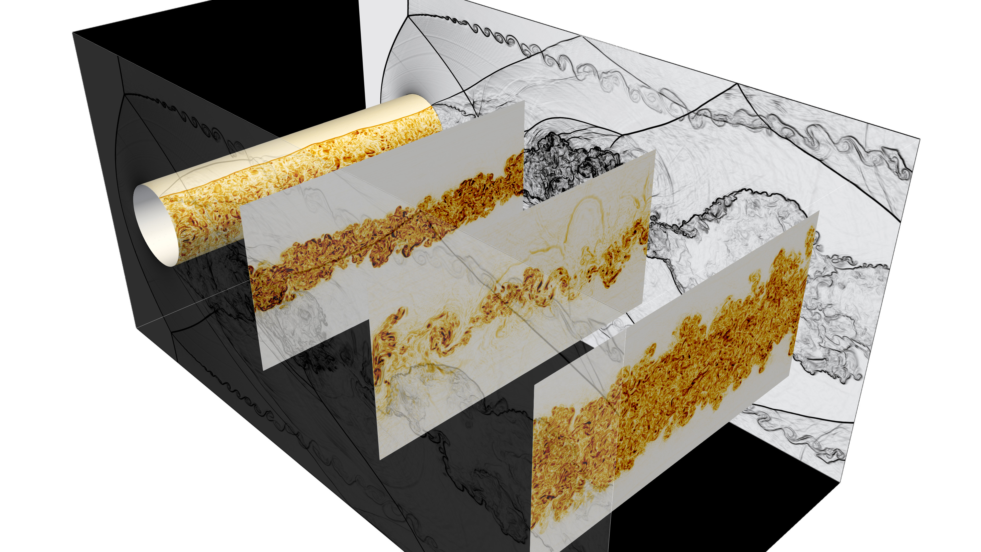
Figure 6. Temporal snapshot of a longer computation of a 3D Mach 3 compressible Euler flow around a disc discretized with 1.8 B Qdofs at $t=5.0$. The two vertical outer cutplanes show a Schlieren plot, i. e., the magnitude of the gradient of the density is shown on an exponential scale from white (low) to black (high). All other cutplanes show the magnitude of the vorticity on a white (low) - yellow (medium) - red (high) scale. The computation was done with an earlier, not fully optimized version of the solver and ran on 30720 MPI ranks with an average time-step size of 6.0e-05. The code achieved an average throughput of 969 QDofs per second (0.04M gridpoints per second per CPU) with a second-order SSP Runge-Kutta time integrator, in contrast to the third-order variant suggested in this paper (see Sec. 3.6).

All computations are performed for a 3D benchmark configuration (Guermond et al., 2018), similar to the 2D configuration shown in Fig. 1, that consists of a supersonic (air) flow at Mach 3 in a rectangular parallelepiped of size $[0,4]\times[-1,1]\times[-1,1]$ past a cylinder with radius $0.25$ is centered along $(0.6,0,z)$, $z\in[-1,1]$. The computational domain is meshed with an unstructured hexahedral coarse mesh and trilinear $\mathcal{Q}_{1}$ elements consisting of 208 gridpoints, or nodal degrees of freedom (Qdofs). A higher resolution is obtained by subdividing every hexahedron into 8 children an appropriate number of times, using a cylindrical manifold to attach newly generated nodes along the cylinder to the curved surface. Fig 6 shows a temporal snapshot at time $t=5.0$ of a typical computation with 1.8B Qdofs.

The hardware used for the experiments in this section is described in Table 1. Both machines are deployed in the form of compute nodes with dual-socket configurations (two CPUs per compute node) with a high-speed network interconnect (Infiniband/Omnipath). The Intel Cascade Lake system has a machine balance of 14.2 Flop/Byte computed from the peak arithemtic throughput and the STREAM triad bandwidth compared to 17.2 Flop/Byte on the Intel Skylake system.

Table 1. Hardware used for the computational experiments and benchmarks. The STREAM triad bandwidth is measured with streaming stores, i.e., it reports the actually transferred data between the cores and the memory.

	Intel Cascade Lake	Intel Skylake
Model name	Xeon Gold 6230	Xeon Platinum 8174
Cores / compute node	$2\times 20$	$2\times 24$
SIMD width	512 bit (AVX-512)	512 bit (AVX-512)
Turbo mode	enabled	disabled
Clock frequency scalar	2.8 GHz	2.3 GHz
Clock frequency AVX-512	2.0 GHz	2.3 GHz
L2 + L3 cache / core	1 MiB + 1.375 MiB	1 MiB + 1.375 MiB
Arithmetic peak with AVX-512 / compute node	2,560 GFlop/s	3,532 GFlop/s
Peak memory bandwidth / compute node	282 GB/s	256 GB/s
STREAM triad bandwidth from RAM / compute node	180 GB/s	205 GB/s

5.1. Roofline performance prediction and kernel selection

The mathematical description of Alg. 1 allows some freedom in rearranging computations between individual loops. In order to find the algorithm variant with the best performance, we need to identify the limiting computational resource. A stencil code such as the one presented in Alg. 1 of sufficient local size, i. e., with more than a few thousand Qdofs per MPI rank, is operated in the throughput regime with respect to communication between the compute nodes. The two primary bottlenecks are thus data access, which is governed by the bandwidth from main memory or caches, and the in-core execution, which can be represented by the roofline performance model (Williams et al., 2009).

5.1.1. Data access

In Table 2 we list the expected memory access of the stages in the final optimized version of the algorithm. All numbers are given as reads and writes per per non-zero entry in the stencil (nnz). The predicted access is reported separately for read transfer (labeled ‘r’ in the table), writes (labeled ‘w’ in the table), and the read-for-ownership transfer (Hager and Wellein, 2011), labeled ‘rfo’ in the table. The read-for-ownership transfer adds additional read transfer for data that is only written. We use non-temporal (streaming) stores for the matrices $d_{ij}$ of step 1, $P_{ij}$ in step 4 and $l_{ij}$ in steps 4 and 5 to avoid the read-for-ownership transfer, but regular stores for the vector data ${\boldsymbol{U}}^{n+1}$ and ${\boldsymbol{R}}^{n+1}$. The performance prediction is based on the following assumptions:

• all big data structures need to be fetched from RAM memory in their entirety for every evaluation step; this includes the matrices $m_{ij},\beta_{ij},\mathbf{c}_{ij}$ and the underlying sparsity pattern as well as the global vectors ${\boldsymbol{U}}^{n}$, ${\boldsymbol{R}}^{n}$, ${\boldsymbol{U}}^{n+1}$, and the vector for the lumped mass matrix;

• access to column data of ${\boldsymbol{U}}^{n}_{j}$ and ${\boldsymbol{R}}^{n}_{j}$, the inverse mass matrix and $\alpha_{j}$ exhibits perfect caching;

• access to the transposed matrix entries $d_{ji}$ and $l_{ji}$ in steps 2, 5 and 6, respectively, exhibits perfect caching with perfect spatial locality.

The last two assumptions regarding data locality of column access are similar to the layer conditions found in high-performance implementations of finite difference stencils (Hager and Wellein, 2011). For example, for the 2D five-point stencil the layer criterion relates the spatial distance of an entry $(i,j)$ to the grid neighbors $(i+1,j)$, $(i-1,j)$, $(i,j+1)$, $(i,j-1)$ to the cache size. In order to only load one data item per update, e. g., the $(i,j+1)$ entry during a lexicographic grid traversal, the cache must be large enough to store two full rows of entries ($2n_{x}$ items, where $n_{x}$ is the number of gridpoints in $x$-direction). For larger mesh sizes the loop must be tiled. The main difference to the present (finite-element) algorithms is the fact that they are written for unstructured meshes with indirect addressing of column data. Thus, a corresponding 3D layer condition for a structured grid requiring that $2n_{x}n_{y}$ items fit into cache has to be modified. A simple imitation of lexicographic numbering for unstructured meshes is obtained by a Cuthill-McKee ordering of the unknowns (Cuthill and McKee, 1969). We can assume that the Cuthill-McKee reordering maintains a bandwidth of approximately $n^{2/3}_{\text{local}}$ unknowns per row, where $n_{\text{local}}$ is the number of DoFs per MPI rank. A modified line criterion could thus be the requirement to hold $2\,n_{\text{local}}^{2/3}$ entries in cache. This implies for the example presented in Table 2 with an average local size of $n_{\text{local}}=358,208$ dofs that about 10,200 entries have to be kept in cache. A state vector ${\boldsymbol{U}}^{n}$ holds five variables per entry. With 8 bytes per double this equates to 400 kiB. Given that the architecture in use provides around 2.4 MiB of L2 and L3 cache combined, we can expect that the modified line criterion is mostly fulfilled in step 1 of the algorithm. On the other hand, in step 4, both vectors ${\boldsymbol{U}}^{n}$ and ${\boldsymbol{R}}^{n}$ amounting to 800 kiB according to the modified layer criterion are required to be maintained in cache, in addition to streaming through the matrices $d_{ij}^{L,n}$ and $m_{ij}$ at the same time. Realistically, step 4 will involve some additional transfer from main memory due to cache eviction.

Table 2. Expected memory transfer and measured performance on a simulation with 29m nodes over 434 time steps (1302 RK stage evaluations), run on 80 Intel Cascade Lake cores (2 compute nodes). Memory bandwidth for STREAM triad is 360 GB/s.

		measurement with likwid			prediction
	time	bandw	read / write	r / w barrier	read / write
	[s]	[GB/s]	[double / nnz]	[double / nnz]	[double / nnz]
step 0: entropies	9.65	239	0.22r + 0.07w	0.29r + 0.09w	0.19r + 0.07w + 0.07rfo
step 1: offdiagonal $d^{L}_{ij}$, $\alpha_{i}$	391.4	132	5.83r + 0.74w	5.46r + 0.65w	4.72r + 0.56w + 0.04rfo
step 2: diagonal $d^{L}_{ii}$, $\tau_{n}$	62.0	304	1.95r + 0.46w	2.44r + 0.56w	1.74r + 0.48w
step 3: low-order update	277.0	222	7.24r + 0.53w	7.21r + 0.51w	5.87r + 0.48w + 0.48rfo
step 4: $P_{ij}$, $l_{ij}$	317.8	248	4.43r + 6.03w	4.31r + 6.04w	3.24r + 6.00w
step 5: h.-o. update, next $l_{ij}$	268.7	260	8.06r + 1.20w	8.21r + 1.21w	6.80r + 1.19w
step 6: final high-order update	132.5	394	6.71r + 0.21w	7.98r + 0.21w	6.69r + 0.19w

Table 2 includes measurements of the memory read and write access to the RAM memory, measured from hardware performance counters recorded with the LIKWID tool (Treibig et al., 2010), version 5.0.1, using an MPI-only experiment. The numbers reported in the table are calculated from the absolute transfer measured with LIKWID, divided by the number of time steps and stages per time step and by the number of nonzero entries in the sparse matrix. The result is further divided by 8, the number of bytes per double, to make the numbers easily comparable to the transfer in terms of Alg. 1. The table includes two sets of measurements of markers around the algorithmic part. The first part measures the sections as they appear in the code. However, the numbers are inaccurate given a load imbalance of 5–15% because the memory transfer is only recorded while the first core of a 20-core CPU resides in the relevant section. If some of the other 19 cores take more time to complete the section (given the implicit barrier via the MPI point-to-point communication at a later stage), the memory transfer appears too low. This effect can be seen by the reads recorded for step 6 of the algorithm, which should be close to step 5 in terms of the transfer, but the reported number is 1.35 doubles less than the theoretical number. In order to obtain more accurate data, we performed a second experiment, labeled “barrier” in Table 2, where MPI barriers are placed around the LIKWID_MARKER_{START/STOP} markers to ensure that only the transfer of the respective section is measured. The write transfer, which is of streaming character, is predicted very well. However, the actual read transfer is by 15%, 40%, 14%, 33%, 21%, and 19% higher than the best-case prediction for steps 1–6, respectively. For steps 1 and 3, the excess transfer is contained because only a single vector ${\boldsymbol{U}}^{n}$ and the entropies, a total of 6 doubles per step, is accessed indirectly and one can expect caches to mostly fit this access, with some minor deviations due to the somewhat unstructured access in the Cuthill–McKee numbering and missing spatial locality. For step 4, the access to both ${\boldsymbol{U}}^{n}$ and ${\boldsymbol{R}}^{n}$ leads to a larger deviation. In steps 2, 5, 6, the excess transfer is due to the transpose access into a sparse matrix, where both the limited size of the caches as well as the transfer of full cache lines rather than single doubles are relevant.

5.1.2. In-core execution

The measured memory throughput in Table 2 demonstrates that only step 6 is at the limit of the memory bandwidth of the architecture, whereas all other steps are primarily limited by the execution inside the core. In order to assess the arithmetic work done by the various stages, Table 3 reports the main characteristics of the floating point performance of the same computation. As discussed in Section 4.6, the nonlinear update steps are heavy on pow(), division and square root operations. Therefore, the arithmetic peak performance of 4 Cascade Lake CPUs with 80 cores in total, 5,120 GFlop/s, is not attainable.

Table 3. Main arithmetic components and measured performance on a simulation with 29m nodes over 434 time steps (1302 RK stage evaluations), run on 80 Intel Cascade Lake cores (2 compute nodes). Arithmetic peak is 5,120 GFlop/s.

	time	measurement with likwid				prediction
	[s]	[GFlop/s]	[Flop/nnz]	[Flop/B]	IPC	[pow()/nnz]	[div/nnz]
step 0: entropies	9.65	848	8	2.6	1.32	0.07	0.04
step 1: offdiagonal $d^{L}_{ij}$, $\alpha_{i}$	391.4	681	262	5.5	0.95	1.08	8.88
step 2: diagonal $d^{L}_{ii}$, $\tau_{n}$	62.0	17	1	0.04	1.65	0	0.04
step 3: low-order update	277.0	892	248	4.0	1.28	1	3.15
step 4: $P_{ij}$, $l_{ij}$	317.8	571	183	2.2	1.16	1–2 (Newton)	2–8
step 5: h.-o. update, next $l_{ij}$	268.7	568	155	2.0	0.97	1–2 (Newton)	2–8
step 6: final high-order update	132.5	91	12	0.18	0.17	0	0

Exemplarily, for step 0 of the algorithm, inspection of the assembly code for the AVX-512 target shows that a single loop iteration consists of 334 instructions. According to the LLVM machine code analyzer (LLVM-MCA), these are predicted to run with a reciprocal throughput of 248 cycles or an instruction-per-cycle (IPC) rate of 1.35. According to the analysis, the main bottleneck is the latency of operations inside the computation of the power function due to data dependencies. More precisely, the polynomial evaluation and division operations in the Padé approximation used in the vectorized pow() implementation (Fog, 2020), as well as the extraction of exponents, have long dependency chains. Since the number of available physical registers and scheduler windows have limited size to keep around 100-200 instructions in flight, little overlap of work from one outer loop iteration (indexed with $i$) with the next one is possible. Among the 334 instructions, there are 69 fused multiply-add operations, 22 additions/substractions, 31 multiplications, and 3 divisions. Given the LLVM-MCA prediction of execution in 248 cycles, this corresponds to a throughput of 0.78 arithmetic operations per cycle, or a utilizatoin of 19.6% of the arithmetic peak performance. The measured performance of 848 GFlop/s corresponds to 17% of the arithmetic peak performance or 85% of the predicted arithmetic throughput. This number matches with the ratio of the measured IPC of 1.32 compared to the predicted IPC of 1.35, showing that the arithmetic operations have been counted correctly. According to the roofline model, the memory bandwidth is not a limiting factor for step 0.

Using similar arguments, it can be shown that steps 1, 3, 4, and 5 of Alg. 1 are limited by the in-core execution on the Cascade Lake processor. Steps 1, 4, and 5 are more strongly effected by long dependency chains that cannot be overlapped sufficiently with independent work. This is evidenced by an IPC prediction of 1.27 for the vectorized pow() function obtained from LLVM-MCA. Step 3 shows a higher performance that is due to a better instruction-level parallelism obtained for the evaluation of ${\mathbbm{f}}({\boldsymbol{U}}^{n}_{j})$ and multiplication with ${\boldsymbol{c}}_{ij}$. Step 2 appears odd (see Table 3) due to a high IPC number but neither high GFlop/s or memory performance. This is because this function is not vectorized. The alternative of computing all of $d_{ij}$ in vectorized form via step 1 instead of the symmetrization would be slower due to the heavy computations in the power function.

Table 4. Measured run times on a simulation with 29m nodes over 434 time steps (1302 RK stage evaluations), run on 96 Intel Skylake cores (2 compute nodes) at 2.3 GHz with hyperthreading off and on, respectively. Memory bandwidth for STREAM triad is 410 GB/s, arithmetic peak 7,066 GFlop/s.

	hyperthreading off			hyperthreading on
	time	arithmetic	bandwidth	time	arithmetic	bandwidth
	[s]	[GFlop/s]	[GB/s]	[s]	[GFlop/s]	[GB/s]
step 0: entropies	7.49	1,094	308	5.68	1,440	404
step 1: offdiagonal $d^{L}_{ij}$, $\alpha_{i}$	295.4	902	177	210.3	1,268	257
step 2: diagonal $d^{L}_{ii}$, $\tau_{n}$	54.2	19	352	50.8	21	381
step 3: low-order update	211.9	1,168	290	212.2	1,166	307
step 4: $P_{ij}$, $l_{ij}$	250.0	726	318	243.4	746	338
step 5: h.-o. update, next $l_{ij}$	225.0	678	317	189.9	803	381
step 6: final high-order update	131.3	92	398	135.3	89	401

5.1.3. Hyperthreading

In order to further assess the performance bottleneck due to latencies in the pipelined execution, we run an additional experiment on 96 Intel Skylake cores comparing enabled and disabled hypertheading; see Table 4. If we run the code with 2-way hyperthreading, scheduling 96 MPI jobs on each compute node, or 192 jobs in total, performance is increased for the latency-limited steps of the algorithm. For example, the run time of step 1 decreases from 295 seconds to 210 seconds, with the arithmetic throughput reaching 18% of the arithmetic peak. Similarly, steps 4 and 5 run considerably faster. On the other hand, step 6 that was already limited by the memory bandwidth with hyperthreading disabled, is slightly slower due to additional memory transfer and increased cache pressure (mainly due to access to transposed entries $l_{ji}$) of the additional thread running on the same core. The performance with hyperthreading on the algorithmic step 3 and, to a lesser extent step 4, is reduced. These steps are affected by additional data streams due to indirect addressing into the column entries of ${\boldsymbol{U}}^{n}_{j}$ and ${\boldsymbol{R}}^{n}_{j}$, which puts a higher strain on address translation and prefetching.

When comparing the absolute run time of the whole solver (without output) for 434 time steps of a three-stage Runge–Kutta integrator, we record 1,292 seconds for Skylake without hyperthreading, 1,164 seconds with hyperthreading, and 1,608 seconds on the slower Intel Cascade Lake system without hyperthreading. The higher performance of the Intel Skylake system is in agreement with the hardware specification; cf. Table 1. As is expected for an architecture with a higher machine balance, many of the components run closer to the memory bandwidth limit. With hyperthreading enabled, step 0, 2, 5 and 6 are now almost entirely limited by the available memory bandwidth. This shows that the optimizations presented in this work have paid off.

5.2. Exploration of algorithmic alternatives

In order to justify the chosen algorithmic layout, we explore a few alternative choices and analyze their performance compared to the results presented in Section 5.1.

5.2.1. Merge step 2 with step 1

In Alg. 1 the symmetry of $d_{ij}^{L}$ was exploited by only computing the upper triangular and diagonal portion of $d_{ij}^{L}$ in step 1 and fixing up the lower triangular part (along with computing the maximal time-step size) in a separate pass (step 2). The memory access in step 2 is non-contiguous and therefore adds additional memory transfer beyond the best-case prediction, as can be seen from Table 2. Given that there is no explicit barrier to fill up the information, apart from the availability of the upper triangular part, this step can be done within the loop of step 1. This promises higher performance because step 1 is limited by the arithmetic operations as described above, so the additional memory transfer can be expected to be partly hidden. As the data in Table 5 shows, the combined time for steps 1 & 2 is larger than with doing the transposition as part of the loop. Despite adding mostly memory access in a core-bound algorithm, there is a small slowdown compared to step 1 executed alone. This is because the lower diagonal part $d_{ij}^{L}$ with $i>j$ for vectorized rows can only be filled up once the complete upper diagonal part of the matrix has been computed. Thus, the instruction-level parallelism given an out-of-order execution window of a few hundreds instructions cannot be fully exploited while waiting for data that is not already prefetched by the hardware. Even though this variant provides slightly higher performance, we do not consider it as the primary algorithm because the basic variant proposed here only works for an MPI-only parallelization. For parallelization with threads, the upper diagonal part to read $d_{ji}^{L}$ is not ready for all rows, and additional re-ordering or additional computations would be necessary.

Table 5. Performance comparison of two variants that merge steps 1 and 2 of Alg. 1: (a) baseline computation with Alg. 1 as reported in Tables 2 and 3; (b) read transpose values from $d_{ji}^{L}$ within compute loop; (c) compute full row of $d_{ij}^{L}$ without explointing symmetry. All tests were run for 1302 Runge–Kutta stage evaluations on 29 million grid points with 80 Cascade Lake cores.

	time	arithmetic	bandwidth	memory read / write
	[s]	[GFlop/s]	[GB/s]	[doubles / nnz]
(a) Baseline: compute $d_{ij}^{L}$ as in Alg. 1 exploiting symmetry
step 1: offdiagonal $d^{L}_{ij}$, $\alpha_{i}$	391.4	681	132	5.83r + 0.74w
step 2: diagonal $d^{L}_{ii}$, $\tau_{n}$	62.0	17	304	1.95r + 0.46w
Variant 1: read transpose values from $d_{ji}^{L}$ within compute loop
step 1+2: complete $d_{ij}^{L}$, $\alpha_{i}$, $\tau_{n}$	415.7	644	164	7.57r + 1.09w
Variant 2: compute full row of $d_{ij}^{L}$ without using symmetry
step 1+2: complete $d_{ij}^{L}$, $\alpha_{i}$, $\tau_{n}$	581.6	669	164	5.45r + 1.09w

Table 5 includes a second variant of the merged steps 1 and 2 that computes all the entries in $d_{ij}^{L}$ without considering symmetry. While the data access is lowest in this case with loads that are mostly streaming, the performance is significantly lower due to the increased number of computations.

Note that writing into $d_{ij}^{L}$ can be done with streaming stores for the baseline algorithm as well as variant 2, where the full $d_{ij}^{L}$ matrix is computed, whereas regular stores with 1 double with read-for-ownership transfer is needed for variant 1 to be able to hit parts of the transposed access in cache.

5.2.2. Split computation of $P_{ij}$ into steps 3 and 4

The contribution $(d_{ij}^{H,n}-d_{ij}^{L,n})({\boldsymbol{U}}^{n}_{j}-{\boldsymbol{U}}^{n}_{i})$ to matrix $P_{ij}$ is already available in step 3 of the algorithm, whereas the baseline algorithm recomputes this information in step 4. Given that both step 3 and 4 are limited by the computations in the core, an algorithmic alternative is to store this temporary result in the storage location of $P_{ij}$ in step 3 and re-load it for the computation of step 4. This incurs writes of five doubles in step 3 (which can be done with streaming stores) and reads of up to four doubles in step 4. On the other hand, $d_{ij}^{L,n}$ and ${\boldsymbol{U}}^{n}_{j}$ do not need to be loaded again in step 4. This modification is reported as variant 3 in Table 6 (b). The results clearly show the additional write data transfer in step 3 and the read transfer in step 4, with both steps running more slowly. The computational time of both steps is significantly increased and the steps are now mostly memory transfer limited. The measured throughput of around 300 GB/s is slightly below the STREAM triad limit of the platform.

While this algorithmic variant is not profitable on the chosen hardware, it can be promising for hardware with high bandwidth-memory interfaces, or when indirect addressing (for example, access to ${\boldsymbol{U}}^{n}_{j}$) is more expensive.

Table 6. Performance comparison of different variants for computing $l_{ij}$ and $P_{ij}$: (a) baseline computation with Alg. 1 as reported in Tables 2 and 3; (b) split computation of $P_{ij}$ into steps 3 and 4 in order to to reduce indirect addressing and computations; (c) compute both $l_{ij}$ and $l_{ji}$ rather than symmetrizing over the memory access the computation of $P_{ij}$ into steps 3 and 4 in order to reduce indirect addressing and computations; (d) do not store the matrix $P_{ij}$ and instead compute the entries on the fly from the respective ingredients in steps 5 and 6 of Alg. 1. All tests were run for 1302 Runge–Kutta stage evaluations on 29 million grid points with 80 Cascade Lake cores and report measured data with LIKWID.

	time	arithmetic	bandwidth	memory read / write
	[s]	[GFlop/s]	[GB/s]	[doubles / nnz]
(a) Baseline: compute $l_{ij}$ and $P_{ij}$ as in Alg. 1
step 3: low-order update	277.0	892	222	7.24r + 0.53w
step 4: $P_{ij}$, $l_{ij}$	317.8	571	248	4.43r + 6.03w
step 5: h.-o. update, next $l_{ij}$	268.7	568	260	8.06r + 1.20w
step 6: final high-order update	132.5	91	394	6.71r + 0.21w
(b) Variant 3: split $P_{ij}$ into two parts
step 3: low-order update, first half of $P_{ij}$	325.2	779	312	7.33r + 5.52w
step 4: second half of $P_{ij}$, $l_{ij}$	358.4	468	292	7.75r + 6.00w
(c) Variant 4: compute both $l_{ij}$ and $l_{ji}$
step 4: $P_{ij}$, $\min(l_{ij},l_{ji})$	558.7	567	152	5.78r + 6.18w
step 5: h.-o. update, next $l_{ij}$	259.2	584	204	5.74r + 1.09w
(d) Variant 5: compute $P_{ij}$ on the fly
step 4: $l_{ij}$	272.2	669	144	4.33r + 1.07w
step 5: h.-o. update, next $l_{ij}$	389.1	507	165	7.14r + 1.21w
step 6: final high-order update	210.9	271	239	6.30r + 0.23w

5.2.3. Compute symmetrization of limiter matrix

In steps 5 and 6, the update of $P_{ij}^{n}$ requires the operation $\min(l_{ij},l_{ji})$, with the latter accessing transpose entries in the matrix. In order to reduce the memory transfer, we analyze a variant 4 of our baseline algorithm that adds the computation of $l_{ji}$ within step 4 of the algorithm. Given that the matrix $P_{ij}$ is skew-symmetric in the sense $\lambda m_{i}P_{ij}=-\lambda m_{j}P_{ji}$, only an additional load to ${\boldsymbol{U}}^{n}_{j}$ and $\texttt{bounds}_{j}$ is needed, in addition to the actual computation in limiter.compute. Table 6 (c) shows an implementation of this variant. While the run time of step 5 and the associated memory access are slightly reduced because the transposed entries are not needed, we observe a noticable increase in execution time in step 4 becausethe simultaneous computation of $l_{ij}$ and $l_{ji}$ in step 4 doubles the number of critical computations. As discussed previously, latency effects inside the limiter are the dominant bottleneck, which explains why the additional computations do not increase the arithmetic throughput. Overall, this option is less attractive because the time gained in step 5 is only minor, given that the gain is mostly due to a reduction in stalls when waiting for the indirectly accessed column data $l_{ji}$ to arrive. A similar modification could be considered for computing the next $l_{ij}$ and $l_{ji}$ in anticipation of step 6. This has similar deficiencies as the alternative discussed above, and in addition needs to wait for the update ${\boldsymbol{U}}^{n+1}_{i}$ to be finished for all columns $\mathcal{I}(j)$.

5.2.4. Computation of entries of $P_{ij}$ on the fly

As a final algorithm variant 5, we consider to skip the storage of $P_{ij}$ and instead evaluated it by the formula ${\boldsymbol{P}}_{ij}=\frac{\tau_{n}}{\lambda m_{i}}\Big{(}\big{(}d_{ij}^{H,n}-d_{ij}^{L,n}\big{)}\big{(}{\boldsymbol{U}}^{n}_{j}-{\boldsymbol{U}}^{n}_{i}\big{)}+b_{ij}{\boldsymbol{R}}_{j}-b_{ji}{\boldsymbol{R}}_{i}\Big{)}$ whenever necessary. This significantly reduces the memory access as the matrix $P_{ij}$ amounts to a read/write of five doubles per non-zero entry, compared to the two matrices $d_{ij}^{L,n}$ and $m_{ij}$ (for computing $b_{ij}$) and the vectors ${\boldsymbol{U}}^{n}_{i}$, ${\boldsymbol{U}}^{n}_{j}$ as well as ${\boldsymbol{R}}_{i}^{n}$, ${\boldsymbol{R}}_{j}^{n}$. Table 6 (d) compares this variant with the baseline algorithm. While step 4 becomes 45 seconds faster by removing the expensive write operation of $P_{ij}$, the additional computations slow down steps 5 and 6 by 120 seconds and 78 seconds, respectively. From the recorded memory transfer, it becomes clear that the gain in transfer is not too high, which can be explained by the fact that besides the two matrices $d_{ij}^{L,n}$ and $m_{ij}$ also indirect addressing to ${\boldsymbol{U}}^{n}_{j}$ and ${\boldsymbol{R}}^{n}_{j}$ needs to be performed. As discussed previously, additional data that is kept in flight increases pressure on the caches and also cache misses, eliminating part of the gain.

5.3. Strong scaling

Since the solver only involves local communication to the neighbors via non-blocking MPI send commands, plus one MPI_Allreduce for computing the time step size, it is straight-forward to run the solver for simulations on large supercomputers. Fig. 7 shows the result of a strong scaling experiment on up to 1,024 compute nodes of Intel Skylake on the SuperMUC-NG machine in Garching, Germany. The experiment is conducted with 2-way hyperthreading enabled using a separate MPI rank for each core and two threads per core. The largest computations are run on 49,152 MPI ranks with 98,304 threads in total. The times reported in this section are based on the minimal time recorded for four runs of the complete time evolution to minimize disturbances from other jobs running on the machine.

Figure 7. Strong and weak scaling of solver on Intel Skylake for problem sizes between 29 million and 15 billion points. The data has been gather by runs using between 434 and 1732 time steps using a three-stage Runge–Kutta scheme and report the run time per time step.

The results in Fig. 7 show an almost perfect scaling to times of around 0.2 seconds per time step or 0.07 seconds per Runge–Kutta stage. The smallest size with 28 million nodes continues to improve throughput all the way to 49k cores with 0.018 seconds per time step. However, the parallel efficiency drops to 46% already for 24k cores, using the run with 1.8 billion unknowns on the same core count as baseline. If we define the strong scaling limit as the point where 80% of the saturated performance is obtained (Fischer et al., 2020), the 29m grid point case scales to 3072 cores (with 81% of parallel efficiency) and the 228m grid point case scales to 12k cores with 89% parallel efficiency. This excellent scalability is the result of judicious algorithmic choices with the majority of communication only between nearest neighbors in the mesh. In each Runge–Kutta stage, one MPI_Allreduce operation is also necessary to control the time step size.

The lowest computational time per Runge–Kutta stage is around $5\times 10^{-3}$ seconds for the proposed algorithm. We can compare this number with the time for one CG iteration of a matrix-free solvers of $2\times 10^{-4}$ seconds on the same SuperMUC-NG system (Arndt et al., 2020, Fig. 8) for the benchmark described in (Fischer et al., 2020) or $10^{-4}$ seconds for the nearest-neighbor communication of a matrix-vector product (Kronbichler and Wall, 2018). The higher limit for scaling in our case can be explained by the significantly more expensive stencil update, as each update involves seven nearest-neighbor communication steps for the various intermediate quantities in the algorithm and one global reduction, which already explains a factor of around ten in the time increase. Furthermore, the computation on 29 million mesh points on 49k cores corresponds to only 290 mesh points per thread, which in itself is a very low value for any PDE-parallel code. Thus, the task granularity is very small at this point, which makes small imbalances in the SIMD/non-SIMD portions more difficult to control. Also, latency effects in the various algorithmic stages, including warm-up of the instruction caching, also play a role at this level. We leave possible improvements along the strong scaling limit to future work (see Remark 4.1).

6. Conclusion and outlook

In this paper we have discussed the efficient implementation of a second-order collocation-type finite-element compressible Euler solver. To this end we started with the mathematical description of the scheme that is guaranteed stable without the need of any tuning parameters. We then reorganized and optimized the given algorithmic structure (Sec. 3) and discussed a scalable high-performance implementation (Sec. 4). The main algorithmic building blocks are traversals through CELL-based sparse matrices with indirect addressing into the solution vector and some auxiliary quantities, as well as a relatively high density of division and transcendental power functions. We demonstrated excellent arithmetic throughput and scaling (Sec. 5) and justified our algorithmic choices against alternatives. We point out a number of possible optimizations that we have not pursued and that we leave for further research and development:

• Further reduction of the number of MPI synchronizations by increasing the overlap of shared cells between neighboring MPI ranks. In our current implementation the overlap is one ghost layer of cells (Arndt et al., 2021). An increased overlap would allow to remove most of the synchronization steps outlined in Fig. 3.

• More efficient coefficient computation of transcendental functions by using a better pipelined custom vectorized pow() implementation as discussed in Sec. 4.6.

• The developed algorithmic structure and the use of a SELL-based sparse matrix format for storage gives hope that the proposed algorithms will also perform reasonably on GPU systems or other HPC architectures. Performance-portable implementations, such as realizations with Kokkos (Edwards et al., 2014) or Raja (Hornung and Keasler, 2014), for this kind of equations are still missing, but could be guided by the performance envelopes and algorithmic behavior identified in the present contribution.

By allowing to modify the mathematical structure we expect an even larger gain in performance of the algorithm:

• The 3D stencil for lowest-order $\mathcal{Q}_{1}$ elements has 27 entries. It is an open research question whether it is possible to reduce the stencil size (for example by additional lumping) for part of the for loops in Alg. 1. In addition, the convex-limiting methodology (Guermond et al., 2018) is not restricted to a CG discretization and can be also applied to (high-order) DG discretizations (Zalesak, 2005; Pazner, 2020). Such flux-corrected DG schemes might promise a higher arithmetic throughput and more regular data access.

• Much of the computational bottleneck stems from the heavy use of the transcendental pow() function. An investigation of modified limiter approaches that still guarantee the invariant-domain property but use a cheaper to evaluate 3-convex function $\Psi({\boldsymbol{U}})$ (Sec. 3.9) thus seems very tempting.

• A similar consideration can be made for the entropy-viscosity commutator (Sec. 3.8) and the subsequent interaction with the limiter: it needs to be investigated whether the number of transcendental functions in the indicator can be reduced by potentially including certain entropies in the limiting process or by using monotonicity/convexity in some functional relations to pull out power functions from the inner $j$ loop to the outer $i$ loop.

- (1)
- Anzt et al. (2020) Hartwig Anzt, Terry Cojean, Chen Yen-Chen, Jack Dongarra, Goran Flegar, Pratik Nayak, Stanimire Tomov, Yuhsiang M. Tsai, and Weichung Wang. 2020. Load-balancing Sparse Matrix Vector Product Kernels on GPUs. ACM Transactions on Parallel Computing 7, 1 (2020), 1–26. https://doi.org/10.1145/3380930
- Arndt et al. (2019) Daniel Arndt, Wolfgang Bangerth, Thomas C. Clevenger, Denis Davydov, Marc Fehling, Daniel Garcia-Sanchez, Graham Harper, Timo Heister, Luca Heltai, Martin Kronbichler, Ross M. Kynch, Matthias Maier, Jean-Paul Pelteret, Bruno Turcksin, and David Wells. 2019. The deal.II Library, Version 9.1. Journal of Numerical Mathematics 27, 4 (2019), 203–213. https://doi.org/10.1515/jnma-2019-0064
- Arndt et al. (2021) Daniel Arndt, Wolfgang Bangerth, Denis Davydov, Timo Heister, Luca Heltai, Martin Kronbichler, Matthias Maier, Jean-Paul Pelteret, Bruno Turcksin, and David Wells. 2021. The deal.II finite element library: design, features, and insights. Computers & Mathematics with Applications 81 (2021), 407–422. https://doi.org/10.1016/j.camwa.2020.02.022
- Arndt et al. (2020) Daniel Arndt, Niklas Fehn, Guido Kanschat, Katharina Kormann, Martin Kronbichler, Peter Munch, Wolfgang A. Wall, and Julius Witte. 2020. ExaDG – High-Order Discontinuous Galerkin for the Exa-Scale. In Software for Exascale Computing – SPPEXA 2016–2019 (Lecture Notes in Computational Science and Engineering 136), Hans-Joachim Bungartz, Severin Reiz, Benjamin Uekermann, Philipp Neumann, and Wolfgang E. Nagel (Eds.). Springer, Cham, 189–224. https://doi.org/10.1007/978-3-030-47956-5_8
- Barlow et al. (2016) Andrew J. Barlow, Pierre-Henri Maire, William J. Rider, Robert N. Rieben, and Mikhail J. Shashkov. 2016. Arbitrary Lagrangian–Eulerian methods for modeling high-speed compressible multimaterial flows. J. Comput. Phys. 322 (2016), 603 – 665. https://doi.org/10.1016/j.jcp.2016.07.001
- Bauer et al. (2018) Simon Bauer, Daniel Drzisga, Marcus Mohr, Ulrich Rüde, Christian Waluga, and Barbara Wohlmuth. 2018. A Stencil Scaling Approach for Accelerating Matrix-Free Finite Element Implementations. SIAM Journal on Scientific Computing 40, 6 (2018), C748–C778. https://doi.org/10.1137/17m1148384
- Bergen et al. (2006) Benjamin Bergen, Tobias Gradl, Frank Hülsemann, and Ulrich Rüde. 2006. A Massively Parallel Multigrid Method for Finite Elements. Computing in Science & Engineering 8, 6 (2006), 56–62. https://doi.org/10.1109/mcse.2006.102
- Brightwell et al. (2005) Ron Brightwell, Rolf Riesen, and Keith D. Underwood. 2005. Analyzing the Impact of Overlap, Offload, and Independent Progress for Message Passing Interface Applications. The International Journal of High Performance Computing Applications 19, 2 (2005), 103–117. https://doi.org/10.1177/1094342005054257
- Cockburn and Shu (1989) Bernardo Cockburn and Chi-Wang Shu. 1989. TVB Runge-Kutta local projection discontinuous Galerkin finite element method for conservation laws. II. General framework. Mathematics of computation 52, 186 (1989), 411–435.
- Cuthill and McKee (1969) Elizabeth Cuthill and James McKee. 1969. Reducing the bandwidth of sparse symmetric matrices. In Proceedings of the 1969 24th national conference of the ACM. ACM Press, New York, 157–172. https://doi.org/10.1145/800195.805928
- Edwards et al. (2014) H. Carter Edwards, Christian R. Trott, and Daniel Sunderland. 2014. Kokkos: Enabling manycore performance portability through polymorphic memory access patterns. J. Parallel and Distrib. Comput. 74, 12 (2014), 3202–3216. https://doi.org/10.1016/j.jpdc.2014.07.003
- Fischer et al. (2020) Paul Fischer, Misun Min, Thilina Rathnayake, Som Dutta, Tzanio Kolev, Veselin Dobrev, Jean-Sylvain Camier, Martin Kronbichler, Tim Warburton, Kasia Świrydowicz, and Jed Brown. 2020. Scalability of high-performance PDE solvers. The International Journal on High Performance Computing Applications in press (2020), 1–25. https://doi.org/10.1177/1094342020915762
- Fog (2020) Agner Fog. 2020. VCL—C++ vector class library manual. Technical Report. https://github.com/vectorclass/version2/releases/download/v2.01.02/vcl_manual.pdf
- Guermond et al. (2018) Jean-Luc Guermond, Murtazo Nazarov, Bojan Popov, and Ignacio Tomas. 2018. Second-order invariant domain preserving approximation of the Euler equations using convex limiting. SIAM J. Sci. Comput. 40, 5 (2018), A3211–A3239. https://doi.org/10.1137/17M1149961
- Guermond et al. (2014) Jean-Luc Guermond, Murtazo Nazarov, Bojan Popov, and Yong Yang. 2014. A second-order maximum principle preserving Lagrange finite element technique for nonlinear scalar conservation equations. SIAM J. Numer. Anal. 52, 4 (2014), 2163–2182. https://doi.org/10.1137/130950240
- Guermond et al. (2011) Jean-Luc Guermond, Richard Pasquetti, and Bojan Popov. 2011. Entropy viscosity method for nonlinear conservation laws. J. Comput. Phys. 230, 11 (2011), 4248–4267. https://doi.org/10.1016/j.jcp.2010.11.043
- Guermond and Popov (2014) Jean-Luc Guermond and Bojan Popov. 2014. Viscous regularization of the Euler equations and entropy principles. SIAM J. Appl. Math. 74, 2 (2014), 284–305. https://doi.org/10.1137/120903312
- Guermond and Popov (2016a) Jean-Luc Guermond and Bojan Popov. 2016a. Fast estimation from above of the maximum wave speed in the Riemann problem for the Euler equations. J. Comput. Phys. 321 (2016), 908–926. https://doi.org/10.1016/j.jcp.2016.05.054
- Guermond and Popov (2016b) Jean-Luc Guermond and Bojan Popov. 2016b. Invariant domains and first-order continuous finite element approximation for hyperbolic systems. SIAM J. Numer. Anal. 54, 4 (2016), 2466–2489. https://doi.org/10.1137/16M1074291
- Guermond and Popov (2017) Jean-Luc Guermond and Bojan Popov. 2017. Invariant Domains and Second-Order Continuous Finite Element Approximation for Scalar Conservation Equations. SIAM J. Numer. Anal. 55, 6 (2017), 3120–3146. https://doi.org/10.1137/16M1106560
- Hager and Wellein (2011) Georg Hager and Gerhard Wellein. 2011. Introduction to High Performance Computing for Scientists and Engineers. CRC Press, Boca Raton.
- Harten (1983) Amiram Harten. 1983. On the symmetric form of systems of conservation laws with entropy. J. Comput. Phys. 49, 1 (1983), 151–164. https://doi.org/10.1016/0021-9991(83)90118-3
- Hoberock (2019) Jared Hoberock. 2019. Working Draft, C ++ Extensions for Parallelism Version 2. Technical Report.
- Hornung and Keasler (2014) Richard D. Hornung and Jeffrey A. Keasler. 2014. The RAJA portability layer: Overview and status. Technical Report 1169830. Lawrence Livermore National Laboratory, Livermore, CA, USA. https://doi.org/10.2172/1169830
- Kreutzer et al. (2014) Moritz Kreutzer, Georg Hager, Gerhard Wellein, Holger Fehske, and Alan R. Bishop. 2014. A Unified Sparse Matrix Data Format for Efficient General Sparse Matrix-Vector Multiplication on Modern Processors with Wide SIMD Units. SIAM Journal on Scientific Computing 36, 5 (2014), C401–C423. https://doi.org/10.1137/130930352
- Kronbichler and Kormann (2012) Martin Kronbichler and Katharina Kormann. 2012. A generic interface for parallel cell-based finite element operator application. Comput. Fluids 63 (2012), 135–147. https://doi.org/10.1016/j.compfluid.2012.04.012
- Kronbichler and Kormann (2019) Martin Kronbichler and Katharina Kormann. 2019. Fast matrix-free evaluation of discontinuous Galerkin finite element operators. ACM Trans. Math. Software 45, 3 (2019), 29:1–29:40. https://doi.org/10.1145/3325864
- Kronbichler and Wall (2018) Martin Kronbichler and Wolfgang A. Wall. 2018. A performance comparison of continuous and discontinuous Galerkin methods with fast multigrid solvers. SIAM Journal on Scientific Computing 40, 5 (2018), A3423–A3448. https://doi.org/10.1137/16M110455X
- Kuzmin and Möller (2005) Dmitri Kuzmin and Matthias Möller. 2005. Algebraic Flux Correction II. Compressible Euler Equations. 207–250. https://doi.org/10.1007/3-540-27206-2_7
- Malas et al. (2018) Tareq M. Malas, Georg Hager, Hatem Ltaief, and David E. Keyes. 2018. Multidimensional Intratile Parallelization for Memory-Starved Stencil Computations. ACM Transactions on Parallel Computing 4, 3 (2018), 12:1–12:32. https://doi.org/10.1145/3155290
- Malas et al. (2015) Tareq M. Malas, Georg Hager, Hatem Ltaief, Holger Stengel, Gerhard Wellein, and David E. Keyes. 2015. Multicore-Optimized Wavefront Diamond Blocking for Optimizing Stencil Updates. SIAM Journal on Scientific Computing 37, 4 (2015), C439–C464. https://doi.org/10.1137/140991133
- OpenMP Architecture Review Board (2015) OpenMP Architecture Review Board. 2015. OpenMP Application Program Interface Version 4.5. Technical Report. https://www.openmp.org/wp-content/uploads/openmp-4.5.pdf
- Pazner (2020) Will Pazner. 2020. Sparse invariant domain preserving discontinuous Galerkin methods with subcell convex limiting. (2020). https://arxiv.org/abs/2004.08503
- Schäfer et al. (1996) Michael Schäfer, Stefan Turek, Franz Durst, Egon Krause, and Rolf Rannacher. 1996. Benchmark computations of laminar flow around a cylinder. In Flow simulation with high-performance computers II. 547–566.
- Shu and Osher (1988) Chi-Wang Shu and Stanley Osher. 1988. Efficient implementation of essentially non-oscillatory shock-capturing schemes. J. Comput. Phys. 77, 2 (1988), 439 – 471. https://doi.org/10.1016/0021-9991(88)90177-5
- Sun et al. (2020) Tianjiao Sun, Lawrence Mitchell, Kaushik Kulkarni, Andreas Klöckner, David A. Ham, and Paul H. J. Kelly. 2020. A study of vectorization for matrix-free finite element methods. The International Journal of High Performance Computing Applications 34, 6 (2020), 629–644. https://doi.org/10.1177/1094342020945005
- Treibig et al. (2010) Jan Treibig, Georg Hager, and Gerhard Wellein. 2010. LIKWID: A lightweight performance-oriented tool suite for x86 multicore environments. In Proceedings of PSTI2010, the First International Workshop on Parallel Software Tools and Tool Infrastructures. IEEE, San Diego CA, 207–216. https://doi.org/10.1109/ICPPW.2010.38
- Wang et al. (2013) Zhijian J. Wang, Krzysztof Fidkowski, Rémi Abgrall, Francesco Bassi, Doru Caraeni, Andrew Cary, Herman Deconinck, Ralf Hartmann, Koen Hillewaert, Hung T. Huynh, Norbert Kroll, Georg May, Per-Olof Persson, Bram van Leer, and Miguel Visbal. 2013. High-order CFD methods: current status and perspective. International Journal for Numerical Methods in Fluids 72, 8 (2013), 811–845. https://doi.org/10.1002/fld.3767
- Wellein et al. (2009) Gerhard Wellein, Georg Hager, Thomas Zeiser, Markus Wittmann, and Holger Fehske. 2009. Efficient Temporal Blocking for Stencil Computations by Multicore-Aware Wavefront Parallelization. In 2009 33rd Annual IEEE International Computer Software and Applications Conference. IEEE, Seattle, WA, USA, 579–586. https://doi.org/10.1109/compsac.2009.82
- Williams et al. (2009) Samuel Williams, Andrew Waterman, and David Patterson. 2009. Roofline: An Insightful Visual Performance Model for Multicore Architectures. Commun. ACM 52, 4 (2009), 65–76. https://doi.org/10.1145/1498765.1498785
- Witherden et al. (2014) Freddie D. Witherden, Antony M. Farrington, and Peter E. Vincent. 2014. PyFR: An open source framework for solving advection–diffusion type problems on streaming architectures using the flux reconstruction approach. Computer Physics Communications 185, 11 (2014), 3028 – 3040. https://doi.org/10.1016/j.cpc.2014.07.011
- Zalesak (2005) Steven T. Zalesak. 2005. The Design of Flux-Corrected Transport (FCT) Algorithms For Structured Grids. 29–78. https://doi.org/10.1007/3-540-27206-2_2