Dynamical Mass Generation in Wick Cutkosky Model

Abstract

Studying extent of dynamical generation of mass in a quantum field theory, which may have non-perturbative attributes, is an essential step towards complete understanding of the theory. The phenomenon has historic relevance to interactions including fermions. However, as searches for further fundamental scalars continue, inquiring into the possibility of dynamical generation of mass becomes crucial for scalars with masses much lower than the electroweak scale. This paper addresses Yukawa interaction between a complex doublet field, named the Higgs for convenience, and a scalar singlet field studied in terms of correlation functions and the dynamical masses produced in the parameter space of the model. An unorthodox approach is adopted to extract the correlation functions and dynamical masses in the model. The study is conducted using the method of Dyson Schwinger equations for the Yukawa coupling $10^{-6}\leq\lambda\leq 2.0$ in GeVs and cutoff $10\leq\Lambda\leq 100$ in TeVs. The scalar masses are found to be around afew MeVs while the Higgs masses are found to be smaller than 1 MeV. The Higgs propagators are found much more sensitive on the coupling than the scalar propagators. The vertices are relatively more stable against the cutoff used in comparison to the propagators and dynamical masses. The model is found to be stable for the cutoff above $100$ TeV. The critical coupling exists in the model and is expected to be in the vicinity of $\lambda=10^{-6}$ GeV. No indications of triviality is found in the model.

1 Introduction

Importance of the standard model (SM) [1, 2] as the theory of low energy phenomenology for particle interactions can not be overstated after the discovery of Higgs boson [3, 4, 5] at the LHC [6, 7, 8]. The discovery also opens a possibility of existence of other fundamental scalars (or pseudo-scalars) in nature, particularly the ones to describe the beyond SM physics, such as Supersymmetry [9, 10, 11, 12, 13], cosmic inflation [14, 15, 16, 17, 18, 19, 20, 21], and dark matter [22, 23, 24, 25, 26] physics. As there exists a wide range of masses in nature from a few orders less than $1$ eV to close to $200$ GeVs, the possibilities of masses for further scalars is a an open question.

One of the main reasons to expect the Higgs was to render the electroweak gauge bosons and several other fundamental particles massive. However, it is a well known fact that the lightest quarks do not direly require Higgs mechanism as they can also generate masses via QCD interactions . With no information regarding the masses of further scalars, studying extent of dynamical generation of masses (DMG) [28, 29, 30, 31, 32, 33, 34, 35, 36, 37, 38, 39] via scalar interactions in various models naturally becomes an important aspect of the scalar sector.

An element of ambiguity in studies related to new physics is that it is not truly known if the new physics is accessible through the approach of perturbation. Furthermore, DMG is a non-perturbative phenomenon by definition. Hence, non-perturbative methods, such as that of Dyson Schwinger Equations (DSEs) [40, 41, 42, 43, 44], become necessary tool to investigate the underlying physics.

However, as is the case with almost every non-perturbative approach, the method of DSEs have a limitation that there may be more unknown correlation functions than the number of considered DSEs. To cope with, it is not uncommon to use ansatz and truncations [40, 41, 42, 43, 37] which may effect the correlation functions. Thus, beside studying the physics, simpler (than the SM, for instance) models offer an extremely important playground for implementing and studying unconventional numerical approaches. A model containing the Yukawa interaction vertex is a highly interesting avenue to study scalar interactions due to its relevance to particle physics phenomenology.

This paper is a continuation of studies of a variant of Wick Cutkosky model [45, 46, 47, 48, 49, 50], and addresses the phenomenon of DMG due to a Yukawa interaction between the Higgs field, which preserves SU(2) symmetry, and a (real) singlet scalar field using the approach of DSEs [40, 41, 42, 43, 44]. There are several benefits such an study offers. Firstly, the model serves as a useful avenue to study how two mutually interacting fields with different symmetries and under the same renormalization condition dynamically acquire masses for various cutoff values. Secondly, understanding features, such as existence of critical coupling and phase structure, in a model containing Yukawa interaction may provide valuable information in searches for new physics. Furthermore, as mentioned above, a relatively simpler interaction offers a test ground to employ uncustomary approaches which could later be used in richer theories.

The model is studied for (bare) coupling values $10^{-6}\leq\lambda\leq 2.0$ in GeVs and cutoff values at $10$ TeV, $50$ TeV, and $100$ TeV. By the definition of DMG, both fields are massless unless they interact.

A significant amount of studies involving scalar interactions is with inclusion of four point interactions in the realm of renormalizable quantum field theories. It includes both the four point self interactions of the Higgs or scalar fields, or the vertex formed by two scalar and two Higgs fields. However, these three types of interactions can also be formed by the three point Yukawa interaction mentioned above. Thus, in this paper only the simpler Yukawa interaction is considered. Inclusion of further vertices are to be reported somewhere else [51] using a different non-perturbative approach [52, 53].

The $\phi^{4}$ theory [54, 55, 56] is found to be trivial [57, 58, 59, 60, 61]. However, despite being a (complex doublet) scalar field, Higgs interactions with gauge bosons in the Yang-Mills-Higgs theory [62, 63] is not found to render the theory trivial. Hence, it is implicitly assumed here that the model considered is not trivial.

This paper encompasses study of the theory in terms of correlation functions and dynamically generated masses using two DSEs for the two field propagators without the truncations or ansatz mentioned above. The DSEs for the two field propagators are used to extract the correlation functions in a numerically controlled environment. The only hard constraints are renormalization conditions, which are typical of renormalizable quantum field theories, and a restriction on the vertex to restrict violent local fluctuations. The equation for least square error is taken as the third equation for the system of three unknown correlation functions. The details are mentioned in the next section.

2 Technical Details

The Euclidean version of the Lagrangian , along with the counter terms [64], is given by

$$\begin{split}L=&(1+A)\delta^{\mu\nu}\partial_{\mu}h^{\dagger}\partial_{\nu}h+(m_{h}^{2}+B)h^{\dagger}h+(1+\alpha)\frac{1}{2}\delta^{\mu\nu}\partial_{\mu}\phi\partial_{\nu}\phi+\\ &\frac{1}{2}(m_{s}^{2}+\beta)\phi^{2}+\lambda(1+\frac{C}{\lambda})\phi h^{\dagger}h\end{split}$$ (1)

with h as the Higgs fields with SU(2) symmetry and $\phi$ a real scalar singlet field. $A$, $B$, $C$, $\alpha$, and $\beta$ are coefficients of the counter terms, and $\lambda$ is the three point interaction coupling. The DSEs for scalar and the Higgs propagators are, respectively, given by

$$\begin{split}S(p)^{-1}=&(1+\alpha)p^{2}+m_{s}^{2}+\beta+\\ &\lambda(1+\frac{C}{\lambda})\int\frac{d^{4}q}{(2\pi)^{4}}H^{ik}(q)\Gamma^{kl}(q,p-q,-p)H^{li}(q-p)\end{split}$$ (2)

$$\begin{split}H^{ij}(p)^{-1}=&\delta^{ij}((1+A)\ p^{2}+m_{h}^{2}+B)\ +\\ &2\lambda(1+\frac{C}{\lambda})\int\frac{d^{4}q}{(2\pi)^{4}}S(q)\Gamma^{ik}(-p,p-q,q)H^{kj}(q-p)\end{split}$$ (3)

where $\Gamma^{kl}(u,v,w)$ is the three point Yukawa interaction vertex of the Higgs, the Higgs bar, and the scalar singlet fields with momenta $u$, $v$, and $w$, respectively. The Higgs and the Higgs bar fields have indices $k$ and $\l$, respectively. $S(p)$ and $H^{ij}(p)$ are scalar propagator and the Higgs propagator, respectively. Setting $m_{s}=0$ and $m_{h}=0$, and introducing the following definitions of $B$ and $\beta$, respectively,

$$B=2\lambda(1+A)(1+\alpha)\sigma_{h}$$ (4)

$$\beta=2\lambda(1+A)(1+\alpha)\sigma_{s}$$ (5)

the dynamical squared masses of the Higgs and scalar fields, respectively, assume the following definitions .

$$m^{2}_{h,d}=2\lambda(1+A)(1+\alpha)\sigma_{h}$$ (6)

$$m^{2}_{s,d}=2\lambda(1+A)(1+\alpha)\sigma_{s}$$ (7)

The vertex is defined as

$$\Gamma^{ik}_{r}=(1+\frac{C}{\lambda})\Gamma^{ik}=(1+A)(1+\alpha)\tilde{\Gamma}^{ik}$$ (8)

Hence, we have the following equations ,

$$\begin{split}S(p)^{-1}=&(1+\alpha)(\ p^{2}+2\lambda(1+A)\sigma_{s}+\\ &\lambda(1+A)\int\frac{d^{4}q}{(2\pi)^{4}}H^{ik}(q)\tilde{\Gamma^{kl}}(q,p-q,-p)H^{li}(q-p))\ \end{split}$$ (9)

$$\begin{split}H^{ij}(p)^{-1}=&(1+A)(\ \delta^{ij}(\ p^{2}+2\lambda(1+\alpha)\sigma_{h})\ +\\ &2\lambda(1+\alpha)\int\frac{d^{4}q}{(2\pi)^{4}}S(q)\tilde{\Gamma^{ik}}(-p,p-q,q)H^{kj}(q-p))\ \end{split}$$ (10)

The renormalization conditions [43] for the propagators are given below .

$$H^{ij}(p)|_{p^{2}=1}=\frac{\delta^{ij}}{p^{2}}|_{p^{2}=1}$$ (11)

$$S(p)|_{p^{2}=1}=\frac{1}{p^{2}}|_{p^{2}=1}$$ (12)

As mentioned below, the quantities $1+A$ and $1+\alpha$ are calculated directly from the renormalization conditions. If the propagators are dominated by tree level contribution, the quantities $(1+A)$, $(1+\alpha)$, and $(1+\frac{C}{\lambda})$ approach 1. As a result, the vertex becomes tree level dominated, see equation 8. Hence, the definition of the vertex in 8 is justified. It is also the reason that in this study computations for all the parameters start with tree level expression for the Higgs propagators, and $\tilde{\Gamma}^{ik}=\lambda$ in magnitude. Since $\tilde{\Gamma}^{ik}$ changes during a computation, the vertex remains without any strict constraints.

No renormalization condition was explicitly imposed on the vertex . The symmetries in the DSEs are numerically implemented while at the same time only the flavor diagonal Higgs propagators are assumed to be non-vanishing in order to maintain the similarity between the Higgs propagator and its tree level structure.

Interpolation is performed on scalar propagator to implement the renormalization condition 12. Since the two DSEs, 9 and 10 are nonlinearly coupled, $m^{2}_{h,d}\geq 0$ and $m^{2}_{s,d}\geq 0$ are imposed in order to suppress the artifacts due to interpolations.

As there is no DSE or ansatz used for the Yukawa vertex, three steps are taken to ensure that the resulting correlation functions, particularly the vertex, are stable. Firstly, a condition is locally imposed on the vertex that it never exceeds an order of magnitude relative to its neighboring momentum points in the 4-momentum (Euclidean) spacetime. The constraint is similar to the well known Lipschitz condition abundantly used in literature [65, 66, 67, 68, 69]. The constraint is introduced to keep the vertex from fluctuating violently. Secondly, instead of calculating local deviations, sum of squared errors is calculated, which leads to implementation of least squares method with the equation given below.

$$\begin{split}\int dp(\ H^{ij}(p)^{-1}-&(\ (1+A)(\ \delta^{ij}(\ p^{2}+2\lambda(1+\alpha)\sigma_{h})\ +2\lambda(1+\alpha)\\ &\int\frac{d^{4}q}{(2\pi)^{4}}S(q)\tilde{\Gamma^{ik}}(-p,p-q,q)H^{kj}(q-p))\ )\ )\ ^{2}=0\end{split}$$ (13)

It certainly slows the computations but it is found enormously helpful in improving stability of the correlation functions. It also serves as the third equation and, hence, fulfilling the requirement of the third equation for the three correlation functions to be calculated . Furthermore, the solution becomes an optimization problem in which 13 is to be minimized.

Lastly, the Higgs propagators are expanded in the polynomial form given below.

$$H^{ij}(p)=\delta^{ij}\frac{1}{c(p^{2}+d+f(p))}$$ (14)

with $f(p)$ defined as

$$f(p)=\frac{\displaystyle\sum_{i=0}^{N}a_{i}p^{2i}}{\displaystyle\sum_{l=0}^{N}b_{l}p^{2l}}$$ (15)

where $a_{i}$, $b_{l}$, $c$, and $d$ are parameters to be updated during a computation. Such a parameterization brings certain advantages. Firstly, the procedure of renormalization is significantly faster than the alternative approaches which may involve interpolations. Secondly, there is a certain correspondence between the self energy contribution and the expansion in equations 10 and 15, which renders the vertex a certain form. Hence, a stable vertex is achieved whose fluctuations mostly depend upon the resolution among momentum values.

The computation proceeds as follows: It starts with tree level structures for the Higgs propagators and the vertex , and the parameters $\sigma_{s}$ and $\sigma_{h}$ are set to zero. The scalar propagator takes the values from its DSE, see equation 9. First, $\sigma_{s}$ is calculated using Newton Raphson’s method. The criterion for acceptance of update is minimization in equation 13, i.e. the value of the integral in the equation decreases. If an update does not decrease the value, it is not accepted. The same method is used to update the Higgs propagator, the vertex, and $\sigma_{h}$. Update of $\sigma_{s}$ is followed by that of $\sigma_{h}$ parameter.

Next is the update of the parameters in equation 14 for the Higgs propagators. Lastly, the function $\tilde{\Gamma^{ik}}$ is updated at each momentum value while preserving the symmetry imposed by the DSEs. During updating of each of the above mentioned quantities, scalar propagator is calculated from equation 9. The quantities $1+A$ and $1+\alpha$ are calculated during each update and calculation of the Higgs and scalar propagators, respectively.

Hence, as a computation proceeds, $\sigma_{s}$ and $\sigma_{h}$ deviate from their starting value, while the Higgs propagators and the vertex numerically deviate from their tree level structures . The computation ends when either there is no further improvement in the sum of squared errors or it has reached a value below the preset value for the sum of squared errors. The minimum error is preset at $10^{-20}$.

It was found that changing the sequence of updates of the parameters or the correlation functions does not effect the results within machine precision. It was taken as the definition of uniqueness through out the study.

The model is studied with interactions taking place on a plane immersed in the 4 dimensional Euclidean spacetime. Gauss quadrature algorithm is used for numerical integration.

The algorithms are developed in C++ environment and ROOT, CERN is used for constructing the presented diagrams.

3 Correlation Functions

3.1 Field Propagators

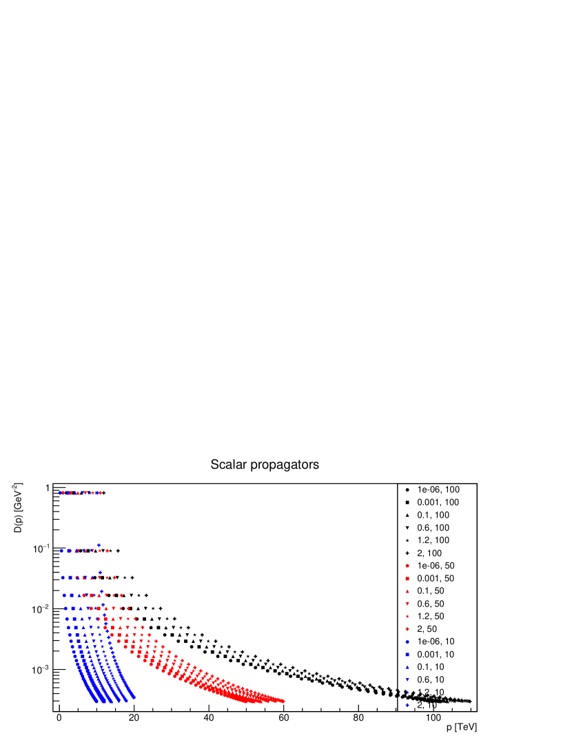
Figure 1: Scalar propagators for different couplings $\lambda$ (in GeVs) and cutoff values $\Lambda$ (in TeVs), shown as ($\lambda$,$\Lambda$) in the legend, are plotted. Starting with the highest value of coupling constant for a fixed cutoff, each subsequent scalar propagator with lower coupling constant is displaced by 2 TeV momentum in the figure.

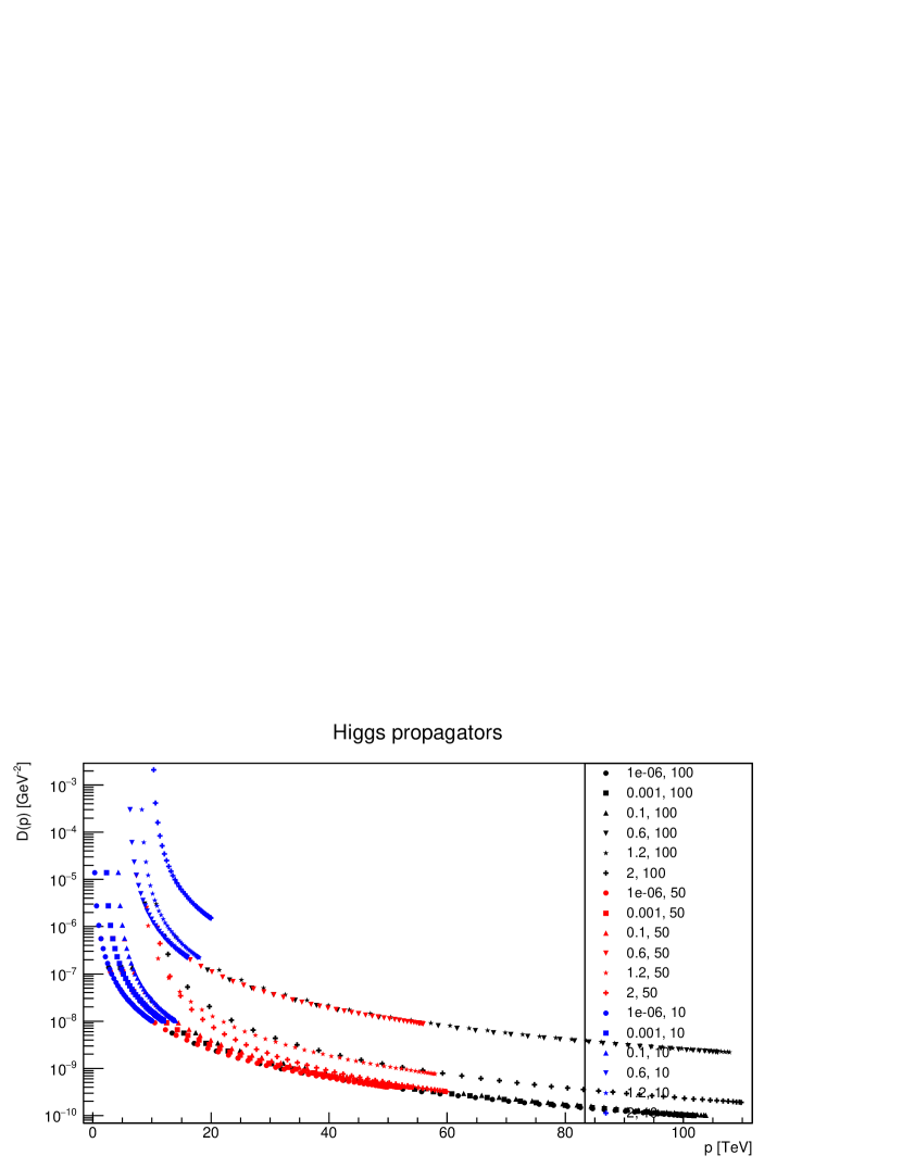
Figure 2: Higgs propagators for different couplings $\lambda$ (in GeVs) and cutoff values $\Lambda$ (in TeVs), shown as ($\lambda$,$\Lambda$) in the legend, are plotted. Starting with the highest value of coupling constant for a fixed cutoff, each subsequent Higgs propagator with lower coupling constant is displaced by 2 TeV momentum in the figure.

The scalar and the Higgs propagators are shown in figures 1 and 2, respectively. For the case of scalar propagators, the most interesting feature is their strong (qualitative as well as quantitative) similarity for various couplings. It points towards the possibility that the model favors a certain narrow range of dynamical scalar masses which, in an extreme case, can even be a particular value characteristic to the model. In fact, it was the Higgs propagator which was expected to be stable due to the reason that Higgs mass was found to be less sensitive [70]. However, the presence of cutoff effects in the propagators is severe enough to expect cutoff dependence of scalar mass. The effects become milder for higher cutoff which is an indication of absence of coupling dependence as the cutoff value reaches the order of hundreds of TeV, see figure 1. Overall, the propagators are found enhanced as the coupling increases for all cutoff values. It is an indication of the role of the quantity $1+\alpha$ in equation 9.

In contrast to the scalar propagators, the Higgs propagators posses different features. First of all, they are sensitive to coupling as well as the cutoff values. For the coupling values considerably lower than 1.0 GeV, Higgs propagators are found to be suppressed. The propagators are enhanced as the coupling rises to the vicinity of 1.0 GeV. However, signs of similar suppression are observed once again for further higher coupling values. This change in behavior is peculiar since it takes place in the vicinity of $\lambda=0.6$ GeV which is close to the fourth root of quartic self interaction coupling for Higgs. Furthermore, as is the case for scalar propagators, there are cutoff effects for higher coupling values.

Both propagators loose dependence on cutoff in TeVs and coupling lower than $10^{-3}$ GeV coupling values. It is the first clue that the masses might have approached a value characteristic to the model.

3.2 Higgs-scalar vertices

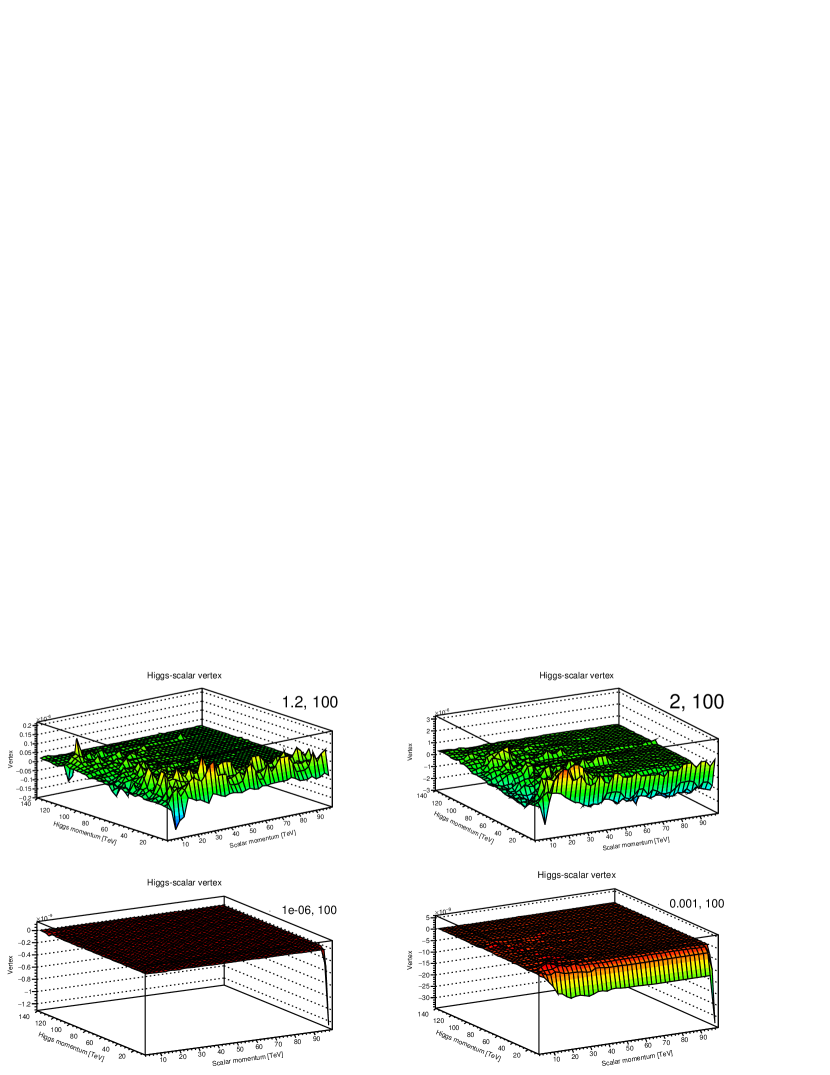
Figure 3: Yukawa interaction vertices between Higgs and scalar fields are shown for various couplings (in GeV) with cutoff at $100$ TeV.

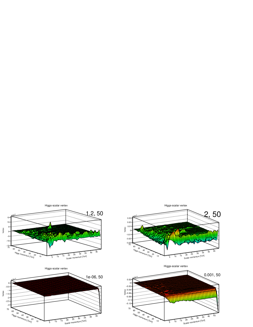
Figure 4: Yukawa interaction vertices between Higgs and scalar fields are shown for various couplings (in GeV) with cutoff at $50$ TeV.

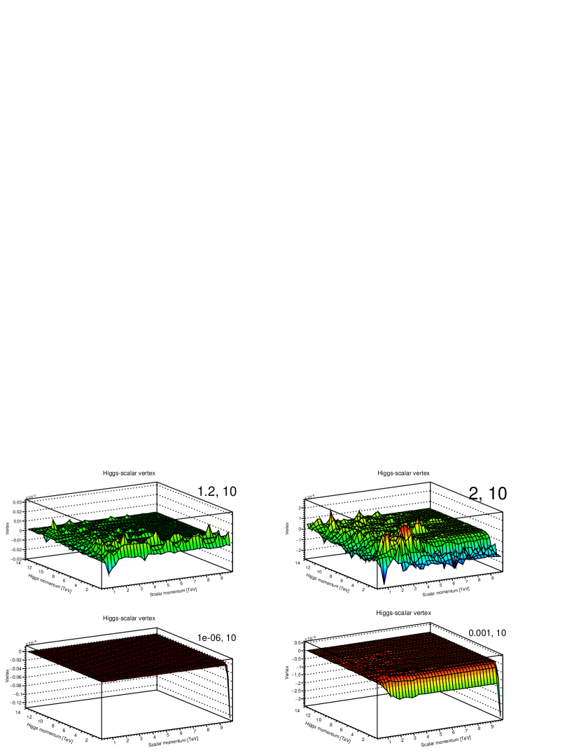
Figure 5: Yukawa interaction vertices between Higgs and scalar fields are shown for various couplings (in GeV) with cutoff at $10$ TeV.

The Yukawa interaction vertices, defined in equation 8, are shown in figures 3, 4, and 5 for various coupling values with cutoff at $100$ TeV, $50$ TeV, and $10$ TeV, respectively .

Firstly, the vertex is found to have qualitative dependence on the field momenta, see figures 3 to 5. A peculiar observation is the similarity of the vertices for $\lambda\leq 10^{-3}$ GeV irrespective of the cutoff. It suggests that the physics (at around or) below this coupling value does not change much.

For higher couplings the vertices do not resume their behavior at low coupling values, which was observed for the Higgs propagators. It is a sign that for higher values of coupling, the dynamical masses may behave differently over coupling. Since such a qualitative dependence is not in harmony with scalar propagators, as they have weak dependence on the coupling, it suggests that the Higgs’ role may be relatively more prominent than that of scalar field in the phenomenon of dynamical mass generation.

The vertex is also found to have weak cutoff dependence at higher couplings. It supports the speculation that it may be the masses whose cutoff effects translate to the propagators, see equations 9 and 10.

Qualitative dependence on field momenta is a clear indication that the theory is not a trivial theory and the deviations in the Higgs propagators are more than a mere multiplicative constant to the corresponding tree level structure due to the contribution by self energy term, see equation 10. It indicates that the extracted correlation functions may differ from the studies with assumtion that the vertex is fixed at a certain value value for all field momenta.

4 Dynamical Renormalized Masses

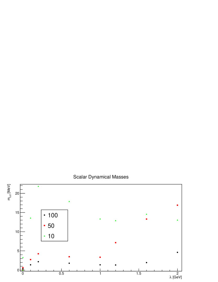
Figure 6: Dynamically generated masses of scalar field $m_{s}$ as a function of Yukawa coupling $\lambda$ at different cutoff values (in TeVs) are shown.

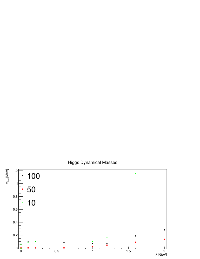
Figure 7: Dynamically generated squared masses of the Higgs field $m_{s}$ as a function of Yukawa coupling $\lambda$ at different cutoff values (in TeVs) are shown.

The dynamical masses are plotted in figures 6 and 7 for scalar and the Higgs fields, respectively. An immediate observation is strong cutoff effects on masses of both fields. For the case of DMG, the renormalized masses do not have any contribution from tree level value. It is also the reason that the cutoff effects appear vividly in the figures 6 and 7 and can not hide behind the bare mass. Indication of stability in the masses ensues only above 100 TeVs.

For the case of scalar mass, it remains within afew MeVs for most of the coupling values at higher cutoff. This observation is not entirely unexpected as the stability of the scalar propagators has already suggested it. However, peculiar to the model is the magnitude of the mass which is in the vicinity of the lightest quarks [3].

The Higgs dynamical mass is found to be less than 0.5 MeV, significantly lower than the scalar mass. It demonstrates how dynamics of the fields with different symmetries differ from each other in a model despite the fact that statistically they are of the same type of fields.

Dynamical masses for both fields remains non-vanishing for $2.0\leq\lambda\leq 10^{-3}$ but are found to be zero at $\lambda=10^{-6}$ GeV. Hence, based upon their dependence on the coupling, it is concluded that the critical coupling may exist in the vicinity of $\lambda=10^{-6}$ GeV.

Despite the difference in magnitudes, the cutoff at which the masses tend to stabilize is over a hundred TeV. In comparison to the QCD physics, this observation can be attributed to the simplicity of the model which does not contain any but a Yukawa interaction.

5 Conclusion

The current study is an addition to exploration of Wick Cutkosky model using the method of DSEs with a different approach. It is found that even a Yukawa interaction can dynamically generate scalar masses of the magnitude close to the already existing fundamental particles.

The propagators as well as the masses can be differentiated for the two fields. Hence, the study also serves as a demonstrator of how two fields of the same nature but different symmetries in the theory menifest themselves. The vertices are least effected by the cutoff.

As is the case with QCD interactions, the model is found to be producing masses in MeVs which serves as another limitation on the extent of dynamical mass generation. However, an important difference is that the masses stabilize over most of the coupling values for cutoff above 100 TeVs. Hence, the model serves as a reminder of the remarkable strength and diversity of QCD interactions which could be competed, though in a restricted sense, with a Yukawa interaction only at relatively much higher cutoff values.

It was found that there is indeed a critical coupling for the model at around $10^{-6}$ GeV.

model is an addition to the observation that the Higgs interaction with other fields does not render the theory trivial. Thus, it begs for further investigation of the scalar sector in the models richer than the one studied here.

6 Acknowledgments

I am deeply indebted to Dr. Shabbar Raza and Dr. Rizwan Khalid for a number of valuable discussions during this endeavor. I would also like to express my deepest gratitude to Professor Johan Hansson for his critical advices and inspiration by some of his work.

This work was supported by Lahore University of Management Sciences, Pakistan.

References

- [1] Matthew D. Schwartz. Quantum Field Theory and the Standard Model. Cambridge University Press, 2014.
- [2] R. Michael Barnett et al. Particle physics summary. Rev. Mod. Phys., 68:611–732, 1996.
- [3] J. Beringer et al. (Particle Data Group). Phys. Rev. D, 86:010001, 2012.
- [4] Axel Maas. Brout-Englert-Higgs physics: From foundations to phenomenology. 2017.
- [5] Marcela Carena and Howard E. Haber. Higgs boson theory and phenomenology. Prog. Part. Nucl. Phys., 50:63–152, 2003.
- [6] Georges Aad et al. Observation of a new particle in the search for the Standard Model Higgs boson with the ATLAS detector at the LHC. Phys. Lett., B716:1–29, 2012.
- [7] Serguei Chatrchyan et al. Observation of a new boson at a mass of 125 GeV with the CMS experiment at the LHC. Phys. Lett., B716:30–61, 2012.
- [8] M. Malbertion. SM Higgs boson measurements at CMS. Nuovo Cim., C40(5):182, 2018.
- [9] Gordon Kane. Exciting Implications of LHC Higgs Boson Data. 2018.
- [10] Howard E. Haber and Yosef Nir. Multiscalar Models With a High-energy Scale. Nucl. Phys., B335:363–394, 1990.
- [11] John F. Gunion and Howard E. Haber. The CP conserving two Higgs doublet model: The Approach to the decoupling limit. Phys. Rev., D67:075019, 2003.
- [12] Stephen P. Martin. A Supersymmetry primer. 1997. [Adv. Ser. Direct. High Energy Phys.18,1(1998)].
- [13] Morad Aaboud et al. Search for electroweak production of supersymmetric states in scenarios with compressed mass spectra at TeV with the ATLAS detector. Submitted to: Phys. Rev. D, 2017.
- [14] Fedor Bezrukov. The Higgs field as an inflaton. Class. Quant. Grav., 30:214001, 2013.
- [15] Andrei D. Linde. Particle physics and inflationary cosmology. Contemp. Concepts Phys., 5:1–362, 1990.
- [16] V. Mukhanov. Physical Foundations of Cosmology. Cambridge University Press, Oxford, 2005.
- [17] Vera-Maria Enckell, Kari Enqvist, Syksy Rasanen, and Eemeli Tomberg. Higgs inflation at the hilltop. 2018.
- [18] Alan H. Guth. The Inflationary Universe: A Possible Solution to the Horizon and Flatness Problems. Phys. Rev., D23:347–356, 1981.
- [19] J. G. Ferreira, C. A. de S. Pires, J. G. Rodrigues, and P. S. Rodrigues da Silva. Inflation scenario driven by a low energy physics inflaton. Phys. Rev., D96(10):103504, 2017.
- [20] Rémi Hakim. The inflationary universe : A primer. Lect. Notes Phys., 212:302–332, 1984.
- [21] Andrei D. Linde. Hybrid inflation. Phys. Rev., D49:748–754, 1994.
- [22] Peter Athron et al. Status of the scalar singlet dark matter model. Eur. Phys. J., C77(8):568, 2017.
- [23] Jae-Weon Lee. Brief History of Ultra-light Scalar Dark Matter Models. EPJ Web Conf., 168:06005, 2018.
- [24] M. C. Bento, O. Bertolami, R. Rosenfeld, and L. Teodoro. Selfinteracting dark matter and invisibly decaying Higgs. Phys. Rev., D62:041302, 2000.
- [25] Orfeu Bertolami, Catarina Cosme, and João G. Rosa. Scalar field dark matter and the Higgs field. Phys. Lett., B759:1–8, 2016.
- [26] Carlos Munoz. Models of Supersymmetry for Dark Matter. 2017. [EPJ Web Conf.136,01002(2017)].
- [27] Johan Hansson. Physical Origin of Elementary Particle Masses. Electron. J. Theor. Phys., 11(30):87–100, 2014.
- [28] Tomas Brauner and Jiri Hosek. Dynamical fermion mass generation by a strong Yukawa interaction. Phys. Rev., D72:045007, 2005.
- [29] Pieter Maris and Peter C. Tandy. Bethe-Salpeter study of vector meson masses and decay constants. Phys. Rev., C60:055214, 1999.
- [30] Christian S. Fischer and Reinhard Alkofer. Nonperturbative propagators, running coupling and dynamical quark mass of Landau gauge QCD. Phys. Rev., D67:094020, 2003.
- [31] A. C. Aguilar, A. V. Nesterenko, and J. Papavassiliou. Infrared enhanced analytic coupling and chiral symmetry breaking in QCD. J. Phys., G31:997, 2005.
- [32] Patrick O. Bowman, Urs M. Heller, Derek B. Leinweber, Maria B. Parappilly, Anthony G. Williams, and Jian-bo Zhang. Unquenched quark propagator in Landau gauge. Phys. Rev., D71:054507, 2005.
- [33] A. C. Aguilar and J. Papavassiliou. Chiral symmetry breaking with lattice propagators. Phys. Rev., D83:014013, 2011.
- [34] Ian C. Cloet and Craig D. Roberts. Explanation and Prediction of Observables using Continuum Strong QCD. Prog. Part. Nucl. Phys., 77:1–69, 2014.
- [35] Mario Mitter, Jan M. Pawlowski, and Nils Strodthoff. Chiral symmetry breaking in continuum QCD. Phys. Rev., D91:054035, 2015.
- [36] Daniele Binosi, Lei Chang, Joannis Papavassiliou, Si-Xue Qin, and Craig D. Roberts. Natural constraints on the gluon-quark vertex. Phys. Rev., D95(3):031501, 2017.
- [37] Alejandro Ayala, Adnan Bashir, Alfredo Raya, and Eduardo Rojas. Dynamical mass generation in strongly coupled quantum electrodynamics with weak magnetic fields. Phys. Rev., D73:105009, 2006.
- [38] M. V. Libanov and V. A. Rubakov. More about spontaneous Lorentz-violation and infrared modification of gravity. JHEP, 08:001, 2005.
- [39] Petr Benes, Tomas Brauner, and Adam Smetana. Dynamical electroweak symmetry breaking due to strong Yukawa interactions. J. Phys., G36:115004, 2009.
- [40] Julian S. Schwinger. On the Green’s functions of quantized fields. 1. Proc. Nat. Acad. Sci., 37:452–455, 1951.
- [41] Julian S. Schwinger. On the Green’s functions of quantized fields. 2. Proc. Nat. Acad. Sci., 37:455–459, 1951.
- [42] Eric S. Swanson. A Primer on Functional Methods and the Schwinger-Dyson Equations. AIP Conf.Proc., 1296:75–121, 2010.
- [43] Craig D. Roberts and Anthony G. Williams. Dyson-Schwinger equations and their application to hadronic physics. Prog. Part. Nucl. Phys., 33:477–575, 1994.
- [44] R. J. Rivers. PATH INTEGRAL METHODS IN QUANTUM FIELD THEORY. Cambridge University Press, 1988.
- [45] Tajdar Mufti. Exploring Higgs boson Yukawa interactions with a scalar singlet using Dyson-Schwinger equations. 2018.
- [46] Jurij W. Darewych. Some exact solutions of reduced scalar Yukawa theory. Can. J. Phys., 76:523–537, 1998.
- [47] Vladimir B. Sauli. Nonperturbative solution of metastable scalar models: Test of renormalization scheme independence. J. Phys., A36:8703–8722, 2003.
- [48] G. V. Efimov. On the ladder Bethe-Salpeter equation. Few Body Syst., 33:199–217, 2003.
- [49] E. Ya. Nugaev and M. N. Smolyakov. Q-balls in the Wick–Cutkosky model. Eur. Phys. J., C77(2):118, 2017.
- [50] J. W. Darewych and A. Duviryak. Confinement interaction in nonlinear generalizations of the Wick-Cutkosky model. J. Phys., A43:485402, 2010.
- [51] Tajdar Mufti. Higgs-scalar singlet system with lattice simulations. unpublished.
- [52] Heinz J. Rothe. Lattice Gauge Theories, An Introduction. World Scientific, London, 1996. London, UK: world Scientific (1996) 381 p.
- [53] Christof Gattringer and Christian B. Lang. Quantum chromodynamics on the lattice. Lect. Notes Phys., 788:1–343, 2010.
- [54] A. Hasenfratz, K. Jansen, J. Jersak, C. B. Lang, T. Neuhaus, and H. Yoneyama. Study of the Four Component phi**4 Model. Nucl. Phys., B317:81–96, 1989.
- [55] F. Gliozzi. A Nontrivial spectrum for the trivial lambda phi**4 theory. Nucl. Phys. Proc. Suppl., 63:634–636, 1998.
- [56] A. Weber, J. C. Lopez Vieyra, Christopher R. Stephens, S. Dilcher, and P. O. Hess. Bound states from Regge trajectories in a scalar model. Int. J. Mod. Phys., A16:4377–4400, 2001.
- [57] Renata Jora. theory is trivial. Rom. J. Phys., 61(3-4):314, 2016.
- [58] Michael Aizenman. Proof of the Triviality of phi d4 Field Theory and Some Mean-Field Features of Ising Models for d¿4. Phys. Rev. Lett., 47:886–886, 1981.
- [59] Peter Weisz and Ulli Wolff. Triviality of theory: small volume expansion and new data. Nucl. Phys., B846:316–337, 2011.
- [60] Johannes Siefert and Ulli Wolff. Triviality of theory in a finite volume scheme adapted to the broken phase. Phys. Lett., B733:11–14, 2014.
- [61] Matthijs Hogervorst and Ulli Wolff. Finite size scaling and triviality of theory on an antiperiodic torus. Nucl. Phys., B855:885–900, 2012.
- [62] Axel Maas and Tajdar Mufti. Two- and three-point functions in Landau gauge Yang-Mills-Higgs theory. JHEP, 04:006, 2014.
- [63] Axel Maas and Tajdar Mufti. Spectroscopic analysis of the phase diagram of Yang-Mills-Higgs theory. Phys. Rev., D91(11):113011, 2015.
- [64] Ashok Das. Lectures on quantum field theory. 2008.
- [65] A. M. Gupal. Minimizing method for functions that satisfy the lipschitz condition. Cybernetics, 16(5):733–737, Sep 1980.
- [66] Feng Gu. Iterative process for certain nonlinear mappings with lipschitz condition. Applied Mathematics and Mechanics, 22(12):1458–1467, Dec 2001.
- [67] Gunnar Aronsson. Extension of functions satisfying lipschitz conditions. Arkiv för Matematik, 6(6):551–561, Jun 1967.
- [68] A. A. Zevin. Extremal periodic solutions of differential equations with generalized lipschitz condition. Doklady Mathematics, 84(2):620–624, Oct 2011.
- [69] J. A. Ezquerro and M. A. Hernández-Verón. On the domain of starting points of newton’s method under center lipschitz conditions. Mediterranean Journal of Mathematics, 13(4):2287–2300, Aug 2016.
- [70] Holger Gies, René Sondenheimer, and Matthias Warschinke. Impact of generalized Yukawa interactions on the lower Higgs mass bound. Eur. Phys. J., C77(11):743, 2017.