Curve shortening flow on Riemann surfaces with possible ambient conic singularities

Abstract.

In this paper, we study the curve shortening flow (CSF) on Riemann surfaces. We generalize Huisken’s comparison function to Riemann surfaces and surfaces with conic singularities. We reprove the Gage-Hamilton-Grayson theorem on surfaces. We also prove that for embedded simple closed curves, CSF can not touch conic singularities with cone angles smaller than or equal to $\pi$.

1. Introduction

In this paper, we study curve shortening flow (CSF) on surfaces. Let $(M,g)$ be a compact Riemann surface. We consider a one-parameter family of simple closed curves $\{\Gamma_{t}\}_{t\in[0,T)}$ on $M$. Suppose that $\Gamma_{t}$ is parametrized by

$$X :S^{1}\times[0,T)\to M.$$

We call $\{\Gamma_{t}\}$ a curve shortening flow on $M$ if

$$\frac{\partial}{\partial t}X(u,t)=k\boldsymbol{n},$$

where $k$ is the geodesic curvature and $\boldsymbol{n}$ the normal vector at $X(u,t)$. We only consider CSF for embedded simple closed curves.

The classic Gage-Hamilton-Grayson Theorem states that: A smooth embedded closed curve will stay smooth and embedded under CSF unless it converges to a single round point. See [GH86, Gra87, Gra89, Gag90]. Here a round point means by a rescaling procedure, the limiting curve is a round circle. Huisken gives an alternative proof for planar curves [Hui98]. His proof utilizes a monotonic comparison function aimed at the isoperimetric profile on $\mathbb{R}^{2}$.

In this paper, we generalize Huisken’s proof to surfaces and give an alternative proof of Gage-Hamilton-Grayson theorem. A key construction is the following function which is inspired by Huiksen’s comparison function [Hui98]:

(1.1) $$R(t)=\sup_{x,y}\frac{L(t)e^{-Kt}}{\pi d(x,y,t)}\sin\left(\frac{\pi l(x,y,t)}{L(t)}\right),$$

where $d(x,y,t)$ is the distance between $X(x,t)$ and $X(y,t)$, $L(t)$ is the total length of $X(\cdot,t)$, and $l(x,y,t)$ is the arc-length between $x$ and $y$. We state our first main result.

Theorem 1.1.

Suppose that $X:S^{1}\times[0,T)\to M$ is a curve shortening flow. Let $R(t)$ be the comparison function defined in (1.1). Let $d_{M}$ be the injectivity radius and $K_{M}=\sup_{M}|\mathcal{K}|$ be the Gaussian curvature bound. Suppose that the curve shortening flow exists in the time period $[0,T)$. There exists a constant $K=K(d_{M},K_{M})$ such that $R(t)$ is bounded by a constant $C(R(0),d_{M},K_{M})$ .

Remark 1.2.

One can not expect $R(t)$ to be monotonic. In fact, we can only perform variation of distance function inside a small neighborhood. So the bound of $R(t)$ can be huge. However, the boundedness of $R(t)$ is enough to rule out Type II singularities. See Section 2. Brendle [Bre14] gives a nice exposition for some generalizations of Huisken’s comparison functions.

Together with an analysis on Type I singularities in Section 5, we can prove Gage-Hamilton-Grayson Theorem:

Theorem 1.3.

Suppose that $\Gamma_{t}$ is a curve shortening flow starting with a smooth embedded curve. Then, $\Gamma_{t}$ remains smooth and embedded unless it converges to a round point.

Remark 1.4.

Our approach follows from Huisken’s proof [Hui98] on planar curves which is summarized in Section 2. Andrews and Bryan [AB11] also give a proof for planar CSF by constructing a very delicate comparison function.

It is worth noting that our comparison function can be applied to CSF on conic Riemann surfaces. Conic Riemann surfaces are surfaces with cone-like singularities. The simplest example is the flat cone

(1.2) $$C_{a\pi}=(\mathbb{C},g_{a\pi}),g_{a\pi}=|z|^{a-2}|dz|^{2},$$

for some $0<a$. It has a conic singularity at the origin with cone angle $a\pi$ if $0<a\pi<2\pi$.

Now, imagine curve shortening flow on $C_{\alpha\pi}$ as a shrinking rubber band. See Figure 1.1.

Figure 1.1. CSF on flat cones

There are two cases: If the cone angle is big, the cone tip is not a big obstacle and the rubber band can move across the cone tip to another side. In the extreme case $\alpha=2$, $C_{2\pi}$ is just $\mathbb{R}^{2}$ with a fake cone tip at the origin, and some CSF can certainly pass the origin. However, if the cone angle is very sharp, the rubber band can not easily touch the cone tip. It shrinks uniformly until the whole rubber band goes to the cone tip. Between the two types of cones, the threshold is $C_{\pi}$. For $C_{\pi}$, we consider the double cover of $C_{\pi}$ which is exactly $\mathbb{C}=\mathbb{R}^{2}$. We may thus lift the CSF to $\mathbb{R}^{2}$. See Figure 1.2.

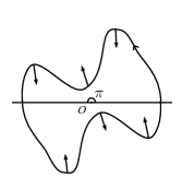
Figure 1.2. CSF on a double cover of $C_{\pi}$

The maximum principle of parabolic equations shows that the CSF remains embedded and hence by the symmetry of the lifting, the CSF can not touch the cone tip in $C_{\pi}$.

For conic Riemann surfaces, we prove that CSF can not touch the cone tip if the cone angle is between $0$ and $\pi$.

Theorem 1.5.

Let $M$ be a conic Riemann surface. Suppose that $\{\Gamma_{t}\}_{t\in[0,T)}$ is a curve shortening flow starting with a smooth closed embedded curve $\Gamma_{0}$. Assume $T<\infty$. If $p\in M$ is a conic singularity with cone angle less than or equal to $\pi$, then either $\lim_{t\to T}\Gamma_{t}=p,$ or the distance function $\mathbf{d}(\Gamma_{t},p)>c>0$ for all $t\in(0,T)$.

The conic singularities on surfaces are ambient singularities of CSF. By Theorem 1.5, CSF in some sense can detect ambient singularities. This is quite different from $\mathbb{R}^{2}$ or smooth surfaces. In $\mathbb{R}^{2}$, a priori, it is not easy to forecast the precise ending point of a CSF. We intend to study the mean curvature flow with ambient singularities in higher dimensions. It is reasonable to expect mean curvature flow to detect ambient singularities in a similar fashion.

We organize the paper as follows: In Section 2, we provide some background and historic notes of CSF. We sketch the idea of Huisken’s proof of Gage-Hamilton-Grayson Theorem in $\mathbb{R}^{2}$. In Section 3, we collect some formulae for the distance functions on surfaces. In Section 4, we prove Theorem 1.1. In Section 5, we study Type I singularities on surfaces. In Section 6, we provide an introduction on conic Riemann surfaces and discuss the construction of a double branched cover. In Section 7, we prove Theorem 1.5.

Acknowledgments

I would like to thank Jian Song for introducing me this topic. I want to thank Hao Fang, Jian Song, and James Dibble for discussions and comments. I thank Marc Troyanov for pointing out a flaw in my original proof. I want to thank Shanghai Jiaotong University and Mijia Lai for hospitality during my visit there.

2. Backgrounds and historical notes

Let $(M,g)$ be a compact Riemann surface. The curve shortening flow $\{\Gamma_{t}\}$ is parametrized by:

$$X :S^{1}\times[0,T)\to M,$$

where $X$ evolves under the governing equation:

$$\frac{\partial}{\partial t}X(u,t)=k\boldsymbol{n}.$$

Here $k$ is the geodesic curvature and $\boldsymbol{n}$ is the normal vector at $X(u,t)$ such that the orientation $\{\frac{\partial}{\partial u}X,\boldsymbol{n}\}$ agrees with the preferred orientation on $M$. The total length $L(t)$ of $\Gamma_{t}$ is decreasing along the CSF [Gra89]. In fact, let $s$ be the length parameter such that $L(t)=\int_{\Gamma_{t}}ds$. Then,

(2.1) $$\frac{d}{dt}ds =\frac{\partial}{\partial t}\langle\frac{\partial X}{\partial u},\frac{\partial X}{\partial u}\rangle^{\frac{1}{2}}du=\|\frac{\partial X}{\partial u}\|^{-1}\langle\frac{\partial^{2}X}{\partial u\partial t},\frac{\partial X}{\partial u}\rangle du$$

$$=\langle\frac{\partial^{2}X}{\partial t\partial u},\frac{\partial X}{\partial s}\rangle du=\langle\frac{\partial}{\partial u}(k\boldsymbol{n}),\frac{\partial X}{\partial s}\rangle du$$

$$=\left(\frac{\partial}{\partial s}\langle k\boldsymbol{n},\frac{\partial X}{\partial s}\rangle\right)ds-\langle k\boldsymbol{n},\frac{\partial^{2}X}{\partial s^{2}}\rangle ds$$

$$=-\langle k\boldsymbol{n},k\boldsymbol{n}\rangle ds=-k^{2}ds.$$

Hence,

$$\frac{d}{dt}L(t)=-\int_{\Gamma_{t}}k^{2}ds.$$

Therefore, CSF can be view as a gradient flow of the total length functional.

Next, we recall two exact solutions of CSF.

Example 2.1.

(Shrinking round circle). In $\mathbb{R}^{2}$, suppose that $\Gamma_{t}$ are circles of radius $R(t)=\sqrt{R_{0}^{2}-2t}$ with center at $0$ . Then $\{\Gamma_{t}\}$ is a CSF for $t\in(-\infty,R_{0}^{2}/2)$. Clearly, $\{\Gamma_{t}\}$ is a self-similar shrinking solution.

Example 2.2.

(Grim Reaper). Let $\Gamma_{t}={\rm graph\ of}\{-\log\cos x\}+t\subset\mathbb{R}^{2}$ for $x\in(-\pi/2,\pi/2)$ and $t\in(-\infty,\infty)$. It is a translating self-similar solution

Historically, Gage and Hamilton [GH86] first obtained the shrinking results of CSF for convex planar curves. They proved that under CSF, closed embedded convex curves in $\mathbb{R}^{2}$ shrink to a round point. Grayson in[Gra87] proved the same results for general curves without requiring convexity. In fact, he proved that any closed embedded curve will eventually become convex and shrink to a point. Grayson’s proof was quite delicate in which he combined different types of analysis to deal with various geometric configurations.

CSF is a special case of general mean curvature flow (MCF), which by its name means embedded hypersurfaces evolving by their mean curvature vectors. It has short time existence as long as the geodesic curvature stays uniformly bounded. Therefore, CSF exists and keeps embedded in a time interval $[0,T)$. When the geodesic curvature $k\to\infty$ as $t\to T$, singularities will happen.

A different proof of Gage-Hamilton-Grayson for planar curves is based on analyzing the behavior at the first time singularities [Hui90, Hui98, Alt91, Ang91]. See [Has16] for an excellent exposition. Let $T$ be the time when the first singularity happens. The singularities of CSF can be classified into 2 types :

• Type I singularities: $\sup_{\Gamma_{t}}|k|\leq\frac{C}{\sqrt{T-t}}$.

• Type II singularities: $\limsup_{t\to T}\left((T-t)\sup_{\Gamma_{t}}|k|^{2}\right)=\infty.$

To deal with Type I singularities, Huisken defined the backward heat kernel [Hui90]:

$$\rho_{x_{0}}(x,t)=\left(4\pi\left(t_{0}-t\right)\right)^{-1/2}e^{-\frac{\left|x-x_{0}\right|^{2}}{4\left(t_{0}-t\right)}}.\mathbf{}$$

He showed

(2.2) $$\frac{d}{dt}\int_{\Gamma_{t}}\rho_{x_{0}}ds=-\int_{\Gamma_{t}}\left|k+\frac{\langle X,\boldsymbol{n}\rangle}{2\left(t_{0}-t\right)}\right|^{2}\rho_{x_{0}}ds<0.$$

After a rescaling, Type I singularities converge to some ancient CSF and by (2.2), they happen to be self-similar shrinking solutions of CSF, which can only be round circles[AL86, Ang91]. Similar results can be derived for MCF on $\mathbb{R}^{n}$ [Hui90], except for MCF, more self-similar shrinking solutions exist. Hamilton [Ham93] generalized Huisken’s formula to manifolds assuming some additional geometric conditions. We will establish a localized backward heat kernel formula on surfaces to study Type I singularities in Section 5.

A big difference between CSF and higher dimensional MCF is the non-existence of Type II singularities. For CSF of a simple closed embedded curve on $\mathbb{R}^{2}$, Type II singularities can never happen while they can happen in general for MCF. The absence of Type II singularities of CSF on $\mathbb{R}^{2}$ can be seen using Huisken’s comparison function:

$$R_{H}(t):=\sup_{x,y}\frac{L(t)}{\pi d(x,y,t)}\sin\left(\frac{\pi l(x,y,t)}{L(t)}\right).$$

Huisken proved that for embedded curves $R_{H}(t)$ is non-increasing and has lower bound $1$ which can be achieved only by round circles [Hui98]. To rule out Type II singularities, we can perform Type II blow-up by Altschuler [Alt91] and the limit converges to a grim reaper by Hamilton’s Harnack estimate [Ham95]. However, grim reaper apparently has an unbounded ratio between intrinsic and extrinsic distance which implies that $R_{H}(t)$ is unbounded. This contradicts the monotonicity of $R_{H}(t)$.

Once Type II singularities are excluded, it is clear that the first time singularity can only be Type I and hence a round point. Therefore, the Gage-Hamilton-Grayson theorem on $\mathbb{R}^{2}$ is proved. See details in [Hui98].

3. Distance Variation Formulae.

In this section, we present the distance variation formulae along a geodesic connecting two points on a given curve shortening flow. Many of the formulae have been derived in [Gag90, Gra89]. We collect them for completeness.

Let $X(u,t)$ be a CSF on a Riemann surface as in Section 2. Let $\gamma$ be the shortest geodesic connecting $X(u_{1},t)$ and $X(u_{2},t)$. Let $d$ be the length of $\gamma$. Parametrize $\gamma(\alpha)$ such that

$$\dot{\gamma}=\frac{d}{d\alpha}\gamma,|\dot{\gamma}|=d.$$

By this parametrization, $\gamma(0)=X(u_{1},t)$ and $\gamma(1)=X(u_{2},t)$. Pick a parallel orthonormal frame $\boldsymbol{\tau},\boldsymbol{\nu}$ along the geodesic such that

$$\boldsymbol{\tau}=\frac{\dot{\gamma}}{|\dot{\gamma}|},\boldsymbol{\nu}\perp\boldsymbol{\tau},$$

and $(\boldsymbol{\tau},\boldsymbol{\nu})$ agrees with the preferred orientation on the surface. We will use $\dot{\gamma}_{i},k_{i},\boldsymbol{n}_{i},\boldsymbol{\tau}_{i},\boldsymbol{\nu}_{i}$ respectively to represent $\dot{\gamma},k,\boldsymbol{n},\boldsymbol{\tau},\boldsymbol{\nu}$ evaluated at $X(u_{i},t)$, for $i=1,2$. Let $U_{i}(\alpha)$, $i=1,2$ be the Jacobi field along $\gamma$ such that

$$\begin{cases}U_{1}(0)=\frac{\partial}{\partial u_{1}}X(u_{1},t),\\ U_{1}(1)=0,\end{cases}\quad\begin{cases}U_{2}(0)=0,\\ U_{2}(1)=\frac{\partial}{\partial u_{2}}X(u_{2},t).\end{cases}$$

Let $\boldsymbol{T}_{i}$ be the unit tangent vector at $X(u_{i},t)$. Extend $\boldsymbol{T}_{i}$ to a Jacobi field $\tilde{\boldsymbol{T}_{i}}$ such that $\tilde{\boldsymbol{T}}_{i}=\boldsymbol{T}_{i}$ at $X(u_{i},t)$ and equals $0$ at the other end. Let $W(\alpha)$ be the Jacobi field along $\gamma$ such that

$$W(0)=k_{1}\boldsymbol{n}_{1},W(1)=k_{2}\boldsymbol{n}_{2}.$$

Let $F(u_{1},u_{2},t)=\int_{0}^{1}|\dot{\gamma}|d\alpha$ be the distance.

$$F_{t} =\int_{0}^{1}|\dot{\gamma}|_{t}d\alpha=\int_{0}^{1}\frac{\langle\dot{\gamma},\nabla_{W}\dot{\gamma}\rangle}{|\dot{\gamma}|}d\alpha$$

$$=\frac{1}{d}\int_{0}^{1}\langle\dot{\gamma},\nabla_{\dot{\gamma}}W\rangle d\alpha=\frac{1}{d}\int_{0}^{1}\frac{\partial}{\partial\alpha}\langle\dot{\gamma},W\rangle d\alpha$$

$$=\frac{1}{d}\langle\dot{\gamma}_{2},k_{2}\boldsymbol{n}_{2}\rangle-\frac{1}{d}\langle\dot{\gamma}_{1},k_{1}\boldsymbol{n}_{1}\rangle.$$

Similarly,

$$F_{u_{1}}=\frac{1}{d}\int_{0}^{1}\text{$\frac{\partial}{\partial\alpha}\langle\dot{\gamma},U_{1}\rangle d\alpha=-\frac{1}{d}\langle\dot{\gamma}_{1},U_{1}\rangle,F_{u_{2}}=\frac{1}{d}\langle\dot{\gamma}_{2},U_{2}\rangle.$}$$

With arc-length parameterization, we have

(3.1) $$F_{s_{1}}=-\frac{1}{d}\langle\dot{\gamma}_{1},\boldsymbol{T}_{1}\rangle|_{X(u_{1},t)},F_{s_{2}}=\frac{1}{d}\langle\dot{\gamma}_{2},\boldsymbol{T}_{2}\rangle|_{X(u_{2},t)}.$$

Calculate the second order derivatives:

$$(F_{s_{1}})_{u_{1}} =-\frac{\partial}{\partial u_{1}}(\frac{1}{d}\langle\dot{\gamma}_{1},\boldsymbol{T}_{1}\rangle)$$

$$=-\frac{|U_{1}(0)|\langle\dot{\gamma}_{1},\boldsymbol{T}_{1}\rangle^{2}}{d^{3}}-\frac{1}{d}\langle\nabla_{U_{1}}\dot{\gamma}_{1},\boldsymbol{T}_{1}\rangle-\frac{1}{d}\langle\dot{\gamma}_{1},\nabla_{U_{1}}\boldsymbol{T}_{1}\rangle$$

$$=\frac{|U_{1}(0)|}{d}\left(-\frac{\langle\dot{\gamma}_{1},\boldsymbol{T}_{1}\rangle^{2}}{d^{2}}-\langle\nabla_{\dot{\gamma}_{1}}\tilde{\boldsymbol{T}}_{1},\boldsymbol{T}_{1}\rangle-\langle\dot{\gamma}_{1},\nabla_{\tilde{\boldsymbol{T}}_{1}}\boldsymbol{T}_{1}\rangle\right).$$

Let

$$\mathcal{K}:M\to\mathbb{R}$$

be the Gaussian curvature of $M$. Let $J_{1}(\alpha),J_{2}(\alpha)$ be the solutions of

(3.2) $$J_{1}(1) =0,J_{1}^{\prime}(1)=-d,J_{1}^{\prime\prime}(\alpha)+d^{2}\mathcal{K}(\gamma(\alpha))J_{1}(\alpha)=0,$$

$$J_{2}(0) =0,J_{2}^{\prime}(0)=-d,J_{2}^{\prime\prime}(\alpha)+d^{2}\mathcal{K}(\gamma(\alpha))J_{2}(\alpha)=0.$$

Then, we can write down the Jacobi field $\tilde{\boldsymbol{T}}_{1}$ and its derivative:

(3.3) $$\tilde{\boldsymbol{T}}_{1}(\alpha) =\langle\boldsymbol{T}_{1},\boldsymbol{\tau}_{1}\rangle(1-\alpha)\boldsymbol{\tau}+\langle\boldsymbol{T}_{1},\boldsymbol{\nu}_{1}\rangle\frac{J_{1}(\alpha)}{J_{1}(0)}\boldsymbol{\nu},$$

$$\nabla_{\dot{\gamma}}\tilde{\boldsymbol{T}}_{1}|_{\alpha=0} =-\langle\boldsymbol{T}_{1},\boldsymbol{\tau}_{1}\rangle\boldsymbol{\tau}_{1}+\langle\boldsymbol{T}_{1},\boldsymbol{\nu}_{1}\rangle\frac{J^{\prime}_{1}(0)}{J_{1}(0)}\boldsymbol{\nu}_{1}.$$

Hence, the second variation formula shows

$$F_{s_{1}s_{1}} =\frac{1}{d}\left(-\frac{\langle\dot{\gamma}_{1},\boldsymbol{T}_{1}\rangle^{2}}{d^{2}}+\langle\boldsymbol{T}_{1},\boldsymbol{\tau}_{1}\rangle^{2}-\frac{J_{1}^{\prime}(0)}{J_{1}(0)}\langle\boldsymbol{T}_{1},\boldsymbol{\nu}_{1}\rangle^{2}-\langle\dot{\gamma}_{1},k_{1}\boldsymbol{n}_{1}\rangle\right)$$

$$=-\frac{1}{d}\frac{J_{1}^{\prime}(0)}{J_{1}(0)}\langle\boldsymbol{T}_{1},\boldsymbol{\nu}_{1}\rangle^{2}-\langle\frac{\dot{\gamma}_{1}}{d},k_{1}\boldsymbol{n}_{1}\rangle.$$

Note $\boldsymbol{T}_{1}=\langle\boldsymbol{T}_{1},\boldsymbol{\tau}_{1}\rangle\boldsymbol{\tau}_{1}+\langle\boldsymbol{T}_{1},\boldsymbol{\nu}_{1}\rangle\boldsymbol{\nu}_{1}.$ By parallel transport, we can extend $\boldsymbol{T}_{1}$ such that

$$\bar{\boldsymbol{T}}_{1}(\alpha)=\langle\boldsymbol{T}_{1},\boldsymbol{\tau}_{1}\rangle\boldsymbol{\tau}(\alpha)+\langle\boldsymbol{T}_{1},\boldsymbol{\nu}_{1}\rangle\boldsymbol{\nu}(\alpha).$$

Notice that

$$\langle\dot{\gamma}(\alpha),\bar{\boldsymbol{T}}_{1}(\alpha)\rangle =\langle\dot{\gamma}_{1},\boldsymbol{T}_{1}\rangle|_{X(u_{1},t)}$$

$$=\langle\dot{\gamma}_{2},\bar{\boldsymbol{T}}_{1}(1)\rangle|_{X(u_{2},t)}.$$

Therefore, we can calculate the mixed derivative

(3.4) $$F_{s_{1}s_{2}} =-\left(\frac{\partial}{\partial s_{2}}\frac{1}{d}\right)\langle\dot{\gamma},\boldsymbol{T}_{1}\rangle-\frac{1}{d}\nabla_{\tilde{\boldsymbol{T}}_{2}}\langle\dot{\gamma},\bar{\boldsymbol{T}}_{1}\rangle|_{X(u_{2},t)}$$

$$=\frac{1}{d^{3}}\langle\dot{\gamma}_{1},\boldsymbol{T}_{1}\rangle|_{X(u_{1},t)}\langle\dot{\gamma}_{2},\boldsymbol{T}_{2}\rangle|_{X(u_{2},t)}-\frac{1}{d}\langle\boldsymbol{T}_{1},\boldsymbol{\tau}_{1}\rangle\langle\boldsymbol{T}_{2},\boldsymbol{\tau}_{2}\rangle$$

$$\ -\frac{J_{2}^{\prime}(1)}{d\cdot J_{2}(1)}\langle\boldsymbol{T}_{1},\boldsymbol{\nu}_{1}\rangle\langle\boldsymbol{T}_{2},\boldsymbol{\nu}_{2}\rangle-\frac{1}{d}\langle\dot{\gamma},\nabla_{\tilde{\boldsymbol{T}}_{2}}\bar{\boldsymbol{T}}_{1}\rangle|_{X(u_{2},t)}.$$

We compute

(3.5) $$\frac{\partial}{\partial\alpha}\langle\dot{\gamma},\nabla_{\tilde{\boldsymbol{T}}_{2}}\bar{\boldsymbol{T}}_{1}\rangle =\langle\dot{\gamma},\nabla_{\dot{\gamma}}\nabla_{\tilde{\boldsymbol{T}}_{2}}\bar{\boldsymbol{T}}_{1}\rangle$$

$$=\langle{\rm Rm}(\dot{\gamma},\tilde{\boldsymbol{T}}_{2})\bar{\boldsymbol{T}}_{1},\dot{\gamma}\rangle+\langle\dot{\gamma},\nabla_{\tilde{\boldsymbol{T}}_{2}}\nabla_{\dot{\gamma}}\bar{\boldsymbol{T}}_{1}\rangle$$

$$=-\langle{\rm Rm}(\dot{\gamma},\tilde{\boldsymbol{T}}_{2})\dot{\gamma},\bar{\boldsymbol{T}}_{1}\rangle$$

$$=-\langle\nabla_{\dot{\gamma}}\nabla_{\dot{\gamma}}\tilde{\boldsymbol{T}}_{2},\bar{\boldsymbol{T}}_{1}\rangle.$$

Here, we have used the fact that $\nabla_{\dot{\gamma}}\nabla_{\dot{\gamma}}\tilde{\boldsymbol{T}}_{2}-{\rm Rm}(\dot{\gamma},\tilde{\boldsymbol{T}}_{2})\dot{\gamma}=0$, where ${\rm Rm}(X,Y)$ is the curvature tensor $[\nabla_{X},\nabla_{Y}]-\nabla_{[X,Y]}$. Note $\tilde{\boldsymbol{T}}_{2}|_{\alpha=0}=0$. Thus we have

(3.6) $$\frac{1}{d}\langle\dot{\gamma},\nabla_{\tilde{\boldsymbol{T}}_{2}}\bar{\boldsymbol{T}}_{1}\rangle|_{X(u_{2},t)} =\frac{1}{d}\int_{0}^{1}\frac{\partial}{\partial\alpha}\langle\dot{\gamma},\nabla_{\tilde{\boldsymbol{T}}_{2}}\bar{\boldsymbol{T}}_{1}\rangle d\alpha=-\frac{1}{d}\int_{0}^{1}\langle\nabla_{\dot{\gamma}}\nabla_{\dot{\gamma}}\tilde{\boldsymbol{T}}_{2},\bar{\boldsymbol{T}}_{1}\rangle d\alpha$$

$$=-\frac{1}{d}\int_{0}^{1}\frac{\partial}{\partial\alpha}\langle\nabla_{\dot{\gamma}}\tilde{\boldsymbol{T}}_{2},\bar{\boldsymbol{T}}_{1}\rangle d\alpha=-\frac{1}{d}\langle\nabla_{\dot{\gamma}}\tilde{\boldsymbol{T}}_{2},\bar{\boldsymbol{T}}_{1}\left.\rangle\right|_{\alpha=0}^{\alpha=1}$$

$$=-\frac{1}{d}\langle\langle\boldsymbol{T}_{2},\boldsymbol{\tau}_{2}\rangle\boldsymbol{\tau}+\langle\boldsymbol{T}_{2},\boldsymbol{\nu}_{2}\rangle\frac{J_{2}^{\prime}(\alpha)}{J_{2}(1)}\boldsymbol{\nu},\bar{\boldsymbol{T}}_{1}\left.\rangle\right|_{\alpha=0}^{\alpha=1}$$

$$=-\langle\boldsymbol{T}_{2},\boldsymbol{\nu}_{2}\rangle\langle\boldsymbol{T}_{1},\boldsymbol{\nu}_{1}\rangle\frac{J_{2}^{\prime}(1)-J_{2}^{\prime}(0)}{d\cdot J_{2}(1)}.$$

Therefore, by (3.4) and (3.6), we have

$$F_{s_{1}s_{2}}=-\frac{J_{2}^{\prime}(0)}{d\cdot J_{2}(1)}\langle\boldsymbol{T}_{1},\boldsymbol{\nu}_{1}\rangle\langle\boldsymbol{T}_{2},\boldsymbol{\nu}_{2}\rangle.$$

Similarly,

$$F_{s_{2}s_{1}}=\frac{J_{1}^{\prime}(1)}{d\cdot J_{1}(0)}\langle\boldsymbol{T}_{1},\boldsymbol{\nu}_{1}\rangle\langle\boldsymbol{T}_{2},\boldsymbol{\nu}_{2}\rangle.$$

Note

(3.7) $$\frac{J_{1}^{\prime}(1)}{J_{1}(0)}=-\frac{J_{2}^{\prime}(0)}{J_{2}(1)}.$$

We collect the computations above in the following lemma:

Lemma 3.1.

Suppose that $X(s,t)$ is parametrized by length on the first variable. Suppose that $p_{1}=X(s_{1},t)$ and $p_{2}=X(s_{2},t)$ are inside a disk with radius smaller than the injectivity radius. Let $\gamma$ be the shortest geodesic connecting $p_{1},p_{2}$. Let $F(s_{1},s_{2},t)$ be the length of $\gamma$. Then

(3.8) $$F_{t} =\langle\boldsymbol{\tau}_{2},k_{2}\boldsymbol{n}_{2}\rangle-\langle\boldsymbol{\tau}_{1},k_{1}\boldsymbol{n}_{1}\rangle,$$

$$F_{s_{1}} =-\langle\boldsymbol{\tau}_{1},\boldsymbol{T}_{1}\rangle,F_{s_{2}}=\langle\boldsymbol{\tau}_{2},\boldsymbol{T}_{2}\rangle,$$

$$F_{s_{1}s_{1}} =-\frac{1}{d}\frac{J_{1}^{\prime}(0)}{J_{1}(0)}\langle\boldsymbol{T}_{1},\boldsymbol{\nu}_{1}\rangle^{2}-\langle\boldsymbol{\tau}_{1},k_{1}\boldsymbol{n}_{1}\rangle,$$

$$F_{s_{2}s_{2}} =\frac{1}{d}\frac{J_{2}^{\prime}(1)}{J_{2}(1)}\langle\boldsymbol{T}_{2},\boldsymbol{\nu}_{2}\rangle^{2}+\langle\boldsymbol{\tau}_{2},k_{2}\boldsymbol{n}_{2}\rangle,$$

$$F_{s_{1}s_{2}} =F_{s_{2}s_{1}}=\frac{1}{d}\frac{J_{1}^{\prime}(1)}{J_{1}(0)}\langle\boldsymbol{T}_{1},\boldsymbol{\nu}_{1}\rangle\langle\boldsymbol{T}_{2},\boldsymbol{\nu}_{2}\rangle.$$

In order to obtain estimates using Gaussian curvature bound, we will need Rauch comparison principle [Car92] on Jacobi fields:

Lemma 3.2.

Suppose that the curvature of the Riemann surface is bounded, i.e.

$$K_{M}=\sup_{M}|\mathcal{K}|<\infty.$$

Let $J_{1}(\alpha)$ be defined by

$$J_{1}(1)=0,J_{1}^{\prime}(1)=-d,J_{1}^{\prime\prime}(\alpha)+d^{2}\mathcal{K}(\gamma(\alpha))J_{1}(\alpha)=0.$$

Then, by Rauch comparison principle [Car92],

$$|J_{1}(\alpha)|\leq\frac{1}{\sqrt{K_{M}}}\sinh(d\sqrt{K_{M}}(1-\alpha))=d(1-\alpha)+O(d^{3}),$$

for $0<\alpha<1$. Moreover,

(3.9) $$|J_{1}^{\prime}(\alpha)-J_{1}^{\prime}(1)| =d^{2}|\int_{\alpha}^{1}\mathcal{K}(\gamma(t))J_{1}(t)dt|\leq K_{M}d^{3}(1-\alpha)+O(d^{5}).$$

So there exists a $\delta_{0}=\delta_{0}(K_{M})$ such that if $d<\delta_{0}$ then

(3.10) $$J_{1}^{\prime}(\alpha) \leq-d+2d^{3}K_{M},$$

$$J_{1}(0) \geq d-2d^{3}K_{M}>\frac{1}{2}d.$$

4. Comparison function with exponential decay

In this section, we introduce our new comparison function for CSF on surfaces. By Gage [Gag90], in a local neighborhood away from the singularities of CSF, the distance of two distinct points decreases at most exponentially. Inspired by [Gag90, Hui98], we define a suitable comparison function:

$$R(t)=\sup_{x,y}\frac{L(t)e^{-Kt}}{\pi d(x,y,t)}\sin\left(\frac{\pi l(x,y,t)}{L(t)}\right).$$

If Type II singularity happens in finite time, $R(t)\to\infty$ locally, as was explained in Section 2. Thus, if we want to prove that Type II singularities do not occur, it is sufficient to prove that $R(t)$ is bounded.

Theorem 4.1.

Let $d_{M}$ be the injectivity radius and $K_{M}=\sup_{M}|\mathcal{K}|$ be the Gaussian curvature bound of $M$. Suppose that the curve shortening flow exists in the time period $[0,T)$. There exists a constant $K=K(d_{M},K_{M})$ such that $R(t)$ is bounded by a constant $C(R(0),d_{M},K_{M})$ .

Proof.

Note that $L(t)$ is decreasing. Hence, $L(t)<L(0)$. The $\sin$ part is clearly bounded.

We now argue by contradiction. Suppose that

(4.1) $$\limsup_{t\to T}R(t)=\infty.$$

Pick $d_{0}=\frac{1}{2}\min\{d_{M},\delta_{0}\}$ where $\delta_{0}$ is defined in Lemma 3.2. If $d(x,y,t)>d_{0}$, then $R(t)\leq\frac{L_{0}}{\pi d_{0}}$. Fix a large $N$ such that $N>\max\{\frac{L(0)}{\pi d_{0}},R(0),2\}$ . Let

(4.2) $$Z_{N}(x,y,t)=Nd(x,y,t)-\frac{L(t)}{\pi}\sin\left(\frac{\pi l(x,y,t)}{L(t)}\right)e^{-Kt}.$$

Then, by (4.1), there is a $\bar{t}$ such that for any $0<t<\bar{t}$ , $Z_{N}(x,y,t)>0$ for all $x,y$, $Z_{N}(x,y,\bar{t})\geq 0$ for all $x,y$ and $Z_{N}(\bar{x},\bar{y},\bar{t})=0$ for some $\bar{x},\bar{y}$. We can parametrize the curve $X(\cdot,\bar{t})$ by length with positive orientation such that

$$0\leq l=y-x\leq\frac{L}{2}.$$

By the choice of $N$, we see $d(\bar{x},\bar{y},\bar{t})<\frac{d_{M}}{2}$ . Hence, $d(x,y,t)$ is smooth around $(\bar{x},\bar{y},\bar{t})$. Since $\sin\frac{l\pi}{L}$ is smooth even when $l=\frac{1}{2}L$, $Z_{N}$ is smooth in a neighborhood of $(\bar{x},\bar{y},\bar{t})$. Let

$$p_{1}=X(\bar{x},\bar{t}),p_{2}=X(\bar{y},\bar{t}).$$

We can then connect $X(\bar{x},\bar{t})$ and $X(\bar{y},\bar{t})$ by a shortest geodesic

$$\gamma:[0,1]\to M,\gamma(0)=X(\bar{x},\bar{t}),\gamma(1)=X(\bar{y},\bar{t}).$$

with constant speed $\|\dot{\gamma}\|=d(\bar{x},\bar{y},\bar{t})$. By Lemma 3.1, compute the first variation:

(4.3) $$Z_{N}(x,y,t) =Nd(x,y,t)-\frac{L(t)}{\pi}\sin\left(\frac{\pi l}{L}\right)e^{-Kt},$$

$$\frac{\partial}{\partial x}Z_{N} =-N\langle\boldsymbol{\tau}_{1},\boldsymbol{T}_{1}\rangle+\cos\left(\frac{\pi l}{L}\right)e^{-Kt},$$

$$\frac{\partial}{\partial y}Z_{N} =N\langle\boldsymbol{\tau}_{2},\boldsymbol{T}_{2}\rangle-\cos\left(\frac{\pi l}{L}\right)e^{-Kt}.$$

Second order derivatives are given by

(4.4) $$\frac{\partial^{2}}{\partial x^{2}}Z_{N} =-\frac{N}{d}\frac{J_{1}^{\prime}(0)}{J_{1}(0)}\langle\boldsymbol{T}_{1},\boldsymbol{\nu}_{1}\rangle^{2}-N\langle\boldsymbol{\tau}_{1},k_{1}\boldsymbol{n}_{1}\rangle+\frac{\pi e^{-Kt}}{L(t)}\sin\frac{\pi l(x,y,t)}{L(t)},$$

$$\frac{\partial^{2}}{\partial y^{2}}Z_{N} =\frac{N}{d}\frac{J_{2}^{\prime}(1)}{J_{2}(1)}\langle\boldsymbol{T}_{2},\boldsymbol{\nu}_{2}\rangle^{2}+N\langle\boldsymbol{\tau}_{2},k_{2}\boldsymbol{n}_{2}\rangle+\frac{\pi e^{-Kt}}{L(t)}\sin\frac{\pi l(x,y,t)}{L(t)},$$

$$\frac{\partial^{2}}{\partial x\partial y}Z_{N} =\frac{N}{d}\frac{J_{1}^{\prime}(1)}{J_{1}(0)}\langle\boldsymbol{T}_{1},\boldsymbol{\nu}_{1}\rangle\langle\boldsymbol{T}_{2},\boldsymbol{\nu}_{2}\rangle-\pi L(t)^{-1}\sin\frac{\pi l(x,y,t)}{L(t)}e^{-Kt}.$$

By (2.1), we have

$$\frac{d}{dt}l(x,y,t) =-\int_{x}^{y}k^{2}ds,$$

$$\frac{d}{dt}L(t) =-\int_{S^{1}}k^{2}ds.$$

Compute $t$ derivative:

(4.5) $$\frac{\partial}{\partial t}Z_{N} =N\langle\boldsymbol{\tau}_{2},k_{2}\boldsymbol{n}_{2}\rangle-N\langle\boldsymbol{\tau}_{1},k_{1}\boldsymbol{n}_{1}\rangle+Ke^{-Kt}\frac{L(t)}{\pi}\sin\left(\frac{\pi l}{L}\right)$$

$$+e^{-Kt}\left\{\left(\frac{1}{\pi}\sin\frac{\pi l}{L}-\frac{l}{L}\cos\frac{\pi l}{L}\right)\int_{S^{1}}k^{2}du+\cos\left(\frac{\pi l}{L}\right)\int_{x}^{y}k^{2}ds\right\}.$$

At $(\bar{x},\bar{y},\bar{t})$, we have that

(4.6) $$Nd =\frac{L}{\pi}\sin\left(\frac{\pi l}{L}\right)e^{-K\bar{t}}.$$

Since $Z_{N}$ achieves minimum at $(\bar{x},\bar{y},\bar{t})$, by Lemma 3.1,

(4.7) $$\frac{\partial}{\partial x}Z_{N} =\frac{\partial}{\partial y}Z_{N}=0,$$

(4.8) $$0<\langle\boldsymbol{\tau}_{i},\boldsymbol{T}_{i}\rangle =\frac{1}{N}\cos\left(\frac{\pi l}{L}\right)e^{-K\bar{t}}\leq\frac{1}{N}.$$

We denote $\theta=\arccos\langle\boldsymbol{\tau}_{1},\boldsymbol{T}_{1}\rangle$. Equation (4.8) implies either $\langle\boldsymbol{T}_{1},\boldsymbol{\nu}_{1}\rangle=\langle\boldsymbol{T}_{2},\boldsymbol{\nu}_{2}\rangle$ or $\langle\boldsymbol{T}_{1},\boldsymbol{\nu}_{1}\rangle=-\langle\boldsymbol{T}_{2},\boldsymbol{\nu}_{2}\rangle$. We consider each case separately.

Case 1. $\langle\boldsymbol{T}_{1},\boldsymbol{\nu}_{1}\rangle=\langle\boldsymbol{T}_{2},\boldsymbol{\nu}_{2}\rangle$. By Lemma 3.2, we have

$$|J_{i}^{\prime}(0)-J_{i}^{\prime}(1)|\leq C_{1}d^{3},|J_{1}(0)|\geq\frac{1}{2}d,$$

where $C_{1}=C_{1}(K_{M})$. Let $K>4C_{1}$ . Define the operator

$$\mathcal{L_{+}:=}\frac{\partial}{\partial t}-\frac{\partial^{2}}{\partial x^{2}}-\frac{\partial^{2}}{\partial y^{2}}+2\frac{\partial^{2}}{\partial x\partial y}.$$

By Lemma 3.2, (4.4) , (4.5) and (4.6)we have

$$\mathcal{L}_{+}Z_{N} |_{(\bar{x},\bar{y},\bar{t})}=\frac{N}{d}\left(\frac{J_{1}^{\prime}(0)-J_{1}^{\prime}(1)}{J_{1}(0)}-\frac{J_{2}^{\prime}(1)-J_{2}^{\prime}(0)}{J_{2}(1)}\right)\langle\boldsymbol{T}_{1},\boldsymbol{\nu}_{1}\rangle^{2}$$

$$+e^{-K\bar{t}}\left\{\left(\frac{1}{\pi}\tan\frac{\pi l}{L}-\frac{l}{L}\right)\cos\frac{\pi l}{L}\int_{S^{1}}k^{2}ds\right.$$

$$\left.+\cos\left(\frac{\pi l}{L}\right)\int_{\bar{x}}^{\bar{y}}k^{2}ds+K\frac{L}{\pi}\sin\frac{\pi l}{L}\right\}$$

$$\geq-4C_{1}Nd+Ke^{-K\bar{t}}\frac{L}{\pi}\sin\frac{\pi l}{L}$$

$$=(K-4C_{1})e^{-K\bar{t}}\frac{L}{\pi}\sin\frac{\pi l}{L}>0.$$

This contradicts with the fact that $Z_{N}(\cdot,\cdot,\bar{t})$ achieves local minimum at $(\bar{x},\bar{y})$.

Case 2. $\langle\boldsymbol{T}_{1},\boldsymbol{\nu}_{1}\rangle=-\langle\boldsymbol{T}_{2},\boldsymbol{\nu}_{2}\rangle.$ We need the following isoperimetric inequality:

$$|\partial\Omega|^{2}\geq 4\pi|\Omega|-K_{M}|\Omega|^{2},$$

for a simply connected region $\Omega$ with piece-wise $C^{1}$ boundary on $M$, see [Oss78]. Then, there exists a $\delta_{1}=\delta_{1}(d_{M},K_{M})$ such that

$$|\partial\Omega|^{2}\geq 2\pi|\Omega|,$$

as long as $\Omega$ is inside a geodesic disk $D_{\delta_{1}}(p)$ such that

$$|D_{\delta_{1}}(p)|<2\pi K_{M}^{-1}.$$

Let $\delta_{M}=\min\{\delta_{1},\frac{1}{2(1+K_{M})}\}$. We will discuss two subcases.

Subcase 2a. We assume $L(\bar{t})\geq\delta_{M}>0.$ Define the operator

$$\mathcal{L_{-}:=}\frac{\partial}{\partial t}-\frac{\partial^{2}}{\partial x^{2}}-\frac{\partial^{2}}{\partial y^{2}}-2\frac{\partial^{2}}{\partial x\partial y}.$$

Since $Z_{N}(\cdot,\cdot,\bar{t})$ attains local minimum at $(\bar{x},\bar{y})$, we have $\mathcal{L}_{-}Z_{N}|_{(\bar{x},\bar{y},\bar{t})}\leq 0$. By Lemma 3.2,

(4.9) $$\mathcal{L_{-}}Z_{N}|_{(\bar{x},\bar{y},\bar{t})}= \frac{N}{d}\left(\frac{J_{1}^{\prime}(0)-J_{1}^{\prime}(1)}{J_{1}(0)}-\frac{J_{2}^{\prime}(1)-J_{2}^{\prime}(0)}{J_{2}(1)}\right)\langle\boldsymbol{T}_{1},\boldsymbol{\nu}_{1}\rangle^{2}$$

$$+e^{-K\bar{t}}\left\{\left(\frac{1}{\pi}\tan\frac{\pi l}{L}-\frac{l}{L}\right)\cos\frac{\pi l}{L}\int_{S^{1}}k^{2}ds\right.$$

$$\left.+\cos\left(\frac{\pi l}{L}\right)\int_{x}^{y}k^{2}ds+K\frac{L}{\pi}\sin\frac{\pi l}{L}-\frac{4\pi}{L}\sin\frac{\pi l}{L}\right\}$$

$$\geq-4C_{1}Nd+Ke^{-K\bar{t}}\frac{L}{\pi}\sin\frac{\pi l}{L}-e^{-K\bar{t}}\frac{4\pi}{L}\sin\frac{\pi l}{L}$$

$$=(K-4C_{1}-\frac{4\pi^{2}}{L^{2}})e^{-K\bar{t}}\frac{L}{\pi}\sin\frac{\pi l}{L}$$

$$\geq(K-4C_{1}-\frac{4\pi^{2}}{\delta_{M}^{2}})e^{-K\bar{t}}\frac{L}{\pi}\sin\frac{\pi l}{L}.$$

If

(4.10) $$K>4C_{1}+\frac{4\pi^{2}}{\delta_{M}^{2}},$$

then $\mathcal{L_{-}}Z_{N}|_{(\bar{x},\bar{y},\bar{t})}>0$ and we have reached a contradiction.

Subcase 2b. We assume $L(\bar{t})<\delta_{M}$. Then, $\Gamma_{\bar{t}}$ is contained in a geodesic disk $D_{\delta_{M}}(p)$ centered at a point $p$ . By Gauss-Bonnet formula,

(4.11) $$\int_{S^{1}}k(u)du+\int_{\Omega_{\bar{t}}}\mathcal{K}(z)d\mu(z)=2\pi,$$

where $\Omega_{\bar{t}}$ is the region enclosed by the curve $X(\cdot,\bar{t})$. We have the isoperimetric inequality

(4.12) $$|\Omega_{\bar{t}}|\leq L^{2}/2\pi.$$

Thus by (4.11) , (4.12) and the fact that $L<\delta_{M}$, we obtain

$$\int_{S^{1}}|k|ds\geq 2\pi-|\Omega_{\bar{t}}|\sup\mathcal{K}\geq 2\pi-L^{2}\frac{K_{M}}{2\pi}>0.$$

By Cauchy-Schwarz inequality, we have

(4.13) $$\int_{S^{1}}k^{2}ds \geq\frac{1}{L}(\int_{S^{1}}|k|ds)^{2}\geq\frac{4\pi^{2}}{L}-2K_{M}L.$$

Now, the shortest geodesic $\gamma$ together with the arc of $X(\cdot,\bar{t})$ from $\bar{x}$ to $\bar{y}$ enclose a region, denoted as $\Omega_{\bar{t}}^{+}$. Note

$$\partial\Omega_{\bar{t}}^{+}=\{X(s,\bar{t}):s\in[\bar{x},\bar{y}]\}\cup\{\gamma(\alpha):\alpha\in[0,1]\}.$$

Clearly, $|\partial\Omega_{\bar{t}}^{+}|\leq 2l$. Two outer angles at $p_{1}$ and $p_{2}$ on $\partial\Omega_{\bar{t}}^{+}$ are both equal to $\pi-\theta$. By Gauss-Bonnet formula and isoperimetric inequality (4.12), we have

$$\int_{\bar{x}}^{\bar{y}}kds =2\pi-\int_{\Omega_{\bar{t}}^{+}}\mathcal{K}(z)d\mu(z)-2(\pi-\theta)$$

$$=2\theta-\int_{\Omega_{\bar{t}}^{+}}\mathcal{K}(z)d\mu(z)$$

(4.14) $$\geq 2\theta-\frac{2K_{M}}{\pi}l^{2}>0.$$

Note that the last inequality $2\theta-\frac{2K_{M}}{\pi}l^{2}>0$ holds since $\cos\theta<\frac{1}{N}$ and

$$\frac{K_{M}}{\pi}l^{2}<\frac{K_{M}}{(1+K_{M})^{2}4\pi}<\frac{\pi}{3}<\arccos\frac{1}{N}.$$

Hence, by Cauchy-Schwarz inequality,

(4.15) $$\int_{\bar{x}}^{\bar{y}}k^{2}ds\geq\frac{1}{l}(2\theta-\frac{2K_{M}}{\pi}l^{2})^{2}\geq\frac{4\theta^{2}}{l}-\frac{8K_{M}\theta l}{\pi}.$$

We have

$$\mathcal{L_{-}}Z_{N}|_{(\bar{x},\bar{y},\bar{t})} =\frac{N}{d}\left(\frac{J_{1}^{\prime}(0)-J_{1}^{\prime}(1)}{J_{1}(0)}-\frac{J_{2}^{\prime}(1)-J_{2}^{\prime}(0)}{J_{2}(1)}\right)\langle\boldsymbol{T}_{1},\boldsymbol{\nu}_{1}\rangle^{2}$$

$$+e^{-K\bar{t}}\left[\frac{KL}{\pi}\sin\frac{\pi l}{L}-\frac{4\pi}{L}\sin\frac{\pi l}{L}+\cos\left(\frac{\pi l}{L}\right)\int_{x}^{y}k^{2}ds\right]$$

$$+e^{-K\bar{t}}\left(\frac{1}{\pi}\sin\frac{\pi l}{L}-\frac{l}{L}\cos\frac{\pi l}{L}\right)\int_{S^{1}}k^{2}ds.$$

In the following, we use $C(K_{M})$ to represent some constants depending only on $K_{M}$. By Lemma 3.2, (4.13) and (4.14), we have

$$0 \geq\mathcal{L}_{-}Z_{N}|_{(\bar{x},\bar{y},\bar{t})}\geq-4C_{1}Nd$$

$$\ \ +e^{-K\bar{t}}\left[\frac{KL}{\pi}\sin\frac{\pi l}{L}-\frac{4\pi}{L}\sin\frac{\pi l}{L}+\cos\left(\frac{\pi l}{L}\right)\int_{x}^{y}k^{2}ds\right]$$

$$\ \ +e^{-K\bar{t}}\left(\frac{1}{\pi}\sin\frac{\pi l}{L}-\frac{l}{L}\cos\frac{\pi l}{L}\right)\left(\frac{4\pi^{2}}{L}-C(K_{M})L\right)$$

$$\geq-4C_{1}Nd+e^{-K\bar{t}}\left(\frac{KL}{\pi}-C(K_{M})L\right)\sin\frac{\pi l}{L}$$

$$\ +e^{-K\bar{t}}\left[\cos\left(\frac{\pi l}{L}\right)\int_{x}^{y}k^{2}ds-\frac{l}{L}\cos\frac{\pi l}{L}\left(\frac{4\pi^{2}}{L}-C(K_{M})L\right)\right].$$

Then, by (4.15) and (4.6),

$$\mathcal{L}_{-}Z_{N}|_{(\bar{x},\bar{y},\bar{t})} \geq-4C_{1}Nd+e^{-K\bar{t}}\left(K-C(K_{M})\right)\frac{L}{\pi}\sin\frac{\pi l}{L}$$

$$\ +e^{-K\bar{t}}\cos\frac{\pi l}{L}\left[4\theta^{2}-\frac{8\theta K_{M}}{\pi}l^{2}-\frac{4\pi^{2}l^{2}}{L^{2}}\right]\frac{1}{l}$$

$$=-4C_{1}Nd+e^{-K\bar{t}}\frac{L}{\pi}\sin\frac{\pi l}{L}\left(K-C(K_{M})-C(K_{M})\frac{4\pi\theta l}{L}\cot\frac{l\pi}{L}\right)$$

$$\ +e^{-K\bar{t}}\cos\frac{\pi l}{L}\left[4\theta^{2}-4\pi^{2}\frac{l^{2}}{L^{2}}\right]\frac{1}{l}$$

$$\geq e^{-K\bar{t}}\left[\frac{L}{\pi}\sin\frac{\pi l}{L}\left(K-C(K_{M})-4C_{1}\right)+\frac{1}{l}\cos\frac{\pi l}{L}\left(4\theta^{2}-4\pi^{2}\frac{l^{2}}{L^{2}}\right)\right].$$

We can pick $K\geq C(K_{M})+4C_{1}$. In order to keep $\mathcal{L}_{-}Z_{N}|_{(\bar{x},\bar{y},\bar{t})}\leq 0$, it forces $4\theta^{2}-4\pi^{2}\frac{l^{2}}{L^{2}}\leq 0$ and hence $\theta\leq\frac{\pi l}{L}$. However, by (4.8)

$$\cos\theta=\frac{e^{-K\bar{t}}}{N}\cos\frac{\pi l}{L}<\cos\frac{\pi l}{L},$$

which is impossible.

By ruling out Case 1 and Case 2, we see that $Z_{N}(\cdot,\cdot,\bar{t})$ can not reach minimum $0$ at $(\bar{x},\bar{y})$, which implies that $Z_{N}(t)>0$ for $t\in[0,T)$. Hence, $R(t)<N$. We have proved the theorem. ∎

A non-existence result for Type II singularities now can be easily derived.

Corollary 4.2.

Embedded simple closed curves can not develop Type II singularities in finite time.

Proof.

By performing Type II blow-ups [Alt91], CSF near the singularity should converge to a grim reaper by Hamilton’s Harnack estimate [Ham95]. However, for a grim reaper, the ratio of intrinsic and extrinsic distance blows up which contradicts Theorem 4.1. ∎

5. Analysis on Type I singularities

In this section, we focus on Type I singularities on Riemann surfaces. The main tool we use here is a localized Huisken’s backward heat kernel monotonicity formula. Fix a point $x_{0}\in M$. Let $x\in\Gamma_{t}$ . We may assume $x=X(0,t)$. Let $\gamma:[0,1]\times(-\epsilon,\epsilon)\to M$ be a family of geodesic such that $\gamma(0,u)=x_{0}$, $\gamma(1,u)=X(u,t)$ and

$$\|\dot{\gamma}\|_{g}=\mathbf{d}_{g}(x_{0},X(t,u)),$$

where $\mathbf{d}_{g}$ is the distance function on $(M,g)$. Here, we use $\dot{\gamma}(\alpha,u)$ to denote $\frac{\partial}{\partial\alpha}\gamma(\alpha,u)$. Let

$$\boldsymbol{T}:=\frac{\partial}{\partial s}=\frac{\partial X}{\partial u}/\|\frac{\partial X}{\partial u}\|_{g}$$

By the first variation formula,

$$\frac{\partial}{\partial s}\|\dot{\gamma}\|_{g}=\frac{1}{\|\dot{\gamma}\|_{g}}\langle\boldsymbol{T},\dot{\gamma}\rangle_{g}.$$

Let $\boldsymbol{\nu}$ be a vector field orthogonal to $\dot{\gamma}$ and parallel along $\gamma$. Let $\mathcal{K}$ be the Gaussian curvature of $(M,g)$. Let $J(\alpha)$ to be a function such that

(5.1) $$\begin{cases}J^{\prime\prime}(\alpha)+\mathbf{d}_{g}^{2}(x_{0},x)\mathcal{K}(\gamma(\alpha,0))J(\alpha)=0,\\ J(0)=0,J^{\prime}(0)=\mathbf{d}_{g}(x_{0},x).\end{cases}$$

Then we can extend $\mathcal{\boldsymbol{T}}$ to be a Jacobi field by setting

$$\mathcal{\boldsymbol{T}}(\gamma(\alpha,0))=\left\langle\mathcal{\boldsymbol{T}},\frac{\dot{\gamma}}{\|\dot{\gamma}\|}\right\rangle_{g}\alpha\frac{\dot{\gamma}(\alpha,0)}{\|\dot{\gamma}\|_{g}}+\left\langle\mathcal{\boldsymbol{T}},\boldsymbol{\nu}\right\rangle_{g}\frac{J(\alpha)}{J(1)}\boldsymbol{\nu}(\alpha).$$

Then $\frac{J(\alpha)\boldsymbol{\nu}(\alpha)}{J(1)}$ will be a Jacobi field along $\gamma(\alpha)$. Therefore, at $x$,

(5.2) $$\nabla_{\mathcal{\boldsymbol{T}}}\dot{\gamma}=\nabla_{\dot{\gamma}}\mathcal{\boldsymbol{T}}=\mathcal{\boldsymbol{T}}+\frac{J^{\prime}(1)-J(1)}{J(1)}\boldsymbol{\nu}.$$

Denote $\mathcal{J}_{x}:=\frac{J^{\prime}(1)-J(1)}{J(1)}$.

Lemma 5.1.

Let $K_{M}=\sup_{x\in M}|\mathcal{K}(x)|$ and $d=\mathbf{d}_{g}(x,x_{0})$. Let $J(\alpha)$ be a solution of (5.1). By Lemma 3.2, if $d<\delta_{0}$, then

(5.3) $$|\mathcal{J}_{x}|\leq C(K_{M})d^{2}.$$

Let $g_{1}=c^{2}g$ and $\tilde{J}(\alpha)$ be a solution of

$$\begin{cases}\tilde{J}^{\prime\prime}(\alpha)+\mathbf{d}_{g_{1}}^{2}(x_{0},x)\mathcal{K}_{g_{1}}(\gamma(\alpha,0))\tilde{J}(\alpha)=0,\\ \tilde{J}(0)=0,\tilde{J}^{\prime}(0)=\mathbf{d}_{g_{1}}(x_{0},x).\end{cases}$$

then $\tilde{J}(\alpha)=cJ(\alpha)$ and

$$\tilde{\mathcal{J}_{x}}:=\frac{\tilde{J}^{\prime}(1)-\tilde{J}(1)}{\tilde{J}(1)}=\mathcal{J}_{x}.$$

Since we are interested in the behavior of CSF near singularities, we consider $t\in[t_{0},T)$ such that $T-1<t_{0}<T$. Define

$$\tau=-\frac{1}{2}\ln(T-t),t\in[t_{0},T).$$

Then, $\tau\in[\tau_{0},\infty)$ for $\tau_{0}=-\frac{1}{2}\ln(T-t_{0})$. Let $d_{M}$ be the injectivity radius of $M$ and let

$$r_{M}=\min\{\delta_{0},\frac{1}{8}d_{M}\}.$$

Let $\eta_{0}(r)$ be a smooth cut-off function such that

$$\eta_{0}(r)=\begin{cases}1&0\leq r<1,\\ 0&r>2,\end{cases}$$

We may assume further that $0\geq\eta^{\prime}_{0}>-2$. Now, We define

$$M_{x_{0}}(x):=\frac{1}{\sqrt{2(T-t)}}\exp\left(-\frac{\mathbf{d}_{g}(x_{0},x)^{2}}{4(T-t)}\right)\eta_{0}\left(\frac{\mathbf{d}_{g}(x_{0},x)^{2}}{4(T-t)\tau^{2}r_{M}^{2}}\right).$$

We call $M_{x_{0}}(x)$ a localized Huisken’s backward heat kernel function.

Definition 5.2.

(Rescaled flow) Let the rescaled pointed manifold $M_{\tau}$ to be the pair $(M,x_{0},g_{\tau})$ with metric

$$g_{\tau}=(2(T-t))^{-1}g=\frac{e^{2\tau}}{2}g.$$

We use $\langle,\rangle_{\tau}$ to denote the inner product under metric $g_{\tau}$. Let $\Gamma_{\tau}=\Gamma_{t}$ such that $t=\frac{1}{2}e^{2\tau}$ but under the metric $g_{\tau}$. Likewise, we define $\sqrt{2}e^{-\tau}ds_{\tau}=ds$, $k_{\tau}=k\sqrt{2}e^{-\tau}$, $\mathbf{d}_{\tau}(\cdot,\cdot)=\text{{d}}_{g_{\tau}}(\cdot,\cdot)$ to be the length form, geodesic curvature and distance function with respect to the metric $g_{\tau}$.

Under metric $g_{\tau}$, we have

$$M_{x_{0}}ds=\exp\left(-\mathbf{d}_{\tau}(x_{0},x)^{2}/2\right)\eta_{0}\left(\frac{\mathbf{d}_{\tau}(x_{0},x)^{2}}{2\tau^{2}r_{M}^{2}}\right)ds_{\tau},$$

Let

$$\rho(x):=\exp\left(-\mathbf{d}_{\tau}(x_{0},x)^{2}/2\right),$$

and

$$\eta(x):=\eta_{0}\left(\frac{\mathbf{d}_{\tau}(x_{0},x)^{2}}{2\tau^{2}r_{M}^{2}}\right)=\eta_{0}\left(\phi_{\tau,x_{0}}(x)\right),$$

where $\phi_{\tau,x_{0}}(x)=\frac{\mathbf{d}_{\tau}(x_{0},x)^{2}}{2\tau^{2}r_{M}}$. Finally, define

$$\mathcal{M}_{\tau}:=\int_{\Gamma_{\tau}}\rho\eta ds_{\tau}.$$

Theorem 5.3.

Suppose that $\sup_{\tau,x}|k_{\tau}(x)|<C(k)<\infty$. Then, there exist constants $C_{1},C_{2}$ depending on $K_{M},r_{M},L(0)$ such that

(5.4) $$\frac{d}{d\tau}\left(p(\tau)\mathcal{M}_{\tau}\right)\leq C_{2}p(\tau)\exp(2\tau-\tau^{2}r_{M}^{2})\tau^{-1},$$

where $p(\tau)=\exp\left(-C_{1}\int_{0}^{\tau}e^{-2y}y^{2}dy\right)$.

Proof.

For $x\in\Gamma_{t}$, we may assume $x=X(0,t)$. Let $\gamma:[0,1]\times(-\epsilon,\epsilon)\to M$ be a family of geodesics such that $\gamma(0,u)=x_{0}$, $\gamma(1,u)=X(u,t)$ and $\|\dot{\gamma}\|_{g}=\mathbf{d}_{g}(x_{0},X(t,u))$. Since $\eta(x)\not=0$ only if $\mathbf{d}_{\tau}(x_{0},x)^{2}\leq 4\tau^{2}r_{M}^{2}$, we may assume

$$\mathbf{d}_{g}^{2}(x_{0},x)\leq 8e^{-2\tau}\tau^{2}r_{M}^{2}\leq d_{M}^{2}.$$

Hence, we can use the first variation formula and obtain

$$\frac{\partial}{\partial\tau}\|\dot{\gamma}\|_{\tau}^{2}=\frac{\partial}{\partial\tau}\left(\frac{1}{2}e^{-2\tau}\|\dot{\gamma}\|_{g}^{2}\right)=\left(\langle\dot{\gamma},k_{\tau}\boldsymbol{n}\rangle_{\tau}+\|\dot{\gamma}\|_{\tau}^{2}\right).$$

By (5.2),

(5.5) $$\frac{\partial}{\partial s_{\tau}}\rho =-\rho\langle\dot{\gamma},\nabla_{\mathcal{\boldsymbol{T}}}\dot{\gamma}\rangle_{\tau}=-\rho\langle\dot{\gamma},\mathcal{\boldsymbol{T}}\rangle_{\tau}.$$

Combining (5.2) and (5.5), we have

(5.6) $$\int_{\Gamma_{\tau}}\rho\eta ds =\int_{\Gamma_{\tau}}\rho\eta\langle\mathcal{\boldsymbol{\boldsymbol{T}}},\mathcal{\boldsymbol{\boldsymbol{T}}}\rangle_{\tau}ds_{\tau}$$

$$=\int_{\Gamma_{\tau}}\rho\eta\langle\mathcal{\boldsymbol{T}},\nabla_{\mathcal{\boldsymbol{T}}}\dot{\gamma}\rangle_{\tau}ds_{\tau}-\int_{\Gamma_{\tau}}\rho\eta\langle\mathcal{\boldsymbol{T}},\mathcal{J}_{x}\boldsymbol{\nu}\rangle_{\tau}ds_{\tau}$$

$$=\int_{\Gamma_{\tau}}\frac{\partial}{\partial s_{\tau}}\left(\rho\eta\langle\mathcal{\boldsymbol{T}},\dot{\gamma}\rangle_{\tau}\right)ds_{\tau}-\int_{\Gamma_{\tau}}\rho\eta\langle\nabla_{\mathcal{\boldsymbol{T}}}\mathcal{\mathcal{\boldsymbol{T}}},\dot{\gamma}\rangle_{\tau}ds_{\tau}-\int_{\Gamma_{\tau}}\langle\mathcal{\boldsymbol{T}},\dot{\gamma}\rangle_{\tau}\eta\frac{\partial}{\partial s_{\tau}}\rho ds_{\tau}$$

$$\ -\int_{\Gamma_{\tau}}\langle\mathcal{\boldsymbol{T}},\dot{\gamma}\rangle_{\tau}\rho\frac{\partial}{\partial s_{\tau}}\eta ds_{\tau}-\int_{\Gamma_{\tau}}\rho\eta\langle\mathcal{\boldsymbol{T}},\mathcal{J}_{x}\boldsymbol{\nu}\rangle_{\tau}ds_{\tau}$$

$$=-\int_{\Gamma_{\tau}}\rho\eta\langle k\boldsymbol{n},\dot{\gamma}\rangle_{\tau}ds_{\tau}+\int_{\Gamma_{\tau}}\rho\eta\langle\mathcal{\boldsymbol{T}},\dot{\gamma}\rangle^{2}ds_{\tau}-\int_{\Gamma_{\tau}}\langle\mathcal{\boldsymbol{T}},\dot{\gamma}\rangle_{\tau}\rho\frac{\partial}{\partial s_{\tau}}\eta ds_{\tau}$$

$$\ -\int_{\Gamma_{\tau}}\rho\eta\langle\mathcal{\boldsymbol{T}},\mathcal{J}_{x}\boldsymbol{\nu}\rangle_{\tau}ds_{\tau}.$$

Since $\sqrt{2}e^{-\tau}ds_{\tau}=ds,$ we have

(5.7) $$\frac{\partial}{\partial\tau}ds_{\tau} =(1-k_{\tau}^{2})ds_{\tau}.$$

Therefore, by (5.7) and (5.6),

(5.8) $$\frac{d}{d\tau}\mathcal{M}_{\tau} =\frac{\partial}{\partial\tau}\int_{\Gamma_{\tau}}\rho\eta ds_{\tau}$$

$$=\int_{\Gamma_{\tau}}\rho\eta\left(-k_{\tau}^{2}+1-\|\dot{\gamma}\|_{\tau}^{2}-\langle\dot{\gamma},k\boldsymbol{n}\rangle_{\tau}\right)ds_{\tau}+\int_{\Gamma_{\tau}}\rho\frac{\partial}{\partial\tau}\eta ds_{\tau}$$

$$=\int_{\Gamma_{\tau}}\rho\eta\left(-k^{2}-2k\langle\boldsymbol{n},\dot{\gamma}\rangle+\langle\mathcal{\boldsymbol{T}},\dot{\gamma}\rangle^{2}-\|\dot{\gamma}\|^{2}\right)ds_{\tau}-\int_{\Gamma_{\tau}}\langle\mathcal{\boldsymbol{T}},\dot{\gamma}\rangle\rho\frac{\partial}{\partial s}\eta ds_{\tau}$$

$$\ -\int_{\Gamma_{\tau}}\rho\eta\langle\mathcal{\boldsymbol{T}},\mathcal{J}_{x}\boldsymbol{\nu}\rangle ds_{\tau}+\int_{\Gamma_{\tau}}\rho\frac{\partial}{\partial\tau}\eta ds_{\tau}$$

$$=-\int_{\Gamma_{\tau}}\rho\eta|k+\langle\dot{\gamma},\boldsymbol{n}\rangle_{\tau}|^{2}ds_{\tau}-\int_{\Gamma_{\tau}}\rho\eta\langle\mathcal{\boldsymbol{T}},\mathcal{J}_{x}\boldsymbol{\nu}\rangle ds_{\tau}+\int_{\Gamma_{\tau}}A_{\eta}ds_{\tau},$$

where $A_{\eta}=\rho\frac{\partial}{\partial\tau}\eta-\langle\mathcal{\boldsymbol{T}},\dot{\gamma}\rangle_{\tau}\rho\frac{\partial}{\partial s}\eta$. Note

$$\eta(x)=\eta_{0}\left(\frac{\|\dot{\gamma}\|_{g_{\tau}}^{2}}{2\tau^{2}r_{M}^{2}}\right)=\eta_{0}\left(\frac{e^{2\tau}\|\dot{\gamma}\|_{g}^{2}}{2\tau^{2}r_{M}^{2}}\right).$$

We compute the derivatives of $\eta$:

$$\frac{\partial}{\partial\tau}\eta(x) =\eta^{\prime}_{0}\left(\phi_{\tau,x_{0}}(x)\right)\frac{\tau^{-2}}{r_{M}^{2}}\left(\langle\dot{\gamma},k_{\tau}\boldsymbol{n}\rangle_{g_{\tau}}+(1-\tau^{-1})\|\dot{\gamma}\|_{g_{\tau}}^{2}\right),$$

$$\frac{\partial}{\partial s}\eta(x) =\eta^{\prime}_{0}\left(\phi_{\tau,x_{0}}(x)\right)\frac{\langle\dot{\gamma},\nabla_{\mathcal{\boldsymbol{T}}}\dot{\gamma}\rangle_{g_{\tau}}}{\tau^{2}r_{M}^{2}}$$

$$=\eta_{0}^{\prime}\left(\phi_{\tau,x_{0}}(x)\right)\frac{\tau^{-2}}{r_{M}^{2}}\langle\dot{\gamma},\mathcal{\boldsymbol{T}}+\mathcal{J}_{x}\boldsymbol{\nu}\rangle_{\tau}\langle\mathcal{\boldsymbol{T}},\dot{\gamma}\rangle_{\tau}.$$

Thus,

$$A_{\eta} =\rho\eta_{0}^{\prime}\left(\phi_{\tau,x_{0}}(x)\right)\frac{\tau^{-2}}{r_{M}^{2}}\left[\langle\dot{\gamma},k_{\tau}\boldsymbol{n}\rangle_{\tau}+(1-\tau^{-1})\|\dot{\gamma}\|_{\tau}^{2}-\langle\dot{\gamma},\mathcal{\boldsymbol{T}}+\mathcal{J}_{x}\boldsymbol{\nu}\rangle_{\tau}\langle\mathcal{\boldsymbol{T}},\dot{\gamma}\rangle_{\tau}\right]$$

$$=\rho\eta_{0}^{\prime}\left(\phi_{\tau,x_{0}}(x)\right)\frac{\tau^{-2}}{r_{M}^{2}}\left[\langle\dot{\gamma},k_{\tau}\boldsymbol{n}\rangle_{\tau}+\langle\dot{\gamma},\boldsymbol{\nu}\rangle^{2}-\tau^{-1}\|\dot{\gamma}\|_{\tau}^{2}-\langle\mathcal{J}_{x}\boldsymbol{\nu},\dot{\gamma}\rangle_{\tau}\langle\mathcal{\boldsymbol{T}},\dot{\gamma}\rangle_{\tau}\right].$$

Now, (5.8) becomes

(5.9) $$\frac{d}{d\tau}\mathcal{M}_{\tau} =-\int_{\Gamma_{\tau}}\rho\eta|k+\langle\dot{\gamma},\boldsymbol{n}\rangle_{\tau}|^{2}ds_{\tau}-\int_{\Gamma_{\tau}}\rho\eta\langle\mathcal{\boldsymbol{T}},\mathcal{J}_{x}\boldsymbol{\nu}\rangle ds_{\tau}+\int_{\Gamma_{\tau}}A_{\eta}ds_{\tau}.$$

$$=-\int_{\Gamma_{\tau}}\rho\eta|k+\langle\dot{\gamma},\boldsymbol{n}\rangle_{\tau}|^{2}ds_{\tau}+\int_{\Gamma_{\tau}}\rho\eta_{0}^{\prime}\left(\phi_{\tau,x_{0}}(x)\right)\frac{\tau^{-2}}{r_{M}^{2}}\langle\dot{\gamma},\boldsymbol{\nu}\rangle^{2}ds_{\tau}$$

$$-\int_{\Gamma_{\tau}}\rho\eta\langle\mathcal{\boldsymbol{T}},\mathcal{J}_{x}\boldsymbol{\nu}\rangle_{\tau}ds_{\tau}+\int_{\Gamma_{\tau}}\rho\eta_{0}^{\prime}\left(\phi_{\tau,x_{0}}(x)\right)\frac{\tau^{-2}}{r_{M}^{2}}\left(\langle\dot{\gamma},k_{\tau}\boldsymbol{n}\rangle_{\tau}-\langle\mathcal{J}_{x}\boldsymbol{\nu},\dot{\gamma}\rangle_{\tau}\langle\mathcal{\boldsymbol{T}},\dot{\gamma}\rangle_{\tau}\right)ds_{\tau}$$

$$-\int_{\Gamma_{\tau}}\rho\eta_{0}^{\prime}\left(\phi_{\tau,x_{0}}(x)\right)\frac{\tau^{-2}}{r_{M}^{2}}\tau^{-1}\|\dot{\gamma}\|_{\tau}^{2}ds_{\tau}$$

$$=M_{1}+M_{2}+M_{3}.$$

Here

$$M_{1}=-\int_{\Gamma_{\tau}}\rho\eta|k+\langle\dot{\gamma},\boldsymbol{n}\rangle_{\tau}|^{2}ds_{\tau}+\int_{\Gamma_{\tau}}\rho\eta_{0}^{\prime}\left(\phi_{\tau,x_{0}}(x)\right)\frac{\tau^{-2}}{r_{M}^{2}}\langle\dot{\gamma},\boldsymbol{\nu}\rangle^{2}ds_{\tau}\leq 0,$$

which is a good term. The remaining terms in (5.9) are

(5.10) $$M_{2} :=-\int_{\Gamma_{\tau}}\rho\eta\langle\mathcal{\boldsymbol{T}},\mathcal{J}_{x}\boldsymbol{\nu}\rangle_{\tau}ds_{\tau}$$

$$+\int_{\Gamma_{\tau}}\rho\eta_{0}^{\prime}\left(\phi_{\tau,x_{0}}(x)\right)\frac{\tau^{-2}}{r_{M}^{2}}\left(\langle\dot{\gamma},k_{\tau}\boldsymbol{n}\rangle_{\tau}-\langle\mathcal{J}_{x}\boldsymbol{\nu},\dot{\gamma}\rangle_{\tau}\langle\mathcal{\boldsymbol{T}},\dot{\gamma}\rangle_{\tau}\right)ds_{\tau},$$

(5.11) $$M_{3} :=-\int_{\Gamma_{\tau}}\rho\eta_{0}^{\prime}\left(\phi_{\tau,x_{0}}(x)\right)\frac{\|\dot{\gamma}\|_{\tau}^{2}}{\tau^{2}r_{M}^{2}}\tau^{-1}ds_{\tau}.$$

Since $\eta_{0}(r)=0$ for $r\geq 2$ and $|\eta_{0}^{\prime}|<2$ , we see that

(5.12) $$\left|\eta_{0}^{\prime}\left(\phi_{\tau,x_{0}}(x)\right)\frac{\|\dot{\gamma}\|_{\tau}^{2}}{\tau^{2}r_{M}^{2}}\right|\leq 8,\eta_{0}\left(\phi_{\tau,x_{0}}(x)\right)\frac{\|\dot{\gamma}\|_{\tau}^{2}}{\tau^{2}r_{M}^{2}}\leq 4.$$

Let $d_{\tau}=\mathbf{d}_{\tau}(x_{0},x)$. Then by (5.3) , we have

$$|\mathcal{J}_{x}| \leq d^{2}C(K_{M})\leq C(K_{M})d_{\tau}^{2}e^{-2\tau}.$$

Thus by (5.12), we may assume

(5.13) $$|\mathcal{J}_{x}|\leq\tau^{2}e^{-2\tau}r_{M}^{2}C(K_{M}).$$

Define $G_{\tau}(x):=\left|\rho\eta_{0}^{\prime}\left(\phi_{\tau,x_{0}}(x)\right)\right|.$ Since $\eta^{\prime}_{0}=0$ if $d_{\tau}<2\tau^{2}r_{M}^{2}$, we have $G_{\tau}(x)\leq 2\exp(-\tau^{2}r_{M}^{2})$ and

(5.14) $$\int_{\Gamma_{\tau}}G_{\tau}ds_{\tau}\leq L(0)e^{2\tau-\tau^{2}r_{M}^{2}}.$$

Hence, by (5.13), (5.14) and the fact that $k_{\tau}<C(k)$, we obtain that

(5.15) $$|M_{2}| \leq C(K_{M},r_{M})e^{-2\tau}\tau^{2}\mathcal{M}_{\tau}+C(r_{M},C(k),K_{M})\tau^{-1}\int_{\Gamma_{\tau}}G_{\tau}ds_{\tau}$$

$$\leq C(K_{M},r_{M})e^{-2\tau}\tau^{2}\mathcal{M}_{\tau}+C(r_{M},C(k),K_{M},L(0))e^{2\tau-\tau^{2}r_{M}^{2}}\tau^{-1}.$$

Similarly, for $M_{3}$, we have

(5.16) $$|M_{3}| \leq C\tau^{-1}\int_{\Gamma_{\tau}}G_{\tau}ds_{\tau}$$

$$\leq C(L(0))\tau^{-1}\exp(2\tau-\tau^{2}r_{M}^{2}).$$

Since $M_{1}\leq 0$, by (5.9),(5.15) and (5.16), we have

$$\frac{d}{d\tau}\mathcal{M}_{\tau}\leq C_{1}e^{-2\tau}\tau^{2}\mathcal{M}_{\tau}+C_{2}\exp(2\tau-\tau^{2}r_{M}^{2})\tau^{-1}.$$

Let $p(\tau):=\exp\left(-C_{1}\int_{0}^{\tau}e^{-2y}y^{2}dy\right).$ Then

$$\frac{d}{d\tau}\left(p(\tau)\mathcal{M}_{\tau}\right)\leq C_{2}p(\tau)\exp(2\tau-\tau^{2}r_{M}^{2})\tau^{-1}.$$

∎

Note

$$\lim_{\tau\to\infty}p(\tau) =\exp(-C_{1}\int_{0}^{\infty}e^{-2y}y^{2}dy)$$

$$=\exp\left(-C_{1}\frac{\Gamma(3)}{2^{3}}\right)<\infty.$$

Integrate (5.4) to get

(5.17) $$\int_{\tau_{0}}^{\tau_{1}}\frac{d}{d\tau}\left(p(\tau)\mathcal{M}_{\tau}\right)d\tau\leq C_{2}\int_{\tau_{0}}^{\tau_{1}}p(\tau)\exp(2\tau-\tau^{2}r_{M}^{2})\tau^{-1}d\tau.$$

The RHS of (5.17) is clearly finite as $\tau_{1}\to\infty$. Thus, $\mathcal{M}_{\tau}$ is bounded. Note $M_{2},M_{3}=o(e^{-\tau})$ as $\tau\to\infty$. Therefore, if $\tau_{1},\tau_{2}\to\infty$,

$$\left.p(\tau)\mathcal{M}_{\tau}\right|_{\tau_{1}}^{\tau_{2}}=\int_{\tau_{1}}^{\tau_{2}}p(\tau)M_{1}d\tau+\int_{\tau_{1}}^{\tau_{2}}p(\tau)(M_{2}+M_{3})d\tau\to 0,$$

which implies $\lim_{\tau_{1},\tau_{2}\to\infty}\int_{\tau_{1}}^{\tau_{2}}p(\tau)M_{1}d\tau\to 0$. Hence,

(5.18) $$\int_{\tau_{1}}^{\tau_{2}}p(\tau)\left(\int_{\Gamma_{\tau}}-\rho\eta|k+\langle\dot{\gamma},\boldsymbol{n}\rangle_{\tau}|^{2}ds_{\tau}+\int_{\Gamma_{\tau}}\rho\eta_{0}^{\prime}\left(\text{$\phi_{\tau,x_{0}}(x)$}\right)\frac{\langle\dot{\gamma},\boldsymbol{\nu}\rangle^{2}}{r_{M}^{2}\tau^{2}}ds_{\tau}\right)\to 0.$$

as $\tau_{1},\tau_{2}\to\infty$.

Theorem 5.4.

If a Type I singularity happens, CSF converges to a round point.

Proof.

The proof is quite standard, see [Ang91, Alt91]. The difference here is that instead of rescaling the curve, we need to rescale the metric near a blow-up point. Suppose that there exists a sequence $\{t_{i}\}$ such that $p_{i}\in\Gamma_{t_{i}}$ and the geodesic curvature $|k(p_{i})|=\sup_{x\in\Gamma_{t_{i}}}|k(x)|\to\infty$ as $t_{i}\to T$. We may assume that up to a subsequence $p_{i}\to x_{0}$ for some $x_{0}\in M$. By the definition of Type I singularity,

(5.19) $$\sup_{\Gamma_{t}}k^{2}(T-t)<C<\infty.$$

Let $\tau=-\frac{1}{2}\ln(T-t)$. We blow up at $x_{0}$ by rescaling the metric centered at $x_{0}$ using Definition 5.2. Clearly, the pointed metric space $(M,x_{0},g_{\tau})$ converges to the tangent plane $(\mathbb{R}^{2},0,g_{\mathbb{R}^{2}})$. Since $\Gamma_{\tau}$ has bounded curvature by (5.19) and by the estimates from parabolic equations, $\Gamma_{\tau}$ converges to a limit curve $\Gamma^{\infty}$ on the limit metric space $\mathbb{R}^{2}$ as $\tau\to\infty$ [Ang91, Alt91]. Note by (5.19), we can estimate the distance between $p_{i}$ and $x_{0}$:

(5.20) $$d_{\tau_{i}}(p_{i},x_{0}) =\frac{1}{\sqrt{2}}e^{\tau_{i}}\mathbf{d}_{g}(p_{i},x_{0})\leq\frac{1}{\sqrt{2}}e^{\tau_{i}}\int_{t_{i}}^{T}|k|dt$$

$$\leq Ce^{\tau_{i}}\sqrt{T-t_{i}}=C^{\prime}.$$

Hence, $\Gamma^{\infty}$ is not empty by (5.20). By (5.18), the curve $\Gamma^{\infty}$ satisfies

(5.21) $$k^{\infty}+\langle\dot{\gamma}^{\infty},\boldsymbol{n}\rangle=0,$$

where $k^{\infty}$ is the curvature of $\Gamma^{\infty}$ and $\dot{\gamma}^{\infty}$ now represents the position vector of $\Gamma^{\infty}$ on the tangent plane $\mathbb{R}^{2}$. (5.21) represents a self-similar solution of CSF on $\mathbb{R}^{2}$. Since $\Gamma_{\tau}$ are embedded closed curves, $\Gamma^{\infty}$ has only two possibilities: a round circle or a straight line by Abresch-Langer classification of self-similar solutions [AL86]. Maximum principle shows that $\sup_{\Gamma_{\tau}}|k_{\tau}|\geq C>0$, see [CZ01] chapter 5 . Thus, $\Gamma^{\infty}$ can not be a straight line and hence is a round circle. ∎

Now, we can prove the Gage-Hamilton-Grayson Theorem on surfaces.

Proof of Theorem 1.3.

For any CSF on a surface, by Theorem 4.1, it can not develop Type II singularities. Therefore, the first time singularity, if exists, is of Type I, which by Theorem 5.4, implies that the CSF converges to a round point. Hence, we have proved Gage-Hamilton-Grayson Theorem on surfaces. ∎

6. Conic Riemann surfaces

In this section, we focus on conic Riemann surfaces. Let $M$ be a closed Riemann surface. Let $\{p_{i}\}_{i=1}^{k}\subset M$,

$$D=\sum_{i=1}^{k}\beta_{i}p_{i},$$

be a divisor on $M$ with $\beta_{i}>-1$.

Definition 6.1.

We call $(M,g,D)$ a conic Riemann surface with divisor $D$ if each $\beta_{i}\in(-1,0)$, $g$ is smooth in $M\backslash\{p_{i}\}$, and near each $p_{i}$ , there exists a local holomorphic coordinate $z$ such that the metric

(6.1) $$g=|z-p_{i}|^{2\beta_{i}}e^{2h(z)}|dz|^{2},$$

for some continuous function $h$ in certain function spaces. If for some point $p_{i}$, $g$ still has local expression (6.1) but $\beta_{i}>0$, we call $(M,g,D)$ a generalized Riemann surface.

We will restrict to conic Riemann surfaces from now on. The function spaces for $h(z)$ in (6.1) is $C^{\infty}(M-\{p_{i}\})\cap C^{2,\alpha}(M,D)$, where $C^{2,\alpha}(M,D)$ is the weighted H$\ddot{o}$lder space defined by H. Yin [Yin10]:

Definition 6.2.

(Weighted H$\ddot{o}$lder space). Let $p$ be a conic point of $M$. Let $U\subset M$ be a disk neighborhood of $p$ such that the divisor $D|_{U}=\beta p$. Let $z=re^{\sqrt{-1}\theta}$ be a local holomorphic coordinate centered at $p$. Define the weighted H$\ddot{o}$lder norm for $f$ to be

$$\|f\|_{C^{\ell,\alpha}(U,\beta p)}:=\sup_{m\in\mathbf{N}}\left\|F_{m}(s,\theta)\right\|_{C^{\ell,\alpha}\left(\left(2^{-1}\leq s\leq 2\right)\times S^{1}\right)},$$

where $F_{m}(s,\theta)\equiv f\left((1+\beta)^{\frac{1}{1+\beta}}\left(2^{-m}s\right)^{\frac{1}{1+\beta}}e^{\sqrt{-1}\theta}\right)$. It is proved in [Yin10] that the definition of $C^{l,\alpha}(U,\beta p)$ does not depend on the choice of a local coordinate.

On $M$, take $(U_{i},p_{i})$ to be a disk neighborhood of each conic point $p_{i}$. Cover $M-\cup_{i=1}^{k}U_{i}$ by finite many open sets $V_{k}$. We define the weighted H$\ddot{o}$lder norm:

$$\|f\|_{C^{l,\alpha}(M,D)}:=\sum_{k}\|f\|_{C^{l,\alpha}(V_{k})}+\sum_{i}\|f\|_{C^{l,\alpha}(U_{i},\beta_{i}p_{i})}.$$

Then, $f$ belongs to $C^{l,\alpha}(M,D)$ if it has finite weighted H$\ddot{o}$lder norm.

For each $p_{i}$, the number $\theta_{i}=2\pi(1+\beta_{i})$ represents the cone angle at $p_{i}$. The curvature of $g$ near $p_{i}$ is given by

$$\mathcal{K}_{g}(z) =|z-p_{i}|^{-2\beta_{i}}e^{-2h(z)}\left[-2\partial_{z}\partial_{\bar{z}}\log\left(|z-p_{i}|^{2\beta_{i}}e^{2h(z)}\right)\right]$$

$$=e^{-2h(z)}|z-p_{i}|^{-2\beta_{i}}\left(-4\partial_{z}\partial_{\bar{z}}h(z)\right).$$

The assumption $h\in C^{2,\alpha}(M,D)$ indicates that $|z-p_{i}|^{-2\beta_{i}}\partial_{z}\partial_{\bar{z}}h(z)$ is bounded. Hence, the curvature $\mathcal{K}_{g}$ is bounded.

The following proposition will be assumed and the detailed discussion can be found in the appendix. We mention that a geodesic polar coordinate near each conic point which is obtained by Troyanov [Tro90].

Proposition 6.3.

Let $(M,g,D)$ be a conic Riemann surface with $D=\sum_{i=1}^{k}\beta_{i}p_{i}$. The following holds.

1. There is a uniform $r_{s}>0$ such that for $r<r_{s}$, at each $p_{i}$, the punctured geodesic disk $D_{r}(p_{i})-p_{i}\subset M$ is diffeomorphic to a flat cone with angle $2\pi(1+\beta_{i})$. Each diffeomorphism is given by an exponential map.

2. There exists $d_{M}<r_{s}/2$ such that for any $q\in M-\cup_{i}D_{3r_{s}/4}(p_{i})$, the ordinary exponential map $\exp_{q}:D_{d_{M}}(0)\subset T_{p}M\to M$ gives a diffeomorphism to its image.

3. The distance between any $2$ points in $M$ is realized by a smooth shortest geodesic.

Proof.

At each conic point $p_{i}$, choose a $\rho_{0,i}$ in Lemma A.1 (1) in the appendix. We may choose $r_{s}=\min\{\rho_{0,i}\}$. The diffeomorphism to a flat cone near $p_{i}$ is given in Proposition A.2. Since $d_{M}<\frac{r_{s}}{2}$, the existence of a local normal coordinate near each regular point in $M-\cup_{i}D_{3r_{s}/4}(p_{i})$ is guaranteed, and the exponential map gives a local diffeomorphism. (3) is proved in Proposition A.4 in the appendix. ∎

Next, we discuss the covering space of $M$. If there are only $2$ singularities, we can join the two singularities $p,q$ with a smooth curve $\gamma_{p,q}$. Then we can take two copies of $M-\gamma_{p,q}$ and glue them along the corresponding sides of the edges. This gives a double cover of $M$ branched at $p$ and $q$. See Figure 6.1.

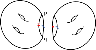
Figure 6.1. Double branched cover

Let $\mathcal{S}$ be a collection of conic points $p_{i}$ with cone angles $\leq\pi$. If $\#\mathcal{S}$ is even, we can pair conic points, for instance, $p,q$, in $\mathcal{S}$, and connect them with a smooth curve $\gamma_{p,q}$. If $p,q,r,s\in\mathcal{S}$, $(p,q)$ and $(r,s)$ are paired and $\gamma_{p,q}$ cross $\gamma_{r,s}$ at a regular point $a\in M$, let $U$ be a small open neighborhood of $a$that does not contain any conic points and any other crossings. To resolve the crossing at $a$, we remove the crossing $U\cap\left(\gamma_{p,q}\cup\gamma_{r,s}\right)$ and paste back $2$ smooth caps so that $(p,r)$ and $(q,s)$ are connected. We then resolve all crossings one by one. As a result, the points in $\mathcal{S}$ can be paired in a way such that the connecting curves $\gamma_{p,q}$ and $\gamma_{r,s}$ for any two pairs $(p,q)$ and $(r,s)$ do not cross each other. We take two copies of $M$ and obtain a double branched cover $\tilde{M}$ by first cutting along each connecting curve $\gamma_{p,q}$ and then gluing each side to another copy. $\tilde{M}$ will branch exactly at the points in $\mathcal{S}$.

If $\#\mathcal{S}$ is odd, we can add a regular point $q$ on $M$ to $\mathcal{S}$ which we viewed as a “singularity” with cone angle $2\pi$, we then make the branched double cover $\tilde{M}$ like before. The resulting space will have a singularity at $q$ with cone angle $4\pi$. The following lemma enables us to pick a regular point away from the curve shortening flow.

Lemma 6.4.

Suppose that $X(x,t)$ exists for $t\in[0,T)$. Then, there is a point $q\in M-\{p_{i}\}$ such that $\exists\epsilon,\delta>0$ for $t\in[T-\epsilon,T)$, $B_{\delta}(q)\cap\{X(x,t):\forall x\in S^{1}\}=\varnothing$.

Proof.

We argue by contradiction. Suppose that for any $q\in M-\{p_{i}\}$, there is a sequence of $\epsilon_{i}$ goes to 0 such that $t_{i}=T-\epsilon_{i}$ and $B_{\epsilon_{i}}(q)\cap X(\cdot,t_{i})\not=\varnothing.$ This, however, means that $\limsup_{t\to T}L(t)=\infty$, which is impossible. ∎

Suppose that the covering map is given by $\boldsymbol{\pi}:\tilde{M}\to M$. We can equip $\tilde{M}$ with the pull-back metric. We call $\tilde{O}\in\tilde{M}$ a doubled conic point if $\boldsymbol{\pi}(\tilde{O})=O\in\mathcal{S}$. Suppose that the cone angle at $O$ is $2(1+\beta)\pi$. Then, we can find a holomorphic coordinate $\xi$ near $O$, and a holomorphic coordinate $z$ near $\tilde{O}$ such that $\xi(O)=0,z(O)=0$, and

$$\boldsymbol{\pi}:z\mapsto z^{2}.$$

We see immediately that the pull-back metric is

$$\boldsymbol{\pi}^{*}g=|z^{2}|^{2\beta}e^{2h(z^{2})}|dz^{2}|^{2}=4|z|^{2(1+2\beta)}e^{2h(z^{2})}|dz|^{2}.$$

Thus, the cone angle at $\tilde{O}$ is $2(2+2\beta)\pi$. Let $U$ be a disk neighborhood of $O$. If $h(z)\in C^{2,\alpha}(U,O\beta)$, then $h(z^{2})\in C^{2,\alpha}(U,O(2\beta+1))$. Moreover, if $\beta\geq-\frac{1}{2}$, then $h(z^{2})\in C^{2,\alpha}(U)$ in the regular H$\mathbf{\ddot{o}}$lder space. In particular, if $\beta=-\frac{1}{2}$, then the pull-back metric $\boldsymbol{\pi}^{*}g$ is a $C^{2,\alpha}$ metric at $\tilde{O}$. To summarize, we can construct a double cover $\tilde{M}$ of $M$ branched over $\mathcal{S}$ or $\mathcal{S}\cup\{pt\}$ in the sense of the following Proposition.

Proposition 6.5.

Suppose that $(M,g,D)$ is a conic Riemann surface and $D=\sum_{i}\beta_{i}p_{i}.$ Let $k$ be the number of conic points of $M$. Let $\mathcal{S}$ be the collection of conic points $p_{i}$ with cone angles small than $\pi$. Then there is generalized Riemann surface $(\tilde{M},\tilde{g},\tilde{D})$ such that

1. There exists a branched double cover $\boldsymbol{\mathbf{\pi}}:\tilde{M}\to M$ which is locally isometric away from the branched points.

2. If $X(x,t)$ for $t\in[0,T)$ is a CSF on $M$, then the lifting $\tilde{X}$ on $\tilde{M}$ is also a CSF.

3. If $\#\mathcal{S}$ is even, then $\boldsymbol{\pi}$ is branched exactly at $\mathcal{S}$. $\tilde{M}$ is a conic Riemann surface with at most $2k-\#\mathcal{S}$ conic points and

   $$\tilde{D}=\sum_{p_{i}\in\mathcal{S}}(2\beta_{i}+1)p_{i}+\sum_{p_{i}\not\in\mathcal{S}}\beta_{i}\pi^{-1}(p_{i}).$$

4. If $\#\mathcal{S}$ is odd, then $\boldsymbol{\pi}$ is branched at $\mathcal{S}\cup\{\hat{p}\}$ for a regular point $\hat{p}$ of $M$. $\tilde{M}$ has at most $2k-\#\mathcal{S}+1$ singular points and

   $$\tilde{D}=\sum_{p_{i}\in\mathcal{S}}(2\beta_{i}+1)p_{i}+\hat{p}+\sum_{p_{i}\not\in\mathcal{S}}\beta_{i}\pi^{-1}(p_{i}).$$

   In this case, we can pick $\hat{p}$ away from a particular CSF on $M$ by Lemma 6.4.

7. CSF on conic surfaces

We study CSF on conic surfaces in this section. First, we rewrite Theorem 1.1 in the following form.

Theorem 7.1.

Let $(M,g)$ be a conic Riemann surface with divisor $D=\sum_{i=1}^{k}\beta_{i}p_{i}$. Suppose that $\mathcal{S}$ contains conic singularities with cone angles $\leq\pi$. Let $\Gamma_{t}$ be a curve shortening flow parametrized by $X(x,t)$. Suppose that $X(x,t)$ exists for $(x,t)\in S^{1}\times[0,T)$, $T<\infty$. Let $\mathbf{d}(\cdot,\cdot)$ be the distance function on $M$. Then, either $\mathbf{d}(\Gamma_{t},p)>c>0$ for all $t\in[0,T)$ and all $p\in\mathcal{S}$, or $\mathbf{d}(\Gamma_{t},p)\to 0$ uniformly for some $p\in\mathcal{S}$ as $t\to T$.

To prove this Theorem, we use comparison function $R(t)$ on the double branched cover $\tilde{M}$ described in Proposition 6.5. We will prove the boundedness of $R(t)$ with an additional assumption that the total length $L(t)$ remains positive.

Theorem 7.2.

Let $\tilde{M}$ be a double cover of $M$ branched at $\mathcal{S}$. Suppose that $X(x,t)$ exists for $t\in[0,T)$ and $L(t)>c>0$ for all $t\in[0,T)$. Let $\tilde{X}(x,t)$ be the lift of $X(x,t)$ on $\tilde{M}$. Let

$$R(t)=\sup_{x,y}e^{-Kt}\frac{\tilde{L}(t)}{\pi d_{\tilde{M}}(x,y,t)}\sin\frac{\pi\tilde{l}(x,y,t)}{\tilde{L}(t)},$$

where $\tilde{L}(t)=2L(t)$ is the total length of $\tilde{X}(\cdot,t)$, $\tilde{l}$ is the arc-length on $\tilde{X}(\cdot,t)$, and $d_{\tilde{M}}(x,y,t)$ is the distance on $\tilde{M}$ between $\tilde{X}(x,t)$ and $\tilde{X}(y,t)$. Then, there exists a constant $K=K(M,c)$ such that $R(t)$ is bounded by a universal constant depending on $R(0)$ and $M$.

Let us postpone the proof of Theorem 7.2 and give a quick proof of Theorem 7.1.

Proof of Theorem 7.1 assuming Theorem 7.2.

Let $\tilde{M}$ be the double cover of $M$ branched at $\mathcal{S}$. As $t\to T$, if ${\rm\mathbf{d}}_{M}(X(\cdot,t),p)\to 0$ for some $p\in\mathcal{S}$. Then, $\mathbf{d}_{\tilde{M}}(\tilde{X}(\cdot,t),\boldsymbol{\pi}^{-1}(p))\to 0$ as well. Here, $\mathbf{d}_{M}$ denote the distance function on $M$ and $\mathbf{d_{\tilde{M}}}$ denote the distance function on $\tilde{M}.$

If $\tilde{X}$ does not shrink to $p$, then $\lim_{t\to T}\tilde{L}(t)\geq c>0$. Let $\{(x_{i},t_{i})\}_{i=1}^{\infty}$ be a sequence such that $\tilde{X}(x_{i},t_{i})\to p$. Then, $\tilde{X}(x_{i}+\frac{\tilde{L}}{2},t_{i})\to p$ by the symmetry of the lifting. Now, evaluating at $(x_{i},t_{i})$ and $(x_{i}+\frac{\tilde{L}}{2},t_{i})$, we have

$$R(t_{i})\geq e^{-Kt_{i}}\frac{\tilde{L}(t_{i})}{\pi d_{\tilde{M}}(x_{i},x_{i}+\frac{\tilde{L}}{2},t_{i})}\sin\left(\frac{\pi}{2}\right)\geq e^{-KT}\frac{c}{\pi d_{\tilde{M}}(x_{i},x_{i}+\frac{\tilde{L}}{2},t_{i})},$$

where $d_{\tilde{M}}(x,y,t)=\mathbf{d}_{\tilde{M}}(X(x,t),X(y,t))$. The right hand side blows up as $i\to\infty$ because

$$d_{\tilde{M}}(x_{i},x_{i}+\frac{\tilde{L}}{2},t_{i})\leq 2\mathbf{d}_{\tilde{M}}(\tilde{X}(x_{i},t_{i}),\boldsymbol{\pi}^{-1}(p))\to 0.$$

However, $R(t)$ is bounded, so we have reached a contradiction. ∎

Now, we only need to prove the boundedness of $R(t)$. In order to apply the argument in Theorem 4.1, we have to take the derivatives of the distance function. For smooth surfaces, by choosing a big upper-bound for $R(t)$, we can always restrict ourselves inside a small disk in order to stay away from the cut locus. However, near conic singularities, cut locus can not be avoided.

Let $O$ be a conic point and let $A$ be a point in a disk neighborhood $U$ centered at $O$ such that ${\rm diam}(U)<\min\{r_{s},\pi/\sqrt{K_{M}}\}$ where $r_{s}$ is from Proposition 6.3. We denote the cut locus of $A$ as $\mathcal{C}_{A}$. By Rauch comparison principle, $\mathcal{C}_{A}\cap U$ does not contain conjugate points if ${\rm diam}(U)<\frac{\pi}{\sqrt{K_{M}}}$ . Therefore,

$$\mathcal{C}_{A}\cap U=\{B\in U:\exists{\rm geodesics}\ \gamma_{1}\not=\gamma_{2}\ {\rm realizing\ distance\ }\mathbf{d}(A,B)\}.$$

If $B\in\mathcal{C}_{A}\cap U$, there are $2$ shortest geodesics connecting $A$ and $B$. In fact, suppose that $3$ or more shortest geodesics connect $A$ and $B$. $2$ of the geodesics, denoted as $\gamma_{1},\gamma_{2}:[0,\mathbf{d}(A,B)]\to U$, will bound a simply-connected bigon $\Omega_{A,B}\subset U$ which contains no conic points. Since ${\rm diam}(\Omega_{A,B})<\frac{\pi}{\sqrt{K_{M}}},$ and the Gaussian curvature $\mathcal{K}<K_{M}$, we can apply Rauch comparison principle in $\Omega_{A,B}$ to show $\mathbf{d}(\gamma_{1}(t),\gamma_{2}(t))>0$. It contradicts to the fact that $\gamma_{i}(\mathbf{d}(A,B))=B$, $i=1,2$.

We will prove the following fact: If $Z_{N}(\cdot,\cdot,t)$ achieves local minimum at $(x,y)$ such that $X(x,t)$ is inside the cut locus of $X(y,t)$ near a conic point, then $Z_{N}$ can be replaced by some smooth functions which also achieve minimum at the same location.

Lemma 7.3.

Let $D_{r}(O)$ be a disk neighborhood of a conic point $O$. Suppose that $Z_{N}(\cdot,\cdot,t)$ achieves local minimum at $\bar{x},\bar{y}$ and $A=X(\bar{x},t)$, $B=X(\bar{y},t)$ are both in $D_{r}(O)\backslash\{O\}$. Then, $Z_{N}(\cdot,\cdot,t)$ is $C^{1}$ in a neighborhood of $(\bar{x},\bar{y})$. Moreover, if $B\in\mathcal{C}_{A}$ , then there exist two smooth functions $Z_{N}^{i}(\cdot,\cdot,t)$, $i=1,2$ such that $Z_{N}(x,y,t)=\min\{Z_{N}^{1}(x,y,t),Z_{N}^{2}(x,y,t)\}$ and $Z_{N}^{i}(\cdot,\cdot,t)$ both achieve local minimum at $(\bar{x},\bar{y})$.

Proof.

Let $f_{1}(y)$, $f_{2}(y)$ be two smooth functions, and $f(y):=\min\{f_{1}(y),f_{2}(y)\}$. Then, $f(y)$ is smooth away from the set $\mathcal{C}=\{y:f_{1}(y)=f_{2}(y)\}$. If $f(y)$ achieves a local minimum at $y_{0}\in\mathcal{C}$ then we claim that $y_{0}$ is a local minimum of both $f_{1}$ and $f_{2}$. Otherwise, we may assume that there exists a sequence $y_{i}\to y_{0}$, as $i\to\infty$ such that $f_{1}(y_{i})<f_{1}(y_{0})$. Then

$$f(y_{i})\leq f_{1}(y_{i})<f_{1}(y_{0})=f(y_{0}).$$

This contradicts to the fact that $f$ achieves a local minimum at $y_{0}$. So we have proved the claim. Moreover, we see that $f_{1}^{\prime}(y)=f_{2}^{\prime}(y)=0$.

We assume that $B\in\mathcal{C}_{A}$. Otherwise, the conclusion is obvious. Let $\mathbf{d}(\cdot,\cdot)$ be the distance function. Since $B\in\mathcal{C}_{A}$, there exist two geodesics $\gamma_{1},\gamma_{2}$ connecting $A,B$. We denote $d_{1}(A,B)={\rm Length}(\gamma_{1})$ and $d_{2}(A,B)={\rm Length}(\gamma_{2})$. We can extend each $\gamma_{i}$ to be a family of geodesics connecting $A$ and any point $Q$ near $B$. Thus, we can extend $d_{1}(A,Q)$ and $d_{2}(A,Q)$ smoothly for $Q$ in a neighborhood of $B$ such that

Figure 7.1. Distance function ($A,A^{\prime}$ are the same point)

$$\mathbf{d}(A,Q)=\min\{d_{1}(A,Q),d_{2}(A,Q)\}.$$

See Figure 7.1. For $y$ in a neighborhood of $\bar{y}$, we define

$$Z_{N}^{i}(\bar{x},y,t):=Nd_{i}(A,X(y,t))+\frac{L(t)}{\pi}\sin\left(\frac{\pi l(x,y,t)}{L(t)}\right)e^{-Kt}.$$

Then, each $Z_{N}^{i}(\bar{x},\cdot,t)$ is a function smoothly defined in a neighborhood of $\bar{y}$ and $Z_{N}(\bar{x},y,t)=\min\{Z_{N}^{1},Z_{N}^{2}\}$. Now, $B\in\mathcal{C}_{A}$ implies that $d_{1}(A,B)=d_{2}(A,B)$, and $Z_{N}^{1}(\bar{x},\bar{y},t)=Z_{N}^{2}(\bar{x},\bar{y},t)$. By the previous argument, we see that if $Z_{N}(\bar{x},\cdot,t)$ achieves local minimum at $\bar{y}$, then $Z_{N}^{i}(\bar{x},\cdot,t)$ also achieves local minimum at $\bar{y}$ and $\left(\frac{\partial Z_{N}}{\partial y}\right)(\bar{x},\bar{y},t)=0$ exists. By symmetry, $A\in\mathcal{C}_{B}$ and we can apply the same argument for $Z_{N}(\cdot,\bar{y},t)$. Thus, we have finished the proof. ∎

Proof of Theorem 7.2.

Lift $X(x,t)$ to be a CSF $\tilde{X}(x,t)$ on a double branched cover $\tilde{M}$ given in Proposition 6.5. Let $d_{0}=\min\{d_{M},\delta_{0}\}$, where $d_{M}$ is defined in Corollary 6.3 and $\delta_{0}$ is defined in Lemma 3.2. We pick $N>\max\{\frac{\tilde{L}(0)}{\pi d_{0}},R(0)\}$. If $Z_{N}(x,y,\bar{t})$ allows local variation at $\bar{x},\bar{y}$ , then the same argument in Theorem 4.1 can be applied. We require $L(t)>c>0$ to avoid subcase 2b and use (4.9), where the condition (4.10) on $K$ is replaced by $K>4C_{1}+\frac{4\pi^{2}}{c^{2}}$. If $X(\bar{x},\bar{t})$ is in the cut locus of $X(\bar{y},\bar{t})$, then we may assume that $X(\bar{x},\bar{t})$ and $X(\bar{y},\bar{t})$ is in a neighborhood of a conic singularity $O$ by the choice of $N$. Then, by Lemma 7.3,

$$Z_{N}(x,y,\bar{t})=\min\{Z_{N}^{1}(x,y,\bar{t}),Z_{N}^{2}(x,y,\bar{t})\},$$

for $(x,y)$ in a neighborhood of $(\bar{x},\bar{y})$, $Z_{N}^{1}(\bar{x},\bar{y},\bar{t})=Z_{N}^{2}(\bar{x},\bar{y},\bar{t})$, and both $Z_{N}^{i}(\cdot,\cdot,\bar{t})$ achieve local minimum at $(\bar{x},\bar{y}$). Then, we can apply the same arguments in Theorem 4.1 to either $Z_{N}^{1}(x,y,t)$ or $Z_{N}^{2}(x,y,t)$ which also yields contradictions. ∎

Appendix A Coordinates and geodesics on conic surfaces

In this appendix, we give the proof of the results in Proposition 6.3. We first prove the existence of an exponential map at each conic point. In [Tro90], Troyanov shows the existence of a geodesic polar coordinate near a conic point assuming a Gaussian curvature bound. Since we assume $h\in C^{\infty}(M-\{p_{i}\})\cap C^{2,\alpha}(M,D)$, the regularity of the polar coordinate is much easier to achieve.

Lemma A.1.

([Tro90]). Let $U$ be a neighborhood of conic point $p$ such that the divisor $D|_{U}=\beta p$, and the metric $g|_{U}$ is in the form of (6.1) for some $h\in C^{2,\alpha}(M,D)$. The following holds.

1. There is a $\rho_{0}>0$, an open neighborhood $V\subset U$ of $p$, and a map $\varphi:[0,\rho_{0})\times S^{1}\to V$ such that such that $\varphi(0,\theta)=p$, and $\varphi|_{(0,\rho_{0})\times S^{1}}\to V-\{p\}$ is smoothly diffeomorphic.

2. The pull-back metric

   (A.1) $$\varphi^{*}g=d\rho^{2}+\phi^{2}(\rho,\theta)d\theta^{2},$$

   where $\phi^{2}\in C^{2,\alpha}(D_{\rho_{0}}(p),\beta p)$, and $\lim_{\rho\to 0}\frac{\phi}{\rho}=1+\beta$.

We call $\varphi:[0,\rho_{0})\times S^{1}$ a geodesic polar coordinate near $p$.

Proof.

We provide a proof for readers’ convenience. Suppose that $g_{0}$ is a smooth background metric on $M$. Let $(r,\theta)$ be a geodesic polar coordinate on a geodesic disk $D_{r_{0}}^{g_{0}}(p)\subset(M,g_{0})$, such that $r(p)=0$, and $g_{0}=dr^{2}+\psi(r,\theta)^{2}d\theta^{2}$. Since $g_{0}$ is smooth, $\lim_{r\to 0}\psi/r=\lim_{r\to 0}\partial_{r}\psi=1.$ We may write $g=r^{2\beta}e^{2h(r,\theta)}(dr^{2}+\psi(r,\theta)^{2}d\theta^{2}).$ Let $\rho(r)=\int_{0}^{r}s^{\beta}e^{h(s,\theta)}ds$. We obtain a function $\rho$ in $D_{r_{0}}^{g_{0}}(p)$ strictly increasing in $r$and smooth in $(r,\theta)$ for $r>0$. We define

$$\varphi(\rho,\theta)=(r,\theta).$$

Note, $h$ is continuous and $\rho_{0}=\inf_{\partial D_{r_{0}}^{g_{0}}}\rho>0$. Let $V=\varphi([0,\rho_{0})\times S^{1})$. Then, $\varphi(0,\theta)=p$ and $\varphi$ is a smooth diffeomorphic map from $(0,\rho_{0})\times S^{1}$ to $V-\{p\}$. Notice that $\varphi^{*}g=d\rho^{2}+\phi(\rho,\theta)^{2}d\theta^{2},$ for $\phi(\rho,\theta)=r^{\beta}e^{h}\psi(r,\theta).$

$$\lim_{\rho\to 0}\phi/\rho =\lim_{\rho\to 0}\frac{\partial\phi}{\partial r}/\frac{\partial\rho}{\partial r}=\beta+\lim_{r\to 0}\left(\psi\frac{\partial h}{\partial r}+\frac{\partial\psi}{\partial r}\right)$$

$$=\beta+1.$$

Here $\lim_{r\to 0}\psi\frac{\partial h}{\partial r}=0$ since $h\in C^{2,\alpha}(M,D)$. Moreover, function $\psi(r,\theta)^{2}r^{2\beta}$ belongs to $C^{\infty}(U,\beta p)$. Hence,

$$\phi^{2}(\rho,\theta)=e^{2h}\psi^{2}r^{2\beta}\in C^{2,\alpha}(U,\beta p).$$

We have proved (1), (2). ∎

The next Lemma shows that the tangent cone at a conic point $p$ is uniquely determined and isometric to a flat cone. A tangent cone at $p$ is a pointed-Gromov-Hausdorff limiting space of $(M,\lambda_{i}^{-2}g,p)$ for a positive sequence $\lambda_{i}\to 0$. See [CC97]. Then, the exponential map at $p$ is well defined once we replace the tangent plane at $p$ by the tangent cone space at $p$.

Proposition A.2.

Assume the condition in Lemma A.1 and suppose that $\varphi:[0,\rho_{0})\times S^{1}\to V$ gives a polar coordinate near $p$. Let $T_{p}M$ be the tangent cone at the conic point $p$. The following statements hold.

1. The tangent cone $T_{p}M$ at $p$ is isometric to the flat cone $C_{(2+2\beta)\pi}$ with cone angle $(2+2\beta)\pi$.

2. The exponential map $\exp_{p}(v)$ from the tangent cone to $V$ is well-defined and diffeomorphic in a neighborhood of the cone tip..

Proof.

For a positive sequence $\lambda_{i}\to 0$, consider the pointed-Gromov-Hausdorff limiting space of $(M,\lambda_{i}^{-2}g,p)$. In the polar coordinate, for any $(\rho,\theta)\in(0,\infty)\times S^{1}$, let $\varphi_{i}(\rho,\theta):=\varphi(\lambda_{i}\rho,\theta)$. If $\lambda_{i}<\frac{\rho_{0}}{\rho}$,

$$\varphi_{i}(\rho,\theta)=\varphi(\lambda_{i}\rho,\theta)\in V-\{p\}.$$

Let $\phi_{i}(\rho)=\lambda_{i}^{-1}\phi(\lambda_{i}\rho).$ Then,

$$\lim_{i\to\infty}\phi_{i}(\rho)=\rho\lim_{i\to\infty}\frac{\phi(\lambda_{i}\rho,\theta)}{\lambda_{i}\rho}=(1+\beta)\rho,$$

by Lemma A.1 (2). Denote $\xi=\left((1+\beta)\rho\right)^{\frac{1}{1+\beta}}e^{\sqrt{-1}\theta}$.

(A.2) $$\lambda_{i}^{-2}\varphi_{i}^{*}g \to d\rho^{2}+(1+\beta)^{2}\rho^{2}d\theta^{2}$$

$$=|\xi|^{2\beta}|d\xi|^{2}.$$

Hence, the tangent cone $T_{p}M$ at $p$ is isometric to the flat cone $C_{\left(2+2\beta\right)\pi}$ defined by (1.2). The limit in (A.2) is independent of the sequence $\lambda_{i}$ which implies the uniqueness of the tangent cone. We have proved (1).

Let $v\in T_{p}M$. We may identify $v$ with $\left((1+\beta)\rho_{v}\right)^{\frac{1}{1+\beta}}e^{\sqrt{-1}\theta_{v}}$ in $\mathbb{C}$. By Lemma 1.4 in [Tro90], there is a neighborhood $U_{1}$ of $p$ such that for any $q\in U_{1}$, there is a unique geodesic $\gamma_{p,q}$ connecting $p$ and $q$. Moreover, if $q=\varphi(\rho_{1},\theta_{1})$, then $\gamma_{p,q}=\{\varphi(t\rho_{1},\theta_{1}):t\in[0,1]\}$, and the distance between $p,q$ is $\mathbf{d}(p,q)=\rho_{1}$. Thus, if $\rho_{v}$ is small, the exponential map $\exp_{p}(v):=\varphi(\rho_{v},\theta_{v})$ is well defined and corresponds to the shortest geodesic of length $\rho_{v}$ starting at $p$ in the direction of $v$. $\exp_{p}$ is a local diffeomorphism near the cone tip by Lemma A.1 (1). ∎

Remark A.3.

Let $\xi_{1},\xi_{2}\in T_{p}M$. Since $T_{p}M$ is isometric to $C_{\left(2+2\beta\right)\pi}$, we may identify $\xi_{1}=\left((1+\beta)\rho_{1}\right)^{\frac{1}{1+\beta}}e^{\sqrt{-1}\theta_{1}}$, and $\xi_{2}=\left((1+\beta)\rho_{2}\right)^{\frac{1}{1+\beta}}e^{\sqrt{-1}\theta_{2}}$, where $0\leq\theta_{1},\theta_{2}<2\pi$. The angle between $\xi_{1}$ and $\xi_{2}$ is $\delta\theta=(1+\beta)\min\{|\theta_{2}-\theta_{1}|,|2\pi+\theta_{1}-\theta_{2}|\}$. Then, the distance between $\xi_{1}$ and $\xi_{2}$ is given by

(A.3) $$\mathbf{d}_{T_{p}M}(\xi_{1},\xi_{2})^{2}=\rho_{1}^{2}+\rho_{2}^{2}-2\rho_{1}\rho_{2}\cos\left(\delta\theta\right).$$

Next, we show the existence of shortest geodesics for any pairs of points on $M$.

Proposition A.4.

Let $q_{1},q_{2}$ be $2$ points on $M$. There is a shortest smooth geodesic realizing the distance between $q_{1}$ and $q_{2}$.

Proof.

$(M,g,D)$ is a locally compact length space. It is also complete as a metric space. By Hopf-Rinow Theorem ([BBB⁺01], Section 2.5), the distance $l=\mathbf{d}(q_{1},q_{2})$ is realized by a piecewise geodesic $\gamma:[0,l]\to M$. The differentiable parts of $\gamma$ in the regular part of $M$ have to be smooth geodesics. If the interior of $\gamma$ does not contain any conic points, $\gamma$ is a smooth geodesic and we are done. If not, we argue by contradiction.

Let $p=\gamma(t_{1})$ be a conic point for some $t_{1}\in(0,l)$. Let $V$ be a neighborhood of $p$ in Lemma A.1 and $D|_{V}=\beta p$. Then, $\gamma\cap V$ contains at least $2$ geodesic segments connecting $p$. By Proposition A.2, we may assume that for some $0\leq\theta_{1},\theta_{2}<2\pi$,

$$\gamma(t)=\begin{cases}\varphi(t_{1}-t,\theta_{1}),&t\in[t_{0},t_{1}),\\ \varphi(t-t_{1},\theta_{2}),&t\in[t_{1},t_{2}).\end{cases}$$

Let $\tau=\min\{t_{1}-t_{0},t_{2}-t_{1}\}/2$, $\delta\theta=(1+\beta)\min\{|\theta_{2}-\theta_{1}|,|2\pi+\theta_{1}-\theta_{2}|\}$. Note $\delta\theta<\pi$, since $0<1+\beta<1$. Let $\{\lambda_{i}\}$ be a positive sequence which goes to $0$. By the minimizing property of $\gamma$,

(A.4) $$\mathbf{d}(\varphi(\lambda_{i}\tau,\theta_{1}),\varphi(\lambda_{i}\tau,\theta_{2}))=2\lambda_{i}\tau.$$

By (1) in Proposition A.2 and (A.3),

(A.5) $$\lim_{i\to\infty}\lambda_{i}^{-2}\mathbf{d}^{2}(\varphi(\lambda_{i}\tau,\theta_{1}),\varphi(\lambda_{i}\tau,\theta_{2})) =2\tau^{2}\left(1-\cos\delta\theta\right).$$

We can choose $0<\epsilon<\sqrt{\tau^{2}(1+\cos\delta\theta)}$. By (A.5), $\exists N>0$ such that if $i>N$,

$$|\mathbf{d}^{2}(\varphi(\lambda_{i}\tau,\theta_{1}),\varphi(\lambda_{i}\tau,\theta_{2}))-2\lambda_{i}^{2}\tau^{2}(1-\cos\delta\theta)|<\epsilon^{2}\lambda_{i}^{2}.$$

Then,

$$\mathbf{d}^{2}(\varphi(\lambda_{i}\tau,\theta_{1}),\varphi(\lambda_{i}\tau,\theta_{2}))<\lambda_{i}^{2}\tau^{2}\left(3-\cos\delta\theta\right)<4\lambda_{i}^{2}\tau^{2},$$

which contradicts to (A.4). We have proved the proposition. ∎

References

- [AB11] Ben Andrews and Paul Bryan. Curvature bound for curve shortening flow via distance comparison and a direct proof of grayson’s theorem. Journal für die reine und angewandte Mathematik (Crelles Journal), 2011(653):179–187, 2011.
- [AL86] Uwe Abresch and Joel Langer. The normalized curve shortening flow and homothetic solutions. Journal of Differential Geometry, 23(2):175–196, 1986.
- [Alt91] Steven J Altschuler. Singularities of the curve shrinking flow for space curves. 1991.
- [Ang91] Sigurd Angenent. On the formation of singularities in the curve shortening flow. Journal of Differential Geometry, 33(3):601–633, 1991.
- [BBB+01] Dmitri Burago, Iu D Burago, Yuri Burago, Sergei Ivanov, Sergei V Ivanov, and Sergei A Ivanov. A course in metric geometry, volume 33. American Mathematical Soc., 2001.
- [Bre14] Simon Brendle. Two-point functions and their applications in geometry. Bulletin of the American Mathematical Society, 51(4):581–596, 2014.
- [Car92] Manfredo Perdigao do Carmo. Riemannian geometry. Birkhäuser, 1992.
- [CC97] Jeff Cheeger and Tobias H Colding. On the structure of spaces with ricci curvature bounded below. i. Journal of Differential Geometry, 46(3):406–480, 1997.
- [CZ01] Kai-Seng Chou and Xi-Ping Zhu. The curve shortening problem. CRC Press, 2001.
- [Gag90] Michael E Gage. Curve shortening on surfaces. In Annales scientifiques de l’Ecole normale supérieure, volume 23, pages 229–256, 1990.
- [GH86] Michael Gage and Richard S Hamilton. The heat equation shrinking convex plane curves. Journal of Differential Geometry, 23(1):69–96, 1986.
- [Gra87] Matthew A Grayson. The heat equation shrinks embedded plane curves to round points. Journal of Differential geometry, 26(2):285–314, 1987.
- [Gra89] Matthew A Grayson. Shortening embedded curves. Annals of Mathematics, 129(1):71–111, 1989.
- [Ham93] Richard S Hamilton. Monotonicity formulas for parabolic flows on manifolds. Communications in Analysis and Geometry, 1(1):127–137, 1993.
- [Ham95] Richard S Hamilton. Harnack estimate for the mean curvature flow. Journal of Differential Geometry, 41(1):215–226, 1995.
- [Has16] Robert Haslhofer. Lectures on curve shortening flow. preprint, 2016.
- [Hui90] Gerhard Huisken. Asymptotic-behavior for singularities of the mean-curvature flow. Journal of Differential Geometry, 31(1):285–299, 1990.
- [Hui98] Gerhard Huisken. A distance comparison principle for evolving curves. Asian Journal of Mathematics, 2(1):127–133, 1998.
- [Oss78] Robert Osserman. The isoperimetric inequality. Bulletin of the American Mathematical Society, 84(6):1182–1238, 1978.
- [Tro90] Marc Troyanov. Coordonnées polaires sur les surfaces riemanniennes singulieres. In Annales de l’institut Fourier, volume 40, pages 913–937, 1990.
- [Yin10] Hao Yin. Ricci flow on surfaces with conical singularities. Journal of Geometric Analysis, 20(4):970–995, 2010.