Decomposition and embedding in the stochastic $GW$ self-energy

Abstract

We present two new developments for computing excited state energies within the $GW$ approximation. First, calculations of the Green’s function and the screened Coulomb interaction are decomposed into two parts: one is deterministic while the other relies on stochastic sampling. Second, this separation allows constructing a subspace self-energy, which contains dynamic correlation from only a particular (spatial or energetic) region of interest. The methodology is exemplified on large-scale simulations of nitrogen-vacancy states in a periodic hBN monolayer and hBN-graphene heterostructure. We demonstrate that the deterministic embedding of strongly localized states significantly reduces statistical errors, and the computational cost decreases by more than an order of magnitude. The computed subspace self-energy unveils how interfacial couplings affect electronic correlations and identifies contributions to excited-state lifetimes. While the embedding is necessary for the proper treatment of impurity states, the decomposition yields new physical insight into quantum phenomena in heterogeneous systems.

I Introduction

First-principles treatment of electron excitation energies is crucial for guiding the development of new materials with tailored optoelectronic properties. Localized quantum states became the focal point for condensed systems:Yu et al. (2017); Grosso et al. (2017); Yankowitz et al. (2018); Cao et al. (2018); Zondiner et al. (2020); Turiansky, Alkauskas, and Van de Walle (2020); Gottscholl et al. (2020) due to their long-range electronic correlation, the localized excitations exhibit tunability by interfacial phenomena.Wang et al. (2015); Qiu, da Jornada, and Louie (2017); Tartakovskii (2020); Yuan et al. (2020) Besides predicting experimental observables, theoretical investigations thus help to elucidate the interplay of the electron-electron interactions and the role of the environment.

The excited electrons and holes near the Fermi level are conveniently described by the quasiparticle (QP) picture: the charge carriers are characterized by renormalized interactions and a finite lifetime limited by energy dissipation, which governs the deexcitation mechanism. Quantitative predictions of QPs necessitate the inclusion of non-local many-body interactions.

The prevalent route to describe QPs in condensed systems employs the Green’s function formalism.Martin, Reining, and Ceperley (2016); Fetter and Walecka (2003) The excitation energy and its lifetime are inferred from the QP dynamics. The many-body effects are represented by the non-local and dynamical self-energy, $\Sigma$. In practice, $\Sigma$ is approximated by selected classes of interactions, forming a hierarchy of systematically improvable methods.Martin, Reining, and Ceperley (2016) The formalism also allows constructing the self-energy for distinct states with a different form of $\Sigma$.

Here we neglect the vibrational effects, and the induced density fluctuations dominate the response of the system to the excitation. The perturbation expansion is conveniently based on the screened Coulomb interaction, $W$, which explicitly incorporates the system’s polarizability. The neglect of the induced quantum fluctuations (while accounting for the induced density) leads to the popular $GW$ method.Hedin (1965); Hybertsen and Louie (1986); Aryasetiawan and Gunnarsson (1998); Martin, Reining, and Ceperley (2016) This approach predicts the QP gap, ionization potentials, and electron affinities in excellent agreement with experiments.Hedin (1965); Aryasetiawan and Gunnarsson (1998) Within the $GW$ approximation, $\Sigma$ is a product of $W$ and the Green’s function, $G$, in the time domain.

Conventional implementations of the $GW$ self-energy scale as $O(N^{4})$ with the system size, albeit with a small prefactor,Govoni and Galli (2015) and it is usually limited to few-electron systems. Stochastic treatment recasts the self-energy as a statistical estimator and employs sampling of electronic wavefunctions combined with the decomposition of operators.Neuhauser et al. (2014); Vlček et al. (2018); Vlcek et al. (2017) In practice, this formulation decreases the computational time significantly and leads to a linear scaling algorithm.Neuhauser et al. (2014); Vlcek et al. (2017); Vlček et al. (2018)

The stochastic approach uses real-space random vectors that sample the Hilbert space of the electronic Hamiltonian. The statistical error in $\Sigma$ is governed by the number of vectors, which are used for the decomposition of $G$ and the evaluation of $W$. While extended systems with delocalized states are treated efficiently, the statistical fluctuations are more significant for localized orbitals.Brooks et al. (2020) This translates to an increased computational cost for defects, impurities, and molecules.Brooks et al. (2020); Vlcek et al. (2017) Further, too high fluctuations potentially hinder proper convergence and may result in sampling bias.

Here we overcome this difficulty by constructing a hybrid deterministic-stochastic approach. We show how to efficiently decompose $G$ and $W$ in real-time and embed the strongly localized states. In this formalism, the problematic orbitals are treated explicitly without relying on their sampling by random vectors. A similar embedding scheme was so far employed only in static ground-state calculations.Li et al. (2019) The decomposition is general and can be used to sample arbitrary excitations. Naturally, it is especially well suited for spatially or energetically isolated electronic states. Further, we employ the decomposition technique to compute $\Sigma$ stochastically from an arbitrarily large subspace of interest. We show the self-energy separation disentangles correlation contributions from different spatial regions of the system.

After deriving the formalism of the self-energy embedding and decomposition, we illustrate our methods numerically for nitrogen vacancy in large periodic cells of hBN. This system represents a realistic simulation of a prototypical single-photon emitter.Tran et al. (2016); Grosso et al. (2017); Exarhos et al. (2017); Li et al. (2019); Mendelson et al. (2019) First, we demonstrate the reduction of the stochastic error for the defect states in the hBN monolayer. Next, we study the interaction of the defect in the hBN-graphene heterostructure.

II Computing quasiparticle energies

II.1 Self-energy and common approximations

The Green’s function ($G$), a time-ordered correlator of creation and annihilation field operators, describes the dynamics of an individual quasiparticle. The poles of $G$ fully determine the single-particle excitations (as well as many other properties).

Solving directly for G is often technically challenging (or outright impossible). Alternatively, the Green’s function is often sought via a perturbative expansion of the electron-electron interactions on top of a propagator of non-interacting particles (i.e., the non-interacting Green’s function, $G_{0}$). The two quantities are related via the Dyson equation $G^{-1}=G_{0}^{-1}-\Sigma$, where $\Sigma$ is a self-energy accounting, in principle, for all the many-body effects absent in $G_{0}$.

Calculations usually employ only a truncated expansion of the self-energy. Despite ongoing developments,Maggio and Kresse (2017); Hellgren, Colonna, and de Gironcoli (2018); Vlcek (2019) the most common approach is limited to the popular $GW$ approximation to the self-energy, which is composed of the non-local exchange ($\Sigma_{X}$) and polarization ($\Sigma_{P}$) terms. In the time-domain, the latter operator is expressed as:

$$\Sigma_{P}({\bf r},{\bf r}^{\prime},t)=iG({\bf r},{\bf r}^{\prime},t)W_{P}({\bf r},{\bf r}^{\prime},t^{+}),$$ (1)

where $W_{P}$ is the time-ordered polarization potential due to the time-dependent induced charge density Vlček et al. (2018). The potential is conveniently expressed using the reducible polarizability $\chi$ as

$$\begin{split}W_{P}({\bf r},&{\bf r}^{\prime},t)=\\ &\int\int\nu({\bf r},{\bf r}^{\prime\prime})\chi({\bf r}^{\prime\prime}{\bf r}^{\prime\prime\prime},t)\nu({\bf r}^{\prime\prime\prime},{\bf r}^{\prime})d{\bf r}^{\prime\prime}d{\bf r}^{\prime\prime\prime}\end{split}$$ (2)

Evaluating the action of $W_{P}$ on individual states is the practical bottleneck of the $GW$ approach. Hence, despite Eq. 1 requires a self-consistent solution, it is commonly computed only as a “one-shot” correction. In practice, Eq. 1 thus contains only $G_{0}$ and $W_{0}$. Both quantities are constructed from the mean-field Hamiltonian, $H_{0}$, comprising one-body terms and local Hartree, ionic, and exchange-correlation potentials. For $W_{P}$, it is common to employ the random phase approximation (RPA). Beyond RPA approaches are more expensive and, in general, do not improve the QP energies unless higher-order (vertex) terms are included in $\Sigma$.Lewis and Berkelbach (2019); Vlcek (2019)

Within this one-shot framework, the QP energies becomeMartin, Reining, and Ceperley (2016)

$$\varepsilon^{QP}=\varepsilon^{0}+\langle\phi|\Sigma_{X}+\Sigma_{P}(\omega=\varepsilon^{QP})-v_{xc}|\phi\rangle,$$ (3)

where $\varepsilon^{0}$ are eigenvalues of $H_{0}$ and $v_{xc}$ is the (approximate) exchange-correlation potential. In Eq. 3, $\Sigma_{P}$ is in the frequency domain.

II.2 The stochastic approach to the self-energy

The stochastic $G_{0}W_{0}$ method seeks the QP energy via random sampling of wavefunctions and decomposition of operators in the real-time domain.Neuhauser et al. (2014); Vlcek et al. (2017); Vlček et al. (2018) The expectation value of $\Sigma$ is expressed as a statistical estimator. The result is subject to fluctuations that decrease with the number of samples as $1/\sqrt{N}$.

In this formalism, the polarization self-energy expression is separable.Neuhauser et al. (2014); Vlcek et al. (2017); Vlček et al. (2018) Specifically, for a particular $H_{0}$ eigenstate $\phi$, the perturbative correction becomes:

$$\langle\phi|\Sigma_{P}(t)|\phi\rangle =\langle\phi|iG_{0}(t)W_{P}(t)|\phi\rangle$$

$$\simeq\frac{1}{N_{\bar{\zeta}}}\sum_{\bar{\zeta}}\int\phi({\bf r})\zeta({\bf r},t)u_{\zeta}({\bf r},t)d^{3}{\bf r},$$ (4)

where $u_{\zeta}(r,t)$ is an induced charge density potential, and $\zeta$ is a random vector used for sampling of $G_{0}$ (discussed in detail in the next section). The state $\zeta$ at time $t$ is

$$|\zeta(t)\rangle~{}\equiv~{}U_{0,t}P_{\mu}|{\zeta}\rangle,$$ (5)

where the $U_{0,t}$ is time evolution operator

$$U_{0,t}\equiv e^{-iH_{0}t}.$$ (6)

The projector $P_{\mu}$ selects the states above or below the chemical potential, $\mu$, depending on the sign of $t$. In practice, $P_{\mu}$ is directly related to the Fermi-Dirac operator.Baer and Neuhauser (2004); Gao et al. (2015); Neuhauser et al. (2016); Vlček et al. (2018) Since the Green’s function is a time-ordered quantity, the vectors in the occupied and unoccupied subspace are propagated backward or forward in time and contribute selectively to the hole and particle non-interacting Green’s functions.

The induced potential $u({\bf r},t)$ represents the time-ordered potential of the response to the charge addition or removal:

$$u({\bf r},t)=\int W_{P}({\bf r},{\bf r}^{\prime},t)\bar{\zeta}({\bf r}^{\prime})\phi({\bf r}^{\prime})d^{3}{\bf r}^{\prime},$$ (7)

where $\bar{\zeta}$ spans the entire Hilbert space.Neuhauser et al. (2014); Vlcek et al. (2017); Vlček et al. (2018)

In practice, we compute $u$ from the retarded response potential, which is $\tilde{u}=\int\tilde{W}_{P}({\bf r},{\bf r}^{\prime},t)\bar{\zeta}({\bf r}^{\prime})\phi({\bf r}^{\prime})d^{3}{\bf r}^{\prime}$; the time-ordering step affects only the imaginary components of the Fourier transforms of $u$ and $\tilde{u}$.Fetter and Walecka (2003); Vlcek et al. (2017); Vlček et al. (2018)

The retarded response, $\tilde{u}$, is directly related to the time-evolved charge density $\delta n(\vec{r},t)\equiv n({\bf r},t)-n(\vec{r},t=0)$ induced by a perturbing potential $\delta v$:

$$\tilde{u}({\bf r},t)=$$

$$\int\int\int\nu({\bf r},{\bf r}^{\prime\prime}) \chi({\bf r}^{\prime\prime},{\bf r}^{\prime\prime\prime},t)\delta v({\bf r}^{\prime\prime\prime},{\bf r}^{\prime})d{\bf r}^{\prime}d{\bf r}^{\prime\prime}d{\bf r}^{\prime\prime\prime}$$

$$\equiv\int\nu({\bf r},{\bf r}^{\prime})\delta n({\bf r}^{\prime},t){{\rm d}}{\bf r}^{\prime}$$ (8)

where we define a perturbing potential

$$\delta v=\nu({\bf r},{\bf r}^{\prime}){\bar{\zeta}}({\bf r}^{\prime})\phi({\bf r}^{\prime}).$$ (9)

Note that $\delta v$ is explicitly dependent on the state $\phi$ and the $\bar{\zeta}$ vector; the latter is part of the stochastically decomposed $G_{0}$ operator.

The stochastic formalism further reduces the cost of evaluating $\tilde{u}$. Instead of computing $\delta n(\vec{r},t)$ by a sum over single-particle states, we use another set of random vectors $\left\{\eta\right\}$ confined to the occupied subspace. Time-dependent density $n({\bf r},t)$ thus becomesNeuhauser et al. (2014); Vlcek et al. (2017); Vlček et al. (2018); Gao et al. (2015); Rabani, Baer, and Neuhauser (2015); Neuhauser et al. (2016)

$$n({\bf r},t)=\lim_{N_{\eta}\to\infty}\frac{1}{N_{\eta}}\sum_{l}^{N_{\eta}}|\eta_{l}({\bf r},t)|^{2},$$ (10)

where $\eta_{l}$ is propagated in time using $U_{0,t}$, and $H_{0}$ in Eq. 6 is implicitly time-dependent. As common,Hybertsen and Louie (1986); Martin, Reining, and Ceperley (2016) we resort to the density functional theory (DFT) starting point. Since $H_{0}$ is therefore a functional of $n(\vec{r},t)$, the same holds for the time evolution operator:

$$\left|\eta(t)\right\rangle=U_{0,t}[n(t)]\left|\eta\right\rangle.$$ (11)

Further, we employ RPA when computing $\tilde{u}$; this corresponds evolution within the time-dependent Hartree approximation.Baroni, de Gironcoli, and Dal Corso (2001); Baer and Neuhauser (2004); Neuhauser and Baer (2005)

Practical calculations use only a limited number of random states. Consequently, the time evolved density exhibits random fluctuations at each space-time point. To resolve the response to $\delta v$, we use a two-step propagation whose difference is the $\delta n$ that typically converges fast with $N_{\eta}$.Neuhauser et al. (2014); Vlcek et al. (2017); Vlček et al. (2018)

III Embedded Deterministic Subspace

The stochastic vectors $\left\{\zeta\right\}$ and $\left\{\eta\right\}$, introduced in the preceding section, are constructed on a real-space grid and sample the occupied (or unoccupied) states. The number of these vectors ($N_{\zeta}$ and $N_{\eta}$) is increased so that the statistical errors are below a predefined threshold. Further, the underlying assumption is that $\left\{\zeta\right\}$ and $\left\{\eta\right\}$ sample the Hilbert space uniformly.

Here, we present a stochastic approach restricted only to a subset of states, while selected orbitals, $\left\{\phi\right\}$, are treated explicitly and constitute an embedded subspace. We denote this set as the $\{\phi\}$-subspace. In the context of the $G_{0}W_{0}$ approximation, we use the hybrid approach for (i) the Green’s function, (ii) the induced potential, or (iii) both $G_{0}$ and $u$ simultaneously. In the following, we present each case separately.

First,

the non-interacting Green’s function is decomposed into two parts (omitting for brevity the space-time coordinates):

$$G_{0}\equiv\tilde{G}_{0}+G^{\phi}_{0},$$ (12)

where $G^{\phi}_{0}$ is the Green’s function of the constructed explicitly from $\left\{\phi\right\}$ as

$$G^{\phi}_{0}({\bf r},{\bf r}^{\prime},t)=\sum_{j\in\{\phi\}}(-1)^{\theta(t)}\,i\phi_{j}({\bf r})\phi^{*}_{j}({\bf r}^{\prime})e^{-i\varepsilon_{j}t}$$ (13)

where $\theta$ is the Heaviside step function responsible for the time-ordering (corresponding to particle and hole contributions to $G_{0}$). The complementary part, $\tilde{G}_{0}$, is sampled with random states as in Eq. 4.

Unlike in the fully stochastic approach (where no $G^{\phi}_{0}$ term is present), the sampling vectors are constructed as orthogonal to the $\{\phi\}$-subspace, i.e.:

$$\left|\bar{\zeta}\right\rangle=\left(1-P_{\phi}\right)\left|\bar{\zeta}_{0}\right\rangle.$$ (14)

Here, $\bar{\zeta}_{0}$ spans in principle, the entire Hilbert space, and $P_{\phi}$ is:

$$P_{\phi}=\sum_{j\in\left\{\phi\right\}}\left|\phi_{j}\middle\rangle\middle\langle\phi_{j}\right|.$$ (15)

The construction of $\tilde{G}_{0}$ remains the same as in the fully stochastic case: $\tilde{G}_{0}$ is decomposed by a pair of vectors $\bar{\zeta}$ and $\zeta(t)$, cf. Eqs. (14), (5) and (6).

Note that it is possible to generalize the projector $P_{\phi}$, Eq.(15), to an arbitrary $\left\{\phi\right\}$-subspace. The particular choice of $\phi$ does not affect the decomposition of the Green’s function, Eq. (12), or the time evolution of $\zeta(t)$. However, the dynamics of $G_{0}^{\phi}$ would require explicit action of $U_{0,t}$ on $\phi$ that is, in principle, not an eigenstate of $H_{0}$. We do not pursue this route here and select $\{\phi\}$-subspace composed from the starting point eigenstates.

Second,

the retarded induced potential $\tilde{u}$ is decomposed through partitioning of the time-dependent charge density, cf., Eq. (II.2), (omitting the space-time coordinates):

$$n\equiv\tilde{n}+n_{\phi},$$ (16)

where the $n_{\phi}$ is the density constructed from occupied states $\phi$ (which we assume to be mutually orthogonal):

$$n_{\phi}({\bf r},t)=\sum_{j\in\{\phi\}}f_{j}\left|\phi_{j}({\bf r},t)\right|^{2}.$$ (17)

Here, $f_{j}$ is the occupation of the $j^{\rm th}$ state. Note that choosing $\phi$ within the unoccupied subspace is meaningless in this context. The complementary part, $\tilde{n}$, is given by stochastic sampling, Eq. (10), that employs random vectors $\tilde{\eta}$:

$$\left|\widetilde{\eta}\right\rangle=\left(1-\tilde{P}_{\phi}\right)\left|\eta\right\rangle,$$ (18)

where $\eta$ spans the entire occupied subspace and

$$\tilde{P}_{\phi}=\sum_{j\in\left\{\phi\right\}}f_{j}\left|\phi_{j}\middle\rangle\middle\langle\phi_{j}\right|.$$ (19)

The time propagation of the charge density is similar to the fully stochastic case. The deterministic and stochastic vectors evolve as:

$$\left|\phi_{j}(t)\right\rangle =U_{0,t}[n_{\phi}(t),\tilde{n}(t)]\left|\phi_{j}\right\rangle$$ (20)

$$\left|\tilde{\eta}(t)\right\rangle =U_{0,t}[n_{\phi}(t),\tilde{n}(t)]\left|\tilde{\eta}\right\rangle,$$ (21)

where $U_{0,t}$ is explicitly expressed as a functional of the two density contributions from Eq. (16). Note that these expressions are analogous to Eq. (11).

Third,

both partitionings are used in conjunction. While $G_{0}$ contains contributions from both occupied and unoccupied states, only the former are included in $\tilde{u}$. The combined partitioning may use entirely different subspaces for the Green’s function and the induced potential. In Section V.3, we employ the decomposition in both terms because it yields the best results and significantly reduces statistical fluctuations.

IV Decomposition of the stochastic polarization self-energy

In the preceding section, we partition retarded induced potential and the Green’s function, intending to decrease stochastic fluctuations in the self-energy. Here, we use the partitioning to achieve the second goal of this paper – to determine the contribution to $\Sigma_{P}(\omega)$.

Conceptually, we want to address quasiparticle scattering by correlations from a particular subspace. In the expression for $\Sigma_{P}(\omega)$, Eq. (4), this corresponds to accounting for selected charge density fluctuations in $\tilde{u}$. In practice, we construct the subspace polarization self-energy as:

$$\langle\phi|\Sigma^{s}_{P}(t)|\phi\rangle=\frac{1}{N_{\bar{\zeta}}}\sum_{\bar{\zeta}}\int\phi({\bf r})\zeta({\bf r},t)u^{s}_{\zeta}({\bf r},t)d^{3}{\bf r},$$ (22)

where we introduced the subspace induced potential $u^{s}_{\zeta}$ which is obtained from its retarded form (in analogy to Eq. (II.2)):

$$\tilde{u}^{s}_{\zeta}({\bf r},t)=\int\nu({\bf r},{\bf r}^{\prime})\delta n^{s}({\bf r}^{\prime},t){{\rm d}}{\bf r}^{\prime}.$$ (23)

This potential stems from the induced charge density that includes contributions only from selected orbitals $\{\phi\}$. Note that $n^{s}({\bf r}^{\prime},t)$ is obtained either from individual single-particle states or from the stochastic sampling of the $\{\phi\}$-subspace under consideration.

If the set of $\phi$ states is large, it is natural to employ the stochastic approach; the density is sampled according to Eq. (10) with vectors $\eta^{s}$ prepared as:

$$\left|\eta^{s}\right\rangle=\tilde{P}_{\phi}\left|\eta\right\rangle$$ (24)

where the projector is in Eq. (19) and vectors $\eta$ span the entire occupied subspace.

The time evolution of $\eta^{s}$ follows Eq. (11), i.e., it is governed by the operator $U_{0,t}$ that depends on the total time-dependent density:

$$\left|\eta^{s}(t)\right\rangle=U_{0,t}[n(t)]\left|\eta^{s}\right\rangle.$$ (25)

Hence, despite $\Sigma_{P}^{s}(t)$ contains only fluctuations from a particular subspace, the calculation requires knowledge of the time evolution of both $n^{s}$ and $n$.

In practice, we employ a set of two independent stochastic samplings: (i) vectors $\left|\eta\right\rangle$ describing the entire occupied space, and (ii) vectors $\left|\eta^{s}\right\rangle$ confined only to the chosen $\{\phi\}$-subspace. The first set characterizes the total change density fluctuation and enters $U_{0,t}$ in Eq. 25.

V Numerical results and discussion

V.1 Computational details

In this section, we will demonstrate the capabilities of the method introduced above. The starting-point calculations are performed with a real-space DFT implementation, employing regular grids, Troullier-Martins pseudopotentials,Troullier and Martins (1991) and the PBEPerdew and Wang (1992) functional for exchange and correlation. We investigate finite and 2D infinite systems using modified periodic boundary conditions with Coulomb interaction cutoffs.Rozzi et al. (2006)

The numerical verification for the SiH₄ molecule is in section V.2. To converge the occupied $H_{0}$ eigenvalues to $<5$ meV, we use a kinetic energy cutoff of 26 $E_{h}$ and $64\times 64\times 64$ real-space grid with the step of 0.3 $a_{0}$.

Large calculations for the $V_{N}$ defect in hBN monolayer and in hBN heterostructure with graphene are in sections V.3 and V.4. In both cases, we consider relaxed rectangular 12$\times$6 supercells containing 287 and 575 atoms. We performed a structural optimization in QuantumEspresso codeGiannozzi et al. (2017) together with Tkatchenko-Scheffler’s total energy corrections.Tkatchenko and Scheffler (2009) The heterostructure is built with an interlayer distance of 3.35 Å.

The $GW$ calculations were performed using a development version of the StochasticGW code.Neuhauser et al. (2014); Vlček et al. (2018); Vlcek et al. (2017) The calculations employ an additional set of 20,000 random vectors used in the sparse stochastic compression used for time-ordering of $\tilde{u}$Vlček et al. (2018). The time propagation of the induced charge density is performed for maximum propagation time of 50 a.u., with the time-step of 0.05 a.u.

V.2 Verification using molecular states

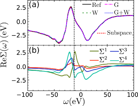
Figure 1: Verification for the SiH₄ molecule. (a) The comparison of the total self-energies of the highest occupied state (HOMO) obtained with reference and embedding schemes. The figure demonstrates that all five approaches yield identical $\Sigma(\omega)$. In the plot, G denotes the decomposition scheme where HOMO is embedded in the Green’s function; W denotes the calculation with HOMO state embedded in screened Coulomb potential; G+W corresponds to simultaneous decomposition of G and W. The red-dashed line represents the sum over subspace contributions shown in the panel below. (b) Subspace self-energy of the HOMO state that contains only a contribution of a specific state $i$, denoted as $\Sigma^{i}$ in the figure’s legend.

We verify the implementation of the methods presented in Sections III and IV on SiH₄ molecule. In particular, we test separately : (i) the construction of the embedding schemes, (ii) decomposition of the time propagation, and (iii) the evaluation of the subspace self-energy.

The reference calculation employs only one level of stochastic sampling (for the Green’s function, while the rest of the calculation is deterministic). For small systems, this approach converges fast as the stochastic fluctuations are small.Vlček et al. (2018); Vlcek et al. (2017) Yet, we need $N_{\zeta}=1,500$ vectors to decrease the QP energies errors below 0.08 eV. An illustration of the self-energy for the HOMO state of SiH₄ is in Fig. 1; everywhere in the figure, the stochastic error is below $0.13$ eV for all frequencies.

We first inspect the results for an embedded deterministic subspace. Fig. 1 shows that the different schemes for the explicit treatment of the HOMO state, Section III, produce the same self-energy curve. The inclusion of HOMO in $W$ is combined with the stochastic sampling of the three remaining orbitals by $N_{\eta}=$16 random vectors. Note that it is not economical to sample the action of $W_{P}$ for small systems,Vlcek et al. (2017); Vlček et al. (2018) and this calculation serves only as a test case. This treatment yields a statistical error of 0.08 eV, i.e., the same as the reference calculation despite the additional fluctuations due to the $\eta$ vectors.

When the HOMO orbital is explicitly included in $G$, the resulting statistical error is below the error of the reference calculation (0.05 eV). Such a result is expected since the reference relies on the stochastic sampling of the Green’s function. The same happens when the frontier orbital is in both $G$ and $W$ ($N_{\eta}=$16 random vectors sample the induced charge density). Tests for other states are not presented here but lead to identical conclusions.

Next, we verify that the density entering the time-evolution operator $U_{0,t}[n(t)]$ can be constructed from different states than it is acting on. Namely, the induced charge and the time-dependent densities may be sampled and built by different means. To demonstrate this, we propagate each of the $H_{0}$ eigenstates with $U_{0,t}[n(t)]$, where $n(t)$ is stochastically sampled by $N_{\eta}$=16 random vectors. Only the induced charge density, entering Eq. (II.2), is computed from the $\{\phi\}$ eigenvectors. The agreement with the reference self-energy curve is excellent with differences smaller than the standard deviations at each frequency point; see Fig. 1a.

Finally, we inspect the subspace self-energy in which $U_{0,t}[n(t)]$ employs the total charge density sampled by $N_{\eta}$=16 random vectors. In Fig. 1b shows four different $\Sigma^{s}(\omega)$ curves corresponding to the contributions of individual $H_{0}$ eigenstates. Since the eigenstates are orthogonal, the total self-energy is simply the sum of individual $\Sigma^{s}(\omega)$ components. The additivity of the subspace self-energies is demonstrated numerically in Fig. 1a. The subspace results illustrate that HOMO and the bottom valence orbital exhibit the largest amplitudes of $\Sigma_{P}^{s}$; hence, these two states dominate the correlation near the ionization edge.

V.3 Deterministic treatment of localized states

The deterministic subspace embedding should numerically stabilize the stochastic sampling and decreases the computational cost. To test the methodology on a realistic system, we consider the electronic structure of an infinitely periodic hBN monolayer containing a single nitrogen vacancy ($V_{N}$) per a unit cell with dimensions of $3.0\times 2.6$ nm. The system comprises 1147 electrons with the defect state being singly occupied and hence positioned at the Fermi level.

In the current calculations, we enforce spin degeneracy. The reason is twofold: (i) half populated states are strongly polarizable, and they exhibit stronger stochastic fluctuations in the time evolution. They are thus a more stringent test of the embedding. (ii) In Section V.4, we compare the monolayer with a heterostructure to determine the role of substrate material on the self-energy. In the heterostructure, the magnetic splitting of spin-up/down components disappears.Park, Park, and Kim (2014)

The relaxed monolayer geometry shows only mild restructuring. The vacancy introduces three localized states with $C_{3}$ and $C_{2}$ spatial symmetry. The former ($C_{3}$) is singly occupied and forms an in-gap state. The latter state is doubly degenerate and pushed high in the conduction region. Due to the enforced spin-degeneracy, the electron-electron interactions are increased and $C_{2}$ appears higher than in the previous calculationsAttaccalite et al. (2011); Huang and Lee (2012); Tran et al. (2016); McDougall et al. (2017). The $C_{3}$ and $C_{2}$ single-particle wavefunctions are illustrated in Fig. 2.

We first focus on the delocalized top valence and bottom conduction states. The fully stochastic calculations converge fast for both of them. The charge density fluctuations are sampled by $N_{\eta}=8$ vectors, and the Green’s function requires $N_{{\zeta}}$=1500 to yield QP energies with statistical errors below 0.03 eV for the valence band maximum (VBM). The error for the conduction band minimum (CBM) is $<0.01$ eV. The computed resulting quasiparticle band-gap is $6.49\pm 0.04$ eV, in excellent agreement with previous calculations and experiments (providing a range of values between 6.1 and 6.6 eV).Levinshtein, Rumyantsev, and Shur (2001); Fuchs et al. (2007); Hüser, Olsen, and Thygesen (2013)

To investigate the electronic structure in greater detail, we employ the projector-based energy-momentum analysis based on supercell band unfolding.Popescu and Zunger (2012); Huang et al. (2014); Medeiros, Stafström, and Björk (2014); Brooks et al. (2020) In practice, the individual wavefunctions within our simulation cell are projected onto the Brillouin zone of a single hBN unit cell. The resulting bandstructure is shown in Fig. 2a. Since our calculations employ a rectangular supercells, the critical point K of the hexagonal Brillouin zone appears between the $\Gamma$ and X points (marked on the horizontal axis by $\star$). The figure shows that the fundamental band gap is indirect; the direct transition is $7.39\pm 0.04$ eV in extremely close to the results for the pure hBN monolayer (reported to be in a range between 7.26 and 7.37 eV ).Hüser, Olsen, and Thygesen (2013); Cudazzo et al. (2016); Paleari et al. (2018)

The defect states appear as flat bands, labeled in Fig. 2 by their symmetry. As expected from the outset, the stochastic calculations for $C_{3}$ exhibit large fluctuations. While each sample is numerically stable, random vectors produce a self-energy curve with a significant statistical error at each frequency point, i.e., the time evolution is strongly dependent on the initial choice of $\{\zeta\}$ and $\{\eta\}$. In this example, only the $C_{3}$ state exhibits such behavior.

In Fig. 2 illustrates the self-energies for the band edge and the defect states. For all the cases, the plots show the spread of the $\Sigma_{P}(\omega)$ curves: these correspond to the outer envelope for 15 distinct calculations, each employing 100 $\zeta$ sampling vectors (combined with $N_{\eta}=8$ each). For the $C_{3}$ defect state, the stochastic sampling is possibly biased. The variation is three times as big as the spread of the VBM, and almost seven times larger compared to CBM. Away from the QP energy, the fluctuations increase even further; the spread of the samples becomes two times larger near the maximum of $\Sigma_{P}$ at $-20$ eV. The convergence of the QP energy is poor, and the low sample standard deviation (roughly twice as big as for VBM) suggests incorrect statistics. In practice, each sampling yields a self-energy curve that lies outside of the standard deviation of the previous simulation.

The deterministic embedding remedies insufficient sampling without increasing the computational cost. Naturally, we select the $C_{3}$ defect state and treat it explicitly (while randomly sampling the rest of the orbitals). Hence, according to the notation of Section III, the $\{\phi\}$-subspace contains only a single orbital.

The decomposition of the non-interacting Green’s function follows Eq. (12) and stabilizes the sampling. The spread of the self-energy curves decreases approximately three times for a wide range of frequencies. With the embedded $C_{3}$ state, the statistical error of the QP energy decreases smoothly and uniformly with the number of samples. Each new sampling falls within the error of the calculations. Yet, the final statistical error (0.03 eV) is less than 10% larger than for the delocalized states.

The decomposition of the induced charge density alone is less promising. Fundamentally, $\delta n({\bf r},t)$ contains contributions from the entire system, and a small $\{\phi\}$-subspace will unlikely lead to drastic improvement. Indeed, the statistical errors and convergence behavior remain the same as for the fully stochastic treatment.

Embedding of the localized state in both $G_{0}$ and $\delta n({\bf r},t)$ is, however, the best strategy. If both decompositions use the same (or overlapping) $\{\phi\}$-subspace, the induced charge density and the potential $\delta v$, Eq. (9), share (at least some) $\phi$ states. Consequently, the sampling of $\Sigma_{P}(\omega)$ becomes less dependent on the particular choice of $\zeta$ vectors, which sample only states orthogonal to $\{\phi\}$. Indeed, the embedding of a single localized state in $G$ and $W$ results in a nearly four-fold reduction of the statistical fluctuation that translates to more than an order of magnitude savings in the computational time. The error of the QP energy of the $C_{3}$ state is approximately half of the error for VBM (16 meV for $N_{\zeta}=1,500$).

For completeness, we also applied the three types of embedding on VBM, which does not suffer from bias or large statistical errors. Unlike for the localized state, we observe only a negligible reduction of the fluctuations. For delocalized states, the fully stochastic sampling is thus sufficient as expected from our previous work.Brooks et al. (2020); Vlček et al. (2018); Vlcek et al. (2017)

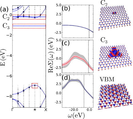
Figure 2: Deterministic embedding for the nitrogen vacancy in hBN monolayer. (a) Black points represent individual states the unfolded band structure; blue lines are a guide for the eyes. Panels b, c, and d depict the self-energy curves (solid line) for $C_{2}$, $C_{3}$, and VBM state respectively; the states are marked in panel a by red dashed rectangles. The statistical errors are smaller than the thickness of the line. Grey shaded areas (on each plot) correspond to the “spread” of self-energy curves for 15 distinct fully stochastic calculations; solid blue lines are the statistical averages. The light red area in panel c represents the spread after deterministic embedding of the $C_{3}$ state; the solid red line is the self-energy curve. The third column contains the electron density of the corresponding states.

V.4 Stochastic subspace self-energy

Having an improved description of the localized states in hand, we now turn to the decomposition of the self-energy. The real-time approach described in Section IV allows inspecting the many-body interactions from a selected portion of the system. In contrast to the previous subsection, the subspace of interest contains a large number of states (irrespective of their degree of localization), and it is randomly sampled. The goal of this decomposition is to understand the role of correlation, especially at interfaces.

To test our method, we investigate a periodic hBN monolayer containing a single $V_{N}$ defect placed on graphene. Such heterostructure has also been realized experimentally. Xu et al. (2020); Salihoglu et al. (2016); Lee et al. (2014); Bjelkevig et al. (2010) The structure contains 2299 valence electrons, and it is illustrated in Fig. 3 together with selected orbital isosurfaces. The $C_{3}$ state is energetically lower than $C_{2}$ (as in the pristine hBN monolayer). Both defects only weakly hybridize with graphene and remain localized within the hBN sublayer. However, graphene presence leads to a slightly increased delocalization of the defects within the monolayer.

By unfolding the wave functions of the bilayer, we obtain the band structure shown in Fig. 3a. The graphene and hBN bands are distinguished by a state projection on the densities above and below the center of the interlayer region. Note that this simple approach captures hybridized states as having dual character (i.e., they appear having both graphene and hBN contributions).

The graphene portion of the band structure reproduces the well-known semimetallic features with a Dirac point located at the K boundary of the hexagonal Brillouin zone. As discussed above, the K appears in between $\Gamma$ and X of the rectangular cell, and it is labeled by $\star$ in Fig. 3. The typical Dirac cone dispersion of graphene is only a little affected by the hBN presence. However, the ordering of the hBN and graphene states is nontrivial. In contrast to previous DFT calculations for 3-times higher defect density, we notice that the Dirac point remains close to the Fermi level despite the charge transfer from the $C_{3}$ defect state.Park, Park, and Kim (2014) This is not surprising: sparse charge defects lead to only weak doping of graphene. Further, the previous DFT results employed small supercells and may suffer from significant electronic “overdelocalization”Mori-Sánchez, Cohen, and Yang (2008); Cohen, Mori-Sánchez, and Yang (2008) that spuriously enhances charge transfer.

The hBN part of the band structure, Fig. 3, is only weakly affected by the heterostructure formation. The delocalized states are qualitatively identical to those in the monolayer, Fig. 2. The fundamental band-gap remains indirect and reduced to $6.32\pm 0.04$ eV. The screening introduced by graphene thus leads to a small change in $E_{g}$ ($<0.2$ eV compared to the monolayer). The positions of the defect states, however, change notably. Here, both appear above the Fermi level.

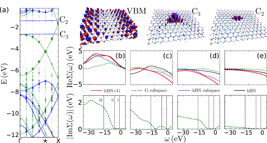
Figure 3: Excitations in an hBN-graphene heterostructure containing a nitrogen vacancy. (a) Calculated band structure – the states localized on graphene are in green, while blue points represent hBN. Lines serve as a guide for the eyes. The individual isosurfaces are shown on the right for VBM, $C_{3}$ defect state, and $C_{2}$ defect states. Second row contains averaged self-energy curves of the: (b) VBM, (c) $C_{3}$ defect state, (d) $C_{2}$ defect state, (e) CBM. Solid red lines are the full heterostructure self-energies; green and blue dashed lines are respectively the $\Sigma^{s}_{P}(\omega)$ graphene monolayer and hBN monolayer subspace self-energies. The black line represents the self-energy of an isolated hBN monolayer with $V_{N}$. The third row of panels contains the $\mathrm{Im}\Sigma^{s}_{P}(\omega)$ of graphene. Dashed vertical lines indicate the features in the experimental EELS spectrum from Ref. Kinyanjui et al., 2012. The experimentally observed features, labeled as i, ii, and iii, are attributed to $\pi\rightarrow\pi*$ interband transitions, $\pi$, and $\pi+\sigma$ plasmon excitations, respectively.

Due to the charge transfer and Fermi level shift, it is clear that graphene is responsible for altering the charge fluctuations, i.e., the polarization part of the self-energy. In practice, graphene acts as a dielectric background inducing a significant screening of the Coulomb interaction in hBN. It stands to reason that the localized defect states would be strongly affected by such a polarizable layer and that the corresponding self-energy should be dominated by the spectral features originating in graphene.

To investigate the degree of coupling and the contribution to the self-energy from each monolayer, we compute $\Sigma^{s}_{P}(\omega)$ using Eq. (22). Here, the $\{\phi\}$-subspace is constructed from stochastic samples of the 576 occupied graphene states (distinguished by green color in Fig. 3). For each sampling of the Green’s function, the subspace is described by eight random vectors in the $\{\phi\}$-subspace. Additional eight vectors sample the complementary subspace.

Fig. 3 shows the decomposition of the self-energy, indicating the contribution of graphene. For the delocalized states, the $\Sigma_{P}(\omega)$ curves appear similar to those in the hBN monolayer. Specifically, we see that $\Sigma_{P}(\omega)$ for VBM has practically identical frequency dependence between -15 and 0 eV. While in-plane contributions from hBN dominate the entire curve, screening from the graphene substrate is significant. A naïve comparison between the monolayer hBN and the heterostructure suggests that the enhanced maximum in Re$\Sigma_{P}$ at $-25$ eV is caused extrinsically by graphene. Surprisingly, this is not the case, and the effect is only indirect: the presence of graphene leads to shifting of the hBN spectral features. At the QP energy, graphene contributes to the correlation by $36\%$.

The situation is different for CBM. Towards the static limit ($\omega\to 0$), the self-energy curve becomes more negative. This shift is caused directly by the induced density fluctuations in the graphene substrate. The decreased polarization self-energy indicates the stabilization of the conduction states, which is directly linked to the attractive van der Waals fluctuations in bilayer systems.Brooks et al. (2020)

The self-energy curves of the $C_{3}$ and $C_{2}$ defect states are significantly different from those computed for the monolayer. In both cases, we observe a negative shift related to the QP stabilization by non-local correlations. The $\Sigma_{P}$ contributions to the defects’ QP energies are roughly three times larger in the heterostructure. Naïvely, we expect that the localized states are strongly coupled to graphene polarization modes, which lead to negative $\Sigma_{P}$. Surprisingly, the intrinsic hBN interactions are the major driving force. The defect states are mostly affected by the in-plane induced density fluctuations (constituting $64\%$ and $76\%$ of the total polarization self-energy for $C_{3}$ and $C_{2}$). Like the VBM, graphene indirectly acts on the defect QP states by enhancing the in-plane fluctuations, rather than direct coupling to the defects.

For all the states illustrated in Fig. 3, the graphene subspace contributions are governed by density oscillations induced by electron removal from or addition to the hBN layer. Collective charge excitations, i.e., plasmons, naturally correspond to the most prominent features. They are the poles of the screened Coulomb interaction and appear as strong peaks in the imaginary part of the subspace self-energy (bottom panels in Fig. 3).

Conceptually, the substrate plasmons are directly related to QP energy dissipation. Due to the weak coupling between the monolayers, Im$\Sigma_{P}^{s}(\omega)$ of the substrate shows the same spectral features at the experimental electron energy loss spectra measured for graphene alone. As distinct states couple to individual plasmon modes differently, the intensity of peaks in Im$\Sigma_{P}^{s}(\omega)$ varies. Due to changes in geometry and the presence of hBN, the spectral features are shifted from the experimental data. Still, we identify $\pi+\sigma$ and $\pi$ plasmons. The former is universally the most prominent feature in the subspace self-energy. The $\pi$ (possibly together with $\pi\to\pi^{*}$) plasmon contributes much less, and it is appreciable only for the $C_{3}$ defect state. We surmise that the additional peak near zero frequency corresponds to the “static” polarization of graphene due to the charge transfer from the defect.

As shown in this example, the stochastic subspace self-energy efficiently probes dynamical electron-electron interactions at interfaces. The random sampling allows selecting an arbitrary subspace to identify its contribution to the correlation energy and the excited state lifetimes.

VI Conclusions

Stochastic Green’ s function approaches represent a class of low-scaling many-body methods based on stochastic decomposition and random sampling of the Hilbert space. The overall computational cost is impacted by the presence of localized states that increase the sampling errors. Here, we have introduced a practical solution for the $G_{0}W_{0}$ method. The localized states are treated explicitly (deterministically), while the rest is subject to stochastic sampling. We have further shown that the subspace-separation can be applied to decompose the dynamical self-energy into contributions from distinct states (or parts of the systems).

Using nitrogen vacancy in hBN monolayer, we demonstrate that the deterministic embedding dramatically reduces the statistical fluctuations. Consequently, the computational time decreases by more than an order of magnitude for a given target level of stochastic error. The embedding is made within the Green’s function and the screened Coulomb interactions independently or simultaneously; the latter provides the best results. For delocalized states, embedding is not necessary and performs similar to the standard uniform sampling with real-space random vectors. The embedding scheme presented here is general, and it is the first step towards hybrid techniques that treat selected subspace at the distinct (higher) level of theory. The development of hybrid techniques is currently underway.

We further demonstrate that the subspace self-energy contains (in principle additive) contributions from the induced charge density. The self-energy contribution from a particular portion of the system is computed by confining sampling vectors into different (orthogonal) subspaces. We exemplify the capabilities of such calculations on defects state in the hBN-graphene heterostructure. Here, the charged excitation in one layer directly couples to density oscillations in the substrate monolayer. The response is dominated by plasmon modes, which are identified as features in the imaginary part of the subspace self-energy. Surprisingly, the electronic correlations for the defects are governed by the interactions in the host layer; the substrate only indirectly affects their strength.

This example serves as a stimulus for additional study of the defect states in heterostructures. Here, the coupling strength between individual subsystems is tunable by particular stacking order and induced strains. The subspace self-energy represents a direct route to explore such quantum many-body interfacial phenomena.