Abstract

Transformers are one of the most important machine learning workloads today. Training one is a very compute-intensive task, often taking days or weeks, and significant attention has been given to optimizing transformers. Despite this, existing implementations do not efficiently utilize GPUs. We find that data movement is the key bottleneck when training. Due to Amdahl’s Law and massive improvements in compute performance, training has now become memory-bound. Further, existing frameworks use suboptimal data layouts. Using these insights, we present a recipe for globally optimizing data movement in transformers. We reduce data movement by up to 22.91% and overall achieve a 1.30$\times$ performance improvement over state-of-the-art frameworks when training a BERT encoder layer and 1.19$\times$ for the entire BERT. Our approach is applicable more broadly to optimizing deep neural networks, and offers insight into how to tackle emerging performance bottlenecks.

1 Introduction

⬇

@dace.program

def mha_forward(

wq: dace.float16[P, H, I], bq: dace.float16[P, H],

q: dace.float16[I, B, J],

wk: dace.float16[P, H, I], bk: dace.float16[P, H],

k: dace.float16[I, B, K],

wv: dace.float16[W, H, I], bv: dace.float16[W, H],

v: dace.float16[I, B, K],

wo: dace.float16[W, H, I], bo: dace.float16[I],

scaler: dace.float16

):

qq = np.einsum("phi,ibj->phbj", wq, q) + bq[:,:,None,None]

kk = np.einsum("phi,ibk->phbk", wk, k) + bk[:,:,None,None]

vv = np.einsum("whi,ibk->whbk", wv, v) + bv[:,:,None,None]

beta = scaler * np.einsum("phbk,phbj->hbjk", kk, qq)

alpha = dropout(softmax(beta))

gamma = np.einsum("whbk,hbjk->whbj", vv, alpha)

out = np.einsum("whi,whbj->ibj", wo, gamma)+bo[:,None,None]

return out

(a) Input Code

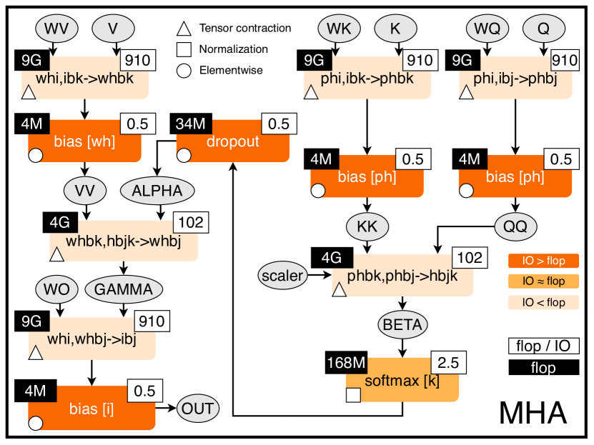
(b) Resulting dataflow

Figure 1: Input code and stateful dataflow multigraph (SDFG) for Multi-Head Attention. Throughout the paper, if not stated otherwise, the values are given for the following set of parameters: $P=W=64$, $H=16$, $I=P\cdot H=1024$, $B=8$, $J=K=512$. P/W: key/value projection size; H: # heads; I: embedding size; B: batch size; J/K: input/output sequence length.

Transformers Vaswani et al. (2017) are a class of deep neural network architecture for sequence transduction Graves (2012), with similar applicability as RNNs Rumelhart et al. (1986) and LSTMs Hochreiter & Schmidhuber (1997). They have recently had a major impact on natural language processing (NLP), including language modeling Radford et al. (2018); Wang et al. (2018; 2019), question-answering Rajpurkar et al. (2018), translation Vaswani et al. (2017), and many other applications. The significant improvement in accuracy brought by transformers to NLP tasks is comparable to the improvement brought to computer vision by AlexNet Krizhevsky et al. (2012) and subsequent convolutional neural networks. Transformers have also begun to be applied to domains beyond NLP, including vision Dosovitskiy et al. (2020), speech recognition Yeh et al. (2019), reinforcement learning Parisotto et al. (2019), molecular property prediction Maziarka et al. (2020), and symbolic mathematics Lample & Charton (2019).

Training transformers is very compute-intensive, often taking days on hundreds of GPUs or TPUs Devlin et al. (2019); Yang et al. (2019); Liu et al. (2019); Keskar et al. (2019); Shoeybi et al. (2019); Lan et al. (2019); Raffel et al. (2019). Further, generalization only improves with model size Radford et al. (2019); Shoeybi et al. (2019); Raffel et al. (2019); Microsoft (2020b), number of training samples Raffel et al. (2019); Liu et al. (2019), and total iterations Liu et al. (2019); Kaplan et al. (2020). These all significantly increase compute requirements. Indeed, transformers are becoming the dominant task for machine learning compute where training a model can cost tens of thousands to millions of dollars and even cause environmental concerns Strubell et al. (2019). These trends will only accelerate with pushes toward models with tens of billions to trillions of parameters Microsoft (2020b; c), their corresponding compute requirements OpenAI (2018), and increasing corporate investment towards challenges such as artificial general intelligence OpenAI (2019). Thus, improving transformer performance has been in the focus of numerous research and industrial groups.

Significant attention has been given to optimizing transformers: local and fixed-window attention Bahdanau et al. (2014); Luong et al. (2015); Shen et al. (2018); Parmar et al. (2018); Tay et al. (2019), more general structured sparsity Child et al. (2019), learned sparsity Correia et al. (2019); Sukhbaatar et al. (2019); Tay et al. (2020), and other algorithmic techniques Lan et al. (2019); Kitaev et al. (2020) improve the performance of transformers. Major hardware efforts, such as Tensor Cores and TPUs Jouppi et al. (2017) have accelerated tensor operations like matrix-matrix multiplication (MMM), a core transformer operation. Despite this, existing implementations do not efficiently utilize GPUs. Even optimized implementations such as Megatron Shoeybi et al. (2019) report achieving only 30% of peak GPU floating point operations per second (flop/s).

We find that the key bottleneck when training transformers is data movement. Improvements in compute performance have reached the point that, due to Amdahl’s Law and the acceleration of tensor contractions, training is now memory-bound. Over a third (37%) of the runtime in a BERT training iteration is spent in memory-bound operators: While tensor contractions account for over 99% of the arithmetic operations performed, they constitute only 61% of the runtime. By optimizing these, we show that the overhead of data movement can be reduced by up to 22.91%. Further, while MMM is highly tuned by BLAS libraries and hardware, we also find that existing frameworks use suboptimal data layouts. Using better layouts enables us to speed up MMM by up to 52%. Combining these insights requires moving beyond peephole-style optimizations and globally optimizing data movement, as selecting a single layout is insufficient. Overall, we achieve at least $1.30\times$ performance improvements in training over general-purpose deep learning frameworks, and $1.08\times$ over DeepSpeed Microsoft (2020a), the state of the art manually-tuned implementation of BERT. For robustly training BERT Liu et al. (2019), this translates to a savings of over $85,000 on AWS using PyTorch. For the GPT-3 transformer model Brown et al. (2020) with a training cost of $12M Wiggers (2020), our optimizations could save $3.6M and more than 120 MWh energy. To go beyond this, we develop a recipe for systematically optimizing data movement in DNN training.

Our approach constructs a dataflow graph for the training process, which we use to identify operator dependency patterns and data volume. With this representation, we identify opportunities for data movement reduction to guide optimization. We aim to maximize data reuse using various forms of fusion. Then we select performant data layouts, which is particularly impactful for normalization and tensor contraction operators, where it provides opportunities for vectorization and different tiling strategies. The performance data gathered is then used to find operator configurations that produce an optimized end-to-end implementation.

We evaluate these implementations first for multi-head attention, a core primitive within transformers and one that has significant applications beyond transformers Bello et al. (2019); Parmar et al. (2019); Cordonnier et al. (2020). We then consider the encoder layer from BERT Devlin et al. (2019), a widely-used transformer architecture. In each case, we compare against existing highly optimized implementations to provide strong baselines. Using this recipe, we are able to demonstrate significant performance improvements in both microbenchmarks and end-to-end training, outperforming PyTorch Paszke et al. (2019), TensorFlow+XLA Abadi et al. (2015), cuDNN Chetlur et al. (2014), and DeepSpeed Microsoft (2020a). While we focus our work on particular transformer models, our approach is generally applicable to other DNN models and architectures. We summarize our contributions as follows:

• We find transformer training to be memory-bound and significantly underperforming on GPUs.

• We develop a generic recipe for optimizing training using dataflow analyses.

• Using this recipe, we systematically explore performance of operators and the benefits of different optimizations.

• We demonstrate significant performance improvements, reducing data movement overheads by up to 22.91% over existing implementations, and achieving at least $1.08\times$ performance improvements over specialized libraries, and $1.30\times$ over general-purpose frameworks.

• We make our code publicly available at https://github.com/spcl/substation.

2 Background

Here we provide a brief overview of our terminology, transformers, and data-centric programming. We assume the reader is generally familiar with training deep neural networks (see Goodfellow et al. (2016) for an overview) and transformers (see Sec. A.1 for a more complete overview).

2.1 Transformers

We use the standard data-parallel approach to training, wherein a mini-batch of samples is partitioned among many GPUs. During backpropagation, we distinguish between two stages: computing the gradients with respect to a layer’s input ($dX$), and computing the gradients with respect to the layer’s parameters ($dW$). Note that the second stage is relevant only for layers with learnable parameters.

Figure 2: Forward and backpropagation for a BERT-large encoder layer, and the ratio of flop to memory accesses (words) when training on a batch $B=8$ and sequence length $J=K=512$.

The transformer architecture Vaswani et al. (2017) consists of two main components: multi-head attention (MHA) and a feed-forward network. We provide Python code and an illustration of MHA forward propagation in Fig. 1. Attention has three input tensors, queries (q), keys (k), and values (v). The inputs are first multiplied by weight tensors wq, wk, wv, respectively, as a learned input projection (we use Einstein-notation sums, or einsums, for tensor contractions). The query and key tensors are subsequently multiplied together and scaled (stored in beta), followed by a softmax operation. This is then multiplied with vv to produce the per-head output (gamma). The outputs of all heads are finally concatenated and linearly projected back to the input dimension size (i).

The respective dataflow graph (Fig. 1(b)) immediately exposes coarse- (whole graph) and fine-grained (within rectangular nodes) parallelism, as well as data reuse. As every edge represents exact data movement, their characteristics (access sets and movement volume) can be inspected for bottlenecks and potential solution analysis.

We focus on BERT Devlin et al. (2019). Fig. 2 illustrates the forward and backward pass for a single BERT encoder layer. The layer essentially consists of MHA followed by a feed-forward neural network (two linear layers with bias and ReLU activations after the first layer). Dropout Srivastava et al. (2014), layer normalization Ba et al. (2016), and residual connections He et al. (2016) are also used.

2.2 Data-Centric Programming

As DNN processing is among the most popular compute-intensive applications today, considerable efforts have been made to optimize its core operators Ben-Nun & Hoefler (2019). This has driven the field to the point where optimization today is almost exclusively performed beyond the individual operator, either on the whole network Google (2020); PyTorch Team (2020) or repeated modules.

Performance optimization on modern architectures consists of mutations to the original code, sometimes algorithmic Chellapilla et al. (2006); Mathieu et al. (2013); Lavin & Gray (2016) but mostly relating to hardware-specific mapping of computations and caching schemes. This includes tiling computations for specific memory hierarchies, using specialized units (e.g., Tensor Cores) for bulk-processing of tiles, modifying data layout to enable parallel reductions, hiding memory latency via multiple buffering, pipelining, and using vectorized operations. It is thus apparent that all current optimization techniques revolve around careful tuning of data movement and maximizing data reuse.

The Data-Centric (DaCe) parallel programming framework Ben-Nun et al. (2019) enables performance optimization on heterogeneous architectures by defining a development workflow that enforces a separation between computation and data movement. The core concept powering program transformation is the Stateful Dataflow multiGraph (SDFG), a graph intermediate representation that defines containers and computation as nodes, and data movement as edges. DaCe takes input code written in Python or DSLs, and outputs corresponding SDFGs. Programmers can mutate the dataflow via user-extensible graph-rewriting transformations to change the schedule of operations, the layout of data containers, mapping of data and computation to certain processing elements, or any adaptation to the data movement that does not change the underlying computation.

As opposed to traditional optimizing compilers and deep learning frameworks (e.g., XLA, TorchScript), DaCe promotes a white-box approach for performance optimization. The framework provides an API to programmatically instrument and explore, e.g., layouts and kernel fusion strategies, without modifying the original code. DaCe can map applications to different hardware architectures, including CPUs, GPUs, and FPGAs Ben-Nun et al. (2019), enabling both whole-program and micro-optimizations of nontrivial applications to state-of-the-art performance Ziogas et al. (2019).

The combination of the separation of the algorithm from the transformed representation and white-box approach for optimization enables us to inspect and optimize the data movement characteristics of Transformer networks. As we shall show in the next sections, this drives a methodical approach to optimizing a complex composition of linear algebraic operations beyond the current state of the art.

3 Optimizing Transformers

We now apply our recipe to optimize data movement in training, using a BERT encoder layer as an example. We focus on a single encoder layer, since these are simply repeated throughout the network, and other components (e.g., embedding layers) are not a significant component of the runtime. In this section, we discuss dataflow and our operator classification. Sections 4 and 5 discuss our optimizations and Section 6 presents end-to-end results for transformers.

At a high level, our recipe consists of the following steps:

1. Construct a dataflow graph for training and analyze the computation to identify common operator classes.

2. Identify opportunities for data movement reduction within each operator class using data reuse as a guide.

3. Systematically evaluate the performance of operators with respect to data layout to find near-optimal layouts.

4. Find the best configurations to optimize end-to-end performance of the training process.

3.1 Dataflow Analysis

We use SDFGs and the DaCe environment to construct and analyze dataflow graphs. Fig. 2 provides a simplified representation of dataflow in a transformer encoder layer. Each node represents an operator, which is a particular computation along with its associated input and output, which may vary in size. An operator may be implemented as multiple compute kernels, but is logically one operation for our analysis. To produce an SDFG, all that is required is a simple implementation using NumPy. As the goal of this stage is to understand the dataflow, we do not need to optimize this implementation: It is simply a specification of the computations and data movement.

Using DaCe, we can estimate data access volume and the number of floating point operations (flop) required for each computation. Fig. 2 is annotated with flop and the ratio of flop to data volume, and we provide a precise comparison with PyTorch in Tab. A.1. The key observation is that the ratio of data movement to operations performed varies significantly among operators. In many cases, the runtime of an operator is dominated by data movement, rather than computation, and this should be the target for optimization.

3.2 Operators in Transformers

Table 1: Proportions for operator classes in PyTorch.

Operator class	% flop	% Runtime
$\medtriangleup$ Tensor contraction	99.80	61.0
$\largesquare$ Stat. normalization	0.17	25.5
$\medcircle$ Element-wise	0.03	13.5

With this analysis, we can now identify high-level patterns that allow us to classify operators. We base our classification both on the data movement to operation ratio and the structure of the computations. This classification is useful as it allows us to consider optimizations at a more general level, as opposed to working on each operator (or kernel) individually. For transformers, we find three classes: tensor contractions, statistical normalizations, and element-wise operations. The border of each operator in Fig. 2 indicates its class and Tab. 1 gives the proportion of flop and runtime for a BERT encoder layer for each class.

Tensor Contractions $\medtriangleup$ These are matrix-matrix multiplications (MMMs), batched MMMs, and in principle could include arbitrary tensor contractions. We consider only MMMs and batched MMMs for simplicity, as these are efficiently supported by cuBLAS. In transformers, these are linear layers and components of MHA. These operations are the most compute-intensive part of training a transformer. For good performance, data layout and algorithm selection (e.g., tiling strategy) are critical.

Statistical Normalizations $\largesquare$ These are operators such as softmax and layer normalization. These are less compute-intensive than tensor contractions, and involve one or more reduction operation, the result of which is then applied via a map. This compute pattern means that data layout and vectorization is important for operator performance.

Element-wise Operators $\medcircle$ These are the remaining operators: biases, dropout, activations, and residual connections. These are the least compute-intensive operations.

3.3 Memory Usage Efficiency (MUE)

The MUE metric Fuhrer et al. (2018) provides a measure of the memory efficiency of an operation, both with respect to its implementation and achieved memory performance. This provides another method for understanding performance beyond flop/s that is particularly relevant for applications that are bottlenecked by data movement. MUE evaluates the efficiency of a particular implementation by comparing the amount of memory moved ($D$) to the theoretical I/O lower bound Jia-Wei & Kung (1981) ($Q$) and the ratio of achieved ($B$) to peak ($\hat{B}$) memory bandwidth: $\textrm{MUE}=\nicefrac{{Q}}{{D}}\cdot\nicefrac{{B}}{{\hat{B}}}\cdot 100$. If an implementation both performs the minimum number of operations and fully utilizes the memory bandwidth, it achieves $\textrm{MUE}=100$. This can be thought of as similar to the percent of peak memory bandwidth.

3.4 Evaluation Details

We use the Lassen supercomputer Livermore Computing Center (2020), where each node has four 16 GB Nvidia V100 GPUs with NVLINK2. For comparison, we use cuDNN 8.0.4, PyTorch 1.6.0 (PT), TensorFlow 2.1 from IBM PowerAI with XLA, and a recent development version of DeepSpeed (DS). See Sec. A.3 for more details. Our running example is training BERT-large. We use a mini-batch size of $B=8$, sequence length $L=512$, embedding size $N$=$1024$, $H$=$16$ heads, and a projection size $P=64$.

4 Fusion

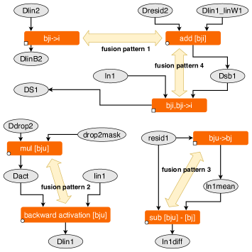
Figure 3: Examples of operator fusion.

A significant portion of the runtime in existing transformer implementations is in statistical normalization and element-wise operators (Tab. 1). Thus, fusion is a major opportunity for promoting data reuse, as when operators cover identical iteration spaces, global memory writes and subsequent reads between them can be removed.

We develop a set of fusion rules applicable to any application with operators similar to the three here. The process consists of two steps: detecting which operations can be fused and then deciding whether it is beneficial to fuse them.

To discover fusion opportunities, we analyze iteration spaces. Every operator has independent dimensions. Statistical normalization operators also have reduction dimensions; tensor contractions also have reduction dimensions and special independent dimensions for the two input tensors.

The type of iteration space implementation determines which tools are used to make them. Independent dimensions can be implemented using GPU block or thread parallelism, or "for" loops within a single thread. Reduction dimensions use these techniques but also specify how the reduction is to be performed: accumulating to the same memory location ("for" loops), or as grid-, block-, or warp-reductions.

Two operators can be fused if their iteration space implementations are compatible: They are either the same or the only difference is that one operator performs a reduction. The order and size of dimensions and the implementation for each must match. If the first operator produces output the second uses as input, partial fusion can be done: The outermost independent dimensions can be shared, but the innermost iteration spaces are put in sequential order inside.

When a fusion opportunity is detected, we take it in two cases: First, if we can perform fewer kernel launches by merging iteration spaces. Second, if we achieve less data movement by avoiding loads and stores between operators. Theoretically, the first case could increase memory pressure, but we observe it provides benefits in practice.

We attempt to fuse maximally. There are four structural patterns (Fig. 3) in the dataflow graph for the encoder layer when fusion rules above are applied to a pair of non-tensor contraction operators. Using the SDFG, we fuse two adjacent operators whenever we detect these patterns and continue until we cannot fuse further. This means we fuse until either a reduction dimension or iteration space changes. As a further constraint, we only fuse simple element-wise scaling operations into tensor contraction operators.

Each fused operator is implemented as a CUDA kernel specialized for a specific data layout. Due to space limitations, we detail our implementation and fused kernels in Sec. A.2.

4.1 Results

Tab. A.1 presents our comprehensive results, including operator fusion. In this, we show a detailed breakdown of the required and observed flop, data movement, runtime, and MUE for each operator within the encoder layer, for both PyTorch and our implementation, with our fused operators marked. We can easily observe that while the vast majority of flop are in tensor contractions, much of the runtime is in statistical normalization and element-wise operators (see also Tab. 1). These operators are indeed memory-bound.

In forward propagation, every fused operator outperforms PyTorch’s. In backpropagation, this trend generally holds, but ebsb and baob are slower due to our configuration selection algorithm choosing a suboptimal layout for some operators to optimize the overall performance (see Sec. 6).

By studying the MUE and flop/s, we can reason about the bottlenecks behind each operator. For the fused operators, we see that high MUE rates are often achieved. In fact, the MUE from Tab. A.1 and the theoretical flop/IO ratio from Fig. 2 are highly correlated across operators. We say that a kernel is memory bound if its MUE is larger than the achieved peak flop/s, and compute bound otherwise. This insight aids in analyzing the bottlenecks of general DNNs and automated tuning of operators, prior to measuring their performance. We note that for our operators, which involve multiple tensors of different shapes, 100% MUE is potentially unattainable as achieving peak memory bandwidth requires a highly regular access pattern into DRAM.

As for the tensor contraction results, we see that the attained MUE is consistently under 50%. This is acceptable, since the underlying matrix multiplications are generally compute-bound. However, we note that some cases, such as $QK^{T}$, are both low in flop/s and MUE. A more in-depth look into the dimensions of the contraction reveals that the dimensions are small, which then indicates that the tensor cores are underutilized. This may result from insufficient scheduled threads, or low memory throughput to compute ratio. We thus try to increase hardware utilization by fusing additional operators into the contractions next.

Additional Fusion Approaches We considered two additional fusion approaches, fusing operators into tensor contractions and algebraic fusion, which we discuss in Sec. A.5 due to limited space. We find that fusing into tensor contractions is not profitable, but algebraic fusion to combine input projection operations in MHA is.

5 Data Layout

We now consider data layout selection, which enables efficient access patterns, vectorization, and tiling strategies for tensor contraction and statistical normalization operators. To study this systematically, for each operator, including fused operators produced in the prior step, we benchmark every feasible data layout, as well as varying other parameters depending on the specific operator. The best parameterization of an operator is highly dependent on the GPU model and tensor sizes, and may not be obvious a priori; hence it is important to consider this empirically.

Because there are a myriad of potential configurations for each operator, we summarize the distribution of runtimes over all configurations using violin plots. The width of the violin represents the relative number of configurations with the same runtime. This allows us to see not only the best runtime but sensitivity of operators to layouts, an important factor for global layout optimization in Step 4 of our recipe.

5.1 Tensor Contractions

Using the Einsum notation for tensor contractions, we consider all equivalent permutations of the summation string. The einsum is then mapped to a single cuBLAS MMM or batched MMM call. While this notation allows us to express arbitrary tensor contractions, as cuBLAS does not support all configurations, we limit ourselves to these two types.

In addition, we consider every possible cuBLAS algorithm for each layout, as we have observed that the heuristic default selection is not always optimal. We use the cublasGemmEx API to manually select algorithms. We use both regular and Tensor Core operations, and perform all accumulations at single-precision, in line with best practices for mixed-precision training Micikevicius et al. (2018).

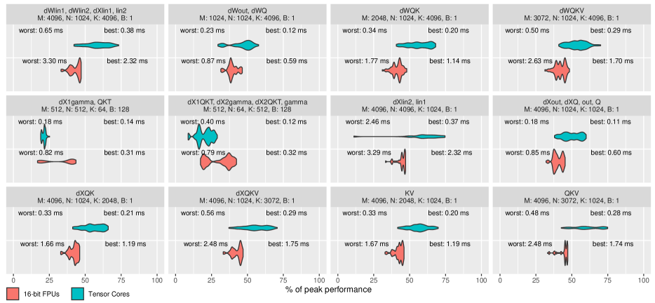
Figure 4: Tensor contraction performance. Tensor Core peak: 125 Tflop/s; FP16 peak: 31.4 Tflop/s.

Fig. 4 presents performance distributions over all data layouts for every tensor contraction in the encoder layer training, including algebraic fusion variants. Each plot is for different tensor sizes and shows the performance with and without Tensor Cores. Since input matrices for cuBLAS MMMs can be easily swapped, results for both orders are merged into the plot and labeled with $M>N$. Interestingly, in several cases (where $N$ or $K$ is 64) the performance is quite close to the regular floating point units, due to a failure to saturate the tensor cores. Among the tensor core results, we can typically see there are several modes in the performance distributions; these correspond to particularly important axes for data layout. Indeed, for many configurations, one of these is near to or contains the best-performing configuration, indicating that many slightly different data layouts could be used with little impact on performance depending on the needs of our global optimization pass. However, this does not mean that any data layout is acceptable; in every case, the majority of the layouts do not perform well, illustrating the importance of careful tuning.

We also investigated how the default cuBLAS algorithm compares to the best-performing configuration. On half precision, we found that the algorithm chosen by cuBLAS’s heuristic was up to 14.24% worse than the best algorithm (in $dX1\,QK^{T}$). We also investigated the performance at single-precision and found similar results with up to 7.18% worse performance. This demonstrates the importance of tuning for particular hardware and workload.

5.2 Fused Operators

For our fused operators, we consider all combinations of input and output layout permutations. This enables us to include transposes of the output data as part of the operator, should the next operator perform better in a different layout than the input. The data layout is especially critical for statistical normalization operators, where the appropriate data layout can enable vectorization opportunities, especially vectorized loads and stores for more efficient memory access. We therefore also consider vectorization dimensions, the mapping of dimensions to GPU warps, etc. Our implementation takes advantage of these layouts when feasible.

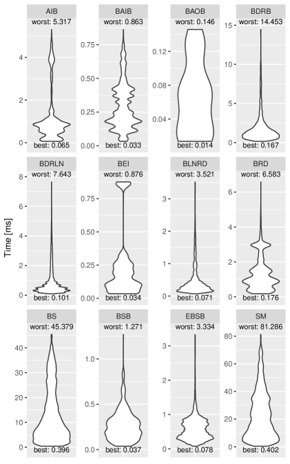
Figure 5: Performance of fused kernels for element-wise and statistical normalization operators.

Fig. 5 presents the runtime distribution for all configurations of our fused operators (note that some are used twice; see Sec. A.2 for details of each operator). The distributions here are qualitatively similar to those in Fig. 4, except these have much longer tails: A bad configuration is, relatively, much worse, potentially by orders of magnitude.

All kernels support changing the layouts of tensors they use. This change is done via template parameterization, so the compiler can generate efficient code. All kernels support selecting different vectorization dimensions. The brd and bei kernels can select the dimension used for CUDA thread distribution; bsb, ebsb, and bdrb can select the warp reduction dimension, as they reduce over two dimensions.

The most noticeable performance improvement is made by layouts that enable vectorized memory access, showing that the main performance limitation is the amount of moved data. The second notable category are layouts with the same reduce and vector dimensions. Joining these dimensions decreases the number of registers required to store partially reduced values from the vector size (eight at FP16) to one.

We can expect to get good performance restricting ourselves to configurations in the two groups described above. Usually, the best layout discovered follows them. For example, the sm kernel has the same warp and reduction dimensions, and these dimensions are the last and sequential ones for involved arrays. However, this intuition is not always correct. From the results in Fig. 5, we find that there are configurations that both satisfy these intuitive rules yet are very slow. For example, the best configuration of aib takes 65 $\mu$s, and the worst "intuitively good" configuration takes 771 $\mu$s.

Configurations discovered through exhaustive search can enhance our intuitive understanding of what is required for good performance. For example, the brd kernel uses four 3D tensors, which can use six possible layouts. Intuitively, we want to place the vectorized dimension last to make it sequential for all tensors. Surprisingly, however, the best configuration has only two tensors vectorized. With this information, intuition can be refined: the likely factor that limits vectorization over all tensors is excessive register usage. However, unlike the exhaustive search, intuition does not help to identify which tensors to vectorize.

6 End-to-End Optimization

The final step is to assemble fused components and select data layouts for each operator to yield a complete implementation. This is the culmination of the prior steps performing dataflow analysis, fusion, and layout selection. From these, we have performance data for all data layouts and algebraic fusion strategies. One cannot simply pick a single layout a priori, as the benefit of running two operators in different layouts may outweigh the overhead of transposing data. Our assembled implementation is structured using the SDFGs produced in Step 1. We integrate it into PyTorch Paszke et al. (2019) via its C++ operator API.

6.1 Configuration Selection

We develop an automatic configuration selection algorithm to globally optimize our implementation using the performance data. We construct a directed graph (Fig. 6) based on the dataflow graph of the operators. Beginning from the input data and proceeding in a topological order, we add a node to the graph for each input and output data layout of the operator. An edge is added from the input to the output layout, weighted with the minimum runtime of any configuration with that layout. Determining this simply requires a linear search over the matching performance data. This allows us to select both the best data layout and any other operator knobs (e.g., vectorization dimension). To minimize the size of the graph, we only add a configuration from an operator when it has at least one input and output edge. We then run a single-source shortest-path (SSSP) algorithm from the input to the output in the graph; the resulting path gives our final configuration. Because this graph is a DAG and the number of feasible input/output configurations for each operator is small, SSSP takes linear time asymptotically and seconds for BERT. The path is saved to a configuration file which is used to automatically define tensor layouts at the start of training.

Figure 6: Example configuration selection graph for SSSP.

To simplify the implementation, we omit dataflow connections between forward and backpropagation operators. This assumption could be relaxed in a future version of this algorithm. Although this means we are not guaranteed to find a globally optimal data layout, the runtime of our configuration is nevertheless within 6% of an ideal (incorrect) layout configuration that ignores data layout constraints.

6.2 Multi-head Attention

We first analyze the performance of multi-head self-attention. While it is a key primitive in BERT, MHA is also used outside of transformers, so understanding its performance in isolation can inform other models too. Tab. 2 compares our globally-optimized implementation with PyTorch, TensorFlow+XLA, and cuDNN. cuDNN’s MHA implementation (cudnnMultiHeadAttnForward and related) supports six data layouts; we report the fastest.

cuDNN’s performance is significantly worse than the others; as it is a black box, our ability to understand it is limited. However, profiling shows that its implementation launches very large numbers of softmax kernels, which dominate the runtime, indicating additional fusion would be profitable. TensorFlow+XLA finds several fusion opportunities for softmax. However, its implementation does not perform algebraic fusion for the queries, keys, and values, and it uses subpar data layouts for tensor contractions.

Our performance results in Tab. A.1 illustrate the source of our performance advantage over PyTorch: Our data layout and algorithm selection results in faster tensor contractions overall. This is despite the Gamma stage actually being slower than PyTorch’s: Sometimes locally suboptimal layouts need to be selected to improve performance globally.

Table 2: Multi-head attention performance for BERT.

	TF+XLA	PT	cuDNN	Ours
Forward (ms)	1.60	1.90	3.86	1.25
Backward (ms)	2.25	2.77	680	1.86

6.3 End-to-End Performance

We present overall performance results for the encoder layer in Tab. 3. For forward and backpropagation combined, we are $1.30\times$ faster than PyTorch and $1.20\times$ faster than TensorFlow+XLA, including framework overheads. At a high level, this is because we perform a superset of the optimizations used by both frameworks, and globally combine them to get all the advantages while minimizing drawbacks. As a general guideline, we use flop and MUE rates as proxies for which operators require the most attention and their corresponding bottlenecks. This ensures a guided optimization rather than tuning all operators aggressively.

We also include performance results from DeepSpeed, which we are $1.08\times$ faster than. This is despite DeepSpeed being a manually-optimized library tuned specifically for BERT on V100s. Note also that DeepSpeed modifies some operations, e.g., to be reversible or to exploit output sparsity, and so is not always strictly comparable to the other implementations. This also provides it opportunities for optimization that we do not consider.

The total data movement reduction we attain is $\sim$22.91% over the standard implementation. We obtain this information from Tab. A.1, where for each fused kernel we omit the interim outputs and inputs that are not part of the overall I/O that the fused kernels perform. TensorFlow+XLA’s automatic kernel fusion reduces data movement similarly to ours. However, the data layouts used for tensor contractions are not optimal, and its BERT encoder implementation does not use algebraic fusion in MHA. PyTorch’s data layouts enable faster tensor contractions and it implements the algebraic fusion, but it has higher overheads for other operators.

Our fusion pass finds all the opportunities that TF+XLA does, plus several additional ones; for example, we implement layernorm as a single fused kernel. Our data layout selection picks better layouts than PyTorch in nearly every individual instance; when it does not, this is because the layout change enables greater performance gains downstream. In Tab. A.1, we also see that PyTorch performs more flop than predicted. Some of this is due to padding in cuBLAS operations, and generic methods performing excess operations. However, we also discovered that some cuBLAS GEMM algorithms, including ones called by PyTorch, incorrectly perform twice as many FLOPs as necessary; our recipe avoids these cases automatically.

We also considered another configuration for training BERT, where we change the batch size to $B=96$ and the sequence length to $L=128$, and retuned our layout selection. In this case, forward and backpropagation for a single encoder layer takes 18.43 ms in PyTorch, 16.19 ms in DeepSpeed, and 15.42 ms in our implementation. We outperform both PyTorch and DeepSpeed in this case (even with its additional optimizations). We believe that with improvements to our layout selection algorithm, the performance of our implementation will improve further.

Finally, we performed end-to-end training of BERT at scale. We observe an overall speedup of $1.19\times$, despite additional training overheads. We show pretraining curves in Fig. 7 and present full details of the experiment in Sec. A.6.

Beyond BERT, other transformers have very similar layers, such as decoder layers in GPT-2/3. With very few changes, our recipe and implementations are directly applicable to these. Our implementation can also be extended to support a full training pipeline by stacking our optimized layers.

Table 3: Full BERT encoder layer performance.

	TF+XLA	PT	DS	Ours
Forward (ms)	3.2	3.45	2.8	2.63
Backward (ms)	5.2	5.69	4.8	4.38

Figure 7: Pretraining curve for BERT-large.

7 Related Work

We provide a brief overview of related work here, and a more comprehensive discussion in Sec. A.7.

Most directly relevant are other approaches specifically to accelerate transformer training. Distributed-memory techniques, such as ZeRO Rajbhandari et al. (2019), Megatron Shoeybi et al. (2019), and Mesh-TensorFlow Shazeer et al. (2018) scale training to many GPUs to accelerate it. Mesh-TensorFlow also presents a classification of operators similar to ours. Large batches have also been used to accelerate training via LAMB You et al. (2020) or NVLAMB NVIDIA AI (2019). None of these directly address the performance of a single GPU as done in this paper. DeepSpeed Microsoft (2020a), which we compare with in Section 6.3, is closest to our work, but performs all optimizations and layout selections manually.

Many frameworks provide optimizations that can also be applied to transformers, such as XLA or TVM Chen et al. (2018). None of these works provide all the optimizations or the systematic study of data movement and its impact on performance provided here. Beyond deep learning, data movement reduction is a core component of high-level optimization Unat et al. (2017) and polyhedral optimizations (e.g., Grosser et al. (2012)). Other white-box approaches for optimization exist (e.g., Halide Ragan-Kelley et al. (2013) and MLIR Lattner et al. (2020)). The data-centric optimization approach proposed here using dataflow graphs allows us to perform and tune complex data layout and fusion transformations that span granularity levels, surpassing the optimization capabilities of the aforementioned tools and achieving state-of-the-art performance.

8 Discussion

The recipe we propose in this paper can be directly adopted in other DNN architectures. Additional transformer networks, such as Megatron-LM Shoeybi et al. (2019) and GPT-3 Brown et al. (2020), only differ by dimensions and minor aspects in the encoder and decoder blocks (e.g., dropout position, biases). Once a data-centric graph is constructed from them, the recipe remains unchanged.

8.1 Beyond Transformers

The classification of operators into three groups covers a wide variety of operators that span beyond transformers.

Large tensors and their contraction are ubiquitous in modern DNNs. For MLPs and recurrent neural networks (RNNs), there is little change, as the core operator types are essentially the same. Convolutions, pooling, and other local spatial operators can be treated similarly to tensor contractions, owing to their arithmetic intensity properties and abundance of optimized implementations. Therefore, the same considerations we take here are just as critical in CNNs. However, as opposed to contractions (see Section A.5.1), further fusion is typically considered for convolutions.

Statistical normalization also takes different forms in DNNs. This includes a variety of reductions, as well as Instance, Group, and Batch Normalization, where the latter constitutes the second largest computation in ResNets after convolutions. When varying data layouts, these operators share properties (normalizing a dimension) and are optimized in exactly the same way. Lastly, element-wise operators always exist in DNNs and benefit from the same fusion and bulk data movement optimizations as we perform here. For graph neural networks Bronstein et al. (2017), capsule neural networks Sabour et al. (2017), and other emerging architectures, the operators change more significantly, but the basic procedure applies.

Due to the prohibitively large search space of configurations in transformers, writing manually-optimized kernels becomes infeasible. Instead, each of our data-centric implementations chooses an optimization scheme (e.g., tiling, vectorization, warp-aggregated reductions) automatically, according to the input data layout and the operator type. Combined with automated configuration selection (Section 6.1), we rely only on the dataflow graph structure to choose the best feasible data layout configuration.

8.2 Hardware Implications

The implications of data movement reduction extend beyond software. Given that the best performance for different operators is achieved with different data layouts, there would be significant benefits if future machine learning accelerators included built-in support for fast data layout changes. We confirm this in our MUE results (Tab. A.1), as even the most compute-intensive tensor contractions are bounded by the hardware’s capability of transferring data to Tensor Cores.

Hardware trends indicate a similar situation. New architectures are moving towards reducing data format conversion (e.g., TF32 Nvidia (2020)), increased on-chip memory and low-latency interconnects Jia et al. (2019c), and coarse-grained spatial hardware Cerebras (2020). For the latter two, the recipe and analysis provided here is crucial to maintain high utilization in pipelined DNN execution. More generally, we expect our recipe to be applicable to any load-store architecture (e.g., TPUs Jouppi et al. (2017)). The % of peak and MUE are fundamental quantities and analyzing them will allow one to study bottlenecks and optimize appropriately.

9 Conclusions

Despite the importance of transformer neural networks, training them is memory-bound and underutilizes GPUs. Using our recipe for data movement analysis, we identified bottlenecks and optimizations, yielding improved implementations that outperform the already highly tuned state-of-the-art. As training transformers is already a major workload that will only grow larger, our improvements offer significant real-world impacts for both research and industry.

Our approach is applicable more broadly to deep learning; many DNNs easily fit within our operator classification. This is especially important for guiding the optimization of emerging model architectures, which do not benefit from existing acceleration libraries. Our results also highlight the importance of considering data movement at every level of the training stack—from the application down to hardware.

Appendix A Supplementary Material

A.1 Additional Background

We use the standard data-parallel approach to training, wherein a mini-batch of samples is partitioned among many GPUs. During backpropagation, we distinguish between two stages: computing the gradients with respect to a layer’s input ($dX$), and computing the gradients with respect to the layer’s parameters ($dW$). Note that the second stage is relevant only for layers with learnable parameters.

A.1.1 Transformers

The transformer architecture Vaswani et al. (2017), originally developed for machine translation, is a neural network architecture for sequence transduction, or transforming an input sequence into an output sequence. Transformers build upon a long sequence of work within natural language processing, most relevantly beginning with word embeddings Mikolov et al. (2013c; a; b), neural machine translation Kalchbrenner & Blunsom (2013); Cho et al. (2014), and sequence-to-sequence learning Sutskever et al. (2014). A key component is attention Bahdanau et al. (2014); Luong et al. (2015), which enables a model to learn to focus on particular parts of a sequence.

The transformer makes two key contributions. First, it generalizes attention to multi-head attention, which we discuss below. Second, the transformer neglects recurrent or convolutional mechanisms for processing sequences, and relies entirely on attention. Critically, this enables significantly more parallelism during training, as the model can process every element of a sequence simultaneously, instead of having a serial dependence on the prior element.

A.1.2 Multi-head Attention

Multi-head attention (MHA) generalizes attention, and uses h attention “heads” in parallel to attend to different learned projections of a sequence. We provide Python code and an illustration of MHA forward propagation in Fig. 1.

Each attention head is an instance of scaled dot-product attention, with input tensors: queries (q), keys (k), and values (v). Conceptually, attention finds values corresponding to the keys closest to the input queries. Heads are augmented with learned linear layers that project their inputs into a lower-dimensional space. The three inputs are first multiplied by weight tensors wq, wk, wv, respectively, as a learned input projection (we use Einstein-notation sums, or einsums, for tensor contractions). The query and key tensors are subsequently multiplied together and scaled (stored in beta), followed by applying the softmax operation in order to weight and select the most important results. This is then multiplied with vv to produce the per-head output (gamma). The outputs of all heads are finally concatenated and linearly projected back to the input dimension size (i).

The respective dataflow graph (Fig. 1(b)) immediately exposes coarse- (whole graph) and fine-grained (within rectangular nodes) parallelism, as well as data reuse. As every edge represents exact data movement, their characteristics (access sets and movement volume) can be inspected for guided bottlenecks and potential solution analysis.

There are three broad classes of MHA, distinguished by their inputs. General attention uses distinct tensors as the queries, keys, and values. Encoder/decoder attention uses the same tensor for both keys and values. Self-attention uses the same tensor for all three inputs. MHA may also have a masking step, which is used during training to prevent a model from “seeing the future” and using information from a later part of a sequence.

A.1.3 Transformer Architectures

BERT Devlin et al. (2019) is a widely-used transformer for NLP tasks. Fig. 2 illustrates the forward and backward pass for a single BERT encoder layer. The layer essentially consists of MHA (as self-attention) followed by a feed-forward neural network (two linear layers with bias and ReLU activations after the first layer). Dropout Srivastava et al. (2014), layer normalization Ba et al. (2016), and residual connections He et al. (2016) are also used.

Transformers also incorporate several other layers that we will not discuss in detail: embedding layers for input sequences and various output layers, depending on the task. Other transformer architectures, such as the original Transformer and GPT-2/3 Radford et al. (2019); Brown et al. (2020) have very similar architectures.

A.2 Fusion Implementation

We implement each fused operator as a single custom CUDA kernel and specialize it for a specific data layout using templates to maximize opportunities for compiler optimization. To correctly handle data dependencies, if a reduction is the first operator in a fusion kernel, it is implemented with two loops: the first computes the reduction and the second uses it. Otherwise, each kernel is implemented as a single loop.

Reduction operations in statistical normalizations use a warp allreduce among all threads in a warp, implemented with CUDA intrinsics. If the number of elements to be reduced exceeds the warp size, we perform a sequential reduction over smaller chunks first. Layout-permuting, we use vectorized loads, stores, and arithmetic within a single thread, and fall back to word-wise implementations otherwise. For dropout operators, which must generate a random mask, we use cuRAND for random number generation.

After fusion, we have the following fused element-wise and normalization operations. Fig. 3 illustrates several cases.

• aib: Attention input bias.

• baob: Backward attention output bias.

• baib: Backward attention input bias.

• sm: Softmax with scaling and dropout.

• brd: Bias, ReLU, and dropout.

• bdrln: Bias, dropout, residual, and layernorm.

• bsb: Backward layernorm scale and bias.

• blnrd: Backward layernorm dX and dropout, saving the intermediate result for the residual connection.

• bdrb: Backward dropout, ReLU, and bias.

• ebsb: Backward residual and layernorm scale and bias.

• bs: Backward dropout and softmax with scaling.

• bei: Backward encoder input residual connection.

A.3 Evaluation Details

All our results were produced on the Lassen supercomputer Livermore Computing Center (2020), which consists of 795 nodes, each with two IBM Power9 CPUs and four Nvidia V100 GPUs with NVLINK2 and 16 GB of memory. We use CUDA 10.1.243 and GCC 7.3.1 to build our code. For comparison, we use cuDNN 7.6.5, PyTorch 1.6.0 (PT) (built-in transformer implementation), TensorFlow 2.1 from IBM PowerAI with XLA enabled (transformer adapted from Wolf et al. (2019)) (TF+XLA), and a recent development version of DeepSpeed (DS). Unless noted, our results use mixed-precision training Micikevicius et al. (2018), with FP16 data and accumulations performed at FP32. In PyTorch, we use Apex Nvidia (2020a) for mixed-precision; in TensorFlow and DeepSpeed, we use the built-in automatic mixed-precision. Results are the mean of 100 measurements. When we compute the percent of peak performance, we use the 125 Gflop/s Tensor Core peak on our V100s for tensor contraction operations, and the 31.4 Gflop/s half-precision peak for other operations.

A.4 Flop Analysis

Tab. A.1 presents our complete flop analysis. See Sec. 4.1 for details.

Table A.1: Flop analysis for BERT encoder layer. $\medtriangleup$ – tensor contraction, $\largesquare$ – statistical normalization, $\medcircle$ – element-wise. MHA operators are filled black. We bold whichever is greater, % peak (compute-bound) or MUE (memory-bound). The speedup is computed for kernels in isolation, overall speedup may be different due to measurement overheads.

			Input	Output	PyTorch			Ours
	Operator	Gflop	(1e6)	(1e6)	Gflop	Time ($\mu$s)	% peak	Time ($\mu$s)	% peak	MUE	Speedup	Kernel
Forward	$\medblacktriangleup$ Q, K, V	25.770	7.34	12.58	25.782	333	56.2	306	61.2	12	1.08	—
	$\medblackcircle$ Input bias	0.013	12.59	12.58	0.025	90	0.4	66	0.5	78	1.35	}1*[aib]
	$\medblacktriangleup$ $QK^{T}$	4.295	8.39	33.55	4.329	189	16.5	143	21.8	50	1.32	—
	$\largeblacksquare$ Scaled softmax	0.201	33.55	100.66	0.956	453	1.3	433	1.3	32	1.04	}1*[sm]
	$\medblacktriangleup$ Gamma	4.295	37.75	4.19	8.598	142	21.9	160	19.4	6	0.88	—
	$\medblacktriangleup$ Out	8.590	5.24	4.19	8.686	136	45.9	120	52	10	1.13	—
	$\medblackcircle$ Output bias	0.004	4.20	4.19	0.008	34	0.4	102	0.1	42	1.68	}4*[drln]
	$\medcircle$ Dropout	0.004	4.19	8.39	0.014	37	0.3
	$\medcircle$ Residual	0.004	8.39	4.19	0.008	36	0.3
	$\largesquare$ LayerNorm	0.029	4.20	4.19	0.052	63	1.3
	$\medtriangleup$ Linear	34.360	8.39	16.78	34.377	451	55.4	402	62.1	12	1.12	—
	$\medcircle$ Bias	0.017	16.78	16.78	0.034	116	0.4	183	0.3	76	1.90	}3*[brd]
	$\medcircle$ ReLU	—	16.78	16.78	—	112	0
	$\medcircle$ Dropout	0.017	16.78	33.55	0.052	120	0.4
	$\medtriangleup$ Linear	34.360	20.97	4.19	34.456	449	55.6	369	67.6	6	1.21	—
	$\medcircle$ Bias	0.004	4.20	4.19	0.008	35	0.3	101	0.1	43	1.70	}4*[bdrln]
	$\medcircle$ Dropout	0.004	4.19	8.39	0.014	37	0.3
	$\medcircle$ Residual	0.004	8.39	4.19	0.008	37	0.3
	$\largesquare$ LayerNorm	0.029	8.39	4.19	0.052	63	1.3
Backward	$\largesquare$ LayerNorm dW	0.017	8.39	<0.01	0.021	184	0.3	150	0.3	6	1.22	}1*[bsb]
	$\largesquare$ LayerNorm dX	0.038	8.40	4.19	0.064	78	1.4	71	1.5	37	1.58	}2*[blnrd]
	$\medcircle$ Dropout dX	0.004	8.39	4.19	0.008	34	0.4
	$\medtriangleup$ Linear+Bias dX	34.360	8.39	16.78	34.377	427	58.4	414	60.3	5	1.03	—
	$\medtriangleup$ Linear dW	34.360	20.97	4.19	34.389	424	58.9	378	66	13	1.11	—
	$\largesquare$ Bias dW	0.004	4.19	<0.01	0.005	24	0.5	362	<0.1	38	1.05	}4*[bdrb]
	$\medcircle$ Dropout dX	0.017	33.55	16.78	0.034	129	0.4
	$\medcircle$ ReLU dX	—	33.55	16.78	—	166	0
	$\largesquare$ Bias dW	0.017	16.78	<0.01	0.021	61	0.8
	$\medtriangleup$ Linear+Bias dX	34.360	20.97	4.19	34.389	417	59.9	398	62.7	6	1.04	—
	$\medtriangleup$ Linear dW	34.360	20.97	4.19	34.456	437	57.2	372	67.2	6	1.17	—
	$\medcircle$ Residual	0.004	8.39	4.19	0.008	36	0.3	250	<0.1	17	0.89	}2*[ebsb]
	$\largesquare$ LayerNorm dW	0.017	8.39	<0.01	0.021	186	0.3
	$\largesquare$ LayerNorm dX	0.038	8.40	4.19	0.064	80	1.4	69	1.6	37	1.64	}2*[blnrd]
	$\medcircle$ Dropout dX	0.004	8.39	4.19	0.008	34	0.4
	$\largeblacksquare$ Output bias dW	0.004	4.19	<0.01	0.005	23	0.5	38	0.3	22	0.60	}1*[baob]
	$\medblacktriangleup$ Out dX	8.590	4.33	4.19	8.637	131	47.6	119	52.2	10	1.09	—
	$\medblacktriangleup$ Out dW	8.590	8.39	1.05	8.686	136	45.9	113	54.8	5	1.19	—
	$\medblacktriangleup$ Gamma dX1	4.295	8.39	33.55	8.598	136	22.8	147	21.2	7	0.93	—
	$\medblacktriangleup$ Gamma dX2	4.295	67.11	33.55	4.329	188	16.6	123	25.2	8	1.52	—
	$\largeblacksquare$ Scaled softmax dX	0.168	12.58	4.19	0.214	790	0.6	426	1.1	49	1.85	}1*[bs]
	$\medblacktriangleup$ $QK^{T}$ dX1	4.295	37.75	4.19	4.299	135	23.1	155	20	7	0.86	—
	$\medblacktriangleup$ $QK^{T}$ dX2	4.295	37.75	4.19	8.598	139	22.3	115	26.9	9	1.20	—
	$\medblacktriangleup$ Q, K, V dX	25.770	15.73	4.19	25.799	344	54.4	274	68.2	6	1.25	—
	$\medblacktriangleup$ Q, K, V dW	25.770	20.46	1.05	25.911	329	57	293	64	6	1.12	—
	$\largeblacksquare$ Input bias dW	0.013	12.58	<0.01	0.016	52	0.7	39	0.9	66	1.32	}1*[baib]
	$\medcircle$ Residual	0.004	8.39	4.19	0.008	35	0.3	31	0.4	83	1.14	}1*[bei]
	$\medtriangleup$ Tensor contractions	335.007	—	—	348.698	4951	43.1	4411	48.5	—	1.12
	$\largesquare$ Stat. normalizations	0.575	—	—	1.492	2063	0.9	1591	0.6	—	1.29
	$\medcircle$ Element-wise	0.105	—	—	0.239	1096	0.3	735	0.1	—	1.49
	Total	335.687	—	—	350.429	8110	31.1	6739	35	—	1.20

A.5 Additional Fusion Opportunities

Table A.2: Algebraic fusion for MHA Q/K/V ($\mu$s).

	Unfused	$QK$ fused	$QKV$ fused
Forward	345	294	275
Backward	342	312	291

A.5.1 Fusing into Tensor Contractions

Because cuBLAS does not support fusing arbitrary operators into (batched) MMMs, we evaluated CUTLASS Nvidia (2020b) version 2.1 as an alternative, which does support fusing element-wise operators. We conducted a simple benchmark comparing cuBLAS with a separate bias kernel to CUTLASS for the first linear layer of BERT. We found that the batched MMM in CUTLASS is approximately 40 $\mu$s slower than cuBLAS. The reduction in runtime by fusing the bias is less than this. Hence, we only consider cuBLAS for tensor contractions. cuBLAS does support simple scaling operations, which we use to implement the scaling for the scaled softmax operator.

A.5.2 Algebraic Fusion

There is an additional opportunity for fusion among certain tensor contraction operators. Using domain knowledge and the dataflow graph, we can identify some operations that can be combined into a single algebraically equivalent operation. For example, there are several different ways to perform the input projections (batched MMMs) in self-attention, since the input queries, keys, and values are the same tensor, $X$:

1. $X$ can be multiplied by each of the projection matrices: $W^{Q}X$, $W^{K}X$, and $W^{V}X$.

2. The $W^{Q}$ and $W^{K}$ matrices can be stacked and two multiplications performed: $[W^{Q}\>W^{K}]X$ and $W^{V}X$. Similarly, the $W^{K}$ and $W^{V}$ matrices can be stacked.

3. All three can be stacked: $[\widetilde{Q}\>\widetilde{K}\>\widetilde{V}]=[W^{Q}\>W^{K}\>W^{V}]X$.

In backpropagation, the $dW$ and $dX$ computations for each projection matrix can be similarly fused: $X[d\widetilde{Q}\>d\widetilde{K}\>d\widetilde{V}]$ and $[W^{Q}\>W^{K}\>W^{V}][d\widetilde{Q}\>d\widetilde{K}\>d\widetilde{V}]$, respectively.

There are different tradeoffs to these approaches, which must be determined empirically. Performing separate MMMs may enable task parallelism. On the other hand, this stacking enables data reuse, since $X$ is used only once.

Tab. A.2 presents results for each of these cases. Fully fusing this batched MMM performs best. Unfortunately, cuBLAS launches kernels that utilize the entire GPU, so task parallelism is not profitable. This example can also be adapted to fuse keys and values in encoder/decoder attention.

A.6 End-to-end training

We conducted end-to-end training of BERT-large on the Wikipedia data corpus. We adapted the BERT implementation from the Nvidia deep learning examples NVIDIA (2020a) and performed training on Lassen using 32 nodes with 128 GPUs. The training consists of two phases, one using a sequence length of 128 and the other with a sequence length of 512.

Pretraining loss versus time is presented in Fig. A.1. We achieve a $1.18\times$ speedup in phase 1 and a $1.22\times$ speedup in phase 2, for an overall speedup of $1.19\times$. Note this is less than our $1.30\times$ speedup over PyTorch for an encoder layer for several reasons: The Nvidia implementation includes some further optimizations, such as fused layer normalization kernels; there are additional operations (e.g., embedding layers, loss functions) that we do not currently optimize; and overheads from distributed training and data loading.

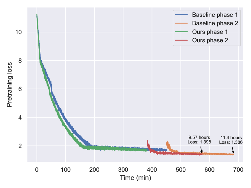
Figure A.1: Pretraining loss and time curves for BERT.

A.7 Additional Related Work

There has been significant work optimizing both transformers in particular and deep learning in general. For a comprehensive overview, see Ben-Nun & Hoefler (2019). To help guide training regimes for transformers, recent work has provided empirical recommendations on model size, batch size, and so on Li et al. (2020); Kaplan et al. (2020); Rosenfeld et al. (2020). Many of the subsequent techniques we review are complementary to our work.

Most directly relevant are other approaches specifically to accelerate transformer training. Distributed-memory techniques, such as ZeRO Rajbhandari et al. (2019), Megatron Shoeybi et al. (2019), and Mesh-TensorFlow Shazeer et al. (2018) scale training to many GPUs to accelerate it. Mesh-TensorFlow also presents a classification of operators similar to ours. Large batches have also been used to accelerate training via LAMB You et al. (2020) or NVLAMB NVIDIA AI (2019). None of these directly address the performance of a single GPU as done in this paper. DeepSpeed Microsoft (2020a), which we compare with in Section 6.3, is closest to our work, but performs all optimizations and layout selections manually.

Transformer architectures to enable improved training have also been the subject of significant recent work. ALBERT Lan et al. (2019) used a combination of weight sharing and factorized embedding layers to reduce memory requirements; however compute times are unaffected. Transformer-XL Dai et al. (2019) caches prior hidden states to learn long sequences. RevNets Gomez et al. (2017), a variant of ResNets which allow activations to be reconstructed during backpropagation, have been applied to transformers. Notably, Reformer Kitaev et al. (2020) combines reversible residual layers with locality-sensitive hashing to improve the efficiency of multi-head attention. Sparsity optimizations for attention Bahdanau et al. (2014); Luong et al. (2015); Shen et al. (2018); Parmar et al. (2018); Tay et al. (2019); Child et al. (2019); Correia et al. (2019); Sukhbaatar et al. (2019); Tay et al. (2020) reduce memory and compute requirements. We view these as orthongal to our work: the same principles of data-flow analysis can be applied to optimize for sparsity and reuse.

There has also been much work on optimizing deep learning in general. Many frameworks provide implementations of transformers or their components, such as PyTorch Paszke et al. (2019), TensorFlow Abadi et al. (2015), cuDNN Chetlur et al. (2014), and others built atop these Ott et al. (2019); Wolf et al. (2019). Optimizing frameworks can also be applied to transformers Google (2020); Frostig et al. (2018); Bradbury et al. (2018); PyTorch Team (2020); Rotem et al. (2018); Jia et al. (2019d; b; a); Chen et al. (2018); Paul G. Allen School of Computer Science & Engineering, University of Washington et al. (2017); Sivathanu et al. (2019); Mirhoseini et al. (2017); Cyphers et al. (2018); Baghdadi et al. (2019); Vasilache et al. (2018); Lethin (2017); Wei et al. (2018); Truong et al. (2016); Venkat et al. (2019); Dong et al. (2019); Elango et al. (2018). None of these frameworks provide all the optimizations or the systematic study of data movement and its impact on performance. We have specifically compared against some of the most popular production frameworks: PyTorch, TensorFlow with XLA, and cuDNN. Beyond these, TASO Jia et al. (2019a) targets similar optimizations to ours by using graph substitutions, but considers only inference and does not exhaustively explore the search space.

Other optimizations, including model parallelism Van Essen et al. (2015); Jia et al. (2019d); Gholami et al. (2018); Dean et al. (2012); Chilimbi et al. (2014); Shazeer et al. (2018); Buchlovsky et al. (2019), pipeline parallelism Chen et al. (2012); Li et al. (2018); Narayanan et al. (2019); Huang et al. (2019), microbatching Oyama et al. (2018), and recomputation for memory reduction Chen et al. (2016); Jain et al. (2020) are all also applicable. Communication can also be a major bottleneck for training transformers, due to the large model size Shoeybi et al. (2019); Shazeer et al. (2018). Frameworks for inference, including TensorRT NVIDIA (2020b), Caffe2 Facebook (2020), and the ONNX Runtime Microsoft (2020), all help to enable a suite of optimizations primarily applicable during inference. Pruning Shazeer (2019); Voita et al. (2019) and distillation Sanh et al. (2019) has also been used to accelerate inference.

Neural architecture-specific optimizations have a long history outside of transformers, and have primarily targeted CNNs Krizhevsky et al. (2012); Coates et al. (2013); Goyal et al. (2017); Akiba et al. (2017); You et al. (2018); Mikami et al. (2018); Ying et al. (2018); Dryden et al. (2019a; b). Notably, Li et al. (2016) optimized data layouts for convolution.

In general, data movement reduction is a core component of high-level optimization Unat et al. (2017). Optimizing compilers, most notably components that specialize in polyhedral programs Grosser et al. (2012); Bondhugula et al. (2008), apply loop transformations (e.g., tiling, skewing) that belong to the class of data movement optimization. Other white-box approaches for separation of program definition from data optimization passes include Halide Ragan-Kelley et al. (2013), JAX Frostig et al. (2018); Bradbury et al. (2018), Legion Bauer et al. (2012), Lift Steuwer et al. (2017), and MLIR Lattner et al. (2020). The data-centric approach proposed here enables user-extensible coarse- and fine-grained data movement optimization via the flat (yet parametric) dataflow graph representation. This allows us to perform and tune complex data layout and fusion transformations that span multiple granularity levels, surpassing the optimization capabilities of the aforementioned tools and achieving state-of-the-art performance.

References

- Abadi et al. (2015) Abadi, M., Agarwal, A., Barham, P., Brevdo, E., Chen, Z., Citro, C., Corrado, G. S., Davis, A., Dean, J., Devin, M., Ghemawat, S., Goodfellow, I., Harp, A., Irving, G., Isard, M., Jia, Y., Jozefowicz, R., Kaiser, L., Kudlur, M., Levenberg, J., Mané, D., Monga, R., Moore, S., Murray, D., Olah, C., Schuster, M., Shlens, J., Steiner, B., Sutskever, I., Talwar, K., Tucker, P., Vanhoucke, V., Vasudevan, V., Viégas, F., Vinyals, O., Warden, P., Wattenberg, M., Wicke, M., Yu, Y., and Zheng, X. TensorFlow: Large-scale machine learning on heterogeneous systems, 2015. URL https://www.tensorflow.org/.
- Akiba et al. (2017) Akiba, T., Suzuki, S., and Fukuda, K. Extremely large minibatch SGD: Training ResNet-50 on ImageNet in 15 minutes. In NeurIPS 2017 Workshop: Deep Learning at Supercomputer Scale, 2017.
- Ba et al. (2016) Ba, J. L., Kiros, J. R., and Hinton, G. E. Layer normalization. arXiv preprint arXiv:1607.06450, 2016.
- Baghdadi et al. (2019) Baghdadi, R., Debbagh, A. N., Abdous, K., Zohra, B. F., Renda, A., Frankle, J. E., Carbin, M., and Amarasinghe, S. TIRAMISU: A polyhedral compiler for dense and sparse deep learning. In Workshop on Systems for ML at NeurIPS, 2019.
- Bahdanau et al. (2014) Bahdanau, D., Cho, K., and Bengio, Y. Neural machine translation by jointly learning to align and translate. In Proceedings of the Third International Conference on Learning Representations (ICLR), 2014.
- Bauer et al. (2012) Bauer, M., Treichler, S., Slaughter, E., and Aiken, A. Legion: Expressing locality and independence with logical regions. In Proceedings of the International Conference on High Performance Computing, Networking, Storage and Analysis (SC), 2012.
- Bello et al. (2019) Bello, I., Zoph, B., Vaswani, A., Shlens, J., and Le, Q. V. Attention augmented convolutional networks. In Proceedings of the IEEE International Conference on Computer Vision (CVPR), 2019.
- Ben-Nun & Hoefler (2019) Ben-Nun, T. and Hoefler, T. Demystifying parallel and distributed deep learning: An in-depth concurrency analysis. ACM Comput. Surv., 52(4), 2019.
- Ben-Nun et al. (2019) Ben-Nun, T., de Fine Licht, J., Ziogas, A. N., Schneider, T., and Hoefler, T. Stateful dataflow multigraphs: A data-centric model for performance portability on heterogeneous architectures. In Proceedings of the International Conference for High Performance Computing, Networking, Storage and Analysis (SC), 2019.
- Bondhugula et al. (2008) Bondhugula, U., Baskaran, M., Krishnamoorthy, S., Ramanujam, J., Rountev, A., and Sadayappan, P. Automatic transformations for communication-minimized parallelization and locality optimization in the polyhedral model. In International Conference on Compiler Construction (ETAPS CC), 2008.
- Bradbury et al. (2018) Bradbury, J., Frostig, R., Hawkins, P., Johnson, M. J., Leary, C., Maclaurin, D., and Wanderman-Milne, S. JAX: composable transformations of Python+NumPy programs, 2018. URL http://github.com/google/jax.
- Bronstein et al. (2017) Bronstein, M. M., Bruna, J., LeCun, Y., Szlam, A., and Vandergheynst, P. Geometric deep learning: going beyond Euclidean data. IEEE Signal Processing Magazine, 34(4), 2017.
- Brown et al. (2020) Brown, T. B., Mann, B., Ryder, N., Subbiah, M., Kaplan, J., Dhariwal, P., Neelakantan, A., Shyam, P., Sastry, G., Askell, A., et al. Language models are few-shot learners. arXiv preprint arXiv:2005.14165, 2020.
- Buchlovsky et al. (2019) Buchlovsky, P., Budden, D., Grewe, D., Jones, C., Aslanides, J., Besse, F., Brock, A., Clark, A., Colmenarejo, S. G., Pope, A., et al. TF-Replicator: Distributed machine learning for researchers. arXiv preprint arXiv:1902.00465, 2019.
- Cerebras (2020) Cerebras. Cerebras CS-1 Product Overview, 2020. URL https://www.cerebras.net/product.
- Chellapilla et al. (2006) Chellapilla, K., Puri, S., and Simard, P. High performance convolutional neural networks for document processing. In Tenth International Workshop on Frontiers in Handwriting Recognition, 2006.
- Chen et al. (2016) Chen, T., Xu, B., Zhang, C., and Guestrin, C. Training deep nets with sublinear memory cost. arXiv preprint arXiv:1604.06174, 2016.
- Chen et al. (2018) Chen, T., Moreau, T., Jiang, Z., Zheng, L., Yan, E., Shen, H., Cowan, M., Wang, L., Hu, Y., Ceze, L., Guestrin, C., and Krishnamurthy, A. TVM: An end-to-end optimization stack for deep learning. In 13th USENIX Symposium on Operating Systems Design and Implementation (OSDI), 2018.
- Chen et al. (2012) Chen, X., Eversole, A., Li, G., Yu, D., and Seide, F. Pipelined back-propagation for context-dependent deep neural networks. In Thirteenth Annual Conference of the International Speech Communication Association (INTERSPEECH), 2012.
- Chetlur et al. (2014) Chetlur, S., Woolley, C., Vandermersch, P., Cohen, J., Tran, J., Catanzaro, B., and Shelhamer, E. cuDNN: Efficient primitives for deep learning. arXiv preprint arXiv:1410.0759, 2014.
- Child et al. (2019) Child, R., Gray, S., Radford, A., and Sutskever, I. Generating long sequences with sparse transformers. arXiv preprint arXiv:1904.10509, 2019.
- Chilimbi et al. (2014) Chilimbi, T., Suzue, Y., Apacible, J., and Kalyanaraman, K. Project Adam: Building an efficient and scalable deep learning training system. In 11th USENIX Symposium on Operating Systems Design and Implementation (OSDI), 2014.
- Cho et al. (2014) Cho, K., Van Merriënboer, B., Gulcehre, C., Bahdanau, D., Bougares, F., Schwenk, H., and Bengio, Y. Learning phrase representations using RNN encoder-decoder for statistical machine translation. In Proceedings of the 2014 Conference on Empirical Methods in Natural Language Processing (EMNLP), 2014.
- Coates et al. (2013) Coates, A., Huval, B., Wang, T., Wu, D., Catanzaro, B., and Andrew, N. Deep learning with COTS HPC systems. In International Conference on Machine Learning (ICML), 2013.
- Cordonnier et al. (2020) Cordonnier, J.-B., Loukas, A., and Jaggi, M. On the relationship between self-attention and convolutional layers. In Proceedings of the Eighth International Conference on Learning Representations (ICLR), 2020.
- Correia et al. (2019) Correia, G. M., Niculae, V., and Martins, A. F. Adaptively sparse transformers. In Proceedings of the 2019 Conference on Empirical Methods in Natural Language Processing and the 9th International Joint Conference on Natural Language Processing (EMNLP-IJCNLP), 2019.
- Cyphers et al. (2018) Cyphers, S., Bansal, A. K., Bhiwandiwalla, A., Bobba, J., Brookhart, M., Chakraborty, A., Constable, W., Convey, C., Cook, L., Kanawi, O., et al. Intel nGraph: An intermediate representation, compiler, and executor for deep learning. arXiv preprint arXiv:1801.08058, 2018.
- Dai et al. (2019) Dai, Z., Yang, Z., Yang, Y., Carbonell, J., Le, Q. V., and Salakhutdinov, R. Transformer-XL: Attentive language models beyond a fixed-length context. In Proceedings of the 57th Annual Meeting of the Association for Computational Linguistics (ACL), 2019.
- Dean et al. (2012) Dean, J., Corrado, G., Monga, R., Chen, K., Devin, M., Mao, M., Ranzato, M., Senior, A., Tucker, P., Yang, K., et al. Large scale distributed deep networks. In Advances in neural information processing systems (NeurIPS), 2012.
- Devlin et al. (2019) Devlin, J., Chang, M.-W., Lee, K., and Toutanova, K. BERT: Pre-training of deep bidirectional transformers for language understanding. In Proceedings of the 2019 Conference of the North American Chapter of the Association for Computational Linguistics (NAACL), 2019.
- Dong et al. (2019) Dong, X., Liu, L., Zhao, P., Li, G., Li, J., Wang, X., and Feng, X. Acorns: A framework for accelerating deep neural networks with input sparsity. In 2019 28th International Conference on Parallel Architectures and Compilation Techniques (PACT), 2019.
- Dosovitskiy et al. (2020) Dosovitskiy, A., Beyer, L., Kolesnikov, A., Weissenborn, D., Zhai, X., Unterthiner, T., Dehghani, M., Minderer, M., Heigold, G., Gelly, S., et al. An image is worth 16x16 words: Transformers for image recognition at scale. arXiv preprint arXiv:2010.11929, 2020.
- Dryden et al. (2019a) Dryden, N., Maruyama, N., Benson, T., Moon, T., Snir, M., and Van Essen, B. Improving strong-scaling of CNN training by exploiting finer-grained parallelism. In 2019 IEEE International Parallel and Distributed Processing Symposium (IPDPS), 2019a.
- Dryden et al. (2019b) Dryden, N., Maruyama, N., Moon, T., Benson, T., Snir, M., and Van Essen, B. Channel and filter parallelism for large-scale CNN training. In Proceedings of the International Conference for High Performance Computing, Networking, Storage and Analysis (SC), 2019b.
- Elango et al. (2018) Elango, V., Rubin, N., Ravishankar, M., Sandanagobalane, H., and Grover, V. Diesel: DSL for linear algebra and neural net computations on GPUs. In Proceedings of the 2nd ACM SIGPLAN International Workshop on Machine Learning and Programming Languages, 2018.
- Facebook (2020) Facebook. Caffe2, 2020. URL https://caffe2.ai/.
- Frostig et al. (2018) Frostig, R., Johnson, M. J., and Leary, C. Compiling machine learning programs via high-level tracing. Systems for Machine Learning, 2018.
- Fuhrer et al. (2018) Fuhrer, O., Chadha, T., Hoefler, T., Kwasniewski, G., Lapillonne, X., Leutwyler, D., Lüthi, D., Osuna, C., Schär, C., Schulthess, T. C., et al. Near-global climate simulation at 1 km resolution: establishing a performance baseline on 4888 GPUs with COSMO 5.0. Geoscientific Model Development, 11(4), 2018.
- Gholami et al. (2018) Gholami, A., Azad, A., Jin, P., Keutzer, K., and Buluc, A. Integrated model, batch, and domain parallelism in training neural networks. In Proceedings of the 30th on Symposium on Parallelism in Algorithms and Architectures (SPAA), 2018.
- Gomez et al. (2017) Gomez, A. N., Ren, M., Urtasun, R., and Grosse, R. B. The reversible residual network: Backpropagation without storing activations. In Advances in neural information processing systems (NeurIPS), 2017.
- Goodfellow et al. (2016) Goodfellow, I., Bengio, Y., and Courville, A. Deep Learning. MIT Press, 2016. http://www.deeplearningbook.org.
- Google (2020) Google. XLA: Optimizing compiler for machine learning, 2020. URL https://www.tensorflow.org/xla.
- Goyal et al. (2017) Goyal, P., Dollár, P., Girshick, R., Noordhuis, P., Wesolowski, L., Kyrola, A., Tulloch, A., Jia, Y., and He, K. Accurate, large minibatch SGD: training ImageNet in 1 hour. arXiv preprint arXiv:1706.02677, 2017.
- Graves (2012) Graves, A. Sequence transduction with recurrent neural networks. International Conference on Machine Learning (ICML) Workshop on Representation Learning, 2012.
- Grosser et al. (2012) Grosser, T., Größlinger, A., and Lengauer, C. Polly - performing polyhedral optimizations on a low-level intermediate representation. Parallel Processing Letters, 22(4), 2012.
- He et al. (2016) He, K., Zhang, X., Ren, S., and Sun, J. Deep residual learning for image recognition. In Proceedings of the IEEE International Conference on Computer Vision (CVPR), 2016.
- Hochreiter & Schmidhuber (1997) Hochreiter, S. and Schmidhuber, J. Long short-term memory. Neural Computation, 9(8), 1997.
- Huang et al. (2019) Huang, Y., Cheng, Y., Bapna, A., Firat, O., Chen, D., Chen, M., Lee, H., Ngiam, J., Le, Q. V., Wu, Y., et al. GPipe: Efficient training of giant neural networks using pipeline parallelism. In Advances in Neural Information Processing Systems (NeurIPS), 2019.
- Jain et al. (2020) Jain, P., Jain, A., Nrusimha, A., Gholami, A., Abbeel, P., Keutzer, K., Stoica, I., and Gonzalez, J. E. Checkmate: Breaking the memory wall with optimal tensor rematerialization. In Proceedings of the Third Conference on Machine Learning and Systems (MLSys), 2020.
- Jia et al. (2019a) Jia, Z., Padon, O., Thomas, J., Warszawski, T., Zaharia, M., and Aiken, A. TASO: optimizing deep learning computation with automatic generation of graph substitutions. In Proceedings of the 27th ACM Symposium on Operating Systems Principles (SOSP), 2019a.
- Jia et al. (2019b) Jia, Z., Thomas, J., Warszawski, T., Gao, M., Zaharia, M., and Aiken, A. Optimizing DNN computation with relaxed graph substitutions. In Proceedings of the 2nd Conference on Systems and Machine Learning (SysML), 2019b.
- Jia et al. (2019c) Jia, Z., Tillman, B., Maggioni, M., and Scarpazza, D. P. Dissecting the Graphcore IPU architecture via microbenchmarking, 2019c.
- Jia et al. (2019d) Jia, Z., Zaharia, M., and Aiken, A. Beyond data and model parallelism for deep neural networks. In Proceedings of the 2nd Conference on Systems and Machine Learning (SysML), 2019d.
- Jia-Wei & Kung (1981) Jia-Wei, H. and Kung, H.-T. I/O complexity: The red-blue pebble game. In Proceedings of the thirteenth annual ACM symposium on Theory of computing, 1981.
- Jouppi et al. (2017) Jouppi, N. P., Young, C., Patil, N., Patterson, D., Agrawal, G., Bajwa, R., Bates, S., Bhatia, S., Boden, N., Borchers, A., et al. In-datacenter performance analysis of a tensor processing unit. In Proceedings of the 44th Annual International Symposium on Computer Architecture (ISCA), 2017.
- Kalchbrenner & Blunsom (2013) Kalchbrenner, N. and Blunsom, P. Recurrent continuous translation models. In Proceedings of the 2013 Conference on Empirical Methods in Natural Language Processing (EMNLP), 2013.
- Kaplan et al. (2020) Kaplan, J., McCandlish, S., Henighan, T., Brown, T. B., Chess, B., Child, R., Gray, S., Radford, A., Wu, J., and Amodei, D. Scaling laws for neural language models. arXiv preprint arXiv:2001.08361, 2020.
- Keskar et al. (2019) Keskar, N. S., McCann, B., Varshney, L. R., Xiong, C., and Socher, R. CTRL: A conditional transformer language model for controllable generation. arXiv preprint arXiv:1909.05858, 2019.
- Kitaev et al. (2020) Kitaev, N., Kaiser, Ł., and Levskaya, A. Reformer: The efficient transformer. In Proceedings of the Eighth International Conference on Learning Representations (ICLR), 2020.
- Krizhevsky et al. (2012) Krizhevsky, A., Sutskever, I., and Hinton, G. E. ImageNet classification with deep convolutional neural networks. In Advances in Neural Information Processing Systems (NeurIPS), 2012.
- Lample & Charton (2019) Lample, G. and Charton, F. Deep learning for symbolic mathematics. arXiv preprint arXiv:1912.01412, 2019.
- Lan et al. (2019) Lan, Z., Chen, M., Goodman, S., Gimpel, K., Sharma, P., and Soricut, R. ALBERT: A lite BERT for self-supervised learning of language representations. In Proceedings of the Seventh International Conference on Learning Representations (ICLR), 2019.
- Lattner et al. (2020) Lattner, C., Pienaar, J., Amini, M., Bondhugula, U., Riddle, R., Cohen, A., Shpeisman, T., Davis, A., Vasilache, N., and Zinenko, O. MLIR: A compiler infrastructure for the end of moore’s law. arXiv preprint arXiv:2002.11054, 2020.
- Lavin & Gray (2016) Lavin, A. and Gray, S. Fast algorithms for convolutional neural networks. In Proceedings of the IEEE Conference on Computer Vision and Pattern Recognition (CVPR), 2016.
- Lethin (2017) Lethin, R. Polyhedral optimization of tensorflow computation graphs. In Sixth Workshop on Extreme-scale Programming Tools (ESPT), 2017.
- Li et al. (2016) Li, C., Yang, Y., Feng, M., Chakradhar, S., and Zhou, H. Optimizing memory efficiency for deep convolutional neural networks on GPUs. In Proceedings of the International Conference for High Performance Computing, Networking, Storage and Analysis (SC), 2016.
- Li et al. (2018) Li, Y., Yu, M., Li, S., Avestimehr, S., Kim, N. S., and Schwing, A. Pipe-SGD: A decentralized pipelined SGD framework for distributed deep net training. In Advances in Neural Information Processing Systems (NeurIPS), 2018.
- Li et al. (2020) Li, Z., Wallace, E., Shen, S., Lin, K., Keutzer, K., Klein, D., and Gonzalez, J. E. Train large, then compress: Rethinking model size for efficient training and inference of transformers. arXiv preprint arXiv:2002.11794, 2020.
- Liu et al. (2019) Liu, Y., Ott, M., Goyal, N., Du, J., Joshi, M., Chen, D., Levy, O., Lewis, M., Zettlemoyer, L., and Stoyanov, V. RoBERTa: A robustly optimized BERT pretraining approach. arXiv preprint arXiv:1907.11692, 2019.
- Livermore Computing Center (2020) Livermore Computing Center. Lassen, 2020. URL https://hpc.llnl.gov/hardware/platforms/lassen.
- Luong et al. (2015) Luong, M.-T., Pham, H., and Manning, C. D. Effective approaches to attention-based neural machine translation. In Proceedings of the 2015 Conference on Empirical Methods in Natural Language Processing (EMNLP), 2015.
- Mathieu et al. (2013) Mathieu, M., Henaff, M., and LeCun, Y. Fast training of convolutional networks through FFTs. arXiv preprint arXiv:1312.5851, 2013.
- Maziarka et al. (2020) Maziarka, Ł., Danel, T., Mucha, S., Rataj, K., Tabor, J., and Jastrzębski, S. Molecule attention transformer. arXiv preprint arXiv:2002.08264, 2020.
- Micikevicius et al. (2018) Micikevicius, P., Narang, S., Alben, J., Diamos, G., Elsen, E., Garcia, D., Ginsburg, B., Houston, M., Kuchaiev, O., Venkatesh, G., et al. Mixed precision training. In Proceedings of the Sixth International Conference on Learning Representations (ICLR), 2018.
- Microsoft (2020a) Microsoft. DeepSpeed, 2020a. URL deepspeed.ai.
- Microsoft (2020b) Microsoft. Turing-NLG: A 17-billion-parameter language model by Microsoft, 2020b. URL https://www.microsoft.com/en-us/research/blog/turing-nlg-a-17-billion-parameter-language-model-by-microsoft/.
- Microsoft (2020c) Microsoft. ZeRO & DeepSpeed: New system optimizations enable training models with over 100 billion parameters, 2020c. URL https://www.microsoft.com/en-us/research/blog/zero-deepspeed-new-system-optimizations-enable-training-models-with-over-100-billion-parameters/.
- Microsoft (2020) Microsoft. ONNX Runtime, 2020. URL https://microsoft.github.io/onnxruntime/.
- Mikami et al. (2018) Mikami, H., Suganuma, H., U-chupala, P., Tanaka, Y., and Kageyama, Y. Massively distributed SGD: ImageNet/ResNet-50 training in a flash. arXiv preprint arXiv:1811.05233, 2018.
- Mikolov et al. (2013a) Mikolov, T., Chen, K., Corrado, G., and Dean, J. Efficient estimation of word representations in vector space. arXiv preprint arXiv:1301.3781, 2013a.
- Mikolov et al. (2013b) Mikolov, T., Sutskever, I., Chen, K., Corrado, G. S., and Dean, J. Distributed representations of words and phrases and their compositionality. In Advances in neural information processing systems (NeurIPS), 2013b.
- Mikolov et al. (2013c) Mikolov, T., Yih, W.-t., and Zweig, G. Linguistic regularities in continuous space word representations. In Proceedings of the 2013 Conference of the North American Chapter of the Association for Computational Linguistics (NAACL), 2013c.
- Mirhoseini et al. (2017) Mirhoseini, A., Pham, H., Le, Q. V., Steiner, B., Larsen, R., Zhou, Y., Kumar, N., Norouzi, M., Bengio, S., and Dean, J. Device placement optimization with reinforcement learning. In Proceedings of the 34th International Conference on Machine Learning, 2017.
- Narayanan et al. (2019) Narayanan, D., Harlap, A., Phanishayee, A., Seshadri, V., Devanur, N. R., Ganger, G. R., Gibbons, P. B., and Zaharia, M. PipeDream: generalized pipeline parallelism for dnn training. In Proceedings of the 27th ACM Symposium on Operating Systems Principles (SOSP), 2019.
- Nvidia (2020a) Nvidia. Apex (A PyTorch Extension), 2020a. URL https://nvidia.github.io/apex/.
- Nvidia (2020b) Nvidia. CUTLASS: CUDA templates for linear algebra subroutines, 2020b. URL https://github.com/NVIDIA/cutlass.
- NVIDIA (2020a) NVIDIA. NVIDIA deep learning examples, 2020a. URL https://github.com/NVIDIA/DeepLearningExamples.
- NVIDIA (2020b) NVIDIA. NVIDIA TensorRT, 2020b. URL https://developer.nvidia.com/tensorrt.
- Nvidia (2020) Nvidia. TensorFloat-32 in the A100 GPU Accelerates AI Training, HPC up to 20x, 2020. URL https://blogs.nvidia.com/blog/2020/05/14/tensorfloat-32-precision-format.
- NVIDIA AI (2019) NVIDIA AI. A guide to optimizer implementation for BERT at scale, 2019. URL https://medium.com/nvidia-ai/a-guide-to-optimizer-implementation-for-bert-at-scale-8338cc7f45fd.
- OpenAI (2018) OpenAI. AI and compute, 2018. URL https://openai.com/blog/ai-and-compute/.
- OpenAI (2019) OpenAI. Microsoft invests in and partners with OpenAI to support us building beneficial AGI, 2019. URL https://openai.com/blog/microsoft/.
- Ott et al. (2019) Ott, M., Edunov, S., Baevski, A., Fan, A., Gross, S., Ng, N., Grangier, D., and Auli, M. fairseq: A fast, extensible toolkit for sequence modeling. In Proceedings of NAACL-HLT 2019: Demonstrations, 2019.
- Oyama et al. (2018) Oyama, Y., Ben-Nun, T., Hoefler, T., and Matsuoka, S. Accelerating deep learning frameworks with micro-batches. In 2018 IEEE International Conference on Cluster Computing (CLUSTER), 2018.
- Parisotto et al. (2019) Parisotto, E., Song, H. F., Rae, J. W., Pascanu, R., Gulcehre, C., Jayakumar, S. M., Jaderberg, M., Kaufman, R. L., Clark, A., Noury, S., et al. Stabilizing transformers for reinforcement learning. arXiv preprint arXiv:1910.06764, 2019.
- Parmar et al. (2018) Parmar, N., Vaswani, A., Uszkoreit, J., Kaiser, Ł., Shazeer, N., Ku, A., and Tran, D. Image transformer. In Proceedings of the 35th International Conference on Machine Learning (ICML), 2018.
- Parmar et al. (2019) Parmar, N., Ramachandran, P., Vaswani, A., Bello, I., Levskaya, A., and Shlens, J. Stand-alone self-attention in vision models. In Advances in Neural Information Processing Systems (NeurIPS), 2019.
- Paszke et al. (2019) Paszke, A., Gross, S., Massa, F., Lerer, A., Bradbury, J., Chanan, G., Killeen, T., Lin, Z., Gimelshein, N., Antiga, L., et al. PyTorch: An imperative style, high-performance deep learning library. In Advances in Neural Information Processing Systems (NeurIPS), 2019.
- Paul G. Allen School of Computer Science & Engineering, University of Washington et al. (2017) Paul G. Allen School of Computer Science & Engineering, University of Washington, Amazon Web Service AI team, and DMLC open-source community. NNVM compiler: Open compiler for AI frameworks, 2017. URL https://tvm.apache.org/2017/10/06/nnvm-compiler-announcement.
- PyTorch Team (2020) PyTorch Team. TorchScript, 2020. URL https://pytorch.org/docs/stable/jit.html.
- Radford et al. (2018) Radford, A., Narasimhan, K., Salimans, T., and Sutskever, I. Improving language understanding by generative pre-training, 2018. URL https://s3-us-west-2.amazonaws.com/openai-assets/research-covers/language-unsupervised/language_understanding_paper.pdf.
- Radford et al. (2019) Radford, A., Wu, J., Child, R., Luan, D., Amodei, D., and Sutskever, I. Language models are unsupervised multitask learners, 2019. URL https://openai.com/blog/better-language-models/.
- Raffel et al. (2019) Raffel, C., Shazeer, N., Roberts, A., Lee, K., Narang, S., Matena, M., Zhou, Y., Li, W., and Liu, P. J. Exploring the limits of transfer learning with a unified text-to-text transformer. arXiv preprint arXiv:1910.10683, 2019.
- Ragan-Kelley et al. (2013) Ragan-Kelley, J., Barnes, C., Adams, A., Paris, S., Durand, F., and Amarasinghe, S. Halide: A language and compiler for optimizing parallelism, locality, and recomputation in image processing pipelines. ACM SIGPLAN Notices, 48(6), 2013.
- Rajbhandari et al. (2019) Rajbhandari, S., Rasley, J., Ruwase, O., and He, Y. ZeRO: Memory optimization towards training a trillion parameter models. arXiv preprint arXiv:1910.02054, 2019.
- Rajpurkar et al. (2018) Rajpurkar, P., Jia, R., and Liang, P. Know what you don’t know: Unanswerable questions for SQuAD. In Proceedings of the 56th Annual Meeting of the Association for Computational Linguistics (ACL), 2018.
- Rosenfeld et al. (2020) Rosenfeld, J. S., Rosenfeld, A., Belinkov, Y., and Shavit, N. A constructive prediction of the generalization error across scales. In Proceedings of the Eighth International Conference on Learning Representations (ICLR), 2020.
- Rotem et al. (2018) Rotem, N., Fix, J., Abdulrasool, S., Catron, G., Deng, S., Dzhabarov, R., Gibson, N., Hegeman, J., Lele, M., Levenstein, R., et al. Glow: Graph lowering compiler techniques for neural networks. arXiv preprint arXiv:1805.00907, 2018.
- Rumelhart et al. (1986) Rumelhart, D. E., Hinton, G. E., and Williams, R. J. Learning representations by back-propagating errors. Nature, 323(6088), 1986.
- Sabour et al. (2017) Sabour, S., Frosst, N., and Hinton, G. E. Dynamic routing between capsules. In Advances in neural information processing systems (NeurIPS), 2017.
- Sanh et al. (2019) Sanh, V., Debut, L., Chaumond, J., and Wolf, T. DistilBERT, a distilled version of BERT: smaller, faster, cheaper and lighter. In Fifth Workshop on Energy Efficient Machine Learning and Cognitive Computing at NeurIPS 2019, 2019.
- Shazeer (2019) Shazeer, N. Fast transformer decoding: One write-head is all you need. arXiv preprint arXiv:1911.02150, 2019.
- Shazeer et al. (2018) Shazeer, N., Cheng, Y., Parmar, N., Tran, D., Vaswani, A., Koanantakool, P., Hawkins, P., Lee, H., Hong, M., Young, C., et al. Mesh-TensorFlow: Deep learning for supercomputers. In Advances in Neural Information Processing Systems (NeurIPS), 2018.
- Shen et al. (2018) Shen, T., Zhou, T., Long, G., Jiang, J., and Zhang, C. Bi-directional block self-attention for fast and memory-efficient sequence modeling. In Proceedings of the Sixth International Conference on Learning Representations (ICLR), 2018.
- Shoeybi et al. (2019) Shoeybi, M., Patwary, M., Puri, R., LeGresley, P., Casper, J., and Catanzaro, B. Megatron-LM: Training multi-billion parameter language models using GPU model parallelism. arXiv preprint arXiv:1909.08053, 2019.
- Sivathanu et al. (2019) Sivathanu, M., Chugh, T., Singapuram, S. S., and Zhou, L. Astra: Exploiting predictability to optimize deep learning. In Proceedings of the Twenty-Fourth International Conference on Architectural Support for Programming Languages and Operating Systems (ASPLOS), 2019.
- Srivastava et al. (2014) Srivastava, N., Hinton, G., Krizhevsky, A., Sutskever, I., and Salakhutdinov, R. Dropout: a simple way to prevent neural networks from overfitting. Journal of machine learning research (JMLR), 15(1), 2014.
- Steuwer et al. (2017) Steuwer, M., Remmelg, T., and Dubach, C. Lift: A functional data-parallel ir for high-performance gpu code generation. In Proceedings of the 2017 International Symposium on Code Generation and Optimization (CGO), 2017.
- Strubell et al. (2019) Strubell, E., Ganesh, A., and McCallum, A. Energy and policy considerations for deep learning in NLP. In Proceedings of the 57th Annual Meeting of the Association for Computational Linguistics (ACL), 2019.
- Sukhbaatar et al. (2019) Sukhbaatar, S., Grave, E., Bojanowski, P., and Joulin, A. Adaptive attention span in transformers. In Proceedings of the 57th Annual Meeting of the Association for Computational Linguistics (ACL), 2019.
- Sutskever et al. (2014) Sutskever, I., Vinyals, O., and Le, Q. V. Sequence to sequence learning with neural networks. In Advances in neural information processing systems (NeurIPS), 2014.
- Tay et al. (2019) Tay, Y., Wang, S., Tuan, L. A., Fu, J., Phan, M. C., Yuan, X., Rao, J., Hui, S. C., and Zhang, A. Simple and effective curriculum pointer-generator networks for reading comprehension over long narratives. In Proceedings of the 57th Annual Meeting of the Association for Computational Linguistics (ACL), 2019.
- Tay et al. (2020) Tay, Y., Bahri, D., Yang, L., Metzler, D., and Juan, D.-C. Sparse sinkhorn attention. arXiv preprint arXiv:2002.11296, 2020.
- Truong et al. (2016) Truong, L., Barik, R., Totoni, E., Liu, H., Markley, C., Fox, A., and Shpeisman, T. Latte: A language, compiler, and runtime for elegant and efficient deep neural networks. In Proceedings of the 37th ACM SIGPLAN Conference on Programming Language Design and Implementation (PLDI), 2016.
- Unat et al. (2017) Unat, D., Dubey, A., Hoefler, T., Shalf, J., Abraham, M., Bianco, M., Chamberlain, B. L., Cledat, R., Edwards, H. C., Finkel, H., Fuerlinger, K., Hannig, F., Jeannot, E., Kamil, A., Keasler, J., Kelly, P. H. J., Leung, V., Ltaief, H., Maruyama, N., Newburn, C. J., , and Pericas, M. Trends in Data Locality Abstractions for HPC Systems. IEEE Transactions on Parallel and Distributed Systems (TPDS), 28(10), 2017.
- Van Essen et al. (2015) Van Essen, B., Kim, H., Pearce, R., Boakye, K., and Chen, B. LBANN: Livermore big artificial neural network HPC toolkit. In Proceedings of the Workshop on Machine Learning in High-Performance Computing Environments (MLHPC), 2015.
- Vasilache et al. (2018) Vasilache, N., Zinenko, O., Theodoridis, T., Goyal, P., DeVito, Z., Moses, W. S., Verdoolaege, S., Adams, A., and Cohen, A. Tensor comprehensions: Framework-agnostic high-performance machine learning abstractions. arXiv preprint arXiv:1802.04730, 2018.
- Vaswani et al. (2017) Vaswani, A., Shazeer, N., Parmar, N., Uszkoreit, J., Jones, L., Gomez, A. N., Kaiser, Ł., and Polosukhin, I. Attention is all you need. In Advances in Neural Information Processing Systems (NeurIPS), 2017.
- Venkat et al. (2019) Venkat, A., Rusira, T., Barik, R., Hall, M., and Truong, L. SWIRL: High-performance many-core CPU code generation for deep neural networks. The International Journal of High Performance Computing Applications, 33(6), 2019.
- Voita et al. (2019) Voita, E., Talbot, D., Moiseev, F., Sennrich, R., and Titov, I. Analyzing multi-head self-attention: Specialized heads do the heavy lifting, the rest can be pruned. In Proceedings of the 57th Annual Meeting of the Association for Computational Linguistics (ACL), 2019.
- Wang et al. (2018) Wang, A., Singh, A., Michael, J., Hill, F., Levy, O., and Bowman, S. R. GLUE: A multi-task benchmark and analysis platform for natural language understanding. In Proceedings of the 2018 EMNLP Workshop BlackboxNLP: Analyzing and Interpreting Neural Networks for NLP, 2018.
- Wang et al. (2019) Wang, A., Pruksachatkun, Y., Nangia, N., Singh, A., Michael, J., Hill, F., Levy, O., and Bowman, S. SuperGLUE: A stickier benchmark for general-purpose language understanding systems. In Advances in Neural Information Processing Systems (NeurIPS), 2019.
- Wei et al. (2018) Wei, R., Schwartz, L., and Adve, V. DLVM: A modern compiler infrastructure for deep learning systems. In Proceedings of the Sixth International Conference on Learning Representations - Workshop Track (ICLR), 2018.
- Wiggers (2020) Wiggers, K. OpenAI’s massive GPT-3 model is impressive, but size isn’t everything, 2020. URL https://venturebeat.com/2020/06/01/ai-machine-learning-openai-gpt-3-size-isnt-everything/.
- Wolf et al. (2019) Wolf, T., Debut, L., Sanh, V., Chaumond, J., Delangue, C., Moi, A., Cistac, P., Rault, T., Louf, R., Funtowicz, M., and Brew, J. HuggingFace’s transformers: State-of-the-art natural language processing. arXiv preprint arXiv:1910.03771, 2019.
- Yang et al. (2019) Yang, Z., Dai, Z., Yang, Y., Carbonell, J., Salakhutdinov, R. R., and Le, Q. V. XLNet: Generalized autoregressive pretraining for language understanding. In Advances in Neural Information Processing Systems (NeurIPS), 2019.
- Yeh et al. (2019) Yeh, C.-F., Mahadeokar, J., Kalgaonkar, K., Wang, Y., Le, D., Jain, M., Schubert, K., Fuegen, C., and Seltzer, M. L. Transformer-transducer: End-to-end speech recognition with self-attention. arXiv preprint arXiv:1910.12977, 2019.
- Ying et al. (2018) Ying, C., Kumar, S., Chen, D., Wang, T., and Cheng, Y. Image classification at supercomputer scale. In NeurIPS Systems for ML Workshop, 2018.
- You et al. (2018) You, Y., Zhang, Z., Hsieh, C.-J., Demmel, J., and Keutzer, K. ImageNet training in minutes. In Proceedings of the 47th International Conference on Parallel Processing (ICPP), 2018.
- You et al. (2020) You, Y., Li, J., Reddi, S., Hseu, J., Kumar, S., Bhojanapalli, S., Song, X., Demmel, J., Keutzer, K., and Hsieh, C.-J. Large batch optimization for deep learning: Training BERT in 76 minutes. In Proceedings of the Eighth International Conference on Learning Representations (ICLR), 2020.
- Ziogas et al. (2019) Ziogas, A. N., Ben-Nun, T., Fernández, G. I., Schneider, T., Luisier, M., and Hoefler, T. A data-centric approach to extreme-scale ab initio dissipative quantum transport simulations. In Proceedings of the International Conference for High Performance Computing, Networking, Storage and Analysis (SC), 2019.