Preconditioning Markov Chain Monte Carlo Method for Geomechanical Subsidence using multiscale method and machine learning technique

Abstract

In this paper, we consider the numerical solution of the poroelasticity problem with stochastic properties. We present a Two-stage Markov Chain Monte Carlo method for geomechanical subsidence. In this work, we study two techniques of preconditioning: (MS) multiscale method for model order reduction and (ML) machine learning technique. The purpose of preconditioning is the fast sampling, where a new proposal is first testes by a cheap multiscale solver or using fast prediction of the neural network and the full fine grid computations will be conducted only if the proposal passes the first step. To construct a reduced order model, we use the Generalized Multiscale Finite Element Method and present construction of the multiscale basis functions for pressure and displacements in stochastic fields. In order to construct a machine learning based preconditioning, we generate a dataset using a multiscale solver and use it to train neural networks. The Karhunen-Loéve expansion is used to represent the realization of the stochastic field. Numerical results are presented for two- and three-dimensional model examples.

1 Introduction

Modelling geomechanical problems has important implications on the understanding of many of the physical processes. For example, in areas such as environmental engineering with modelling permafrost compaction and subsidence [26], and the oil and gas industry for reservoir geomechanics to increase production and overall reservoir life [29, 40]. There are many challenges in simulating these problems. One challenging being the length scales involved. There is a high variability in material parameters such as permeability and porosity for flow and Young’s modulus in the case of mechanical properties. Further compounding the problem is lack of knowledge of these parameters due to subsurface depth. This uncertainty may arise from under resolution from seismic data or, in the case of resistivity measurements with electromagnetic sensors, unclear physical matching of properties to data.

As noted, the computational challenge is often two fold. First, heterogeneity of subsurface properties need to be accurately accounted for in the geomechanical model. In turn, this requires high resolution with adding many degrees of freedom that can be computationally expensive. Second is the uncertainty in the subsurface properties such as permeability and elastic parameters. However, in today’s “Big-Data” world, often a plethora of information is available to help characterize the subsurface. For example, in reservoir engineering there is extensive logs on production data such as oil-cut of produced wells. In addition, other metrics such as bottom hole pressure and time of flight have been extensively used in the history matching literature to integrate data into the subsurface models [22, 39]. In the areas of environmental science and engineering, near-surface resistivity measurements are often available to obtain constraints on subsurface moisture content reflit.

There are various techniques to integrate data into subsurface models. The literature is quite extensive and various uncertainty quantification methodologies exist and have various advantages and disadvantages. Various data assimilations and variants are often used to integrate dynamic data information constantly into models. This is particularly useful for weather forecast modelling as well as geophysical problems. In this work, we will consider a Bayesian framework of updating a prior probability distribution with information to obtain a data-integrated posterior. It is well known that the resulting problems are high-dimensional and suffer from the curse of dimensionality. To circumvent some of this difficulty Monte-Carlo based techniques have been proposed. For example, a popular and useful technique is the Ensemble Kalman Filter (EnKF) [13] to integrate data into subsurface models. In this work, however, we consider a Markov-Chain Monte-Carlo method (MCMC) based on the classical Metropolis-Hastings sampling algorithm [8]. This is an effective tool to efficiently sample from an unknown posterior distribution that is conditioned to the data. However, the MCMC algorithms suffer from the fact that many simulations must be computed [17, 19]. This is again tied to the multiscale and high-contrast nature of the material properties as direct numerical simulations must fully resolve these scales. Moreover, the acceptance rate of proposed subsurface properties in the Metropolis-Hastings algorithm is known to be very low.

With the availability surface sensors and satellite observation data (InSAR) [23], it is now possible to better characterize the geomechanical picture of the subsurface based on this data. This has proven particularly useful in the context of monitoring large scale CO2 sequestration projects [34, 28]. There are various subsurface mechanical models that one can consider, however, in this work we will work with a poroelastic earth model. The mathematical structure of the poroelasticity models are coupled equations for pressure and displacements known as Biot models [3]. Poroelastic models of this type have been explored in the petroleum engineering literature in the context of geomechanics for some time [31, 30, 24, 25, 27]. An interesting surface observation application such as permafrost modelling would require thermal and partially saturated moisture considerations, but we leave this to future work.

As mentioned prior, the MCMC algorithm suffer from large number of simulation runs and low acceptance rates. A useful technique to expedite this procedure is preconditioning the Metropolis-Hasting algorithm in a two-stage (or multi-stage) procedure utilizing coarse-scale or upscaled models [10]. This is accomplished by using the coarser-scale simulation as a prior filtering stage in the accept-rejection procedure. There are many effective multiscale frameworks that have been developed in recent years for the poroelasticity problem [7, 32, 2, 33, 14, 35]. We will use the Generalized Multiscale Finite Element Method (GMsFEM) framework developed for poroelasticty in [4, 5], which is a generalization of the multiscale finite element method to build our course-scale models [12]. Utilizing GMsFEMs for this application has also been useful in Multi-Level MCMC for elliptic problems with high-contrast [15].

The GMsFEM has the advantage of being able to capture small scale features from the heterogeneities into coarse-grid basis functions and offline spaces, as well as having a unified computational grids for both mechanics and flow solves. The offline multiscale basis construction may proceed in both fluid and mechanics in parallel and both constructions are comparable. First a coarse-grid is generated and in each grid block a local static problem with varying boundary conditions is solved to construct the snapshot spaces. We then perform a dimension reduction of the snapshot space by solving auxiliary eigenvalue problems. Taking the corresponding smallest eigenpairs, and multiplying by a multiscale partition of unity we are able to construct our offline basis. In this greatly reduced dimension offline basis, the online solutions may be calculated for pressure and displacements for any viable boundary condition or forcing. Given a set or material properties such as permeability a set of standard MsFEM basis functions must be computed, however, utilizing the GMsFEM’s ability to handle parameters (as is used in nonlinear GMsFEM) as well as scales we are able to compute a single set of enriched basis functions for many possible realizations of physical parameters.

For further reduction of the computational time of the first stage in the two-stage MCMC method, we present a machine learning technique [36, 37]. The machine learning is used to quickly predict displacements for the estimation of the proposed fields. We generate a dataset using a multiscale solver and use it to train neural networks and learn dependencies between heterogeneous properties and displacements in each direction on the top boundary. As soon as neural networks are trained on the dataset, fast calculations can be performed as preconditioning of the MCMC method. We use a convolutional neural network and GPU training process to construct a machine learning algorithm [20, 18].

The work is organized as follows. In Section 2, we provide the mathematical background of the geomechanical subsidence problem. We introduce the Biot type model and highlight where the heterogeneity primarily occurs. In Section 3, we discuss the fine-scale and GMsFEM (coarse-scale) solution of the geomechanical problem. We utilize the nonlinear GMsFEM for poroelasticity developed in [4], whereby we are able to handle parametrization. In Section 4 we introduce the broad concepts of Bayesian uncertainty quantification. We discuss the parametrization of the randomness via the Karhunen-Loeve expansion so that when we search in the MCMC procedure the dimension of the space is reduced. We outline the single and two-stage Metropolis-Hastings algorithms used in the accept-reject procedure to sample from the “data-integrated” posterior distribution. In Section 5, we present a numerical algorithm based on two- and three-dimensional synthetic data at the surface to show the efficiency of the method as an expedited MCMC sampling method.

2 Problem Formulation

We start with the description of the general geomechanical model that we use in our simulations. We keep the discussion very general and abstract, but ultimately the idea is to have one surface boundary that has open surface boundary conditions, and a truncated in situ ground that has fixed motion and is in physical reality connected to a much larger (functionally infinite) domain.

We denote computational domain $\Omega\subset\mathbb{R}^{d},d=2,3,$ to be a bounded sufficiently smooth (Lipschitz) region. We consider linear poroelasticity problem, with random or uncertain coefficients. That we may view as parameters. We wish to find a pressure $p$ and displacements $u$ satisfying the following Biot effective stress poroelasticity law

$$\begin{split}-\mathop{\rm div}\nolimits\sigma(x,\theta,u)+\alpha\mathop{\rm grad}\nolimits p&=0,\quad x\in\Omega,\quad t>0,\\ \alpha\frac{\partial\mathop{\rm div}\nolimits u}{\partial t}+\frac{1}{M}\frac{\partial p}{\partial t}+\mathop{\rm div}\nolimits q(x,\theta,p)&=0,\quad x\in\Omega,\quad t>0,\end{split}$$ (1)

where $M$ is the Biot modulus and $\alpha$ is the Biot-Willis fluid-solid coupling coefficient. These terms are lower order derivatives, so for simplicity we will suppose that these are constants and not random. Body forces, such as gravity, are neglected without loss of generality.

Here we suppose that the stress tensor $\sigma$ and flux $q$ depend on both space $x$ and a large dimensional random parameter $\theta$

$$q(x,\theta,p)=-\frac{k(x,\theta)}{\nu}\mathop{\rm grad}\nolimits p,\quad\sigma(x,\theta,u)=2\mu(x,\theta)\varepsilon(u)+\lambda(x,\theta)\mathop{\rm div}\nolimits u\,\mathcal{I},$$

where $\varepsilon(u)=(\mathop{\rm grad}\nolimits u+\mathop{\rm grad}\nolimits u^{T})/2$, $\nu$ is the fluid viscosity, $k(x,\theta)$ is the permeability, $\mu(x,\theta)$, $\lambda(x,\theta)$ are Lamé coefficients, $\mathcal{I}$ is the identity tensor.

For Lamé coefficients $\lambda$ and $\mu$, we have following relations

$$\mu(x,\theta)=\frac{E(x,\theta)}{2(1+\eta)},\quad\lambda(x,\theta)=\frac{E(x,\theta)\eta}{(1+\eta)(1-2\eta)},$$

where $E(x,\theta)$ is the random spatially varying elastic modulus and $\eta$ is a constant Poisson’s ratio. One could choose to vary both, but for this work we consider a varying elastic modulus. Thus, the coefficients $k(x,\theta)$, $\mu(x,\theta)$ and $\lambda(x,\theta)$ may be highly variable and contain randomness or uncertainty.

We denote the initial condition for pressure

$$p=p_{0},\quad x\in\Omega,\quad t=0.$$

In general, we suppose the following Neumann and Robyn boundary conditions on each portion

$$u=0,\quad x\in\Gamma_{u},\quad\sigma\cdot n=0,\quad x\in\partial\Omega/\Gamma_{u},$$

and

$$q\cdot n=\gamma(p-p_{1}),\quad x\in\Gamma_{p},\quad q\cdot n=0,\quad x\in\partial\Omega/\Gamma_{p},$$

where $n$ is the unit normal to the boundary.

Here the primary sources of the heterogeneity and uncertainty in the physical properties are from mechanical properties related to $E(x,\theta)$ and fluid flow properties related to $k(x,\theta)$.

To solve (1), we use a standard finite element method and implicit time integration. We have following variational formulation: find $(u,p)\in V\times Q$ such that

$$\begin{split}a(\theta;u,v)+g(p,v)&=0,\quad\forall v\in V,\\ d\left(\frac{u-\check{u}}{\tau},q\right)+m\left(\frac{p-\check{p}}{\tau},q\right)+b(\theta;p,q)&=l(q),\quad\forall q\in Q,\end{split}$$ (2)

where $V\in\{v\in[H_{1}(\Omega)]^{d}:v(x)=0,x\in\Gamma_{u}\}$, $Q=H_{1}(\Omega)$, $\tau$ is the time step, $\check{u}$ and $\check{p}$ are the solutions from previous time layer.

Here for bilinear and linear forms we have

$$a(\theta;u,v)=\int_{\Omega}\sigma(x,\theta,u):\varepsilon(v)dx,\quad g(p,v)=\int_{\Omega}\alpha\,\mathop{\rm grad}\nolimits p\,v\,dx,$$

$$b(\theta;p,q)=\int_{\Omega}\frac{k(x,\theta)}{\nu}\mathop{\rm grad}\nolimits p\cdot\mathop{\rm grad}\nolimits q\,dx+\int_{\Gamma_{p}}\gamma\,p\,q\,ds,\quad l(q)=\int_{\Gamma_{p}}\gamma\,p_{1}\,q\,ds,$$

$$m(p,q)=\int_{\Omega}\frac{1}{M}\,p\,q\,dx,\quad d(u,q)=\int_{\Omega}\alpha\,\mathop{\rm div}\nolimits u\,q\,dx.$$

Let $\mathcal{T}^{h}$ be a fine grid partition of the computational domain $\Omega$ into finite elements and

$$u=\sum u_{i}\phi_{i},\quad p=\sum p_{i}\psi_{i},$$

where $\phi_{i}$ and $\psi_{i}$ are the linear basis functions defined on $\mathcal{T}^{h}$.

Therefore, we have following matrix form on the fine grid

$$\begin{split}A^{h}(\theta)u+G^{h}p&=0,\\ D^{h}\frac{u-\check{u}}{\tau}+M^{h}\frac{p-\check{p}}{\tau}+B^{h}(\theta)p&=F^{h},\end{split}$$ (3)

where $M^{h}=[m_{ij}],\quad m_{ij}=m(\psi_{i},\psi_{j})$, $B^{h}=[b_{ij}],\quad b_{ij}=b(\theta;\psi_{i},\psi_{j})$, $A^{h}=[a_{ij}],\quad a_{ij}=a(\theta;\phi_{i},\phi_{j})$, $D^{h}=[d_{ij}],\quad d_{ij}=d(\phi_{i},\psi_{j})$, $G^{h}=[g_{ij}],\quad g_{ij}=g(\phi_{i},\psi_{j})$ and $F=\{f_{j}\}$, $f_{j}=l(\psi_{j})$,

3 Coarse-Scale Discretization

To construct a reduced order model on the coarse grid, we use a Generalized Multiscale Finite Element Method (GMsFEM). We construct an offline multiscale space for pressure and displacements using some number of random coefficients. Therefore constructed basis functions can be used for any input parameters $k(x,\theta)$ and $E(x,\theta)$.

Let $\mathcal{T}^{H}$ be a standard conforming partition of the computational domain $\Omega$ into finite elements (Figure 1). We refer to this partition as the coarse-grid and assume that each coarse element is partitioned into a connected union of fine grid blocks. We use $\{x_{i}\}_{i=1}^{N_{c}}$ to denote the vertices of the coarse mesh $\mathcal{T}^{H}$, and define the neighborhood of the node $x_{i}$ by

$$\omega_{i}=\bigcup_{j}\left\{K_{j}\in\mathcal{T}^{H}\,|\,x_{i}\in\overline{K}_{j}\right\},$$

where $K_{j}$ is the coarse cell and $N_{c}$ is the number of coarse nodes.

(a) 2D

(b) 3D

Figure 1: Illustration of a coarse grid and fine grid (fine grid - black color, coarse grid - green color. (a) 2D domain with $10\times 10$ coarse mesh. (b) 3D domain with $5\times 5\times 5$ coarse mesh

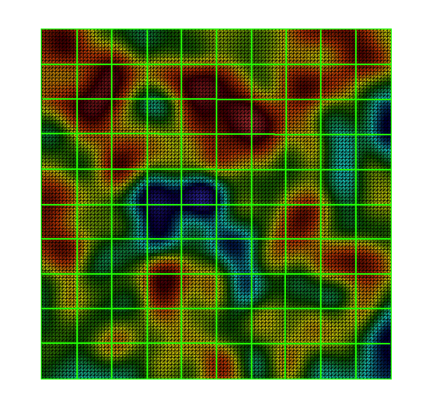
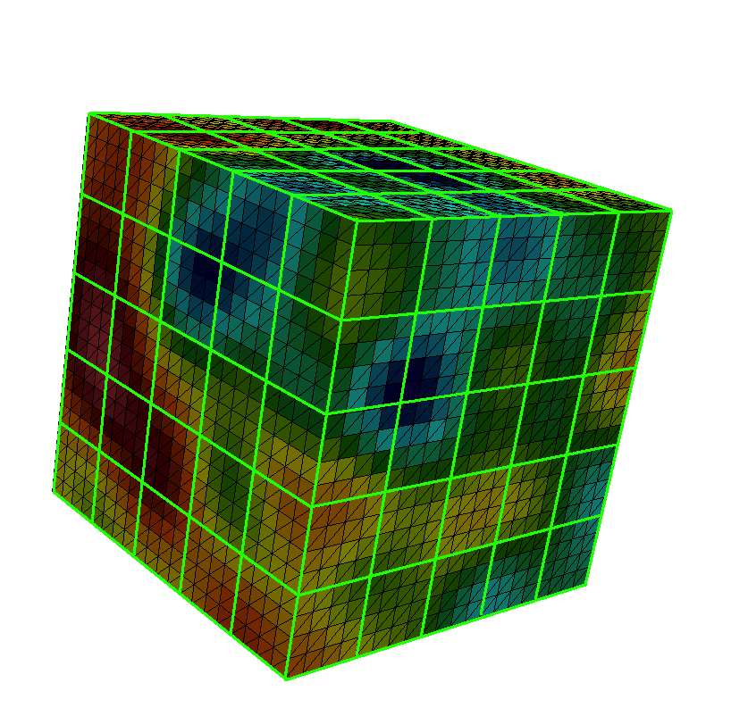
The main idea for solution problem in the stochastic media is to precompute multiscale basis functions using a number of permeability and elastic modulus realizations and use them for the making inexpensive coarse grid calculations.

3.1 Multiscale basis functions for pressure

In the offline computation, we first construct a snapshot space. Construction involves solving the local problem for various choices of input parameters and various boundary conditions. For each fixed parameter $\theta_{r}$ ($r=1,...,N_{r}$), we propose a snapshot space generated by harmonic extensions of $b(\theta_{r};p,q)$

$$\begin{split}b(\theta_{r};\psi_{r,j}^{\omega_{i},\text{snap}},q)&=0\quad x\in\omega_{i},\\ \psi_{r,j}^{\omega_{i},\text{snap}}&=g_{j}(x)\quad x\in\partial\omega_{i},\end{split}$$ (4)

where $g_{j}(x)=\delta_{j,k}$, $\forall k\in J_{h}(\omega_{i})$ ($J_{h}(\omega_{i})$ denotes the fine-grid boundary node on $\partial\omega_{i}$.

We collect all solutions as a snapshot space in the local domain $\omega_{i}$ to define local snapshot space

$$Q^{\omega_{i},\text{snap}}=\text{span}\{\psi_{r,j}^{\omega_{i},\text{snap}}:\,1\leq r\leq N_{r},\,0\leq j\leq N^{\partial\omega_{i}}\},$$

where $N^{\partial\omega_{i}}$ is the number of the fine-grid boundary nodes on $\partial\omega_{i}$.

We reorder the snapshot functions using a single index to create the matrix

$$R_{p}^{\omega_{i},\text{snap}}=\left[\psi_{1}^{\omega_{i},\text{snap}},\ldots,\psi_{M_{p,\text{snap}}}^{\omega_{i},\text{snap}}\right]^{T},$$

where $M_{p,\text{snap}}=N^{\partial\omega_{i}}N_{r}$ denotes the total number of functions to keep in the snapshot construction.

To construct the offline space $Q_{\omega_{i},\text{off}}$, we perform a dimension reduction of the space of snapshots by using an auxiliary spectral decomposition. More precisely, we solve the eigenvalue problem in the space of snapshots:

$$B^{\omega_{i},\text{off}}\Psi_{j}^{\omega_{i},\text{off}}=\lambda_{j}S^{\omega_{i},\text{off}}\Psi_{j}^{\omega_{i},\text{off}},$$ (5)

where

$$\begin{split}B^{\omega_{i},\text{off}}=\{b_{lk}\},\quad b_{lk}&=\int_{\omega_{i}}\overline{k}(x)\,\nabla\psi^{\omega_{i},\text{snap}}_{l},\nabla\psi^{\omega_{i},\text{snap}}_{k}\,dx=R_{p}^{\omega_{i},\text{snap}}\,\overline{B}\,(R_{p}^{\omega_{i},\text{snap}})^{T},\\ S^{\omega_{i},\text{off}}=\{s_{lk}\},\quad s_{lk}&=\int_{\omega_{i}}\overline{k}(x)\,\psi^{\omega_{i},\text{snap}}_{l}\psi^{\omega_{i},\text{snap}}_{k}\,dx=R_{p}^{\omega_{i},\text{snap}}\,\overline{S}\,(R_{p}^{\omega_{i},\text{snap}})^{T}.\end{split}$$

Here

$$\overline{k}(x)=\sum_{r=1}^{N_{r}}t_{r}k(x,\theta_{r}),$$

is independent of $\theta_{r}$ and $t_{j}$ are prescribed non-negative weights. The main objective is to use the offline space to accurately construct a set of multiscale basis functions for each $\theta_{r}$. At the offline stage the bilinear forms are chosen to be parameter-independent, such that there is no need to reconstruct the offline space for each $\theta_{r}$.

We then choose the smallest $M^{\omega_{i}}_{p}$ eigenvalues from Eq. (5) and form the corresponding eigenvectors in the space of snapshots by setting

$$\psi_{j}^{\omega_{i},\text{off}}=(R_{p}^{\omega_{i},\text{snap}})^{T}\Psi_{j}^{\omega_{i},\text{off}},\quad j=1,\ldots,M^{\omega_{i}}_{p}.$$

Finally, we multiply the partition of unity functions $\chi_{i}$ by the eigenfunctions to construct the resulting basis functions

$$\psi_{i,j}=\chi_{i}\psi_{j}^{\omega_{i},\text{off}},\quad 1\leq i\leq N_{v},\quad 1\leq j\leq M^{\omega_{i}}_{p},$$ (6)

where $\chi_{i}$ is the standard linear partition of unity function.

Next, we define the offline space and projection matrix as

$$Q_{H}=\text{span}\{\psi_{i,j}:\,1\leq i\leq N_{c},\,1\leq j\leq M_{p}\},\quad R_{p}=\left[\psi_{1,1},\ldots,\psi_{N_{c},M_{p}}\right]^{T},$$ (7)

where $N_{c}$ is number of coarse mesh nodes and $M_{p}=M^{\omega_{i}}_{p}$ ($i=1,...,N_{c}$).

3.2 Multiscale basis functions for displacements

For construction of multiscale basis functions for displacements we use similar algorithm. We first construct a snapshot space for each parameter $\theta_{r}$ as a harmonic extension of $a(\theta_{r};u,v)$

$$\begin{split}a(\theta_{r};\phi_{r,j}^{\omega_{i},\text{snap}},v)&=0,\quad x\in\omega_{i},\\ \phi_{r,j}^{\omega_{i},\text{snap}}&=g_{j}(x),\quad x\in\partial\omega_{i},\end{split}$$ (8)

where $g_{j}(x)=(\delta_{l,k},0,0)$ or $(0,\delta_{l,k},0)$ or $(0,0,\delta_{l,k})$, $\forall l,k\in\textsl{J}_{h}(\omega)$ ($r=1,...,N_{r}$).

Define local snapshot space

$$V^{\omega_{i},\text{snap}}=\text{span}\{\phi_{r,j}^{\omega_{i},\text{snap}}:\,1\leq r\leq N_{r},\,0\leq j\leq d\cdot N^{\partial\omega_{i}}\},$$

for each subdomain $\omega_{i}$ and $d=2,3$.

We denote the corresponding matrix of snapshot functions, again with similar notation, to be

$$R_{u}^{\omega_{i},\text{snap}}=\left[\phi_{1}^{\omega_{i},\text{snap}},\ldots,\phi_{M_{u,\text{snap}}}^{\omega_{i},\text{snap}}\right]^{T},$$

where $M_{u,\text{snap}}=d\cdot N^{\partial\omega_{i}}\cdot N_{r}$ denotes the total number of functions to keep in the snapshot construction.

Again, we perform a dimension reduction of the space of snapshots by using an auxiliary spectral decomposition. We solve the parameter-independent eigenvalue problem in the space of snapshots

$$A^{\omega_{i},\text{off}}\Phi_{j}^{\omega_{i},\text{off}}=\eta_{j}C^{\omega_{i},\text{off}}\Phi_{j}^{\omega_{i},\text{off}},$$ (9)

where

$$A^{\omega_{i},\text{off}}=R^{u}_{\omega_{i},\text{snap}}\overline{A}(R^{u}_{\omega_{i},\text{snap}})^{T},\quad C^{\omega_{i},\text{off}}=R^{u}_{\omega_{i},\text{snap}}\overline{C}(R^{u}_{\text{snap}})^{T},$$

where $\overline{A}$ and $\overline{C}$ denote fine scale matrices

$$\overline{A}=\{a_{lk}\},\quad a_{lk}=\int_{\omega_{i}}\sigma(x,\phi_{l}):\varepsilon(\phi_{k})\,dx,\quad\overline{C}=\{c_{lk}\},\quad c_{lk}=\int_{\omega_{i}}(\overline{\lambda}(x)+2\overline{\mu}(x))\,\phi_{l}\cdot\phi_{k}\,dx,$$

$$\sigma(x,u)=2\overline{\mu}(x)\varepsilon(u)+\overline{\lambda}(x)\mathop{\rm div}\nolimits u\,\mathcal{I},$$

and $\phi_{k}$ are fine-scale basis functions.

Further, we have

$$\overline{\mu}(x)=\frac{\overline{E}(x)}{2(1+\eta)},\quad\overline{\lambda}(x)=\frac{\overline{E}(x)\eta}{(1+\eta)(1-2\eta)},$$

where

$$\overline{E}(x)=\sum_{r=1}^{N_{r}}t_{r}E(x,\theta_{r}),$$

is independent of $\theta_{r}$ and $t_{r}$ are prescribed non-negative weights.

As before for the fluids flow module, at the offline stage of the mechanics the bilinear forms are chosen to be parameter-independent, such that there is no need to reconstruct the offline space for each $\theta_{r}$.

We then choose the smallest $M_{u}^{\omega_{i}}$ eigenvalues from Eq. (9) and form the corresponding eigenvectors in the space of snapshots by setting

$$\phi_{j}^{\omega_{i},\text{off}}=(R^{u}_{\text{snap}})^{T}\Phi_{j}^{\omega_{i},\text{off}},\quad j=1,\ldots,M_{u}^{\omega_{i}}.$$

Finally, we multiply the linear partition of unity functions $\xi_{i}$ by the eigenfunctions to construct the resulting basis functions

$$\phi_{i,j}=\xi_{i}\phi_{j}^{\omega_{i},\text{off}},\quad 1\leq i\leq N_{c},\quad,1\leq j\leq M_{u}^{\omega_{i}}.$$ (10)

Next, we define the multiscale space and projection matrix as

$$V_{H}=\text{span}\{\phi_{i,j}:\,1\leq i\leq N_{c}\,1\leq j\leq M_{u}\},\quad R_{u}=\left[\phi_{1,1},\ldots,\varphi_{N_{c},M_{u}}\right]^{T},$$ (11)

where $M_{u}=M_{u}^{\omega_{i}}$ ($\forall i=1,...,N_{c}$).

3.3 Global coupling

The multiscale spaces are constructed for both the fluid and mechanics, and we can use them at the global level. Using the matrices

$$R_{p}=\left[\psi_{1,1},\ldots,\psi_{N_{c},M_{p}}\right]^{T},\quad\text{and}\quad R_{u}=\left[\phi_{1,1},\ldots,\phi_{N_{c},M_{u}}\right]^{T},$$

we may write matrix form for the multiscale approximation

$$\begin{split}A^{H}(\theta)u^{H}+G^{H}p^{H}&=0,\\ D^{H}\frac{u^{H}-\check{u}^{H}}{\tau}+M^{H}\frac{p^{H}-\check{p}^{H}}{\tau}+B^{H}(\theta)p^{H}&=F^{H},\end{split}$$ (12)

where

$$A^{H}(\theta)=R_{u}A(\theta)R^{T}_{u},\quad G^{H}=R_{u}G^{h}R^{T}_{p},$$

$$B^{H}(\theta)=R_{p}B^{h}(\theta)R^{T}_{p},\quad M^{H}=R_{p}M^{h}R^{T}_{p},\quad D^{H}=R_{p}D^{h}R^{T}_{u},\quad F^{H}=R_{p}F.$$

Finally, we reconstruct solution on the fine grid by $u^{ms}=R^{T}_{u}u^{H}$, $p^{ms}=R^{T}_{p}p^{H}$.

Note that, the construction of the multiscale basis functions is performed on the offline stage and the same for any random field realization. Construction of basis usually contains two steps: (1) the construction of a snapshot space that will be used to compute an offline space; and (2) the construction of an offline space by performing a dimension reduction in the snapshot space. Multiscale basis functions for pressure and displacement described above are referred to Type 1. One can also use all the fine grid nodal basis as snapshots. This offline space is referred to Type 2.

4 Bayesian Uncertainty Quantification

As noted earlier, in many geomechanical applications a multitude of data observations are measured, such as surface subsidence based on InSar data collected from earth observation [23, 6, 16]. Due to the collection procedures and data processing times involved in the apprehension of such data, these pieces of information are often sparse in time, yet spatially global. This is because only one or two post-processed displacement fields are available per year depending on various observation and processing constraints. Other local sensors may stream relatively constant data of surface subsidence, but only at few sparse random spatial locations. To integrate these observations into the subsurface picture we utilize a Bayesian update framework.

We denote the set of such observations as $F_{obs}$ and want to condition the probability distribution of random fields such as $E$ and $k$ to respect the observed data. We develop an algorithm to sample the permeability and elastic parameters given observed data $F_{obs}$ that include subsidence data. This is accomplished by the well known Bayesian formula where we may relate a new posterior probability distribution given that we have measured information from a likelihood and a prior (usually Gaussian).

4.1 Subsurface Properties Parametrization

To parametrize the subsurface properties, we use the Karhunen-Loéve expansion (KLE) [10, 11]. Let $Y(x,\theta)$ be a stochastic process such that

$$\mathbb{E}\left[\left\|Y\right\|^{2}_{L^{2}(\Omega)}\right]<\infty,$$

where $\mathbb{E}$ is expectation.

$Y(x,\theta)$ can be expand as a general Fourier series

$$Y(x,\theta)=\sum_{k=1}^{\infty}Y_{k}(\theta)\varphi_{k}(x),$$

where $Y_{k}(\theta)=\int_{\Omega}Y(x,\theta)\,\varphi_{k}(x)\,dx$ is the Fourier coefficient in the given $L^{2}$ basis $\{\varphi_{k}\}_{k=1}^{\infty}$. We wish to find an $L^{2}$ basis so that the Fourier coefficients are uncorrelated, or in some sense orthogonal in the expectation. More specifically we require $\mathbb{E}\left[Y_{i}(\theta)Y_{j}(\theta)\right]=0.$ We denote the covariance matrix, usually assumed to be Gaussian in their correlation lengths, to be given as $R(x,y)=\mathbb{E}\left[Y(x,\theta)Y(y,\theta)\right].$ Note that it is symmetric and positive definite, thus, we have that

$$\begin{split}\mathbb{E}\left[Y_{i}(\theta)Y_{j}(\theta)\right]&=\mathbb{E}\left[\int_{\Omega}Y(x,\theta)\varphi_{i}(x)dx\int_{\Omega}Y(y,\theta)\varphi_{j}(y)dy\right]\\ &=\int_{\Omega}\int_{\Omega}R(x,y)\varphi_{i}(x)\varphi_{j}(y)\,dx\,dy=\delta_{ij},\end{split}$$

where $\{\varphi_{k}\}_{k=1}^{\infty}$ are mutually orthogonal eigenfunctions corresponding to $R$. Indeed, we have

$$\int_{\Omega}R(x,y)\varphi_{k}(y)\,dy=\psi_{k}\varphi_{k}(x),\quad k=1,2,\dots,$$

where $\psi_{k}=\mathbb{E}\left[Y^{2}_{k}(\theta)\right]$.

We suppose that the Covariance structure $R(x,y)$ is of the form

$$R(x,y)=\sigma_{R}^{2}\exp\left(-\Delta^{2}\right),$$ (13)

with

$$\Delta^{2}=\frac{|x_{1}-x_{2}|^{2}}{l_{x}^{2}}+\frac{|y_{1}-y_{2}|^{2}}{l_{y}^{2}},$$

for two - dimensional case and

$$\Delta^{2}=\frac{|x_{1}-x_{2}|^{2}}{l_{x}^{2}}+\frac{|y_{1}-y_{2}|^{2}}{l_{y}^{2}}+\frac{|z_{1}-z_{2}|^{2}}{l_{z}^{2}},$$

for three - dimensional case with correlation lengths $l_{x}$, $l_{y}$, $l_{z}$ and variance $\sigma_{R}^{2}$.

We denote the normalized stochastic Fourier coefficients as $\nu_{k}(\theta)=Y_{k}(\theta)/\sqrt{\psi_{k}}$ and write

$$Y(x,\theta)=\sum_{k=1}^{\infty}\sqrt{\psi_{k}}\nu_{k}(\theta)\varphi_{k}(x),$$ (14)

where $\mathbb{E}\left[\nu_{i}(\theta)\right]=0$, $\mathbb{E}\left[\nu_{i}(\theta)\nu_{j}(\theta)\right]=\delta_{ij}$, and $\{\psi_{k},\varphi_{k}(x)\}_{k=1}^{\infty}$ are the eigenpairs associated to the convolution eigenvalue problem. We assume that the eigenvalues $\psi_{k}$ are ordered $\psi_{1}\geq\psi_{2}\geq...$.

In simulations to characterize stochastic process, we keep $L$-leading terms to capture most of the energy of the $Y(x,\theta)$

$$Y_{L}(x,\theta)=\sum_{k=1}^{L}\sqrt{\psi_{k}}\nu_{k}(\theta)\varphi_{k}(x),$$ (15)

with following energy ratio of the approximation

$$e(L)=\frac{E||Y_{L}||^{2}}{E||Y||^{2}}=\frac{\sum_{k=1}^{L}\psi_{k}}{\sum_{k=1}^{\infty}\psi_{k}}.$$

For definition of the permeability and elastic properties, we normalize and rescale random filed to define porosity

$$\phi(x,\theta)=\phi(Y_{L}(x,\theta)),$$ (16)

where $Y_{L}(x,\theta)$ is given by (15) with the corresponding covariance as $R$, eigenfunctions $\varphi_{k}$ and stochastic coefficients as $\nu_{k}$.

We suppose that the permeability as a function of porosity

$$k(x,\theta)=\exp\left(a\,\phi(Y_{L}(x,\theta))\right),$$ (17)

where $a>0$.

The elasticity constants $\lambda$ and $\mu$ are given such that

$$\mu(x,\theta)=\frac{E(x,\theta)}{2(1+\eta)},\quad\lambda(x,\theta)=\frac{E(x,\theta)\eta}{(1+\eta)(1-2\eta)},$$

where the elastic modulus is given by

$$E(x,\theta)=b\left(\frac{1.0-\phi(Y_{L}(x,\theta))}{\phi(Y_{L}(x,\theta))}\right)^{n},$$ (18)

where $n=1.5$ and $b>0$ [38].

4.2 Observable Surface Data

For the case of surface subsidence, the surface displacement is used as the observable data

$$u_{obs}(x,t),\quad x\in\partial\Omega_{surf}$$

where $\partial\Omega_{surf}$ the surface boundary. This data is usually dynamic, but sparse in the spatial extent, with the occasional inclusion of global deformation at sparse time interval snapshots.

Figure 2: Observable surface data of geomechanical subsidence. Spatially sparse, but temporally constant ground motion sensors. Temporally sparse, but spatially global satellite observation.

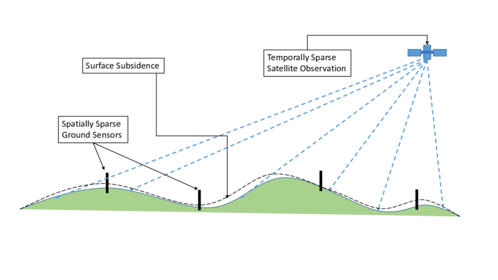
The dynamic data comes from surface sensors at sparse locations throughout the area of interest that continuously monitor displacement in time at sparse locations. While, the global information is available from InSar satellite observation data. However, due to the nature of the collection of this data and the length of time to process the large data sets involved, only snapshots of data are usually available in practical settings. To make this more precise, we suppose that at distinct points $x_{i}\in\partial\Omega_{surf}$, for $i=1,\cdots N^{s}_{data}$, $u_{obs}(x_{i},t)$ is known for all time $t\in[0,T]$. Further, we suppose that at snapshot times $t_{j}$, $j=1,\cdots N^{t}_{data}$, $u_{obs}(x,t_{j})$ is known for all time $x\in\partial\Omega_{surf}$

Suppose that $u_{\theta}(x,t)$ is the displacement computed using properties $E(\theta)$ and $k(\theta)$, then we define our data misfit as

$$\left\|F_{obs}-F_{\theta}\right\|^{2}=\sum_{i=1}^{N^{s}_{data}}\int_{0}^{T}|u_{obs}(x_{i},t)-u_{\theta}(x_{i},t)|^{2}dt+\sum_{j=1}^{N^{t}_{data}}\int_{\partial\Omega_{surf}}|u_{obs}(x,t_{j})-u_{\theta}(x,t_{j})|^{2}ds,$$ (19)

where $ds$ is the surface measure.

4.3 Single-stage Metropolis - Hastings Algorithm

The posterior distribution $\pi(\theta)$ can be expressed as

$$\pi(\theta)=p(\theta|F_{obs})\propto p(F_{obs}|\theta)\,p(\theta),$$ (20)

where $p(F_{obs}|\theta)$ is the likelihood and $p(\theta)$ is the prior distribution.

Given a set of observed data $F_{obs}$ and heterogeneous field parameter data $\theta$ we write $F(\theta)$ to be the corresponding simulated data (on the fine-grid) i.e. subsidence displacement or pressures. Due to uncertainty in the model and measurements, we suppose that the error is such that

$$F_{obs}-F(\theta)=\varepsilon,$$

where $\varepsilon$ is random normal with mean $0$ and variance $\sigma_{f}^{2}$, or in standard notation $\varepsilon$ follows ${\cal N}(0,\sigma_{f}^{2})$. Thus, we will write the posterior as

$$p(\theta|F_{obs})\propto\exp\left(-\frac{\left\|F(\theta)-F_{obs}\right\|^{2}}{\sigma_{f}^{2}}\right)p(\theta).$$ (21)

Let $q(\theta|\theta_{n})$ be the instrumental distribution that is used to choose the next fields $\theta$ given the previous properties $\theta_{n}$. We consider a random walk samplers for the transitional probability distribution $q(\theta|\theta_{n})$ and set $q(\theta|\theta_{n})=\theta_{n}+\delta\cdot r$, where $r$ is a Gaussian random variable with zero mean and variance 1.

The single - stage Metropolis - Hastings algorithm:

1. Given $\theta_{n}$, generate new proposal $\theta$, from $q(\theta|\theta_{n})$.

2. Solve forward problem, using $\theta$, generate observable $F(\theta)$.

3. Determine the acceptance probability from

   $$\text{Prob}(\theta_{n}|\theta)=\text{min}\left(1,\frac{q(\theta_{n}|\theta)\,p(\theta|F_{obs})}{q(\theta|\theta_{n})\,p(\theta_{n}|F_{obs})}\right),$$ (22)

   and take

   $$\theta_{n+1}=\left\{\begin{matrix}\theta&\text{with probability}\quad\text{Prob}(\theta_{n}|\theta),\\ \theta_{n}&\text{with probability}\quad 1-\text{Prob}(\theta_{n}|\theta).\end{matrix}\right.$$

For symmetric $q(\cdot|\cdot)$, we have

$$\text{Prob}(\theta_{n}|\theta)=\text{min}\left(1,\exp\left(-\frac{E(\theta)-E(\theta_{n})}{\sigma_{f}^{2}}\right)\right),$$

with $E(\theta)=\left\|F(\theta)-F_{obs}\right\|^{2}$ and $E(\theta_{n})=\left\|F(\theta_{n})-F_{obs}\right\|^{2}$.

It is well known that the above algorithm is very costly due to the expense of having to solve the fine-scale solution and the low acceptance rate of new proposals. A method to save computational cost is to use a coarse-scale model or/and machine learning technique as a preconditioning phase to cheaply reject proposals. Then, if the proposals is accepted on the cheap first-stage, run a fine-scale simulation and generate new acceptance-rejection probabilities. This two-stage procedure has been utilized in various other applications [10, 11, 15].

4.4 Two-stage Metropolis - Hastings Algorithm

Let

$$p^{*}(\theta|F_{obs})\propto\exp\left(-\frac{E^{*}(\theta)}{\sigma_{c}^{2}}\right),$$ (23)

where $E^{*}(\theta)=\left\|F^{*}(\theta)-F_{obs}\right\|^{2}$ and $\sigma_{c}^{2}$ is the precision associated with the approximate model.

Here $F^{*}(\theta)$ denotes the simulated data that generated using

• MS: coarse scale simulations (multiscale solver),

• ML: machine learning techniques,

The two - stage Metropolis - Hastings algorithm:

1. Given $\theta_{n}$, generate new proposal $\theta^{\prime}$, from $q(\theta^{\prime}|\theta_{n})$.

2. First stage:

   1. Generate observable $F^{*}(\theta^{\prime})$ for given $\theta^{\prime}$ using forward multiscale solver (MS) or machine learning technique (ML).

   2. Determine the acceptance probability from

      $$g(\theta_{n}|\theta^{\prime})=\text{min}\left(1,\frac{q(\theta_{n}|\theta^{\prime})p^{*}(\theta^{\prime}|F_{obs})}{q(\theta^{\prime}|\theta_{n})p^{*}(\theta_{n}|F_{obs})}\right),$$ (24)

      and take

      $$\theta=\left\{\begin{matrix}\theta^{\prime}&\text{with probability}\quad g(\theta_{n}|\theta),\\ \theta_{n}&\text{with probability}\quad 1-g(\theta_{n}|\theta).\end{matrix}\right.$$

3. Second stage, if accepted:

   1. Solve fine-scale forward problem using $\theta$ and generate observable $F(\theta)$.

   2. Determine the acceptance probability from

      $$\rho(\theta_{n}|\theta)=\text{min}\left(1,\frac{p^{*}(\theta_{n}|F_{obs})p(\theta|F_{obs})}{p^{*}(\theta|F_{obs})p(\theta_{n}|F_{obs})}\right),$$ (25)

      and take

      $$\theta_{n+1}=\left\{\begin{matrix}\theta&\text{with probability}\quad\rho(\theta_{n}|\theta),\\ \theta_{n}&\text{with probability}\quad 1-\rho(\theta_{n}|\theta).\end{matrix}\right.$$

Here, we have

$$g(\theta_{n}|\theta^{\prime})=\text{min}\left(1,\exp\left(-\frac{E^{*}(\theta^{\prime})-E^{*}(\theta_{n})}{\sigma_{c}^{2}}\right)\right),$$

and

$$\rho(\theta_{n}|\theta)=\text{min}\left(1,\frac{p^{*}(\theta_{n}|F_{obs})p(\theta|F_{obs})}{p^{*}(\theta|F_{obs})p(\theta_{n}|F_{obs})}\right)=\text{min}\left(1,\exp\left(-\frac{E(\theta)-E(\theta_{n})}{\sigma_{f}^{2}}+\frac{E^{*}(\theta)-E^{*}(\theta_{n})}{\sigma_{c}^{2}}\right)\right).$$

If $E^{*}(\theta)$ is strongly correlated with $E(\theta)$, then the acceptance probability $\rho$ could be close to 1 for certain choice of $\sigma_{c}$ [11].

To Generate observable $E^{*}(\theta^{\prime})$ for given $\theta^{\prime}$ using forward multiscale solver (MS), we use following steps:

• Offline stage. Construction of the projection matrices $R_{p}$ and $R_{u}$.

• Online stage. For given $\theta^{\prime}$:

  1. generate a coarse grid system using preconstructed projection matrices,

  2. solve time-depended coarse grid system (12),

  3. find observable data $u_{obs}(\theta^{\prime})$ on the surface boundary from multiscale solution,

  4. generate $E^{*}(\theta^{\prime})$.

In machine learning technique (ML), we have following steps:

• Offline stage. Dataset generation and neural networks training.

• Online stage. For given $\theta^{\prime}$:

  1. predict observable data $u_{obs}(\theta^{\prime})$ on the surface boundary using trained neural networks,

  2. generate $E^{*}(\theta^{\prime})$.

We construct a neural network (NN) for displacements in each direction $x,y$ and $z$. Therefore, we train two NNs for two-dimensional problems (2D) and three NNs for three-dimensional problems (3D) [36]. In ML, we directly predict an observable data for given $\theta^{\prime}$, without solution of the forward problem.

To construct a neural network for prediction of the observable data, we generate a dataset by the solution of the forward problems using a multiscale solver for some number of random coefficient $\theta_{r}$ ($r=1,...,N_{r}$)

$$\text{ Dataset: }\{(X_{r},Q_{r}),\,r=1,...,N_{r}\}.$$

where $X_{r}=\theta_{r}$ and $Q_{r}=u_{obs}(\theta_{r})$ are the input data and output data. The input field is represented as a two-dimensional array for the two-dimensional problem and as a three-dimensional array for three-dimensional problems. The dataset is re-scaled to fall within the range $0$ to $1$.

We use a convolutional neural network, where several convolutional, pooling, and activation layers are stacked with several fully-connected layers with dropout. Training of the machine learning algorithms is performed using mean square loss function (MSE). Implementation of the machine learning method is based on the library Keras [9] with TensorFlow backend [1] and performed on the GPU. The machine-learning algorithm learns dependence between global random coefficients ($\theta$) and observable data $u_{obs}(\theta)$.

5 Numerical results

In order to investigate the proposed method, we perform the following tests:

• In Section 5.1, we consider multiscale solver for three test cases in 2D and 3D formulations. We show the relative errors between reference (fine-grid) solution and GMsFEM solution with different numbers of the multiscale basis functions. Also, we present a solution time of the proposed multiscale method.

• In Section 5.2, we consider MCMC method with GMsFEM preconditioning. We start with tests of multiscale solver, where we present errors for pressure and displacements for 100 random realizations. Next, we demonstrate correlation between $E(\theta)$ (fine grid solver) and $E^{*}(\theta)$ (multiscale solver with different number of basis functions). After that, we present results for the two-stage MCMC method with GMsFEM preconditioning for 2D and 3D test problems. We investigate the influence of the method parameters on the numbers of the accepted fields and number of the fields that pass the first stage in the two-dimensional formulation. Some figures of accepted fields with corresponded solutions are presented.

• In Section 5.3, we consider the preconditioned MCMC method using a machine learning technique. We start with the demonstration of the neural network architectures for 2D and 3D problems, and we use them for the prediction of the observable data. Next, we demonstrate correlation between $E(\theta)$ (fine grid solver) and $E^{*}(\theta)$ (machine learning method). After that, we present results for the preconditioned MCMC method, where we took an observable data for three test cases considered in Section 5.1. We shown results for both preconditioning approaches: (MS) multiscale solver based on GMSFEM and (ML) machine learning technique. Finally, we discuss the computational advantage of the method.

5.1 Multiscale method

In this section, we present numerical examples to demonstrate the performance of the multiscale method for computing the solution of the poroelasticity problem with random heterogeneous properties.

(a) $k(x)$ for Case 1, 2 and 3 (from left to right).

(b) $E(x)$ for Case 1, 2 and 3 (from left to right).

Figure 3: Random permeability $k$ and elastic modulus $E$. Two - dimensional problem (2D). Case 1, 2 and 3 (from left to right). (a) permeability, $k(x)$. (b) elastic modulus, $E(x)$.

(a) $p$ for Case 1, 2 and 3 (from left to right).

(b) $u_{m}$ for Case 1, 2 and 3 (from left to right).

Figure 4: Numerical results for random permeability $k$ and elastic modulus $E$. Case 1, 2 and 3 (from left to right). Fine grid solution of two - dimensional problem (2D). (a) pressure, $p$. (b) displacement, $u_{m}$.

(a) $k(x)$ for Case 1, 2 and 3 (from left to right).

(b) $E(x)$ for Case 1, 2 and 3 (from left to right).

Figure 5: Random permeability $k$ and elastic modulus $E$. Three - dimensional problem (3D). Case 1, 2 and 3 (from left to right). (a) permeability, $k(x)$. (b) elastic modulus, $E(x)$.

(a) $p$ for Case 1, 2 and 3 (from left to right).

(b) $u_{m}$ for Case 1, 2 and 3 (from left to right).

Figure 6: Numerical results for random permeability $k$ and elastic modulus $E$. Case 1, 2 and 3 (from left to right). Fine grid solution of three - dimensional problem (3D). (a) pressure, $p$. (b) displacement, $u_{m}$.

2D
$M_{+}$	$M_{p}$	$M_{u}$	$DOF_{c}$	$e_{p}$ (%)	$e_{u}$ (%)
Case 1
0	1	2	363	7.532	6.413
1	2	3	605	4.800	4.048
2	3	4	847	1.368	2.076
3	4	5	1089	0.940	1.634
4	5	6	1331	0.635	1.146
6	7	8	1815	0.303	0.840
8	9	10	2299	0.182	0.661
Case 2
0	1	2	363	2.142	2.953
1	2	3	605	1.151	2.127
2	3	4	847	0.641	1.649
3	4	5	1089	0.529	1.309
4	5	6	1331	0.234	0.822
6	7	8	1815	0.117	0.552
8	9	10	2299	0.068	0.440
Case 3
0	1	2	363	4.635	6.847
1	2	3	605	2.760	4.303
2	3	4	847	0.778	2.005
3	4	5	1089	0.492	1.579
4	5	6	1331	0.343	0.993
6	7	8	1815	0.198	0.694
8	9	10	2299	0.124	0.535

3D
$M_{+}$	$M_{p}$	$M_{u}$	$DOF_{c}$	$e_{p}$ (%)	$e_{u}$ (%)
Case 1
0	1	3	864	4.369	5.477
1	2	4	1296	2.727	4.343
2	3	5	1728	1.914	3.716
3	4	6	2160	1.356	3.220
4	5	7	2592	0.853	2.672
6	7	9	3456	0.453	1.904
8	9	11	4320	0.352	1.619
Case 2
0	1	3	864	6.000	3.653
1	2	4	1296	5.194	3.235
2	3	5	1728	3.185	2.700
3	4	6	2160	2.144	2.455
4	5	7	2592	0.912	2.114
6	7	9	3456	0.571	1.693
8	9	11	4320	0.452	1.443
Case 3
0	1	3	864	3.430	4.520
1	2	4	1296	2.752	3.997
2	3	5	1728	1.709	3.318
3	4	6	2160	1.129	3.071
4	5	7	2592	0.730	2.841
6	7	9	3456	0.487	2.331
8	9	11	4320	0.377	1.905

Table 1: Numerical results for random permeability $k$ and elastic modulus $E$. Case 1, 2 and 3 (from left to right). Type 1 multiscale basis functions, $M_{p}=1+M_{+}$, $M_{u}=d+M_{+}$ and $DOF_{c}=(M_{p}+M_{u})\cdot N_{c}$. Left: two - dimensional problem, $d=2$ ($N_{c}=121$ and $DOF_{f}=30603$). Right: three - dimensional problem, $d=3$ ($N_{c}=216$ and $DOF_{f}=37044$)

2D
$M_{+}$	$M_{p}$	$M_{u}$	$DOF_{c}$	$e_{p}$ (%)	$e_{u}$ (%)
Case 1
0	1	2	363	7.532	6.413
1	2	3	605	5.737	4.669
2	3	4	847	2.396	2.793
3	4	5	1089	1.548	1.796
4	5	6	1331	1.102	1.300
6	7	8	1815	0.639	0.481
8	9	10	2299	0.364	0.272
Case 2
0	1	2	363	2.142	2.953
1	2	3	605	1.219	1.847
2	3	4	847	0.703	1.430
3	4	5	1089	0.596	1.085
4	5	6	1331	0.380	0.708
6	7	8	1815	0.180	0.220
8	9	10	2299	0.101	0.146
Case 3
0	1	2	363	4.635	6.847
1	2	3	605	2.397	4.294
2	3	4	847	0.842	2.596
3	4	5	1089	0.570	1.641
4	5	6	1331	0.379	1.109
6	7	8	1815	0.218	0.336
8	9	10	2299	0.149	0.224

3D
$M_{+}$	$M_{p}$	$M_{u}$	$DOF_{c}$	$e_{p}$ (%)	$e_{u}$ (%)
Case 1
0	1	3	864	4.369	5.477
1	2	4	1296	2.750	4.045
2	3	5	1728	1.707	3.530
3	4	6	2160	1.348	3.052
4	5	7	2592	0.906	2.691
6	7	9	3456	0.467	2.329
8	9	11	4320	0.358	1.962
Case 2
0	1	3	864	6.000	3.653
1	2	4	1296	4.940	3.224
2	3	5	1728	3.585	2.731
3	4	6	2160	2.514	2.496
4	5	7	2592	1.805	2.327
6	7	9	3456	1.042	2.052
8	9	11	4320	0.830	1.694
Case 3
0	1	3	864	3.430	4.520
1	2	4	1296	2.705	3.991
2	3	5	1728	1.613	3.197
3	4	6	2160	1.142	2.659
4	5	7	2592	0.812	2.544
6	7	9	3456	0.554	2.356
8	9	11	4320	0.454	2.062

Table 2: Numerical results for random permeability $k$ and elastic modulus $E$. Case 1, 2 and 3 (from left to right). Type 2 multiscale basis functions, $M_{p}=1+M_{+}$, $M_{u}=d+M_{+}$ and $DOF_{c}=(M_{p}+M_{u})\cdot N_{c}$. Left: two - dimensional problem, $d=2$ ($N_{c}=121$ and $DOF_{f}=30603$). Right: three - dimensional problem, $d=3$ ($N_{c}=216$ and $DOF_{f}=37044$)

2D
$M_{+}$	$M_{p}$	$M_{u}$	$DOF_{c}$	Time (sec)
fine grid			30603	6.211
0	1	2	363	0.350
1	2	3	605	0.587
2	3	4	847	0.833
3	4	5	1089	1.171
4	5	6	1331	1.611
6	7	8	1815	2.767
8	9	10	2299	4.569

3D
$M_{+}$	$M_{p}$	$M_{u}$	$DOF_{c}$	Time (sec)
fine grid			37044	158.745
0	1	3	864	2.525
1	2	4	1296	4.940
2	3	5	1728	9.633
3	4	6	2160	16.285
4	5	7	2592	20.495
6	7	9	3456	38.951
8	9	11	4320	69.322

Table 3: Solution time for Case 3. Type 2 multiscale basis functions. Left: two - dimensional problem, $d=2$. Right: three - dimensional problem, $d=3$

We consider two and three-dimensional model problems in domain $\Omega=[0,1]^{d}$ with $d=2,3$:

• Two - dimensional problem (2D). Coarse grid contains 121 nodes ($10\times 10$) and the fine grid has 10201 nodes.

• Three - dimensional problem (3D). Coarse grid contains of 216 nodes ($5\times 5\times 5$) and fine grid has 9261 nodes.

The coarse grid and fine grid are presented in Figure 1.

We perform simulations for $T_{max}=0.001$ with 20 time steps. As an initial condition, we set $p_{0}=0$ and impose the following boundary conditions:

$$u_{x}=0,\quad\sigma_{y}=0,\quad\sigma_{z}=0,\quad x=0,$$

$$\sigma_{x}=0,\quad u_{y}=0,\quad\sigma_{z}=0,\quad y=0,$$

$$\sigma_{x}=0,\quad\sigma_{y}=0,\quad u_{z}=0,\quad z=0,$$

$$\sigma\cdot n=0,\quad x,y,z=1,$$

and

$$q\cdot n=\gamma(p-p_{1}),\quad y=1,$$

$$q\cdot n=0,\quad y\neq 1,$$

with $\gamma=10^{4}$ and $p_{1}=1.0$.

The high dimensional heterogeneity is represented using Karhunen-Loéve expansion. Random heterogeneous porosity fields are generated using $L=200$ basis functions ($Y_{L}(x,\theta)$) with exponential covariance ($l_{x}=l_{y}=l_{z}=0.2$ and $\sigma_{R}^{2}=2$)

$$\phi(x,\theta)=\phi(Y(x,\theta)),$$

with normalization, that give $\phi\in[0.05,0.2]$.

Heterogeneous permeability and elasticity modulus fields are given by

$$k(x,\theta)=\exp\left(a\,\phi(x,\theta)\right),$$

$$E(x,\theta)=b\left(\frac{1.0-\phi(x,\theta)}{\phi(x,\theta)}\right)^{m},$$

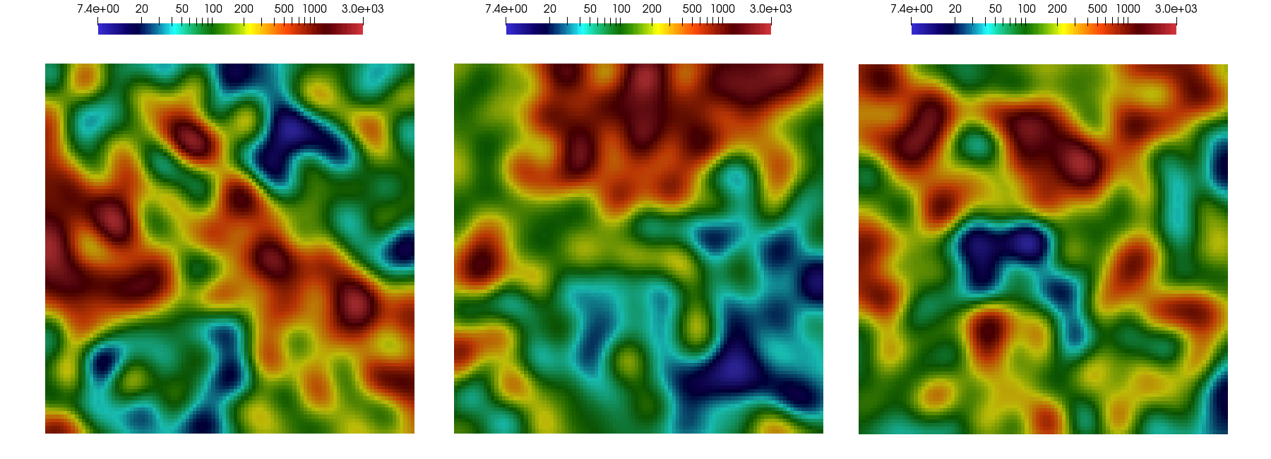
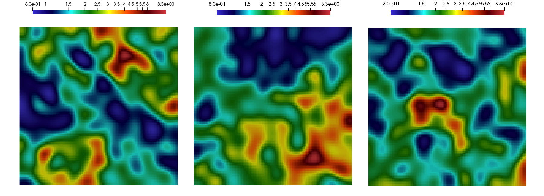
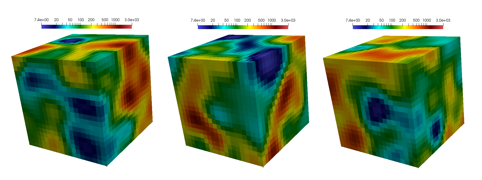
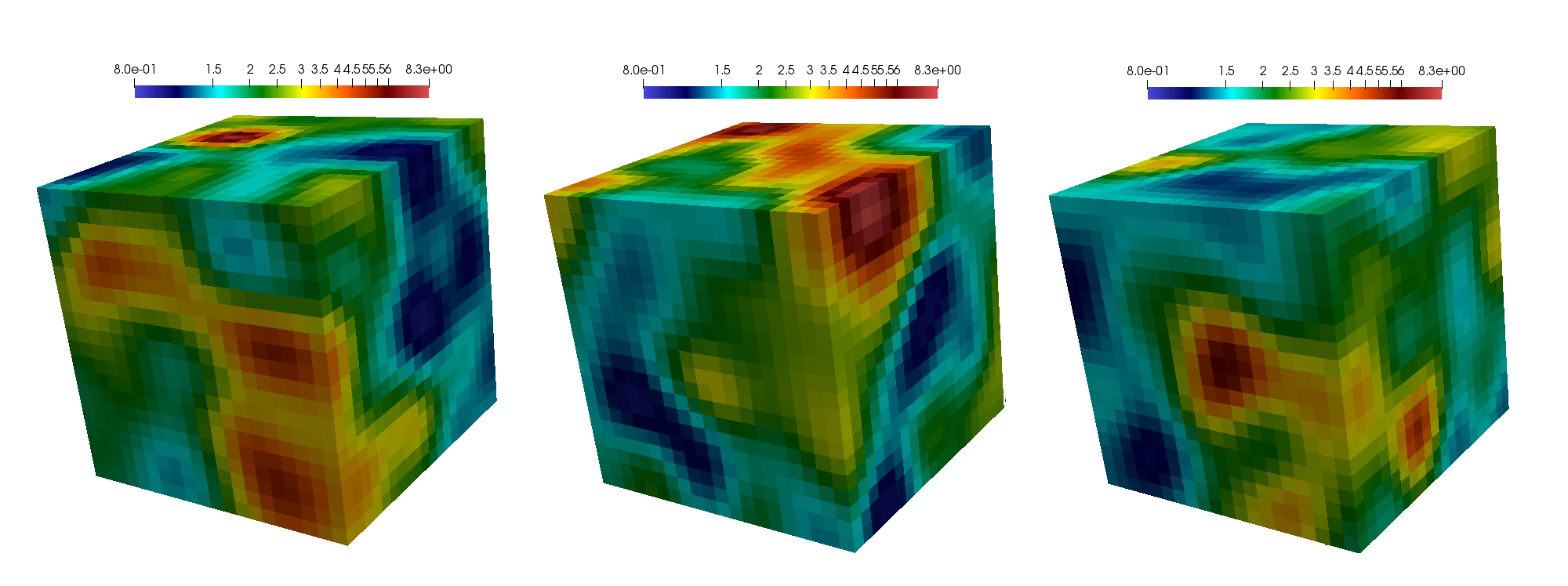
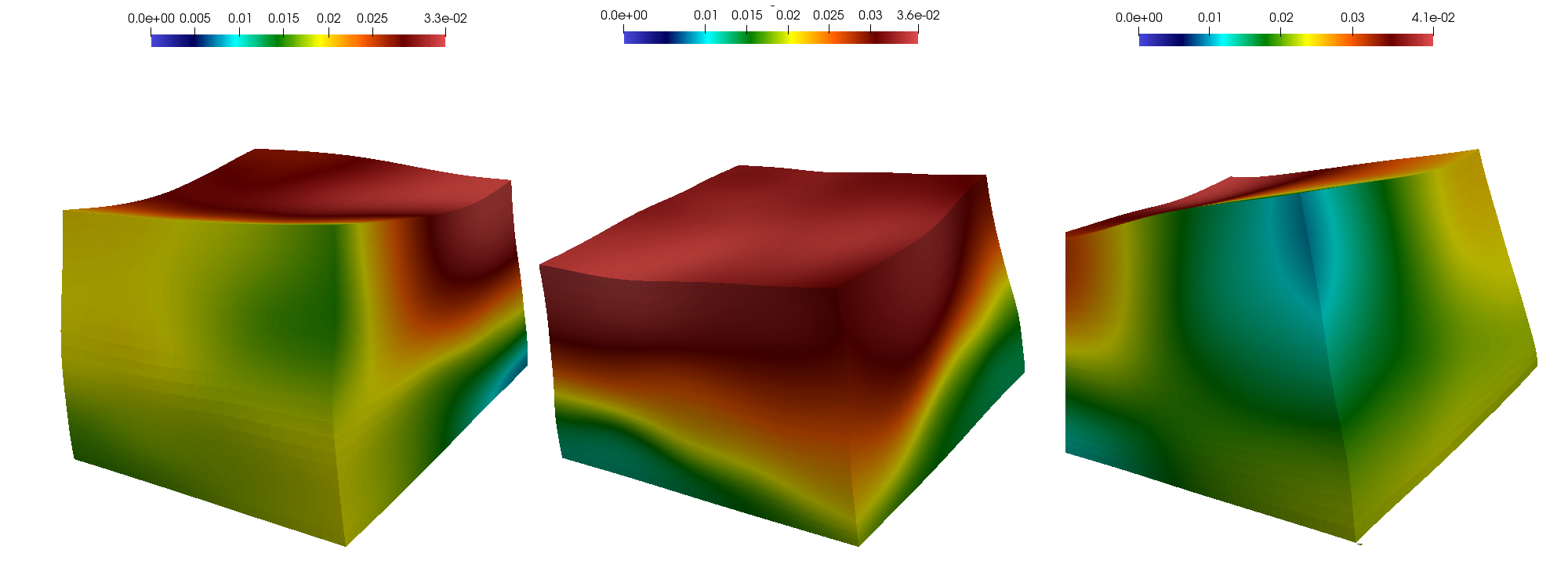
with $a=40$, $b=0.1$ and $m=1.5$ [38]. The Biot modulus is $M=1.0$, fluid viscosity is $\nu=1$, fluid-solid coupling constant is $\alpha=0.1$, the Poisson’s ratio is $\eta=0.3$. Permeability field and elastic modulus are shown in Figure 3 for 2D problems and in Figure 5 for 3D problems. We consider three test cases (Case 1, 2 and 3 are depicted from left to right). All permeabilities and elastic modulus are depicted in the log scale.

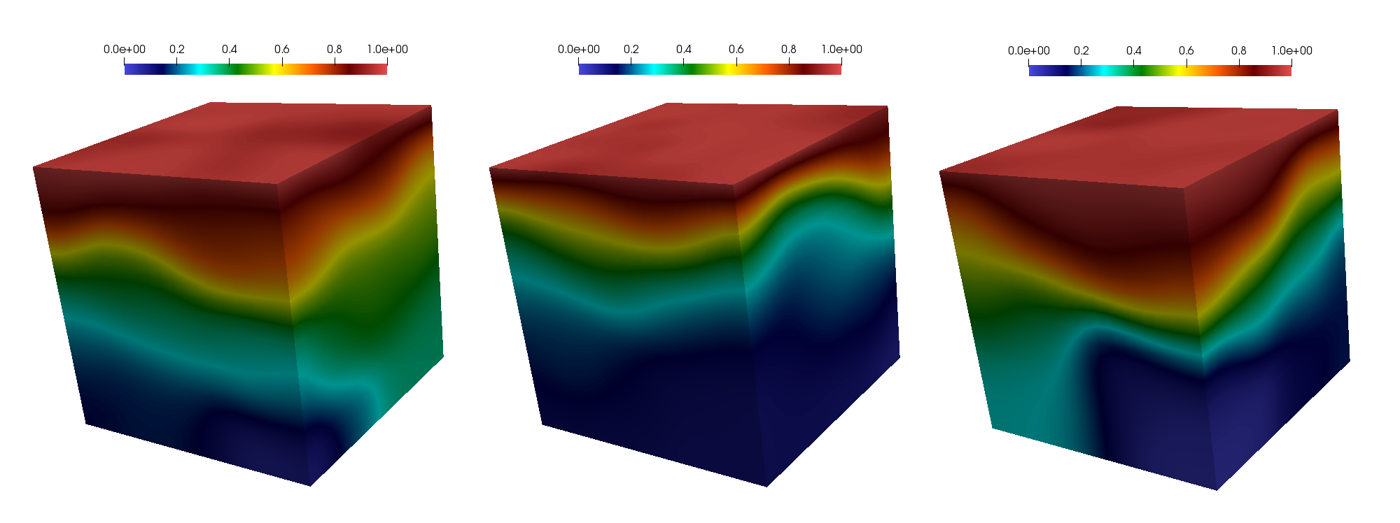
The reference solution computed by a standard finite element method with linear basis functions for pressure and displacements on the fine grid. The reference pressure and the displacement fields at final time are presented in Figures 4 and 6.

To compare a multiscale solution, we calculate relative errors in $L^{2}$ norm in %

$$e_{p}=\sqrt{\frac{\int_{\Omega}(p^{ms}-p,p^{ms}-p)\,dx}{\int_{\Omega}(p,p)\,dx}}\cdot 100\%,$$

$$e_{u}=\sqrt{\frac{\int_{\Omega}(u^{ms}-u,u^{ms}-u)\,dx}{\int_{\Omega}(u,u)\,dx}}\cdot 100\%,$$

where $p^{ms}$ and $u^{ms}$ are multiscale solutions, $p$ and $u$ are reference solutions.

For multiscale basis construction on the offline stage, we use a 10 random permeability and elastic fields. We present numerical results in Tables 1 and 2 for Type 1 and 2 multiscale basis functions. $DOF_{c}$ and $DOF_{f}$ are degrees of freedom for multiscale and reference (fine grid) solutions. $M_{p}$ and $M_{u}$ are the number of the multiscale basis functions for pressure and displacements, respectively. Varying the basis functions in both pressure and displacement multiscale spaces we presented the errors at the final times. We note that the first basis for pressure is standard linear basis function because the first eigenvalue of the local spectral problem is constant. Similarly for displacements, the first $d$ basis functions are standard linear basis functions. $M_{+}$ is used to denote the number of the additional spectral basis functions calculated using algorithm presented in Section 3. Therefore, $M_{p}=1+M_{+}$, $M_{u}=d+M_{+}$ and $DOF_{c}=(M_{p}+M_{u})\cdot N_{c}$, where $N_{c}$ is the number of coarse grid nodes. For two - dimensional problem, we have $N_{c}=121$ and $DOF_{f}=30603$. For three - dimensional problem, we have $N_{c}=216$ and $DOF_{f}=37044$. We can obtain good multiscale solution when we take sufficient number of multiscale basis functions for pressure and for displacements. For $M_{+}=2$, we have near $1-3\%$ of errors in two - dimensional and three-dimensional problems for all cases. In Case 3 of heterogeneous permeability field, we have $0.7$ % of pressure error and $2.0$ % of displacement error in two-dimensional problems with 3 multiscale basis functions for pressure and 4 multiscale basis functions for displacements $M_{+}=2$. In this case, we reduce size of the system from $DOF_{f}=30603$ to $DOF_{c}=847$. For three - dimensional problem, we have $1.7$ % of pressure error and $3.3$ % of displacement error with 3 basis functions for pressure and 5 basis functions for displacements ($M_{+}=2$). We reduce size of the system from $DOF_{f}=37044$ to $DOF_{c}=1728$.

In Table 3, we present solution time for the coarse grid and fine grid solvers for Case 3. Solution time of the fine grid solver is $6.2$ second for two - dimensional problem ($DOF_{f}=30603$) and $158.7$ second for the three-dimensional problem ($DOF_{f}=37044$). When we use a multiscale method for the solution with $M_{+}=2$, we solve two - dimensional problem by $0.8$ seconds ($DOF_{c}=847$) and three-dimensional problem by $9.6$ seconds ($DOF_{c}=1728$). We see that a smaller number of basis functions give a coarse grid system with a smaller size and therefore solution time is faster. Here for the solution of the coarse and fine grid systems, we used a direct solver (default solver in FEniCS [21]). Note that, the solution time doesn’t include a time of multiscale basis construction because they are constructed on the offline stage as precalculations.

5.2 Preconditioned MCMC using GMsFEM

In this section, we present results for the Two-stage MCMC method. MCMC simulations on the fine grid (single-stage) are generally very computationally expensive because each proposal requires solving a forward coupled poroelasticity problem over a large time interval. In presented preconditioned MCMC simulations, we use inexpensive computations in the first stage. Preconditioning procedure is performed using

1. MS multiscale solver based on GMSFEM,

2. ML machine learning technique.

Note that, the Preconditioning procedure should be inexpensive, but not necessarily very accurate. We start with a multiscale solver with a small number of multiscale basis functions. As we showed above, the size of the coarse grid system ($DOF_{c}$) depends on a number of multiscale basis functions. The multiscale basis functions are constructed only once on the offline stage, and we use them for all proposed permeability and elastic modulus without online recalculations.

(a) 2D, $e_{p}$ (%)

(b) 3D, $e_{p}$ (%)

(c) 2D, $e_{u}$ (%)

(d) 3D, $e_{u}$ (%)

Figure 7: Multiscale method errors for 100 random realizations of heterogeneous filed for $M_{+}=0,1,2,4$ and $8$. First row: pressure relative errors in %. Second row: displacement relative errors in %. Left: two - dimensional problem. Right: three - dimensional problem.

(a) 2D

(b) 3D

Figure 8: Cross-plot between ${E(\theta)}$ (fine scale) and ${E^{*}(\theta)}$ (multiscale solver, MS) for $M_{+}=0,1,2,4$ and $8$. For given observation data. (a) two - dimensional problem. (b) three - dimensional problem.

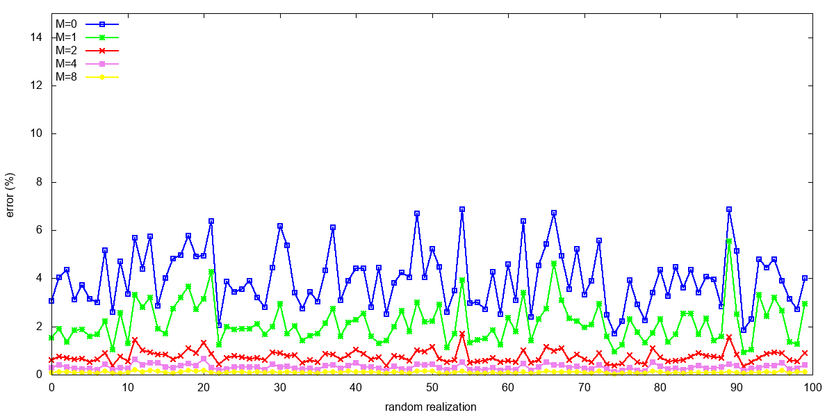
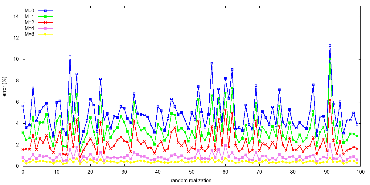
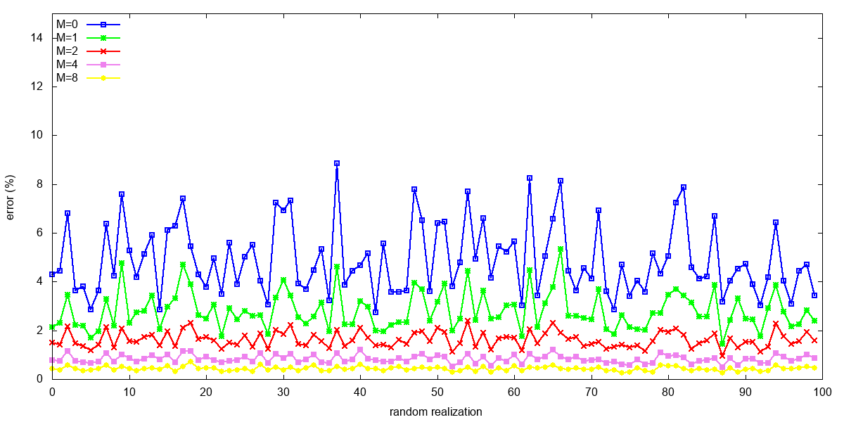
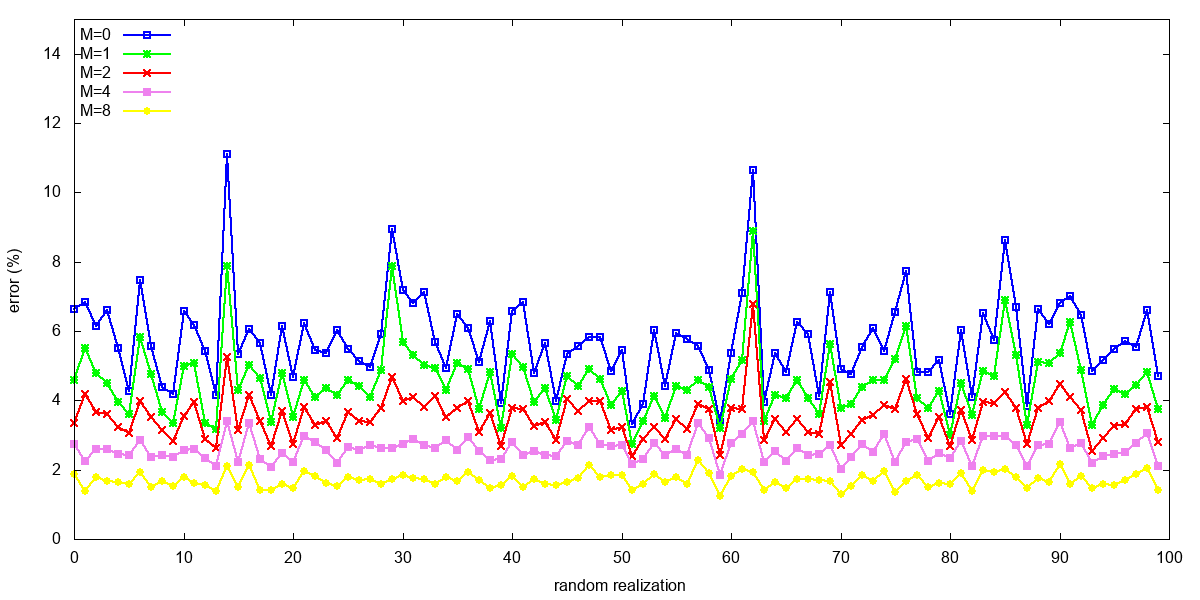
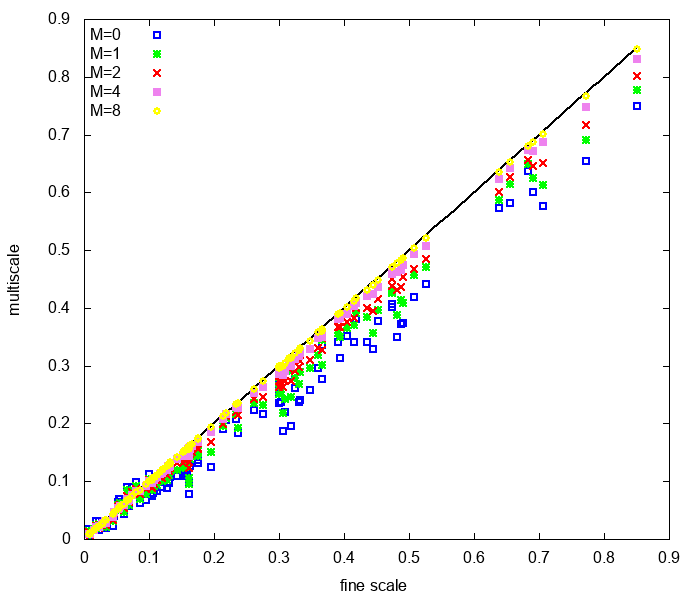
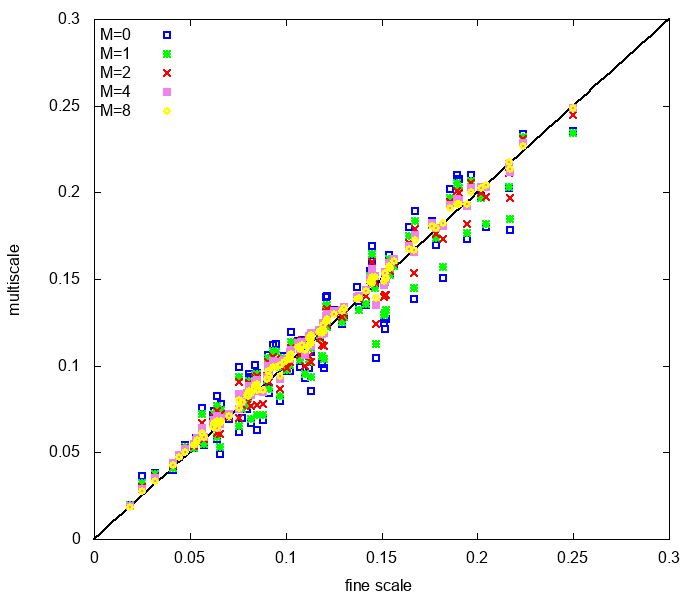
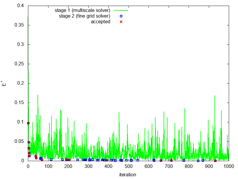
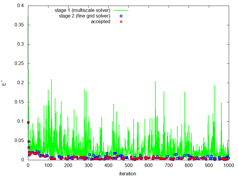
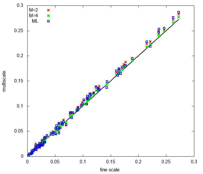
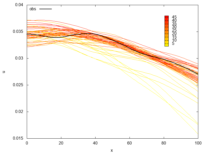
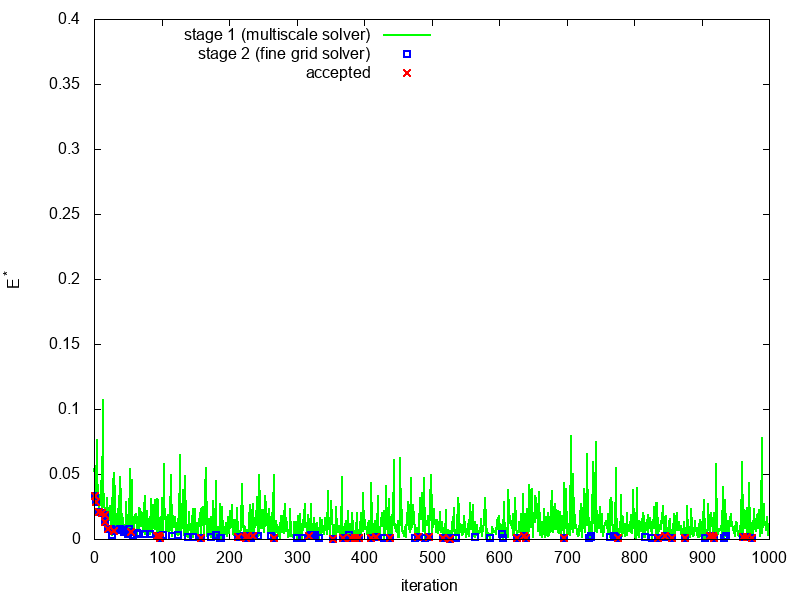
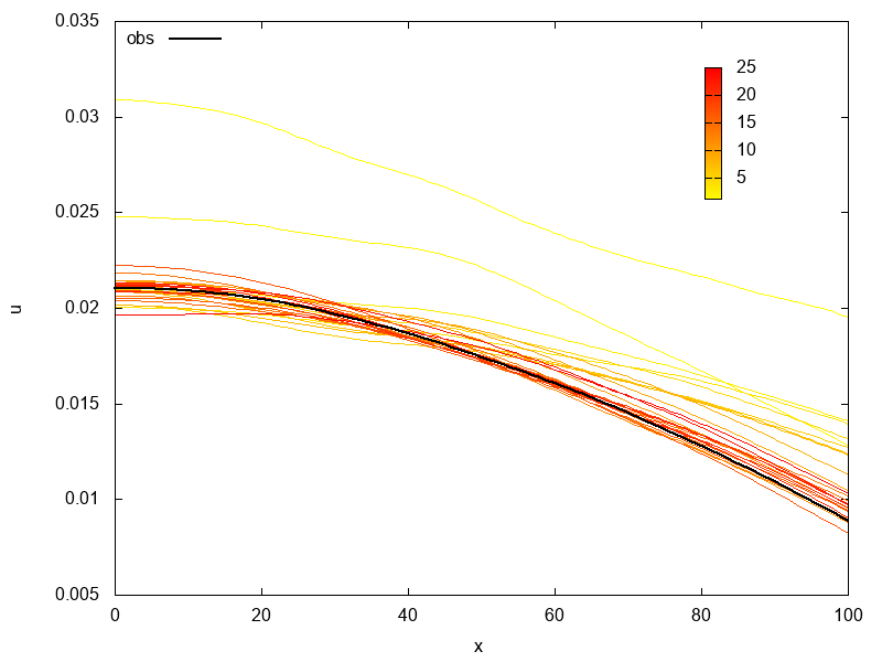
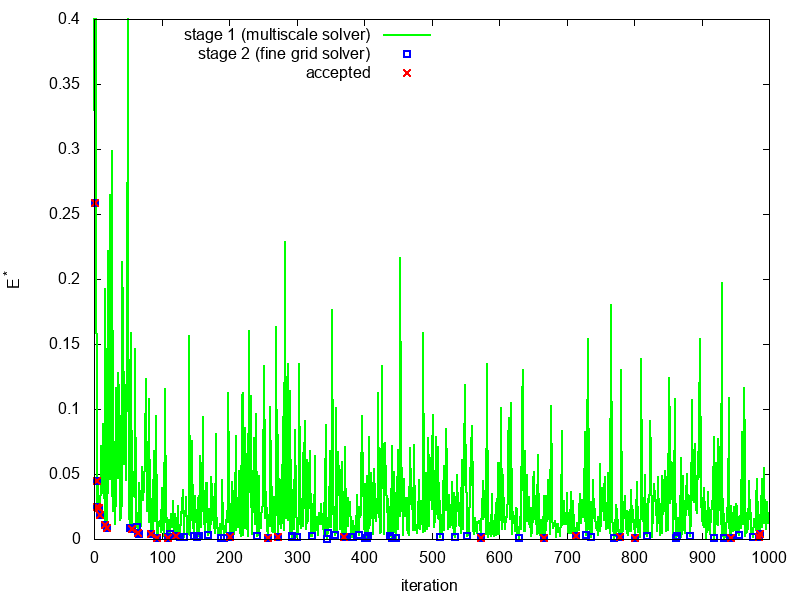
We present results for the proposed multiscale solver (MS) for 100 random realizations of the heterogeneous fields, $\theta_{r}$. Relative errors for pressure and displacements are presented in Figure 7. In Figure 8, we plot $E(\theta)$ against $E^{*}(\theta)$ to demonstrate correlation between ${E^{*}(\theta)}$ and ${E(\theta)}$ for 100 realizations of random fields. Here we use a relative difference between observation data and proposed solution for given $\theta$

$$E^{*}(\theta)=\frac{||F^{*}(\theta)-F_{obs}||^{2}}{||F_{obs}||^{2}},\quad E(\theta)=\frac{||F(\theta)-F_{obs}||^{2}}{||F_{obs}||^{2}},$$ (26)

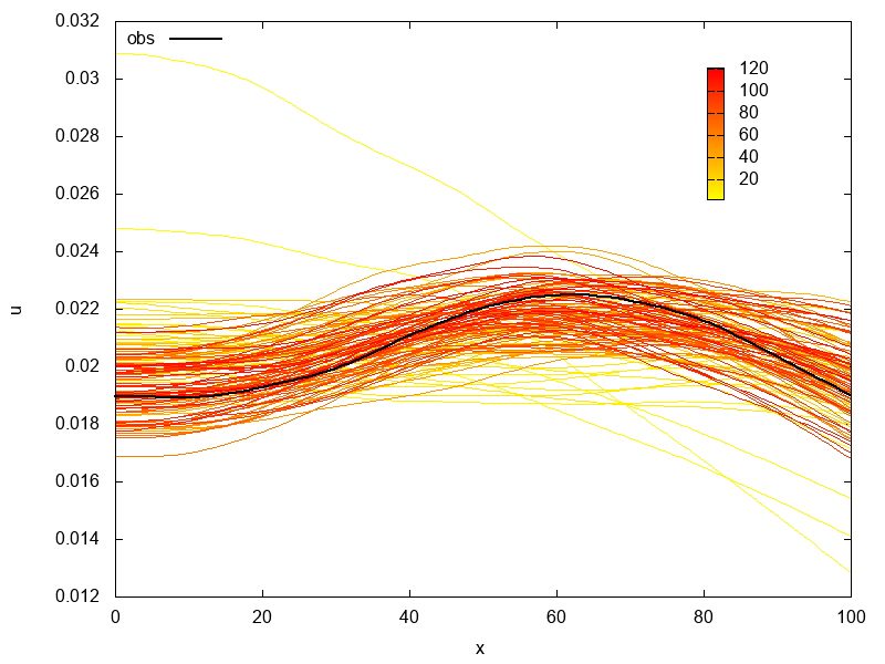
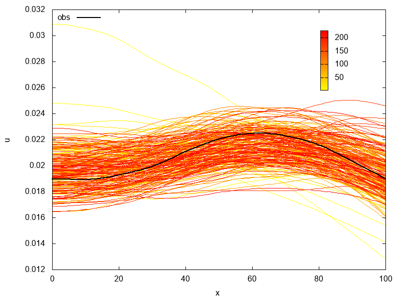
where $F=u(x,t)$, $F^{*}=u^{ms}(x,t)$ where $t=T_{max}$ (final time) and $x\in\partial\Omega_{surf}$ ($\partial\Omega_{surf}$ is the top boundary of the domain). As observation data, we take solution that presented in Figure 13 and 14. We observe that if we take a sufficient number of multiscale basis, we can obtain a good correlation between these two characteristics. From this perspective we will use in our calculations $M_{+}=2$ in MCMC algorithm which have $DOF_{c}=847$ for 2D problem ($M_{p}=3$ and $M_{u}=4$) and $DOF_{c}=1728$ for 3D problem ($M_{p}=3$ and $M_{u}=5$). Fine grid system size is $DOF_{f}=30603$ for two-dimensional problem and $DOF_{f}=37044$ for three-dimensional problem. The random heterogeneity is represented using Karhunen-Loéve expansion. In MCMC iterations, the heterogeneous porosity field is generated using $L=200$ basis functions ($Y_{L}(x,\theta)$) with exponential covariance ($l_{x}=l_{y}=l_{z}=0.2$ and $\sigma_{R}^{2}=2$). Form of $\phi$, $k$ and $E$ are presented in 16, 17 and 18 with $a=40$, $b=0.1$. In numerical simulation, we pick a some realization of the random field $\theta_{ref}$ and use corresponded solution as observation data (see first columns of Figures 13 and 14).

(a) Single-stage MCMC

(b) Two-stage MCMC, $M_{+}=2$

(c) Two-stage MCMC, $M_{+}=4$

Figure 9: Two - dimensional problem with $\sigma_{f}=0.02$. Random walk samples with $\delta=0.5$. First row: accepted $u_{obs}$ on surface boundary. Second row: $E^{*}(\theta)$ (green color) and $E(\theta)$(blue color) in each MCMC iteration. (a) Single-stage MCMC (34 accepted). (b) Two-stage MCMC with $\beta=2$ and $M_{+}=2$ (31 accepted and 69 passed first stage). (b) Two-stage MCMC with $\beta=2$ and $M_{+}=4$ (46 accepted and 68 passed first stage).

Figure 10: Three - dimensional problem with $M_{+}=2$. Two-stage MCMC with $\sigma_{f}=0.02$ and $\beta=2$. Random walk samples with $\delta=0.5$. First row: accepted $u_{obs}$ on surface boundary. Second row: $E^{*}(\theta)$ (green color) and $E(\theta)$(blue color) in each MCMC iteration. 29 accepted and 141 passed the first stage.

(a) Two-stage MCMC, $\sigma_{f}=0.01$

(b) Two-stage MCMC, $\sigma_{f}=0.04$

(c) Two-stage MCMC, $\sigma_{f}=0.06$

Figure 11: Two - dimensional problem with $M_{+}=2$. Two-stage MCMC with $\beta=2$ for different $\sigma_{f}=0.01,0.04,0.06$. Random walk samples with $\delta=0.5$. First row: accepted $u_{obs}$ on surface boundary. Second row: $E^{*}(\theta)$ (green color) and $E(\theta)$(blue color) in each MCMC iteration. (a) $\sigma_{f}=0.01$ (14 accepted and 50 passed first stage). (b) $\sigma_{f}=0.04$ (121 accepted and 212 passed first stage). (c) $\sigma_{f}=0.06$ (226 accepted and 336 passed first stage).

(a) $\sigma_{f}$

(b) $\beta$

(c) $\delta$

Figure 12: Number of accepted and number of passed first stage. Two - dimensional problem. Two-stage MCMC with $M_{+}=2$. (a) $\delta=0.5$, $\sigma_{f}=0.02$, $\beta=1,2,4,6$ and $8$. (b) $\delta=0.5$, $\beta=2$, $\sigma_{f}=0.01,0.02,0.04$ and $0.06$. (c) $\beta=2$, $\sigma_{f}=0.02$, $\delta=0,25,0.5$ and $1.0$.

Figure 13: Reference solution and solutions for accepted random fields for two - dimensional problem (from left to right). Two-stage MCMC with $\sigma_{f}=0.02$, $\beta=2$ and $M_{+}=2$. Random walk samples with $\delta=0.5$. 31 accepted and 69 passed the first stage. First row: permeability, $k$. Second row: elastic modulus, $E$. Third row: pressure, $p$. Fourth row: displacement, $u_{m}$.

Figure 14: Reference solution and solutions for accepted random fields for three - dimensional problem (from left to right). Two-stage MCMC with $\sigma_{f}=0.02$, $\beta=2$ and $M_{+}=2$. Random walk samples with $\delta=0.5$. 29 accepted and 141 passed the first stage. First row: permeability, $k$. Second row: elastic modulus, $E$. Third row: pressure, $p$. Fourth row: displacement, $u_{m}$.

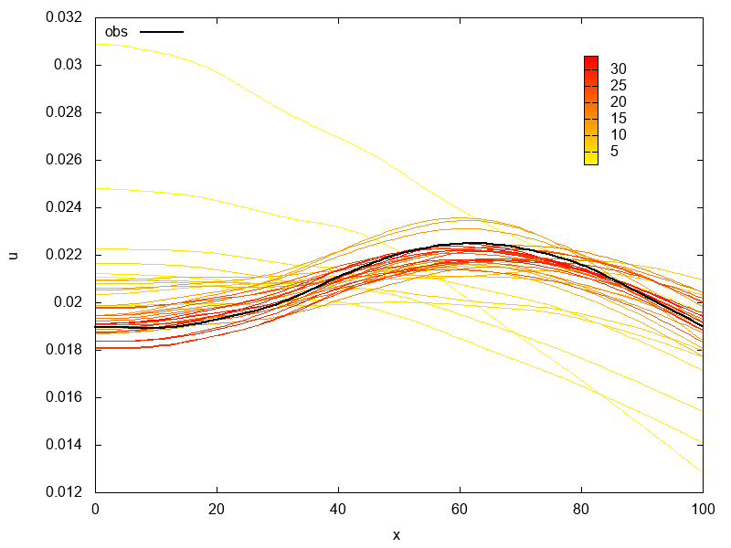
Next, we present results for MCMC algorithms with $\sigma_{c}^{2}=\beta\cdot\,\sigma_{f}^{2}$. We test 1000 random fields proposals and use a random walk sampler for transitional probability distribution

$$q(\theta|\theta_{n})=\theta_{n}+\delta\cdot r,$$

where $r$ is a Gaussian random variable with zero mean and variance 1. We use relative difference between observation data and proposed solution form (26) with $F=u(x,t)$, $F^{*}=u^{ms}(x,t)$ where $t=T_{max}$ (final time) and $x\in\partial\Omega_{surf}$ ($\partial\Omega_{surf}$ is the top boundary of the domain).

We consider the influence of the following parameters on the results and perform the following tests:

• Single-stage and two-stage MCMC method with $M_{+}=2$ and $4$ for 2D problem.

• Two-stage MCMC for three-dimensional test problem with $M_{+}=2$.

• Influence of the $\beta$, $\sigma_{f}$ and $\delta$ to the results of the two-stage MCMC method.

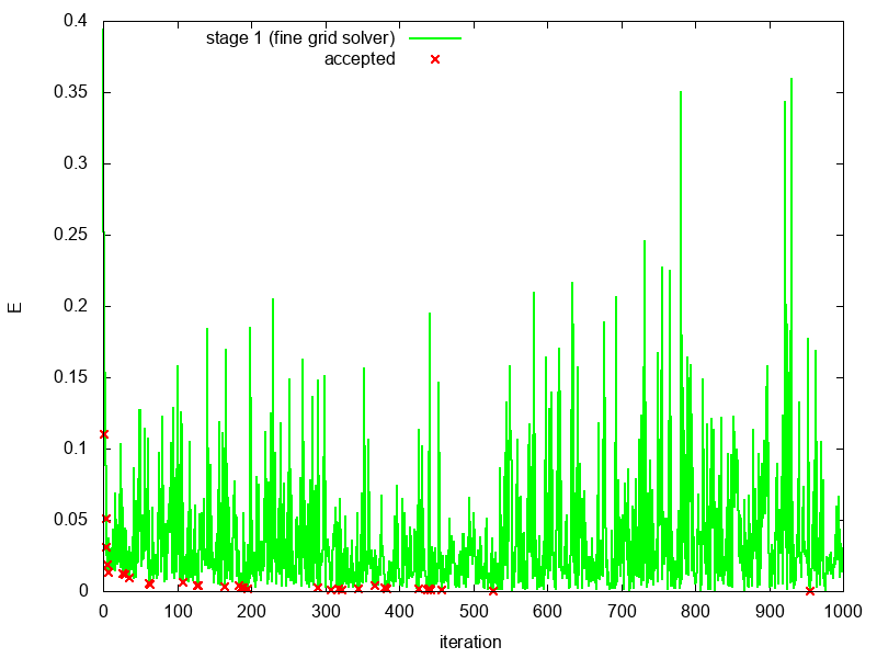
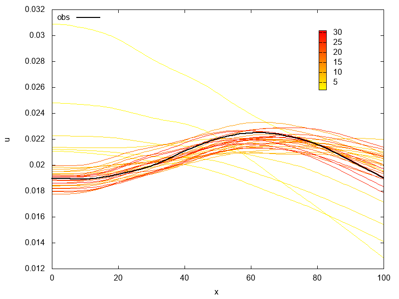
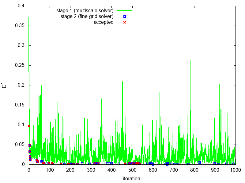
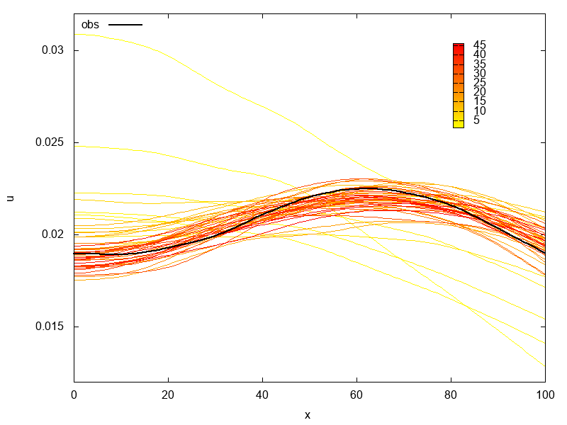
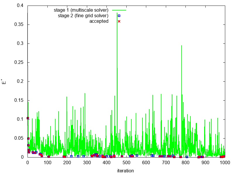
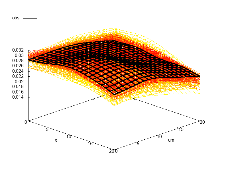
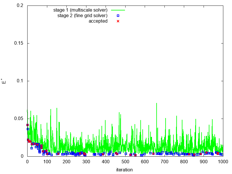
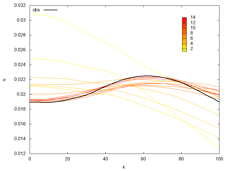
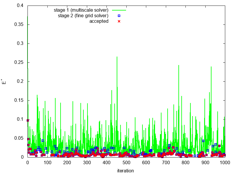
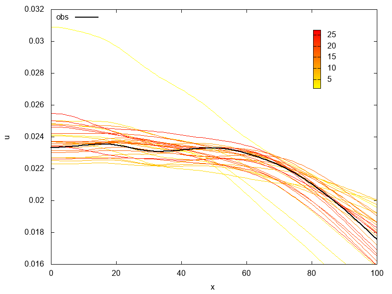
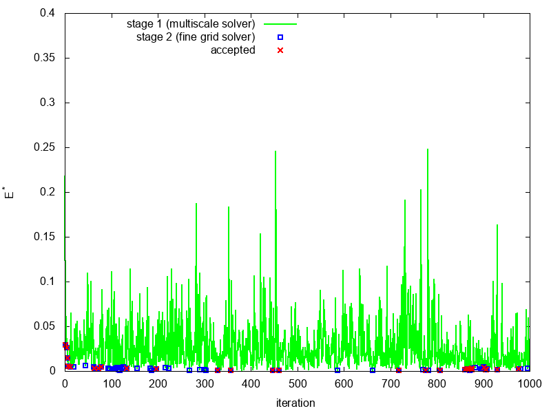
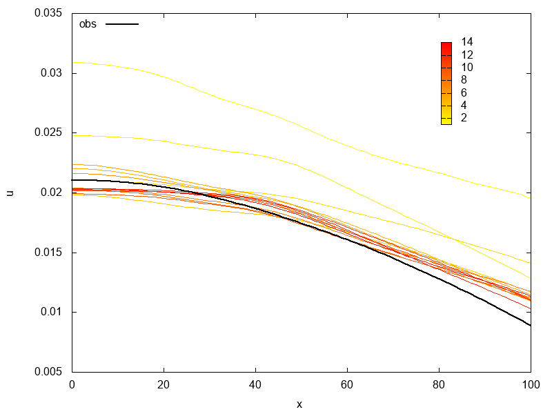
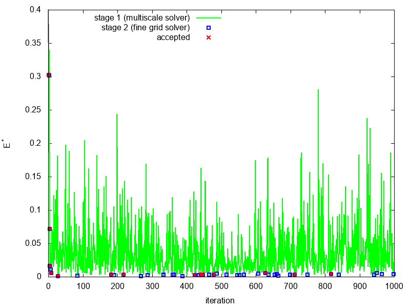
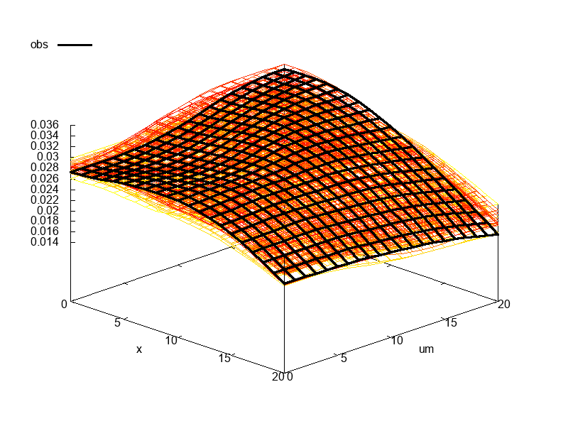
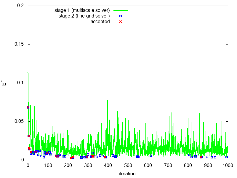
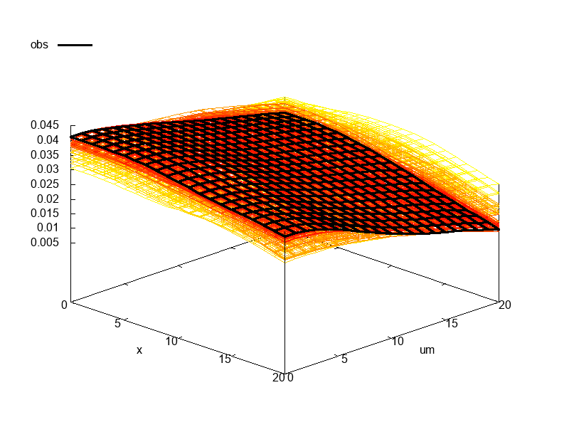
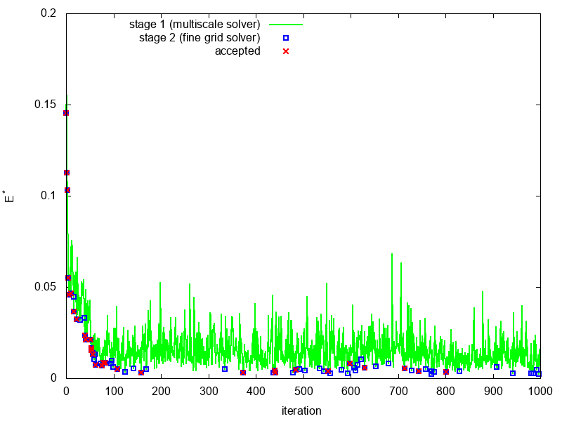
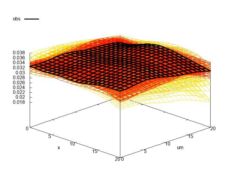
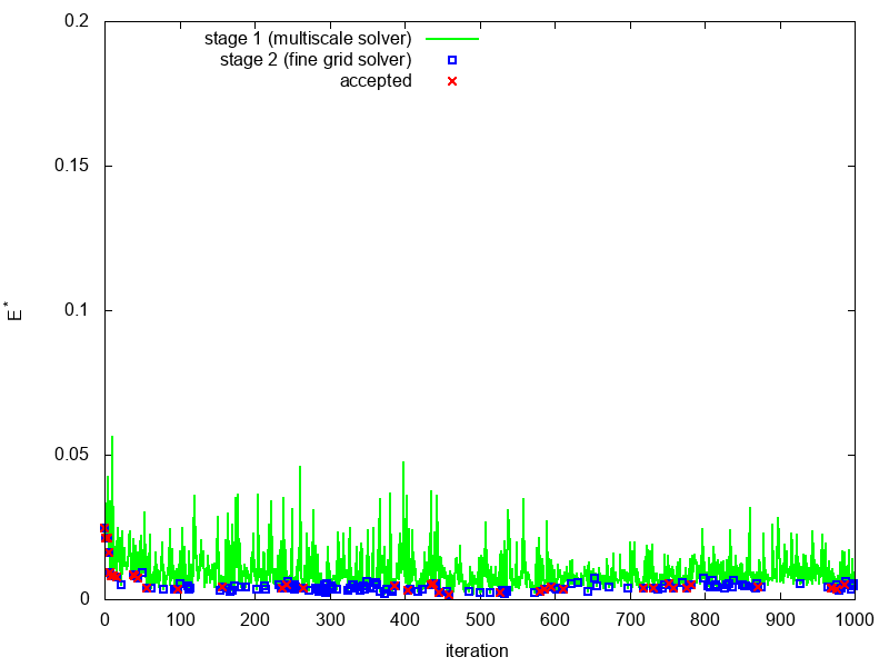
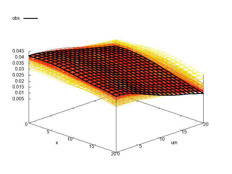
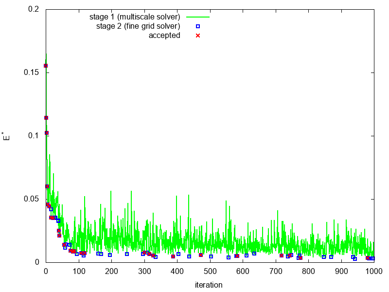
In Figure 9, we present results for single-stage and two-stage MCMC method with $M_{+}=2$ and $4$. In the first row, we depict an accepted $u_{obs}$ on the surface boundary, and on the second row, we present acceptance errors. Results are presented for two - dimensional problem. In MCMC algorithm, we use a random walk sampler with $\delta=0.5$ and set $\sigma_{f}=0.02$. We have 34 accepted fields in a single-stage method. In the two-stage MCMC with $M_{+}=2$ we have 31 accepted and 69 passed first stage. For $M_{+}=4$, we obtain 46 accepted and 68 passed first stage fields. In the first row of Figure 9, we depicted an accepted $u_{obs}$ on the surface boundary, where with gradient coloring from yellow to red related to the number of accepted fields. We observe a convergence of the method from second row, where we depicted relative differences between observation data and the proposed solution. Here $E^{*}(\theta)$ is shown in green color for multiscale solver (fist stage) and $E(\theta)$is shown in blue color for $\theta$ that passed the first stage and calculated using fine grid solver.

In Figure 13, we present examples of accepted permeabilities with a reference solution that we used to calculate observation data (two-dimensional problem). 2D results are shown for two-stage MCMC algorithm with $\sigma_{f}=0.02$, $\beta=2$, $M_{+}=2$ and random walk sampler with $\delta=0.5$. On the first and second rows, we depict permeability and elastic modulus, $k$ and $E$. Pressure and magnitude of the displacements are depicted in the third and fourth rows. In Figures 10 and 14, we present results for three-dimensional case. Results are presented for the two-stage MCMC algorithm with $\sigma_{f}=0.02$, $\beta=2$, $M_{+}=2$ and random walk sampler with $\delta=0.5$. For 2D and 3D results with the same parameters, we obtain:

• 2D: we have 31 accepted and 69 passed the first stage.

• 3D: we have 29 accepted and 141 passed the first stage.

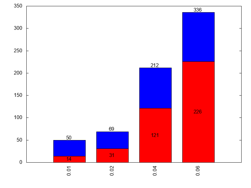
Numerical results for two-stage MCMC with different $\sigma_{f}=0.01,0.04,0.06$ are presented in Figure 11. We perform calculations for $\beta=2$ and random walk sampler with $\delta=0.5$. In Figure 12, we show a histogram with number of accepted and number of passed first stage for two - dimensional problem with $M_{+}=2$ and $\delta=0.5$. In the first picture in Figure 12, we consider $\delta=0.5$, $\beta=2$, $\sigma_{f}=0.01,0.02,0.04$ and $0.06$. We have

• $\sigma_{f}=0.01$: 14 accepted and 50 passed first stage.

• $\sigma_{f}=0.02$: 31 accepted and 69 passed first stage.

• $\sigma_{f}=0.04$: 121 accepted and 212 passed first stage.

• $\sigma_{f}=0.06$: 226 accepted and 336 passed first stage.

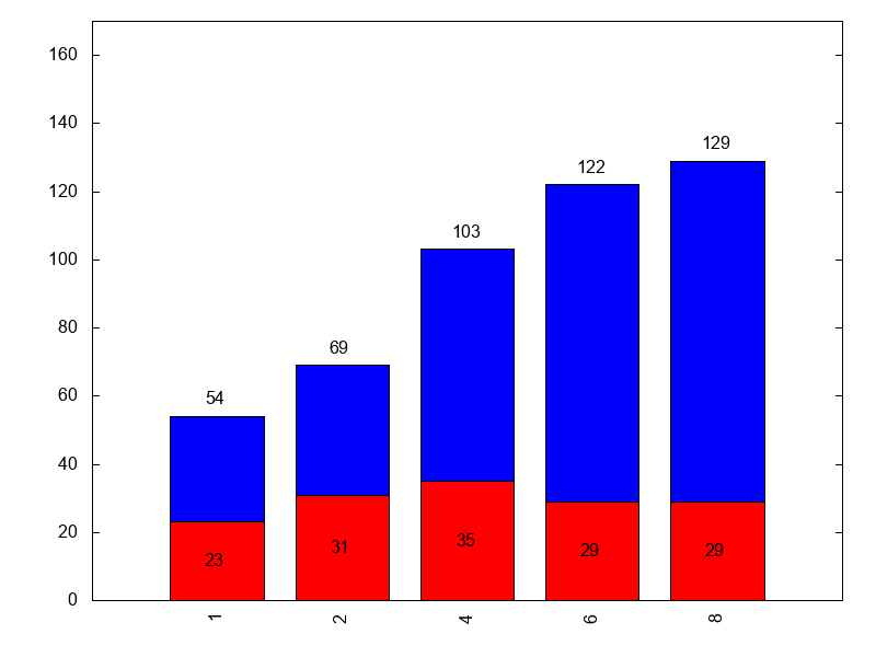
In the second picture, we show results for

$$\sigma_{c}=\beta\cdot\sigma_{f},$$

with $\sigma_{f}=0.02$, $\beta=1,2,4,6$ and $8$. We obtain following results

• $\beta=1$: 23 accepted and 54 passed first stage.

• $\beta=2$: 31 accepted and 69 passed first stage.

• $\beta=4$: 35 accepted and 103 passed first stage.

• $\beta=6$: 29 accepted and 122 passed first stage.

• $\beta=8$: 29 accepted and 129 passed first stage.

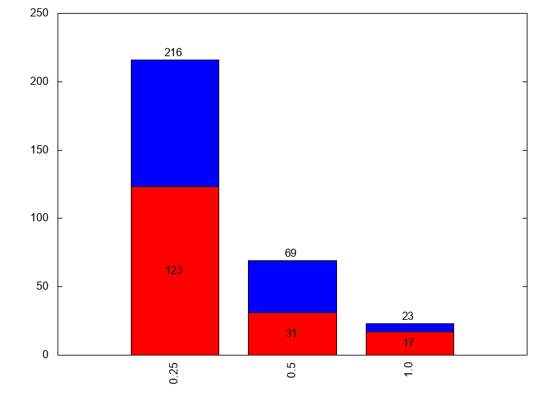
In third picture in Figure 12, we present results for $\beta=2$, $\sigma_{f}=0.02$, $\delta=0,25,0.5$ and $1.0$. We obtain

• $\delta=0.25$: 123 accepted and 216 passed first stage.

• $\delta=0.5$: 31 accepted and 69 passed first stage.

• $\delta=1.0$: 17 accepted and 23 passed first stage.

We see that larger $\beta$ leads to larger acceptance on the first stage. We observe that $\beta=2$ is better to obtain an optimal number of the accepted on the first stage vs the number of the accepted on the fine grid. By increasing the parameter $\sigma_{f}$, we increase the number of the accepted fields by reducing requirements between proposed and observation data differences. The smaller parameter $\delta$ from random walk leads to the larger number of accepted fields, but larger $\delta$ leads to the larger jump in random field generator.

5.3 Preconditioned MCMC using Machine Learning

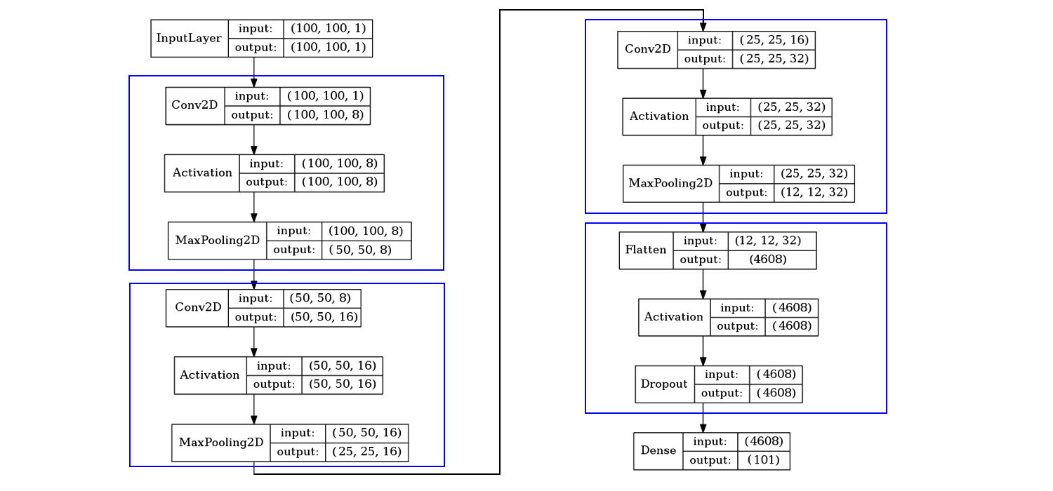
Finally, we consider the preconditioned MCMC method using a machine learning technique (ML). We construct the neural networks for the prediction of the observable data (displacements on the surface boundary). Neural networks are constructed for each direction of displacements separately.

(a) architecture of NN

(b) loss function vs epoch

Figure 15: Two neural networks for the 2D problem. (a) the architecture of neural networks. (b) learning performance, loss function vs epoch. $NN_{x}$ for $x$-displacement with RMSE = 1.887 %, and $NN_{y}$ for $y$-displacement with RMSE = 1.386 % (from left to right).

(a) architecture of NN

(b) loss function vs epoch

Figure 16: Three neural networks for the 3D problem. (a) the architecture of neural networks. (b) learning performance, loss function vs epoch. $NN_{x}$ for $x$-displacement with RMSE = 1.104 %, $NN_{y}$ for $y$-displacement with RMSE = 1.746 %, and $NN_{z}$ for $z$-displacement with RMSE = 1.734 % (from left to right).

	MSE	RMSE (%)	MAE (%)
2D
$NN_{x}$	0.0007	1.8878	1.6719
$NN_{y}$	0.0002	1.3864	1.2660
3D
$NN_{x}$	0.0001	1.1049	0.8978
$NN_{y}$	0.0003	1.7468	1.5461
$NN_{z}$	0.0003	1.7343	1.4264

Table 4: Learning performance of a machine learning algorithms for 2D and 3D formulations.

(a) 2D

(b) 3D

Figure 17: Multiscale method errors for 100 random realizations of heterogeneous filed. Prediction of the machine learning algorithm and multiscale solver with $M_{+}=2,4$. Relative errors in % for displacements on the top boundary.

(a) Case 1 for 2D

(b) Case 2 for 2D

(c) Case 3 for 2D

(d) Case 1 for 3D

(e) Case 2 for 3D

(f) Case 3 for 3D

Figure 18: Cross-plot between ${E(\theta)}$ (fine scale) and ${E^{*}(\theta)}$. Prediction of the machine learning algorithm and multiscale solver with $M_{+}=2,4$. Case 1, 2 and 3 observation data (from left to right). First row: two-dimensional problem. Second row: three-dimensional problem.

(a) Case 1 for 2D (MS)

(b) Case 3 for 2D (MS)

(c) Case 2 for 2D (MS)

Figure 19: Two - dimensional problem with MS preconditioning. Two-stage MCMC with $\sigma_{f}=0.02$ and $\beta=2$. First row: accepted $u_{obs}$ on surface boundary. Second row: $E^{*}(\theta)$ (green color) and $E(\theta)$(blue color) in each MCMC iteration. (a) Case 1. (b) Case 2. (c) Case 3.

(a) Case 1 for 2D (ML)

(b) Case 3 for 2D (ML)

(c) Case 2 for 2D (ML)

Figure 20: Two - dimensional problem with ML preconditioning. Two-stage MCMC with $\sigma_{f}=0.02$ and $\beta=2$. First row: accepted $u_{obs}$ on surface boundary. Second row: $E^{*}(\theta)$ (green color) and $E(\theta)$(blue color) in each MCMC iteration. (a) Case 1. (b) Case 2. (c) Case 3.

(a) Case 1 for 2D (ML)

(b) Case 2 for 2D (ML)

(c) Case 3 for 2D (ML)

Figure 21: Reference field and accepted random fields for three - dimensional problem (from left to right). Two - dimensional problem with ML preconditioning. Two-stage MCMC with $\sigma_{f}=0.02$ and $\beta=2$. (a) $\phi$ for Case 1. (b) $\phi$ for Case 2. (c) $\phi$ for Case 3.

(a) Case 1 for 3D (MS)

(b) Case 3 for 3D (MS)

(c) Case 2 for 3D (MS)

Figure 22: Three - dimensional problem with MS preconditioning. Two-stage MCMC with $\sigma_{f}=0.02$ and $\beta=2$. First row: accepted $u_{obs}$ on surface boundary. Second row: $E^{*}(\theta)$ (green color) and $E(\theta)$(blue color) in each MCMC iteration. (a) Case 1. (b) Case 2. (c) Case 3.

(a) Case 1 for 3D (ML)

(b) Case 3 for 3D (ML)

(c) Case 2 for 3D (ML)

Figure 23: Three - dimensional problem with ML preconditioning. Two-stage MCMC with $\sigma_{f}=0.02$ and $\beta=2$. First row: accepted $u_{obs}$ on surface boundary. Second row: $E^{*}(\theta)$ (green color) and $E(\theta)$(blue color) in each MCMC iteration. (a) Case 1. (b) Case 2. (c) Case 3.

(a) Case 1 for 3D (ML)

(b) Case 2 for 3D (ML)

(c) Case 3 for 3D (ML)

Figure 24: Reference field and accepted random fields for three - dimensional problem (from left to right). Three - dimensional problem with ML preconditioning. Two-stage MCMC with $\sigma_{f}=0.02$ and $\beta=2$. (a) $\phi$ for Case 1. (b) $\phi$ for Case 2. (c) $\phi$ for Case 3.

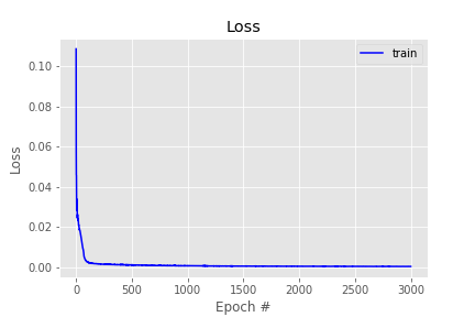
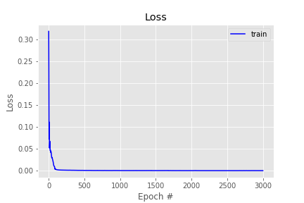
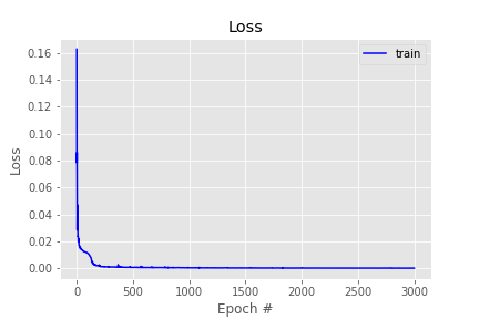
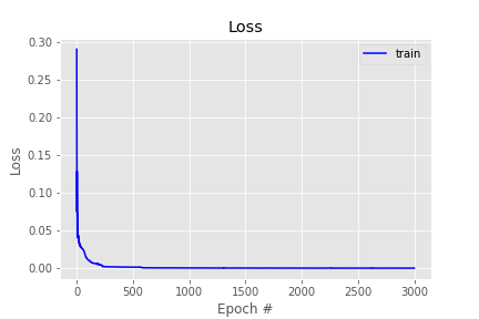
The architectures of the neural networks are presented in Figures 15 and 16 for 2D and 3D problems, respectively. In training process, we perform 3000 epochs using Adam optimizer with learning rate $\epsilon=0.001$. For accelerating the training process of the CNN, we use GPU (GTX 1800 Ti). We use $3^{d}$ convolutions and $2^{d}$ maxpooling layers with RELU activation for $d=2,3$. We have several layers of convolutions with several final fully connected layers. We use dropout with rate 10 % in order to prevent over-fitting. As a loss function, we use a mean square error (MSE). Convergence of the loss function presented in Figures 15 and 16, where we plot the MSE loss function vs epoch number.

For error calculation, we use mean square errors, relative mean absolute and relative root mean square errors

$$MSE=\sum_{i}|Q_{i}-\tilde{Q}_{i}|^{2},\quad RMSE=\sqrt{\frac{\sum_{i}|Q_{i}-\tilde{Q}_{i}|^{2}}{\sum_{i}|Q_{i}|^{2}}},\quad MAE=\frac{\sum_{i}|Q_{i}-\tilde{Q}_{i}|}{\sum_{i}|Q_{i}|},$$

where $Q_{i}$ and $\tilde{Q}_{i}$ denotes reference and predicted values for sample $X_{i}$. Learning performance for neural networks are presented in Tables 4 for two and three - dimensional problems. We observe good convergence of the relative errors with $\approx 1\%$ of RMSE.

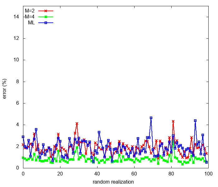
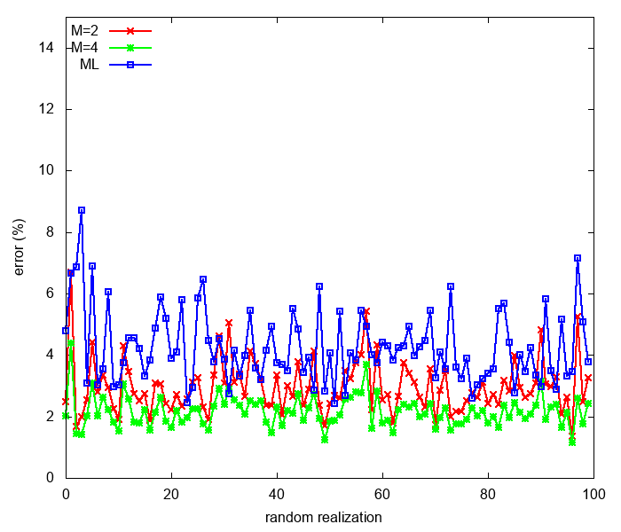
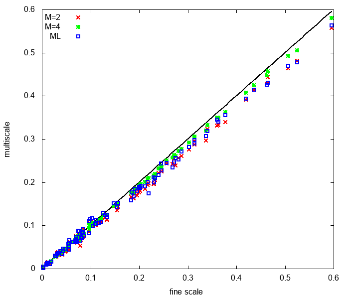
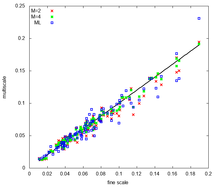
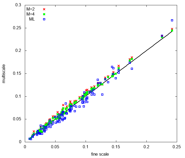
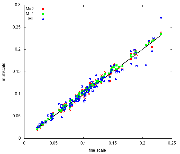
In Figure 18, we present parity plots comparing reference values against predicted using trained neural networks for Case 1, 2 and 3. Cross plot demonstrate correlation between ${E^{*}(\theta)}$ and ${E(\theta)}$ for 100 realizations of random fields for three cases in 2D and 3D formulations. In Figure 17, we present a relative errors for displacements on the top boundary. We compare prediction using reference fine grid values of the displacements. We observe sufficiently good errors for predicted values, where we have less than $5\%$ of errors for 2D and less than $10\%$ of errors for 3D. Later, we will discuss the computational efficiency of the machine learning algorithms compared with direct forward calculations and preconditioning using multiscale solver.

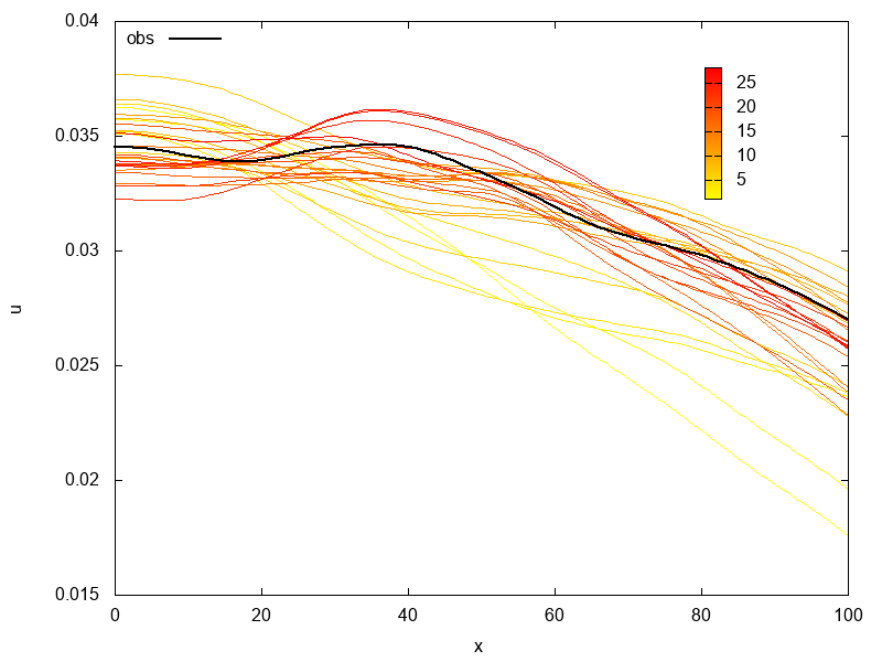
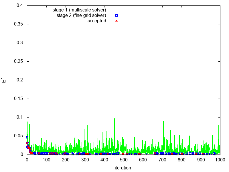
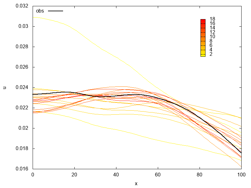
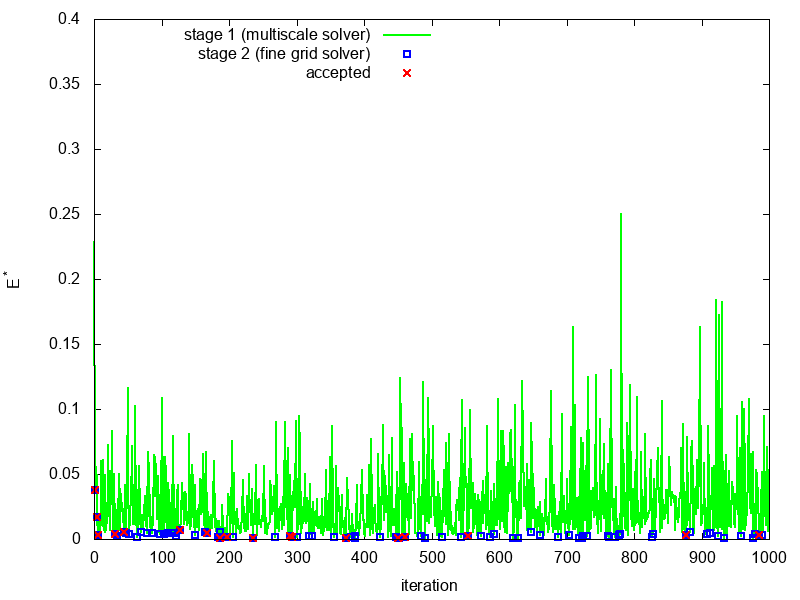
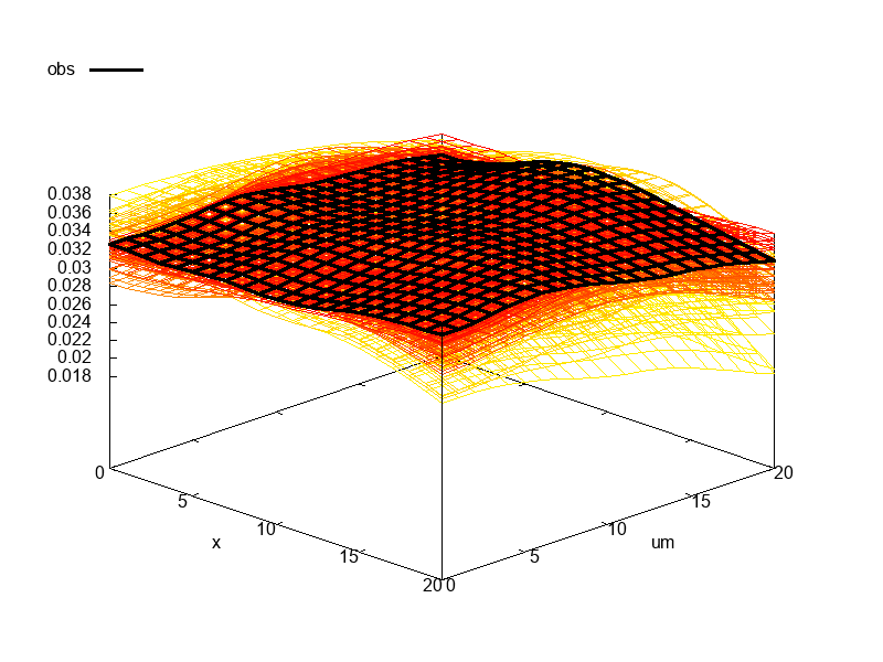
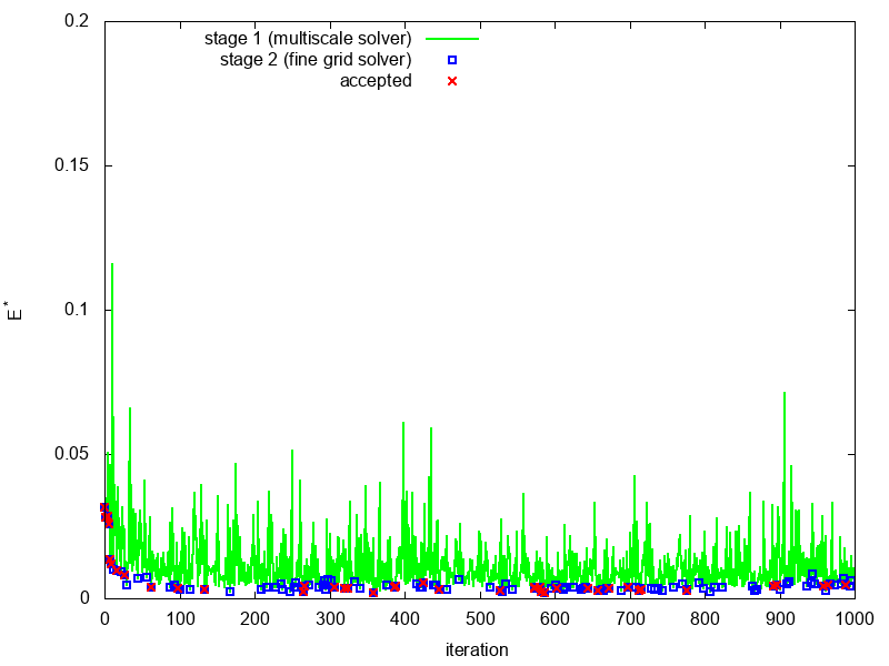
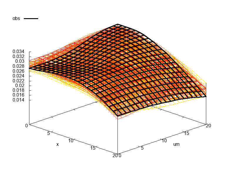
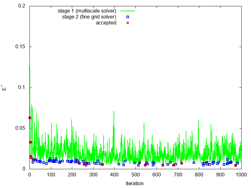
Next, we consider numerical results for the two-stage MCMC method with machine learning technique (ML) and multiscale solver (MS). In Figures 19 and 20, we present results two-dimensional problem for Case 1, 2 and 3 (see Section 5.1). In the first row, we depict an accepted $u_{obs}$ on surface boundary and on the second row, we present an acceptence errors. In MCMC algorithm, we use a random walk sampler with $\delta=0.5$. We use $\sigma_{f}=0.02$ and set $\sigma_{c}=2\cdot\sigma_{f}$.

For MS preconditioning, we have

• Case 1 with 47 accepted and 105 passed first stage.

• Case 2 with 27 accepted and 62 passed first stage.

• Case 3 with 25 accepted and 72 passed first stage.

For ML preconditioning, we have

• Case 1 with 28 accepted and 132 passed first stage.

• Case 2 with 18 accepted and 81 passed first stage.

• Case 3 with 14 accepted and 45 passed first stage.

The results for three-dimensional problem are presented in Figures 22 and 23 for Case 1, 2 and 3 (see Section 5.1).

For MS preconditioning, we have

• Case 1 with 16 accepted and 67 passed first stage.

• Case 2 with 30 accepted and 71 passed first stage.

• Case 3 with 40 accepted and 124 passed first stage.

For ML preconditioning, we have

• Case 1 with 17 accepted and 89 passed first stage.

• Case 2 with 26 accepted and 63 passed first stage.

• Case 3 with 39 accepted and 159 passed first stage.

In Figures 21 and 24, we depict an examples of accepted porosities with a reference porosity that we used to calculate observation data. Numerical results are shown for two-stage MCMC algorithm with ML preconditioning for Case 1,2 and 3 in 2D and 3D formulations.

We observe that we can obtain a good acceptance rate with very cheap machine learning-based prediction. The acceptance rate is $N_{accepted}/N_{fine}$, $N_{accepted}$ and $N_{fine}$ are the number of accepted fields and number of expensive fine grid calculations (passed the first stage). For the fast construction of the dataset that used for training, we used a multiscale solver with $M_{+}=2$.

Finally, we discuss the advantage of the proposed algorithm. In the single-stage MCMC method with $N_{iter}$ iterations, time of calculations $T_{F}$ is equal to number of iterations multiply to time of solution of the fine grid system

$$T_{F}=N_{iter}\cdot t_{fine},$$

where $t_{fine}$ is the time of fine grid system solution. Here for 2D system with $DOF_{f}=30603$, we have $t_{fine}=6.2$ seconds and $t_{fine}=158.7$ seconds for 3D problem with $DOF_{f}=37044$ (see Table 3).

For MS preconditioning of the MCMC method, we have

$$T_{MS}=N_{iter}\cdot t_{ms}+N_{fine}\cdot t_{fine},$$

where $t_{ms}$ is the time of coarse grid system solution using GMsFEM and $N_{fine}$ is the number of accepted on the first stage. For $M_{+}=2$, we have $t_{ms}=0.83$ seconds for 2D problem with $DOF_{c}=847$ and $t_{ms}=9.6$ seconds for 3D problem with $DOF_{c}=1728$ (see Table 3). In preconditioned MCMC method, we obtain that $N_{fine}<<N_{iter}$, and therefore, we have a huge reduction in the solution time because the presented multiscale method provides a huge reduction of the system size, but it still takes some time for the solution.

For further reduction of the time, we proposed a machine learning-based technique with a super quick prediction. For ML preconditioning of the MCMC method, we have

$$T_{ML}=N_{iter}\cdot t_{ml}+N_{fine}\cdot t_{fine},$$

where $t_{ml}$ is the time of coarse grid system solution using trained neural networks. Becuase prediction time is very fast i.e. $t_{ml}<<1$ second, therefore

$$T_{ML}=N_{fine}\cdot t_{fine}.$$

6 Conclusion

Simulation of the poroelasticity is difficult due to the complex heterogeneities and uncertainty. In this work, we considered a Two-stage Markov Chain Monte Carlo method for geomechanical subsidence. We presented two techniques for preconditioning: (MS) multiscale method for model order reduction and (ML) machine learning technique. Numerical results are presented for two- and three-dimensional models to show the efficiency of the method as an expedited MCMC sampling method.

Codes used in this manuscript are publicly available on Bitbucket at https://bitbucket.org/vmasha/ms-mcmc.

References

- [1] Martín Abadi, Paul Barham, Jianmin Chen, Zhifeng Chen, Andy Davis, Jeffrey Dean, Matthieu Devin, Sanjay Ghemawat, Geoffrey Irving, Michael Isard, et al. Tensorflow: a system for large-scale machine learning. In OSDI, volume 16, pages 265–283, 2016.
- [2] Robert Altmann, Eric Chung, Roland Maier, Daniel Peterseim, and Sai-Mang Pun. Computational multiscale methods for linear heterogeneous poroelasticity. Journal of Computational Mathematics, 38(1):41–57, 2020.
- [3] Maurice A Biot. General theory of three-dimensional consolidation. Journal of applied physics, 12(2):155–164, 1941.
- [4] Donald L Brown and Maria Vasilyeva. A generalized multiscale finite element method for poroelasticity problems i: linear problems. Journal of Computational and Applied Mathematics, 294:372–388, 2016.
- [5] Donald L Brown and Maria Vasilyeva. A generalized multiscale finite element method for poroelasticity problems ii: Nonlinear coupling. Journal of Computational and Applied Mathematics, 297:132–146, 2016.
- [6] Roland Bürgmann, Paul A Rosen, and Eric J Fielding. Synthetic aperture radar interferometry to measure earth’s surface topography and its deformation. Annual review of earth and planetary sciences, 28(1):169–209, 2000.
- [7] Nicola Castelletto, Sergey Klevtsov, Hadi Hajibeygi, and Hamdi A Tchelepi. Multiscale two-stage solver for biot’s poroelasticity equations in subsurface media. Computational Geosciences, 23(2):207–224, 2019.
- [8] Siddhartha Chib and Edward Greenberg. Understanding the metropolis-hastings algorithm. The american statistician, 49(4):327–335, 1995.
- [9] François Chollet et al. Keras: Deep learning library for theano and tensorflow. URL: https://keras. io/.
- [10] Yalchin Efendiev, Akhil Datta-Gupta, Victor Ginting, Xiang Ma, and Bani Mallick. An efficient two-stage markov chain monte carlo method for dynamic data integration. Water Resources Research, 41(12), 2005.
- [11] Yalchin Efendiev, Thomas Hou, and Wuan Luo. Preconditioning markov chain monte carlo simulations using coarse-scale models. SIAM Journal on Scientific Computing, 28(2):776–803, 2006.
- [12] Yalchin Efendiev and Thomas Y Hou. Multiscale finite element methods: theory and applications, volume 4. Springer Science & Business Media, 2009.
- [13] Geir Evensen. The ensemble kalman filter: Theoretical formulation and practical implementation. Ocean dynamics, 53(4):343–367, 2003.
- [14] Shubin Fu, Robert Altmann, Eric T Chung, Roland Maier, Daniel Peterseim, and Sai-Mang Pun. Computational multiscale methods for linear poroelasticity with high contrast. Journal of Computational Physics, 395:286–297, 2019.
- [15] Victor Ginting, Felipe Pereira, Michael Presho, and Shaochang Wo. Application of the two-stage markov chain monte carlo method for characterization of fractured reservoirs using a surrogate flow model. Computational Geosciences, 15(4):691, 2011.
- [16] Ramon F Hanssen. Radar interferometry: data interpretation and error analysis, volume 2. Springer Science & Business Media, 2001.
- [17] Jiachuan He, Steven A Mattis, Troy D Butler, and Clint N Dawson. Data-driven uncertainty quantification for predictive flow and transport modeling using support vector machines. Computational Geosciences, 23(4):631–645, 2019.
- [18] Alex Krizhevsky, Ilya Sutskever, and Geoffrey E Hinton. Imagenet classification with deep convolutional neural networks. In Advances in neural information processing systems, pages 1097–1105, 2012.
- [19] Prashant Kumar, Carmen Rodrigo, Francisco J Gaspar, and Cornelis W Oosterlee. A parametric acceleration of multilevel monte carlo convergence for nonlinear variably saturated flow. Computational Geosciences, 24(1):311–331, 2020.
- [20] Yann LeCun, Yoshua Bengio, and Geoffrey Hinton. Deep learning. nature, 521(7553):436, 2015.
- [21] Anders Logg, Kent-Andre Mardal, and Garth Wells. Automated solution of differential equations by the finite element method: The FEniCS book, volume 84. Springer Science & Business Media, 2012.
- [22] Xianlin Ma, Mishal Al-Harbi, Akhil Datta-Gupta, Yalchin Efendiev, et al. An efficient two-stage sampling method for uncertainty quantification in history matching geological models. SPE Journal, 13(01):77–87, 2008.
- [23] Didier Massonnet and Kurt L Feigl. Radar interferometry and its application to changes in the earth’s surface. Reviews of geophysics, 36(4):441–500, 1998.
- [24] Andro Mikelić and Mary F Wheeler. Convergence of iterative coupling for coupled flow and geomechanics. Computational Geosciences, 17(3):455–461, 2013.
- [25] Susan E Minkoff, C Mike Stone, Steve Bryant, Malgorzata Peszynska, and Mary F Wheeler. Coupled fluid flow and geomechanical deformation modeling. Journal of Petroleum Science and Engineering, 38(1-2):37–56, 2003.
- [26] RF Mitchell. A mechanical model for permafrost thaw subsidence. 1977.
- [27] Menel Rahrah and Fred Vermolen. A moving finite element framework for fast infiltration in nonlinear poroelastic media. Computational Geosciences: modeling, simulation and data analysis, 2020.
- [28] Alessio Rucci, DW Vasco, and Fabrizio Novali. Monitoring the geologic storage of carbon dioxide using multicomponent sar interferometry. Geophysical Journal International, 193(1):197–208, 2013.
- [29] Colin M Sayers and Peter MTM Schutjens. An introduction to reservoir geomechanics. The Leading Edge, 26(5):597–601, 2007.
- [30] Antonin Settari, FM Mourits, et al. A coupled reservoir and geomechanical simulation system. Spe Journal, 3(03):219–226, 1998.
- [31] Antonin Settari, Dale A Walters, et al. Advances in coupled geomechanical and reservoir modeling with applications to reservoir compaction. Spe Journal, 6(03):334–342, 2001.
- [32] Irina Sokolova, Muhammad Gusti Bastisya, and Hadi Hajibeygi. Multiscale finite volume method for finite-volume-based simulation of poroelasticity. Journal of Computational Physics, 379:309–324, 2019.
- [33] Aleksei Tyrylgin, Maria Vasilyeva, Denis Spiridonov, and Eric T Chung. Generalized multiscale finite element method for the poroelasticity problem in multicontinuum media. Journal of Computational and Applied Mathematics, 374:112783, 2020.
- [34] DW Vasco, Alessio Rucci, Alessandro Ferretti, Fabrizio Novali, RC Bissell, PS Ringrose, AS Mathieson, and IW Wright. Satellite-based measurements of surface deformation reveal fluid flow associated with the geological storage of carbon dioxide. Geophysical Research Letters, 37(3), 2010.
- [35] Maria Vasilyeva, Eric T Chung, Yalchin Efendiev, and Jihoon Kim. Constrained energy minimization based upscaling for coupled flow and mechanics. Journal of Computational Physics, 376:660–674, 2019.
- [36] Maria Vasilyeva, Wing T Leung, Eric T Chung, Yalchin Efendiev, and Mary Wheeler. Learning macroscopic parameters in nonlinear multiscale simulations using nonlocal multicontinua upscaling techniques. Journal of Computational Physics, page 109323, 2020.
- [37] Maria Vasilyeva and Aleksey Tyrylgin. Machine learning for accelerating effective property prediction for poroelasticity problem in stochastic media. arXiv preprint arXiv:1810.01586, 2018.
- [38] Daegil Yang. A Simulator with numerical upscaling for the analysis of coupled multiphase flow and geomechanics in heterogeneous and deformable porous and fractured media. PhD thesis, 2013.
- [39] Jichao Yin, Han-Young Park, Akhil Datta-Gupta, Michael J King, and Manoj K Choudhary. A hierarchical streamline-assisted history matching approach with global and local parameter updates. Journal of Petroleum Science and Engineering, 80(1):116–130, 2011.
- [40] Mark D Zoback. Reservoir geomechanics. Cambridge University Press, 2010.