Solver-in-the-Loop: Learning from Differentiable Physics to Interact with Iterative PDE-Solvers

Abstract

Finding accurate solutions to partial differential equations (PDEs) is a crucial task in all scientific and engineering disciplines. It has recently been shown that machine learning methods can improve the solution accuracy by correcting for effects not captured by the discretized PDE. We target the problem of reducing numerical errors of iterative PDE solvers and compare different learning approaches for finding complex correction functions. We find that previously used learning approaches are significantly outperformed by methods that integrate the solver into the training loop and thereby allow the model to interact with the PDE during training. This provides the model with realistic input distributions that take previous corrections into account, yielding improvements in accuracy with stable rollouts of several hundred recurrent evaluation steps and surpassing even tailored supervised variants. We highlight the performance of the differentiable physics networks for a wide variety of PDEs, from non-linear advection-diffusion systems to three-dimensional Navier-Stokes flows.

Figure 1: A 3D fluid problem (shown in terms of vorticity) for which the regular simulation introduces numerical errors that deteriorate the resolved dynamics (a). Combining the same solver with a learned corrector trained via differentiable physics (b) significantly reduces errors w.r.t. the reference (c).

1 Introduction

Numerical methods are prevalent in science to improve the understanding of our world, with applications ranging from climate modeling [65, 63] over simulating the efficiency of airplane wings [53] to analyzing blood flow in a human body [31]. These applications are extremely costly to compute due to the fine spatial and temporal resolutions required in real-world scenarios. In this context, deep learning methods are receiving strongly growing attention [45, 4, 20] and show promise to account for those components of the solutions that are difficult to resolve or are not well captured by our physical models. Physical models typically come in the form of PDEs and are discretized in order to be processed by computers. This step inevitably introduces numerical errors. Despite a vast amount of work [17, 2] and experimental evaluations [7, 47], analytic descriptions of these errors remain elusive for most real-world applications of simulations.

In our work, we specifically target the numerical errors that arise in the discretization of PDEs. We show that, despite the lack of closed-form descriptions, discretization errors can be seen as functions with regular and repeating structures and, thus, can be learned by neural networks. Once trained, such a network can be evaluated locally to improve the solution of a PDE-solver, i.e., to reduce its numerical error.

The core of most numerical methods contains some form of iterative process – either in the form of repeated updates over time for explicit solvers or even within a single update step for implicit solvers. Hence, we focus on iterative PDE solving algorithms [19]. We show that neural networks can achieve excellent performance if they take the reaction of the solver into account. This interaction is not possible with supervised learning on pre-computed data alone. Even small inference errors of a supervised model can quickly accumulate over time [67, 34], leading to a data distribution that differs from the distribution of the pre-computed data. For supervised learning methods, this causes deteriorated inference at best and solver explosions at worst.

We demonstrate that neural networks can be successfully trained if they can interact with the respective PDE solver during training. To achieve this, we leverage differentiable simulations [1, 68]. Differentiable simulations allow a trained model to autonomously explore and experience the physical environment and receive directed feedback regarding its interactions throughout the solver iterations. Hence, our work fits into the broader context of machine learning as differentiable programming, and we specifically target recurrent interactions of highly non-linear PDEs with deep neural networks. This combination bears particular promise: it improves generalizing capabilities of the trained models by letting the PDE-solver handle large-scale changes to the data distribution such that the learned model can focus on localized structures not captured by the discretization. While physical models generalize very well, learned models often specialize in data distributions seen at training time. However, we will show that, by combining PDE-based solvers with a learned model, we can arrive at hybrid methods that yield improved accuracy while handling solution manifolds with significant amounts of varying physical behavior.

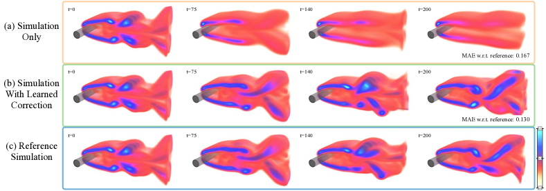
We show the advantages of training via differentiable physics for explicit and implicit solvers applied to a broad class of canonical PDEs. For explicit and semi-implicit solvers, we consider advection-diffusion systems as well as different types of Navier-Stokes variants. We showcase models trained with up to 128 steps of a differentiable simulator and apply our model to complex three-dimensional (3D) flows, as shown in Fig. 1. Additionally, we present a detailed empirical study of different approaches for training neural networks in conjunction with iterative PDE-solvers for recurrent rollouts of several hundred time steps. On the side of implicit solvers, we consider the Poisson problem [42], which is an essential component of many PDE models. Here, our method outperforms existing techniques on predicting initial guesses for a conjugate gradient (CG) solver by receiving feedback from the solver at training time. The source code for this project is available at https://github.com/tum-pbs/Solver-in-the-Loop.

Previous Work

Combining machine learning techniques with PDE models has a long history in machine learning [14, 33, 8]. More recently, deep-learning-based methods were successfully applied to infer stencils of advection-diffusion problems [4], to discover PDE formulations [40, 48, 60], and to analyze families of Poisson equations [41]. While identifying governing equations represents an interesting and challenging task, we instead focus on a general method to improve the solutions of chosen spaces of solutions.

Other studies have investigated the similarities of dynamical systems and deep learning methods [75] and employed conservation laws to learn systems described by Hamiltonian mechanics [20, 13]. Existing studies have also identified discontinuities in finite-difference solutions with deep learning [52] and focused on improving the iterative behavior of linear solvers [28]. So-called Koopman operators likewise represent an interesting opportunity for deep learning algorithms [45, 37]. While these methods replace the PDE-based time integration with a learned version, our models rely on and interact with a PDE-solver that provides a coarse approximation to the problem. Hence, our models always alternate between inference via an artificial neural network (ANN) and a solver step. This distinguishes our work from studies of recurrent ANN architectures [12, 64, 72] as the PDE-solver can introduce significant non-linearities in-between evaluations of the ANN.

We focus on chaotic systems for which fluid flow represents an exciting and challenging problem domain that is highly relevant for industrial applications. Deep learning methods have received significant amounts of attention in this area [36]. For example, both steady [21] and unsteady [45], as well as multi-phase flows [18] have been investigated with deep learning based approaches. Turbulence closure modeling has been an area of particular focus [69, 43, 6]. Additionally, cnns were studied for stochastic sub-grid modeling [70], airfoil flow problems [66, 79], and as part of generative networks to leverage the fast inference of pre-trained models [11, 77, 34]. Other studies have targeted the unsupervised learning of divergence-free corrections [67] or incorporated PDE-based loss functions to represent individual flow solutions via ANNs [49, 60]. In addition to temporal predictions of turbulent flows [44], similar algorithms were more recently also employed for classification problems [24]. However, to the best of our knowledge, the existing methods do not let ANNs interact with solver in a recurrent manner. As we will demonstrate below, this combination yields significant improvements in terms of inference accuracy.

While we focus on Eulerian, i.e., grid-based discretizations, the Lagrangian viewpoint is a popular alternative. While a variety of studies has investigated graph-based simulators, e.g., for rigid-body physics in the context of human reasoning [5, 74, 3] or weather predictions [59], particles are also a popular basis for fluid flow problems [38, 71, 55]. Despite our Eulerian focus, Lagrangian methods could likewise benefit from incorporating differentiable solvers into the training process.

Our work shares the motivation of previous work to use differentiable components at training time [1, 15, 68, 9] and frameworks for differentiable programming [57, 29, 30, 27]. Differentiable physics solvers were proposed for inverse problems in the context of liquids [56], cloth [39], soft robots [29], and molecular dynamics [73]. While these studies typically focus on optimization problems or replace solvers with learned components, we focus on the interaction between the two. Hence, in contrast to previous work, we always rely on a PDE-solver to yield a coarse approximate solution and improve its performance via a trained ANN.

2 Learning to Reduce Numerical Errors

Numerical methods yield approximations of a smooth function ${\bm{u}}$ in a discrete setting and invariably introduce errors. These errors can be measured in terms of the deviation from the exact analytical solution. For discrete simulations of PDEs, they are typically expressed as a function of the truncation, $O(\Delta t^{k})$. Higher-order methods, with large $k$, are preferable but difficult to arrive at in practice. For practical schemes, no closed-form expression exists for truncation errors, and the errors often grow exponentially as solutions are integrated over time. We investigate methods that solve a discretized PDE $\mathcal{P}$ by performing discrete time steps $\Delta t$. Each subsequent step can depend on any number of previous steps, ${\bm{u}}({\bm{x}},t+\Delta t)=\mathcal{P}({\bm{u}}({\bm{x}},t),{\bm{u}}({\bm{x}},t-\Delta t),...)$, where ${\bm{x}}\in\Omega\subseteq\mathbb{R}^{d}$ for the domain $\Omega$ in $d$ dimensions, and $t\in\mathbb{R}^{+}$.

Problem Statement:

We consider two different discrete versions of the same PDE $\mathcal{P}$, with $\mathcal{P}_{R}$ denoting a more accurate discretization with solutions $\mathbf{r}\in\mathscr{R}$ from the reference manifold, and an approximate version $\mathcal{P}_{s}$ with solutions ${\bm{s}}\in\mathscr{S}$ from the source manifold. We consider $\mathbf{r}$ and ${\bm{s}}$ to be states at a certain instance in time, i.e., they represent phase space points, and evolutions over time are given by a trajectory in each solution manifold. As we focus on the discrete setting, a solution over time consists of a reference sequence $\{\mathbf{r}_{t},\mathbf{r}_{t+\Delta t},\cdots,\mathbf{r}_{t+k\Delta t}\}$ in the solution manifold $\mathscr{R}$, and correspondingly, a more coarsely approximated source sequence $\{{\bm{s}}_{t},{\bm{s}}_{t+\Delta t},\cdots,{\bm{s}}_{t+k\Delta t}\}$ exists in the solution manifold $\mathscr{S}$. We also employ a mapping operator $\mathcal{T}$ that transforms a phase space point from one solution manifold to a suitable point in the other manifold, e.g., for the initial conditions of the sequences above, we typically choose ${\bm{s}}_{t}=\mathcal{T}\mathbf{r}_{t}$. We discuss the choice of $\mathcal{T}$ in more detail in the appendix, but in the simplest case, it can be obtained via filtering and re-sampling operations.

By evaluating $\mathcal{P}_{R}$ for $\mathscr{R}$, we can compute the points of the phase space sequences, e.g., $\mathbf{r}_{t+\Delta t}=\mathcal{P}_{R}(\mathbf{r}_{t})$ for an update scheme that only depends on time $t$. Without loss of generality, we assume a fixed $\Delta t$ and denote a state $\mathbf{r}_{t+k\Delta t}$ after $k$ steps of size $\Delta t$ with $\mathbf{r}_{t+k}$. Due to the inherently different numerical approximations, $\mathcal{P}_{s}(\mathcal{T}\mathbf{r}_{t})\neq\mathcal{T}\mathbf{r}_{t+1}$ for the vast majority of states. In chaotic systems, such differences typically grow exponentially over time until they saturate at the level of mean difference between solutions in the two manifolds. We use an $L^{2}$-norm in the following to quantify the deviations, i.e., $\mathcal{L}({\bm{s}}_{t},\mathcal{T}\mathbf{r}_{t})=\|{\bm{s}}_{t}-\mathcal{T}\mathbf{r}_{t}\|_{2}$. Our learning goal is to arrive at a correction operator $\mathcal{C}({\bm{s}})$ such that a solution to which the correction is applied has a lower error than an unmodified solution: $\mathcal{L}(\mathcal{P}_{s}(\mathcal{C}(\mathcal{T}\mathbf{r}_{t_{0}})),\mathcal{T}\mathbf{r}_{t_{1}})<\mathcal{L}(\mathcal{P}_{s}(\mathcal{T}\mathbf{r}_{t_{0}}),\mathcal{T}\mathbf{r}_{t_{1}})$. The correction function $\mathcal{C}({\bm{s}}|\theta)$ is represented as a deep neural network with weights $\theta$ and receives the state ${\bm{s}}$ to infer an additive correction field with the same dimension. To distinguish the original phase states ${\bm{s}}$ from corrected ones, we denote the latter with $\tilde{{\bm{s}}}$, and we use an exponential notation to indicate a recursive application of a function, i.e.,

$${\bm{s}}_{t+n}=\mathcal{P}_{s}(\mathcal{P}_{s}(\cdots\mathcal{P}_{s}(\mathcal{T}\mathbf{r}_{t})\cdots))=\mathcal{P}_{s}^{n}(\mathcal{T}\mathbf{r}_{t})\ .$$ (1)

\begin{overpic}[width=433.62pt]{figs/Manifolds} \put(0.0,2.0){\footnotesize$\mathscr{R}$} \put(36.0,2.0){\footnotesize$\mathscr{S}$} \end{overpic}

Figure 2: Transformed solutions of the reference sequence computed on $\mathscr{R}$ (blue) differ from solutions computed on the source manifold $\mathscr{S}$ (orange). A correction function $\mathcal{C}$ (green) updates the state after each iteration to more closely match the projected reference trajectory on $\mathscr{S}$.

Within this setting, any type of learning method naturally needs to compare states from the source domain with the reference domain in order to bridge the gap between the two solution manifolds. How the evolution in the source manifold at training time is computed, i.e., if and how the corrector interacts with the PDE, has a profound impact on the learning process and the achievable final accuracy. We distinguish three cases: no interaction, a pre-computed form of interaction, and a tight coupling via a differentiable solver in the training loop.

• Non-interacting (NON): The learning task purely uses the unaltered PDE trajectories, i.e., ${\bm{s}}_{t+n}=\mathcal{P}_{s}^{n}(\mathcal{T}\mathbf{r}_{t})$ with $n$ evaluations of $\mathcal{P}_{s}$. These trajectories are fully contained in the source manifold $\mathscr{S}$. Learning from these states means that a model will not see any states that deviate from the original solutions. As a consequence, models trained in this way can exhibit undesirably strong error accumulations over time. This corresponds to learning from the difference between the orange and blue trajectories in Fig. 2, and most commonly applied supervised approaches use this variant.

• Pre-computed interaction (PRE): To let an algorithm learn from states that are closer to those targeted by the correction, i.e., the reference states, a pre-computed or analytic correction is applied. Hence, the training process can make use of phase space states that deviate from those in $\mathscr{S}$, as shown in green in Fig. 2, to improve inference accuracy and stability. This approach can be formulated as ${\bm{s}}_{t+n}=(\mathcal{P}_{s}\mathcal{C}_{\text{pre}})^{n}(\mathcal{T}\mathbf{r}_{t})$ with a pre-computed correction function $\mathcal{C}_{\text{pre}}$. In this setting, the states ${\bm{s}}$ are corrected without employing a neural network, but they should ideally resemble the states achievable via the learned correction later on. As the modified states ${\bm{s}}$ are not influenced by the learning process, the training data can be pre-computed. A correction model $\mathcal{C}({\bm{s}}|\theta)$ is trained via $\tilde{{\bm{s}}}$ that replaces $\mathcal{C}_{\text{pre}}$ at inference time.

• Solver-in-the-loop (SOL): By integrating the learned function into a differentiable physics pipeline, the corrections can interact with the physical system, alter the states, and receive gradients about the future performance of these modifications. The learned function $\mathcal{C}$ now depends on states that are modified and evolved through $\mathcal{P}$ for one or more iterations. A trajectory for $n$ evaluations of $\mathcal{P}_{s}$ is given by $\tilde{{\bm{s}}}_{t+n}=(\mathcal{P}_{s}\mathcal{C})^{n}(\mathcal{T}\mathbf{r}_{t})$, with $\mathcal{C}(\tilde{{\bm{s}}}|\theta)$. The key difference with this approach is that $\mathcal{C}$ is trained via $\tilde{{\bm{s}}}$, i.e., states that were affected by previous evaluations of $\mathcal{C}$, and it affects $\tilde{{\bm{s}}}$ in the following iterations. As for (PRE), this learning setup results in a trajectory like the green one shown in Fig. 2, however, in contrast to before, the learned correction itself influences the evolution of the trajectory, preventing a gap for the data distribution of the inputs.

In addition to these three types of interaction, a second central parameter is the look-ahead trajectory per iteration and mini-batch of the optimizer during learning. A subscript $n$ denotes the number of steps over which the future evolution is recursively evaluated, e.g., SOL_n. The objective function, and hence the quality of the correction, is evaluated with the training goal to minimize $\sum_{i=t}^{t+n}\mathcal{L}({\bm{s}}_{i},\mathbf{r}_{i})$. Below, we will analyze a variety of learning methodologies that are categorized via learning methodology (NON, PRE or SOL) and look-ahead horizon $n$.

3 Experiments

We now provide a summary and discussion of our experiments with the different types of PDE interactions for a selection of physical models. Full details of boundary conditions, parameters, and discretizations of all five PDE scenarios are given in App. B.

3.1 Model Equations and Data Generation

We investigate a diverse set of constrained advection-diffusion models of which the general form is

$$\partial{{\bm{u}}}/\partial{t}=-{\bm{u}}\cdot\nabla{\bm{u}}+\nu\nabla\cdot\nabla{\bm{u}}+\mathbf{g}\quad\text{subject to}\quad{\bm{M}}{\bm{u}}=0,$$ (2)

where ${\bm{u}}$ is the velocity, $\nu$ denotes the diffusion coefficient (i.e., viscosity), and $\mathbf{g}$ denotes external forces. The constraint matrix ${\bm{M}}$ contains an additional set of equality constraints imposed on ${\bm{u}}$. In total, we target four scenarios: pure non-linear advection-diffusion (Burger’s equation), two-dimensional Navier-Stokes flow, Navier-Stokes coupled with a second advection-diffusion equation for a buoyancy-driven flow, and a 3D Navier-Stokes case. Also, we discuss CG solvers in the context of differentiable operators below.

For each of the five scenarios, we implement the non-interacting evaluation (NON) by pre-computing a large-scale data set that captures a representative and non-trivial space of solutions in $\mathscr{S}$. The reference solutions from $\mathscr{R}$ are typically computed with the same numerical method using a finer discretization (4x in our setting, with effective resolutions of $128^{2}$ and higher). The PDEs are parametrized such that the change of discretization leads to substantial differences when integrated over time. For several of the 2D scenarios, we additionally train models with data sets of trajectories that have been corrected with other pre-computated correction functions. For these PRE variants, we use a time-regularized, constrained least-squares corrector [25] to obtain corrected phase state points. For the SOL variants, we employ a differentiable PDE-solver that runs mini-batches of simulations and provides gradients for all operations of the solving process within the deep learning framework. This allows gradients to freely propagate through the PDE-solver and coupled neural networks via automatic differentiation. For $n>1$, i.e., PDE-based look-ahead at training time, the gradients are back-propagated through the solver $n-1$ times, and the difference w.r.t. a pre-computed reference solution is evaluated for all intermediate results.

3.2 Training Procedure

The neural network component $F({\bm{s}}\,|\,\theta)$ of the correction function is realized with a fully convolutional architecture. As our focus lies on the methodology for incorporating PDE models into the training, the architectures are intentionally kept simple. However, they were chosen to yield high accuracy across all variants. Our networks typically consist of 10 convolutional layers with 16 features each, interspresed with ReLU activation functions using kernel sizes of $3^{d}$ and $5^{d}$. The networks parameters $\theta$ are optimized with a fixed number of steps with an ADAM optimizer [35] and a learning rate of $10^{-4}$. For validation, we use data sets generated from the same parameter distribution as the training sets. All results presented in the following use test data sets whose parameter distributions differ from the ones of the training data set.

We quantify the performance of the trained models by computing the mean absolute error between a computed solution and the corresponding projected reference for $n$ consecutive steps of a simulation. We report absolute error values for different models in comparison to an unmodified source trajectory from $\mathscr{S}$. Additionally, relative improvements are given w.r.t. the difference between unmodified source and reference solutions. An improvement by 100% would mean that the projected reference is reproduced perfectly, while negative values indicate that the modified solution deviates more from the reference than the original source trajectory.

\begin{overpic}[height=125.74689pt]{figs/summary-karman} \put(80.0,92.0){\footnotesize(a)} \put(-5.0,66.0){\scriptsize\rotatebox{90.0}{\makebox[42.06119pt]{Source}}} \put(-5.0,33.0){\scriptsize\rotatebox{90.0}{\makebox[42.06119pt]{Corrected}}} \put(-5.0,0.0){\scriptsize\rotatebox{90.0}{\makebox[42.06119pt]{Reference}}} \end{overpic}\begin{overpic}[height=41.6245pt]{figs/summary-legend-karman}\end{overpic}

\begin{overpic}[height=125.74689pt]{figs/summary-smoke} \put(92.0,75.0){\footnotesize{\color[rgb]{1,1,1}(b)}} \end{overpic}\begin{overpic}[height=41.6245pt]{figs/summary-legend-buoy}\end{overpic}

\begin{overpic}[height=125.74689pt]{figs/summary-burgers} \put(90.0,93.0){\footnotesize{\color[rgb]{0,0,0}(c)}} \end{overpic}\begin{overpic}[height=41.6245pt]{figs/summary-legend-burgers}\end{overpic}

Figure 3: Our PDE scenarios cover a wide range of behavior including (a) vortex shedding, (b) complex buoyancy effects, and (c) advection-diffusion systems. Shown are different time steps (l.t.r.) in terms of vorticity for (a), transported density for (b), and angle of velocity direction for (c).

4 Results

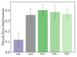
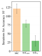
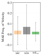
Our experiments show that learned correction functions can achieve substantial gains in accuracy over a regular simulation. When training the correction functions with differentiable physics, this additionally yields further improvements of more than 70% over supervised and pre-computed approaches from previous work. A visual overview of the different tests is given in Fig. 3, and a summary of the full evaluation from the appendix is provided in Fig. 4 and Table 1. In the appendix, we also provide error measurements w.r.t. physical quantities such as kinetic energy and frequency content. The source code of our experiments and analysis will be published upon acceptance.

Unsteady Wake Flow

The PDE scenario for unsteady wake flows represents a standard benchmark case for fluids [50, 45] and involves a continuous inflow with a fixed, circular obstacle, which induces downstream vortex shedding with distinct frequencies depending on the Reynolds number. For coarse discretizations, the approximation errors distort the flow leading to deteriorated motions or suppressed vortex shedding altogether. An example flow configuration is shown in Fig. 3a. In this scenario, the simplest method (NON) yields stable training and a model that already reduces the mean absolute error (MAE) from 0.146 for a regular simulation without correction (SRC) to an MAE of 0.049 when applying the learned correction. The pre-computed correction (PRE) improves on this behavior via its time regularization with an error of 0.031. A SOL₃₂ model trained with a differentiable physics solver for 32 time steps in each iteration of ADAM yields a significantly lower error of 0.013. This means, the numerical errors of the source simulation w.r.t. the reference were reduced by more than a factor of 10. Despite the same architecture and weight count for all three models, the overall performance varies strongly, with the SOL₃₂ version outperforming the simpler variants by 73% and more. An example of the further evaluations provided in the appendix is given in Fig. 4(h).

Buoyancy-driven Flow

We evaluate buoyancy-driven flows as a scenario with increased complexity. In addition to an incompressible fluid, a second, non-uniform marker quantity is advected with the flow that exerts a buoyancy force. This coupled system of equations leads to interesting and complex swirling behavior over time. We additionally use this setup to highlight that the reference solutions can be obtained with different discretization schemes. We use a higher-order advection scheme in addition to a 4$\times$ finer spatial discretization to compute the reference data.

Interestingly, the correction functions benefit from particularly long rollouts at training time in this scenario. Models with simple pre-computed or unaltered trajectories yield mean errors of 1.37 and 1.07 compared to an error of 1.59 for the source simulation, respectively. Instead, a model trained with differentiable physics with 128 steps (SOL₁₂₈) successfully reduces the error to 0.62, an improvement of more than 59% compared to the unmodified simulation.

Forced Advection-Diffusion

A third scenario employs Burger’s equation as a physical model. We mimic the setup from previous work [4] to inject energy into the system via a forcing term with a spectrum of sine waves. This forcing prevents the system from dissipating to relatively static and slowly moving configurations. While the PRE and NON versions yield clear improvements, the SOL versions do not significantly outperform the simpler baselines. This illustrates a limitation of long rollouts via differentiable physics: Learned correction functions need to be able to anticipate future behavior to make high-quality corrections. The randomized forcing in this example severely limits the number of future steps that can accurately be predicted given one state. This behavior contrasts with other physical systems without external disturbances, where a single state uniquely determines its evolution. We show in the appendix that the SOL models with an increased number of interaction steps pay off when the external disturbances are absent.

Conjugate Gradient Solver

We turn to iterative solvers for linear systems of equations to illustrate another aspect of learning from differentiable physics: its importance for the propagation of boundary condition effects. As our learning objective, we target the inference of initial guesses for CG solvers [26]. Following previous work [67], we target Poisson problems of the form $\nabla\cdot\nabla p=\nabla\cdot{\bm{u}}$, which arise for projections of a velocity ${\bm{u}}$ to a divergence-free state. Instead of fully relying on an ANN to produce the pressure field $p$, we instead target the learning objective to produce an initial guess, which is improved by a regular CG solver until a given accuracy threshold is reached.

This goal can be reached by directly minimizing the right-hand side term $\nabla\cdot{\bm{u}}$, similar to physics-based loss terms proposed in a variety of studies [49, 60]. Alternatively, we can employ a differentiable CG solver and formulate the learning goal as minimizing the same residual after $n$ steps of the CG solver (similar to the SOL_n models above). While the physics-based loss version reduces the initial divergence more successfully, it fares badly when interacting with the CG solver: compared to the SOL version, it requires 63% more steps to reach a desired accuracy. Inspecting the inferred solutions reveals that the former model leads to comparatively large errors near boundaries, which are small for each grid cell but significantly influence the solution on a large scale. The SOL version immediately receives feedback about this behavior via the differentiable solver iterations. I.e., the differentiable solver provides a look-ahead of how different parts of the solution affect future states. In this way, it can anticipate problems such as those in the vicinity of boundary conditions.

Three-dimensional Fluid Flow

Lastly, we investigate a 3D case of incompressible flow. The overall setup is similar to the unsteady wake flow in two dimensions outlined above, but the third dimension extends the axes of rotation in the fluid from one to three, yielding a very significant increase in complexity. As a result, the flow behind the cylindrical obstacle quickly becomes chaotic and forms partially turbulent eddies, as shown in Fig. 1. This scenario requires significantly larger models to learn a correction function, and the NON version does not manage to stabilize the flow consistently. Instead, the SOL₁₆ version achieves stable rollouts for several hundred time steps and successfully corrects the numerical inaccuracies of the coarse discretization, improving the numerical accuracy of the source (SRC) simulation by more than 22% across a wide range of configurations.

(a) Unsteady wake

(b) Buoyancy-driven

(c) Advection-diffusion

(d) CG solver

(e) 3D wake

(f) Unsteady wake, look-ahead

(g) Buoyancy-driven, look-ahead

(h) Unsteady wake, frequency error

Figure 4: (a)-(e) Numerical approximation error w.r.t. reference solution for unaltered simulations (SRC) and with learned corrections. The models trained with differentiable physics and look-ahead achieve significant gains over the other models. (f,g) Relative improvement over varying look-ahead horizons. (h) A frequency-based evaluation for the unsteady wake flow scenario.

5 Ablations and Discussion

We performed an analysis of the proposed training via differentiable physics to highlight which hyperparameters most strongly influence results. Specifically, we evaluate varying look-ahead horizons, different model architectures, training via perturbations, and pre-computed variants.

Future Look-Ahead

For systems with deterministic behavior, long rollouts via differentiable physics at training time yield significant improvements, as shown in Fig. 4(f) and 4(g). While training with a few (1 to 4) steps yields improvements of up to 40% for the buoyancy-driven flow scenario, this number can be raised significantly by increasing the look-ahead at training time. A performance of more than 54% can be achieved by 64 recurrent solver iterations, while raising the look-ahead to 128 yields average improvements of 60%. Our tests consistently show that, without changing the number of weights or the architecture of a network, the gradients provided by the longer rollout times allow the network to anticipate the behavior of the physical system better and react to it. Throughout our tests, similar performances could not be obtained by other means.

Generalization

The buoyancy scenario also highlights the very good generalizing capabilities of the resulting models. All test simulations were generated with an out-of-distribution parametrization of the initial conditions, leading to substantially different structures, and velocity ranges over time.

Training with Noise

An interesting variant to stabilize physical predictions in the context of Graph Network-based Simulators was proposed by Sanchez et al. [55]. They report that perturbations of input features with noise lead to more stable long-term rollouts. We mimic this setup in our Eulerian setting by perturbing the inputs to the neural networks with $\mathcal{N}(0,\sigma)$ for varying strengths $\sigma$. While a sweet spot with improvements of 34.5% seems to exist around $\sigma=10^{-4}$, the increase in performance is small compared to a model with less perturbations (30.6%), as training with an increased look-ahead for the SOL models gives improvements up to 60.0%.

Training Stability

The physical models we employ introduce a large amount of complexity into the training loop. Especially during the early stages of training, an inferred correction can overly distort the physical state. Performing time integration via the PDE then typically leads to exponential increases of existing oscillations and a diverging calculation. Hence, we found it important to pre-train networks with small look-aheads (we usually use SOL₂ models), and then continue training with longer recurrent iterations for the look-ahead. While this scheme can be applied hierarchically, we saw no specific gains from, e.g., starting a SOL₃₂ training with a SOL₂ model versus a SOL₁₆ model.

Runtime Performance

The training via differentiable physics incurs an increased computational cost at training time, as the PDE model has to be evaluated for $n$ steps for each learning iteration, and the calculation of the gradients is typically of similar complexity as the evaluation of the PDE itself. However, this incurs only moderate costs in our tests. For example, for the buoyancy-driven flow, the training time increases from 0.21 seconds per iteration on average for SOL₂ to 0.42s for SOL₄, and 1.25s for SOL₁₆. The look-ahead additionally provides $n$ times more gradients at training time, and the inference time of the resulting models is not affected. Hence, the training cost can quickly pay off in practical scenarios by yielding more accurate results without any increase in cost at inference time.

Computing solutions with the resulting hybrid method which alternates PDE evaluations and ANN inference also provides benefits in terms of evaluation performance: A pre-trained, fully convolutional CNN has an $\mathcal{O}(n)$ cost for $n$ degrees of freedom, in contrast to many PDE-solvers with a super-linear complexity. For example, a simulation as shown in Fig. 1 involving the trained model took 13.3s on average for 100 time steps, whereas a CPU-based reference simulation required 913.2s. A speed-up of more than 68$\times$.

Table 1: A summary of the quantitative evaluation for the five PDE scenarios. SOL_s denotes a variant with shorter look-ahead compared to SOL. (^∗ For the CG solver scenario, iterations to reach an accuracy of 0.001 are given. Here, SOL_s denotes the physics-based loss version.)

Exp.	Mean absolute error of velocity					Rel. improvement
	SRC	PRE	NON	SOLs	SOL	PRE	NON	SOLs	SOL
Wake Flow	0.146$\pm$0.004	0.031$\pm$0.010	0.049$\pm$0.012	0.041$\pm$0.009	0.013$\pm$0.003	79%	67%	72%	91%
Buoyancy	1.590$\pm$1.033	1.373$\pm$0.985	1.080$\pm$0.658	0.944$\pm$0.614	0.620$\pm$0.390	19%	29%	41%	60%
Adv.-diff.	0.248$\pm$0.019	0.218$\pm$0.017	0.159$\pm$0.015	0.152$\pm$0.015	0.158$\pm$0.017	12%	36%	39%	36%
∗CG Solver	121.6$\pm$13.44	-	-	79.03$\pm$10.02	29.59$\pm$14.83	-	-	35%	76%
3D Wake	0.167$\pm$0.061	-	0.144$\pm$0.074	-	0.130$\pm$0.058	-	14%	-	22%

6 Conclusions

We have demonstrated how to achieve significant reductions of numerical errors in PDE-solvers by training ANNs with long look-ahead rollouts and differentiable physics solvers. The resulting models yield substantially lower errors than models trained with pre-computed data. We have additionally provided a first thorough evaluation of different methodologies for letting PDE-solvers interact with recurrent ANN evaluations.

Identical networks yield significantly better results purely by having the solver in the learning loop. This indicates that the numerical errors have regular structures that can be learned and corrected via learned representations. The resulting networks likewise improve generalization for out-of-distribution samples and provide stable, long-term recurrent predictions. Our results have the potential to enhance learning physical priors for a variety of deep learning tasks. Beyond engineering applications and medical simulations, a particularly interesting application of our approach is weather prediction [51], where a simple differentiable solver could be augmented with a learned correction function to recover the costly predictions of operational forecasting systems.

Overall, we hope that the demonstrated gains in accuracy will help to establish trained neural networks as components in the numerical toolbox of computational science.

Broader Impact

PDE-based models are very commonly used and can be applied to a wide range of applications, including weather and climate, epidemics, civil engineering, manufacturing processes, and medical applications. Our work has the potential to improve how these PDEs are solved. As PDE-solvers have a long history, there is a wide range of established tools, some of which still use COBOL and FORTRAN. Hence, it will not be easy to integrate deep learning methods into the existing solving pipelines, but in the long run, our method could yield solvers that compute more accurate solutions with a given amount of computational resources.

Due to the wide range of applications of PDEs, our methods could also be used in the development of military equipment (machines and weapons) or other harmful systems. However, our method shares this danger with all numerical methods. For the discipline of computational science as a whole, we see more positive aspects when computer simulations become more powerful. Nonetheless, we will encourage users of our method likewise to consider ethical implications when employing PDE-solvers with learning via differentiable physics.

 

Appendix for Solver-in-the-Loop: Learning from Differentiable Physics to Interact with Iterative PDE-Solvers

 

Below, we give additional details regarding the steps and numerical methods employed in each of the interaction variants discussed in the main text. We present details of the simulation setups for the five scenarios and give more detailed results for each case. Lastly, we discuss performance and list details of our neural network architectures.

As our experiments in the main text already demonstrate, deep learning algorithms that can closely interact with a differentiable PDE solver can yield substantially improved performance. This illustrates how crucial it is for deep learning algorithms that co-exist or interact with numerical solvers in a recurrent manner to anticipate shifts in the distributions of input features. We present additional results and show how interactions between PDE solvers and deep neural networks can be formulated. These interactions help to bridge the gap between distribution shifts that exist between different discretizations of a PDE. We will demonstrate that avoiding distribution shifts is essential for a model to infer a correction successfully. In our iterative setting, this, in turn, helps to keep the distributions aligned over the course of many iterations.

Appendix A Correction Functions for PDEs

For completeness, we provide a brief summary of our notation. We consider reference solutions $\mathbf{r}$ of the PDE $\mathcal{P}$ that are contained in the phase space manifold $\mathscr{R}$ with reference trajectories over time denoted by $\{\mathbf{r}_{t},\mathbf{r}_{t+1},\cdots,\mathbf{r}_{t+k}\}$ for $k$ steps of size $\Delta t$. A more coarsely approximated solution of the same problem is denoted by ${\bm{s}}$ in the manifold $\mathscr{S}$ with trajectories $\{{\bm{s}}_{t},{\bm{s}}_{t+1},\cdots,{\bm{s}}_{t+k}\}$. We typically initialize the source state from the reference version via a transfer operator $\mathcal{T}$ with ${\bm{s}}_{t}=\mathcal{T}\mathbf{r}_{t}$ as initial condition. A transfer from source to reference states is denoted by $\mathcal{T}^{T}$.

The learning objective is to find the best possible correction function $\mathcal{C}({\bm{s}}\,|\,\theta)$ given the weights $\theta$ and a network architecture. Without loss of generality, we assume that the correction function is applied additively, i.e., $\tilde{{\bm{s}}}={\bm{s}}+\mathcal{C}({\bm{s}}\,|\,\theta)$, where the tilde in $\tilde{{\bm{s}}}$ indicates the corrected state. A new state is computed in combination with the PDE via $\tilde{{\bm{s}}}_{t+1}=\mathcal{P}_{s}({\bm{s}}_{t})+\mathcal{C}(\mathcal{P}_{s}({\bm{s}}_{t})\,|\,\theta)$ for which we use the short form $(\mathcal{P}_{s}\mathcal{C})({\bm{s}}_{t})$ below. Multiple recurrent evaluations of a function are denoted by $\tilde{{\bm{s}}}_{t+k}=(\mathcal{P}_{s}\mathcal{C})^{k}({\bm{s}}_{t})$ for $k$ steps starting from an unaltered source state ${\bm{s}}_{t}$.

For training neural networks, we use an $L^{2}$-based loss, i.e., $\mathcal{L}(\tilde{{\bm{s}}}_{t},\mathcal{T}\mathbf{r}_{t})=\|\tilde{{\bm{s}}}_{t}-\mathcal{T}\mathbf{r}_{t}\|^{2}$, which is typically evaluated for $n$ steps via $\sum_{i=t}^{t+n}\mathcal{L}(\tilde{{\bm{s}}}_{i},\mathbf{r}_{i})$ in order to find a solution to the minimization problem: $\operatorname*{arg\,min}_{\theta}\sum_{i=t}^{t+n}\mathcal{L}(\tilde{{\bm{s}}}_{i},\mathbf{r}_{i})$.

We consider constrained advection-diffusion PDEs: $\partial{{\bm{u}}}/\partial{t}=-{\bm{u}}\cdot\nabla{\bm{u}}+\nu\nabla\cdot\nabla{\bm{u}}+\mathbf{g}$ subject to ${\bm{M}}{\bm{u}}=0$. Here, ${\bm{u}}$, $\nu$, and $\mathbf{g}$ denote velocity, diffusivity, and external forces, respectively. The constraint matrix ${\bm{M}}$ contains an additional set of equality constraints imposed on ${\bm{u}}$.

A.1 Learning Without Interaction

In the main text, we use learning via non-interacting trajectories as a baseline learning setup. In this case, a model is trained to minimize differences between states ${\bm{s}}$ and $\mathbf{r}$ in a fully supervised manner. These versions are denoted by NON.

Despite its simplicity, different variants of this learning setup can be considered. In the simplest case, we initialize the source simulation from the corresponding reference version, evaluate the PDE once, and then train a model via a large number of such cases. In our notation, this means learning from states computed as ${\bm{s}}_{t+1}=\mathcal{P}_{s}(\mathcal{T}\mathbf{r}_{t})$. This effectively takes into account only a single evaluation of the source PDE, and a model can only learn from numerical differences that build up within this single step. Hence, a variant of this approach is to allow reference and target version to evolve over the course of multiple steps such that the errors in the source states ${\bm{s}}$ show up more clearly with respect to $\mathbf{r}$. Similar to the look-ahead discussed in the main text, we can use ${\bm{s}}_{t+n}=\mathcal{P}_{s}^{n}(\mathcal{T}\mathbf{r}_{t})$ as a training data set. We denote such versions that have no interaction but consider multiple steps of unaltered coarse evolution as NON_n below. Note that the previously discussed NON version could be denoted by NON₁, but we keep the label NON for consistency with the main text in the following.

For all choices of $n$, we obtain the following minimization problem for learning via non-interacting solvers:

$$\operatorname*{arg\,min}_{\theta}\sum_{i=0}^{n}\|{\bm{s}}_{t+i}+\mathcal{C}({\bm{s}}_{t+i}\,|\,\theta)-\mathcal{T}\mathbf{r}_{t+i}\|^{2}.$$ (3)

Another non-interacting variant could be trained by reversing the setup above and initializing reference trajectories from source states, i.e., $\mathbf{r}_{t+n}=\mathcal{P}_{R}^{n}(\mathcal{T}^{T}{\bm{s}}_{t})$. Like before, a model could be trained in a supervised fashion from a data set of ${\bm{s}}$ and $\mathbf{r}$ states computed in this way. However, as the interesting structures that make up the reference solutions typically take very long time spans to form (if they are achievable at all), this variant is clearly sub-optimal. Hence, due to the poor performance of the NON_n versions, we have not included this reversed NON variant in our experiments.

The NON models presented in the main text so far already allow for a first quantification of the problems caused by the distribution shifts of the input features: across the two-dimensional fluid flow cases, the unaltered source simulations deviate by more than 50% in terms of MAE from the corrected simulations. This means that, after applying the corrections, the model receives inputs that strongly differ from those seen at training time. In terms of content of the input feature vectors, the MAE measurements show a change of over 50%. Nonetheless, we expect the model to reconstruct the reference states despite receiving inputs that are significantly different from the inputs seen at the time of training. Not surprisingly, the models only have limited success achieving this goal.

A.2 Pre-computed Interactions

As an improvement over the non-interacting versions above, we consider a class of models learning from data generated via pre-computed interactions, denoted by PRE. The pre-computations have the goal of reducing the gap between source and reference trajectories. The pre-computation changes the source trajectories and thus provides the learning optimization with modified inputs that are closer to the reference at inference time. This scenario is common practice, e.g., for weather predictions, where simulations need to be aligned with real-world measurements, i.e., data assimilation algorithms [32, 62, 76]. As the data set has to be prepared only once, computationally expensive pre-computation is often still feasible as this overhead will not influence the performance at inference time. However, in the context of machine learning, pre-computed corrections can only provide limited improvements as the correction during the pre-computation phase can only partially mimic the behavior of the actual, learned version.

For PRE models, two correction functions are used: one for preparing the training data set denoted by $\mathcal{C}_{\text{pre}}$ and the learned correction $\mathcal{C}$. The training data set is computed as $\tilde{{\bm{s}}}_{t+n}=(\mathcal{P}_{s}\mathcal{C}_{\text{pre}})^{n}(\mathcal{T}\mathbf{r}_{t})$, where $n$ denotes the number of steps for independent simulation trajectories in the source and reference manifolds. Note that, in this context, due to the corrections being applied at the time of data generation, there is hope for longer unrolling periods (i.e., larger $n$) to have a positive effect on the learning outcome (in contrast to the NON_n versions above). At inference time, $\mathcal{C}_{\text{pre}}$ is no longer used, and trajectories are instead computed as $\tilde{{\bm{s}}}_{t+n}=(\mathcal{P}_{s}\mathcal{C})^{n}({\bm{s}}_{t})$, in line with the NON variants. Hence, in total, four versions of a trajectory from a single initial phase space point $\mathbf{r}_{t}$ exist: a source trajectory, a source trajectory corrected by pre-computation via $\mathcal{C}_{\text{pre}}$, a source trajectory corrected by the learned correction function $\mathcal{C}$, and the reference trajectory.

We first describe how to include a pre-computation correction for spatial corrections while taking into account simulation constraints before including the temporal dimension. For both, we adopt a constrained version of best linear unbiased estimates [25], which are widely used for data assimilation.

A.2.1 Pre-computed Spatial Regularization

For a constraint-aware interpolation that can serve as a correction operator, consider two vector spaces $\mathbf{R}\in\mathbb{R}^{\chi}$ and $\mathbf{S}\in\mathbb{R}^{\xi}$ with different dimensionalities $\xi,\chi\in\mathbb{N}$ with $\xi<\chi$. Both vector spaces satisfy the constraint ${\bm{M}}$, i.e., ${\bm{M}}\mathbf{r}=0$ for $\forall\mathbf{r}\in\mathbf{R}$, and ${\bm{M}}\mathbf{s}=0$ for $\forall\mathbf{s}\in\mathbf{S}$. Given a finer vector field $\mathbf{c}_{R}$, e.g., containing the reference solutions, we aim to find the closest vector field $\mathbf{c}_{S}$ ($\in\mathbf{S}$) to $\mathbf{c}_{R}$ ($\in\mathbf{R}$). Consider an interpolation operator ${\bm{W}}$ that introduces new data points within a vector field $\mathbf{c}_{S}$ ($\in\mathbf{S}$), i.e., ${\bm{W}}\mathbf{c}_{S}\in\mathbb{R}^{\chi}$. We, then, strive to minimize the distance between ${\bm{W}}\mathbf{c}_{S}$ and $\mathbf{c}_{R}$ such that $\mathbf{c}_{S}$ can best represent the information of $\mathbf{c}_{R}$ without violating the constraints. Thus, we aim for computing $\mathbf{c}_{S}$ with

$$\operatorname*{arg\,min}_{\mathbf{c}_{S}}||{\bm{W}}\mathbf{c}_{S}-\mathbf{c}_{R}||^{2}\quad\text{subject to}\quad{\bm{M}}\mathbf{c}_{S}=0.$$ (4)

This represents a constrained optimization problem with equality constraints, which we can solve via Lagrange multipliers $\mathbf{\lambda}$ as follows:

$$\Phi=||{\bm{W}}\mathbf{c}_{S}-\mathbf{c}_{R}||^{2}+({\bm{M}}\mathbf{c}_{S})^{\top}\mathbf{\lambda}.$$ (5)

This results in a system of equations:

$$\begin{bmatrix}{\bm{W}}^{\top}{\bm{W}}&-{\bm{M}}\\ -{\bm{M}}^{\top}&0\end{bmatrix}\begin{bmatrix}\mathbf{c}_{S}\\ \mathbf{\lambda}\end{bmatrix}=\begin{bmatrix}{\bm{W}}^{\top}\mathbf{c}_{R}\\ 0\end{bmatrix}.$$ (6)

Using the Schur complement, we can simplify this system to speed up calculations:

$${\bm{M}}^{\top}({\bm{W}}^{\top}{\bm{W}})^{-1}{\bm{M}}\mathbf{\lambda} = {\bm{M}}^{\top}({\bm{W}}^{\top}{\bm{W}})^{-1}{\bm{W}}^{\top}\mathbf{c}_{R},$$ (7)

$$\mathbf{c}_{S} = ({\bm{W}}^{\top}{\bm{W}})^{-1}({\bm{W}}^{\top}\mathbf{c}_{R}-{\bm{M}}\mathbf{\lambda}).$$ (8)

In our setting, given source states ${\bm{s}}$ and reference states $\mathbf{r}$, we can thus compute a correction vector field via $\mathbf{c}_{t}=({\bm{W}}^{\top}{\bm{W}})^{-1}({\bm{W}}^{\top}(\mathbf{r}_{t}-{\bm{W}}{\bm{s}}_{t})-{\bm{M}}\mathbf{\lambda})$, e.g., using ${\bm{M}}=(\nabla\cdot)$ for Navier-Stokes scenarios. In order to train a model $\mathcal{C}({\bm{s}}\,|\,\theta)$ to infer the corrections, we can directly use the pre-computed correction vectors:

$$\operatorname*{arg\,min}_{\theta}\sum_{i=0}^{n}\|\mathbf{c}_{t+i}-\mathcal{C}(\tilde{{\bm{s}}}_{t+i}|\theta)\|^{2}.$$ (9)

We will denote versions using this pre-computation scheme for $\mathcal{C}_{\text{pre}}$ with spatial regularization as PRE${}_{\text{SR}}$.

A.2.2 Pre-computed Spatiotemporal Regularization

The vector fields we target are obtained from a numerical simulation, where the underlying PDE is solved for a finite number of steps from an initial condition. In the context of deep learning, an important aspect to consider is the sensitivity [46] of the targeted function (i.e., the correction) with respect to the data at hand, i.e., in our case, the state of a source simulation. The pre-computation process described in the previous section is typically done on a per-time-step basis, and hence correction vector fields can vary significantly even for smooth changes of the source simulation. That means the correction function can have a very nonlinear and difficult to learn relationship with the observable data in a simulation.

In order to address this difficulty, we include a temporal regularization by limiting the changes over time for each sample point in space. Consequently, we regularize our correction vector fields such that they change smoothly in time by penalizing temporal change of the correction vector field within the Lagrange multiplier framework. We minimize $d\mathbf{c}_{S}/dt$ together with the constrained transfer from fine to coarse discretizations:

$$\operatorname*{arg\,min}_{\mathbf{c}_{S}}\left(||{\bm{W}}\mathbf{c}_{S}-\mathbf{c}_{R}||^{2}+\beta||\frac{d\mathbf{c}_{S}}{dt}||^{2}\right)\quad\text{subject to}\quad{\bm{M}}\mathbf{c}_{S}=0.$$ (10)

Here, $\beta$ is the temporal regularization coefficient. A finite difference approximation of the temporal derivative of the correction field, i.e., $d\mathbf{c}_{S}/dt$, yields the following system of equations:

$$\begin{bmatrix}{\bm{W}}^{\top}{\bm{W}}+\beta\frac{2}{\Delta t}\mathbf{I}&-{\bm{M}}\\ -{\bm{M}}^{\top}&0\end{bmatrix}\begin{bmatrix}\mathbf{c}_{S}\\ \mathbf{\lambda}\end{bmatrix}=\begin{bmatrix}{\bm{W}}^{\top}\mathbf{c}_{R}+\beta\frac{2}{\Delta t}\mathbf{c}_{S}^{t-1}\\ 0\end{bmatrix},$$ (11)

where $\Delta{t}$ is the time step size, $\mathbf{I}$ is the identity matrix, and $\mathbf{c}_{S}^{t-1}$ denotes the correction vector field evaluated at the previous time step. Following Eq. 9, this data is pre-computed and used for training a neural network in a supervised manner. Models trained with data from this spatiotemporal pre-computation as $\mathcal{C}_{\text{pre}}$ are denoted by PRE, and we have used a coefficient of $\beta=1.0$ for all PRE models of our submission.

A.3 Solver-in-the-Loop Interactions via Differentiable Physics

The main goal of training via differentiable physics is to bridge the gap that arises from changes in the input data distribution and directly train with the environment that the learned model is supposed to work with at inference time. Hence, the learning process aims to solve the minimization problem

$$\operatorname*{arg\,min}_{\theta}\sum_{i=0}^{n-1}\|\mathcal{P}_{s}(\tilde{{\bm{s}}}_{t+i})+\mathcal{C}(\mathcal{P}_{s}(\tilde{{\bm{s}}}_{t+i})|\theta)-\mathcal{T}\mathbf{r}_{t+i+1}\|^{2},$$ (12)

where the phase space trajectories are computed via $\tilde{{\bm{s}}}_{t+k}=(\mathcal{P}_{s}\mathcal{C})^{k}(\mathcal{T}\mathbf{r}_{t})$. This formulation illustrates that a cyclic dependency between the corrected states $\tilde{{\bm{s}}}$ and the learned correction function $\mathcal{C}$ exists for the “solver-in-the-loop” interactions of this section. As both the deep neural network for $\mathcal{C}$ and likewise the PDE $\mathcal{P}_{s}$ are potentially highly non-linear operators, the corresponding coupled minimization problem for calculating the weights of $\mathcal{C}$ is challenging. However, our results clearly show that stable optimizations can be achieved in practice and that they lead to very significant improvements of the learned representation.

The recurrent training requires differentiable physics solvers that allow for a back-propagation of gradients through the discretized physical simulation. In this work, we employ a differentiable PDE solver from the open source $\Phi_{\textrm{Flow}}$ library [27]. This solver builds on the automatic differentiation of the underlying machine learning framework to compute analytic derivatives and augments them with custom derivatives where necessary. For example, the pressure correction step of a Navier-Stokes solver is provided with a custom gradient for performance reasons. This setup allows for a straightforward integration of solver functionality into machine learning models and enables end-to-end training in recurrent settings. Although all of our examples use the $\Phi_{\textrm{Flow}}$ solver, we do not leverage any special functionality apart from gradients being provided for all steps of the PDE solve. Hence, our results should carry over to other types of differentiable physics solvers.

It is worth noting that, in the setup discussed so far, the reference solver does not need to be differentiable; i.e., the phase space points in $\mathscr{R}$ could be provided by a black-box approximation without gradients as long as a differentiable solver for the source manifold $\mathscr{S}$ exists. We demonstrate the split setup using an external solver for the buoyancy-driven flows below.

Our implementation directly follows Eq. 12. For each mini-batch, we start with a collection of reference states $\mathbf{r}$ for which recurrent trajectories of $(\mathcal{P}_{s}\mathcal{C})^{n}$ are unrolled for $n$ steps. The loss with respect to corresponding reference states is computed over all intermediate states of the trajectory. Back-propagation, then, unrolls the differences through the sequence of solver steps to update the weights of the neural network that provides the correction function.

Under the assumption that the training process converges, this entirely removes the problem of distribution shift. Once the learned correction $\mathcal{C}$ converges to a steady-state, it is trained with exactly the phase state inputs that are produced at inference time. The MAE of the test data samples again provides a measure of the discrepancies. Compared to the differences of around 50% for non-interacting variants (measured between source states and corrected states), the deviations grow to 75% and above for SOL versions. Nonetheless, even this larger difference in terms of input distributions is unproblematic here as the network receives the modified states at training time. However, we noticed that, during our training runs, the final states typically do not fully converge, but still show smaller oscillations in terms of performance. While this could be prevented via learning-rate decay, we believe the slightly changing states provide robustness similar to dropout or manual injections of noise [55].

While the error accumulates and typically grows over the course of a full trajectory, our key hypothesis here is that a learned approach can nonetheless identify and correct a large part of the error function based on information from a single phase-space input. For the PDEs we consider, a single state uniquely describes its future evolution. We have experimented with additionally providing varying numbers of previous states $\mathbf{s}_{t-k},...,\mathbf{s}_{t-1}$ as input to our model. Our tests have not shown improvements from these additional states and indicate that the components of the error function that are learned with our approach can be reliably inferred from a single state $\mathbf{s}_{t}$.

Appendix B Experiments

To acquire our data sets, we generate a set of simulation sequences with varying initial conditions. These sequences are used for obtaining pairs of source and reference velocity fields for training. The following PDEs typically work with a continuous velocity field ${\bm{u}}$ with $d$ dimensions and components, i.e., ${\bm{u}}({\bm{x}},t):\mathbb{R}^{d}\rightarrow\mathbb{R}^{d}$. For discretized versions below, $d_{i,j}$ will denote the dimensionality of a field such as the velocity with $i\in\{s,r\}$ denoting source/inference manifold and reference manifold, respectively. This yields ${\bm{s}}\in\mathbb{R}^{d\times d_{s,x}\times d_{s,y}\times d_{s,z}}$ and $\mathbf{r}\in\mathbb{R}^{d\times d_{r,x}\times d_{r,y}\times d_{r,z}}$ with domain size $d_{x},d_{y},d_{z}$ for source and reference. Typically, $d_{r,i}>d_{s,i}$ and $d_{z}=1$ for $d=2$. For all PDEs, we use non-dimensional parametrizations as outlined below, and the components of the velocity vector are denoted by $x,y,z$ subscripts, i.e., ${\bm{u}}=(u_{x},u_{y},u_{z})^{T}$ for $d=3$.

The mapping function $\mathcal{T}$ denotes a projection to the source manifold by $\mathcal{T}\mathbf{r}_{t}$, and we assume that the transpose transforms to the reference manifold, i.e., $\mathcal{T}^{T}{\bm{s}}_{t}$. The mapping function is typically neither bijective nor unique, i.e., $\mathcal{T}^{T}\mathcal{T}\mathbf{r}_{t}\neq\mathbf{r}_{t}$, however, within this work, we are primarily concerned with retrieving projected references of the form $\mathcal{T}\mathbf{r}_{t}$. The potential null-space of $\mathcal{T}^{T}$ is an interesting topic for super-resolution approaches [16]. We found that a bi- or tri-linear spatial downsampling from reference to source space is efficient to compute and yields sufficient accuracy for the transfer in our experiments. In order to make comparisons with the source simulations easier, we visualize the projected reference solution, i.e., $\mathcal{T}\mathbf{r}_{t}$, in the following.

B.1 Unsteady Wake Flow in Two Dimensions

For the unsteady wake flow setup, we use the incompressible Navier-Stokes equations for Newtonian fluids:

$$\begin{aligned} \frac{\partial u_{x}}{\partial{t}}+{\bm{u}}\cdot\nabla u_{x}=-\frac{1}{\rho}\nabla{p}+\nu\nabla\cdot\nabla u_{x}\\ \frac{\partial u_{y}}{\partial{t}}+{\bm{u}}\cdot\nabla u_{y}=-\frac{1}{\rho}\nabla{p}+\nu\nabla\cdot\nabla u_{y}\\ \text{subject to}\quad\nabla\cdot{\bm{u}}=0,\end{aligned}$$ (13)

where $\rho$, $p$, $\nu$, and $g$ denote density, pressure, viscosity, and external forces, respectively. The constraint, $\nabla\cdot{\bm{u}}=0$, is particularly important and introduces additional complexity as it restricts motions to the space of divergence-free (i.e., volume preserving) motions. The flow is integrated over time with operator splitting, and pressure is solved implicitly with a Chorin projection [10]. The domain $\Omega$ has an extent of $1\times 2$ with open boundary conditions and a velocity inflow ${\bm{u}}_{\text{in}}=(0,1)^{T}$ at the bottom face of the domain. A circular obstacle with diameter of $0.1$ is located at position $(1/2,1/2)^{T}$. For reference simulations, the domain is discretized with $d_{r,x}=128$ and $d_{r,y}=256$ cells using a staggered layout for the velocity components. The source domain instead contains $d_{s,x}=32$ and $d_{r,y}=64$ cells. Data sets from both contain sequences of 500 time steps each. For the training data, the viscosity coefficient $\nu$ is chosen to yield Reynolds numbers Re${}_{\text{train}}\in\{97.7,195.3,390.6,781.3,1562.5,3125.0\}$; i.e., there is a factor of more than 30 between smallest and largest Reynolds numbers in the training data. The test data set instead contains the Reynolds numbers Re${}_{\text{test}}\in\{146.5,293.0,585.9,1171.9,2343.8\}$, which are denoted as $\times 1$, $\times 2$, $\times 4$, $\times 8$, and $\times 16$ below, respectively.

Training Procedure

The neural network of $\mathcal{C}$ is fully convolutional. It consists of five ResBlocks [23] with 5$\times$5 kernels. The convolutional layers have two times 32 features per block (details of the architecture are given in App. D). Overall, the model has around 260k trainable parameters. In addition to the velocity, the model receives a constant field containing the Reynolds number in order to distinguish the different physical regimes.

With the Reynolds number range above, we generate 500 time steps as training data, which contain temporal dynamics with ca. eight vortex shedding cycles for each case, i.e., they cover a similar number of eddy turnover times. This leads to roughly 98 million cells of data in the reference trajectories, which are down-sampled to 6.1 million cells with lower resolution of the source data. Example flow fields are shown in Fig. 10.

All SOL models are trained with the differentiable physics solver for 99.8k iterations with a batch size of 3 and a learning rate of $10^{-4}$. The NON model uses the same training modalities replacing the differentiable PDE solver with the supervised loss of Eq. 3. On the other hand, all PRE models are trained in a supervised manner for 36k iterations with a batch size of 32 and initial learning rate of $10^{-3}$ that is lowered to $5\times 10^{-7}$ over the course of the training. Here, we augment the training data via randomized horizontal flipping and use 5% of the training data as validation samples. To show the stability of training, we train three models for each case below with different random seeds.

Results

We present results for the unsteady wake flow scenario using models trained via different interaction methodologies and evaluate each model on the test set of Reynolds numbers Re${}_{\text{test}}$. Each simulation is computed for 500 time steps using the source solver in combination with a correction from a trained neural network. Mean errors are computed in comparison to reference phase space states, i.e., $\mathcal{T}\mathbf{r}$. We compute the errors over the three trained models for each variant.

In this scenario, the NON model already leads to a significant reduction of the overall velocity error. While the regular source simulation (SRC) shows a MAE of 0.146 with respect to the projected reference states $\mathcal{T}\mathbf{r}$, the NON model reduces this error to 0.049. These errors (and the following measurements) are mean values for all five test Reynolds numbers, which were not seen at training time. The results are visualized in Fig. 5, and corresponding numeric values are given in Table 2.

The pre-computed variants improve on this behavior, roughly halving the remaining error. The pre-computed variant without temporal regularization (PRE${}_{\text{SR}}$) gives a worse performance than the one with spatiotemporal regularization (PRE) but, nonetheless, fares better than the NON version.

Fig. 5 additionally shows results for different SOL versions trained with the solver-in-the-loop interaction. While the SOL₄ version fares better than NON, it is only roughly on par with PRE${}_{\text{SR}}$. Increasing the number of look-ahead steps, however, increases the performance substantially with the SOL₃₂ model exhibiting a final MAE of only 0.013. Several visual examples of simulated flows from the five test cases used in these evaluations are shown in Fig. 11. It is visible that the SOL version matches the behavior of the reference solution much more closely.

We additionally break down the errors with respect to the different Reynolds numbers of the five cases in Fig. 6. Despite a factor of 16 between the Reynolds numbers, there is no significant decrease in performance across the different cases. Only the NON version exhibits slightly larger errors for higher Reynolds numbers. On the other hand, the performance is largely uniform for the SOL versions.

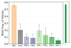
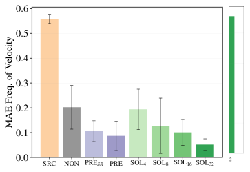
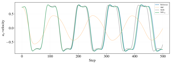
Due to the distinct vortex shedding characteristics of the flow, it is interesting to evaluate the flow field in terms of its frequency spectrum. As an example, Fig. 7 shows the $u_{x}$ velocity component over the course of 500 simulation steps at the center of domain, i.e., behind the obstacle, for one of our test data sets. We show the corresponding evaluation in Fig. 8. Interestingly, especially the PRE versions fare better in terms of frequency errors. Here the relatively expensive pre-computation step shows a performance gain. Nonetheless, the models trained via differentiable physics likewise learn to control the frequency behavior when training with a sufficient number of look-ahead steps as the SOL₃₂ model yields a substantially lower frequency error than the PRE model.

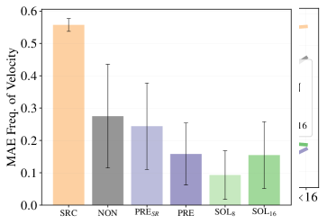
We additionally show results for a smaller model for a simpler sequential convolutional network with 57k trainable parameters in Fig. 9. The overall relative ordering of the interaction methods remains the same. The non-interacting method performs worse than pre-computation, which in turn is outperformed by the differentiable physics interaction. However, the overall performance is reduced, e.g., the NON model only reduces the error by ca. 30%. The SOL₁₆ version still outperforms the other versions. Overall, not surprisingly, the reduced weight count significantly reduces the representational capabilities of the neural networks and leads to a deteriorated performance. Nonetheless, training via interactions with differentiable physics is beneficial for inference performance.

To conclude, approximate solutions of the unsteady wake flow case can be corrected substantially by learned models, and especially training with differentiable physics in the loop yields significantly reduced errors in long simulated sequences. The SOL₃₂ version with a larger model reduces the MAE with respect to the reference solution to less than 9% (on average) of the error induced by the source simulation.

(a) Velocity error for different models

(b) Velocity improvement (relative to SRC) for different models

Figure 5: Different models applied to five test cases over 500 time steps for the unsteady wake flow scenario. The SOL₃₂ reduces the error introduced by SRC by a factor of 11.2 on average.

(a) Velocity error per Reynolds number

(b) Velocity improvement (relative to SRC) per Reynolds number

Figure 6: Separate evaluations for five different test cases of the unsteady wake flow scenario.

Figure 7: $u_{x}$-velocity at the center of domain for one test data set (Re = $\times 4$).

(a) Frequency error for different models

(b) Frequency error per Reynolds number

Figure 8: Frequency-domain evaluation for the unsteady wake flow scenario. Shown for the five test cases over 500 time steps.

(a) Velocity error for different smaller models

(b) Smaller models per Reynolds number

Figure 9: Different models with a smaller network size (57k trainable weights) applied to five test cases over 500 time steps for the unsteady wake flow scenario.

\begin{overpic}[width=416.27809pt]{figs/summary-karman-training-data.jpg} \put(-1.6,0.0){\scriptsize\rotatebox{90.0}{\makebox[10.66pt]{Reference}}} \put(-1.6,10.66){\scriptsize\rotatebox{90.0}{\makebox[10.66pt]{SRC}}} \put(100.5,0.0){\includegraphics[height=10.66pt]{figs/summary-legend-karman}} \end{overpic}

Figure 10: An example sequence of the unsteady wake flow from the training data set for time steps $t\in\{50,60,\cdots,200\}$.

\begin{overpic}[width=416.27809pt]{figs/summary-karman-test-data-b.jpg} \put(0.0,30.0){(a)} \put(-1.6,0.0){\scriptsize\rotatebox{90.0}{\makebox[10.66pt]{Reference}}} \put(-1.6,10.66){\scriptsize\rotatebox{90.0}{\makebox[10.66pt]{SOL${}_{32}$}}} \put(-1.6,21.33){\scriptsize\rotatebox{90.0}{\makebox[10.66pt]{SRC}}} \put(100.5,0.0){\includegraphics[height=10.66pt]{figs/summary-legend-karman}} \end{overpic}

\begin{overpic}[width=416.27809pt]{figs/summary-karman-test-data.jpg} \put(0.0,30.0){(b)} \put(-1.6,0.0){\scriptsize\rotatebox{90.0}{\makebox[10.66pt]{Reference}}} \put(-1.6,10.66){\scriptsize\rotatebox{90.0}{\makebox[10.66pt]{SOL${}_{32}$}}} \put(-1.6,21.33){\scriptsize\rotatebox{90.0}{\makebox[10.66pt]{SRC}}} \put(100.5,0.0){\includegraphics[height=10.66pt]{figs/summary-legend-karman}} \end{overpic}

Figure 11: Time steps of test cases for the unsteady wake flow for $t\in\{50,60,\cdots,200\}$: (a) Re = $\times 1$ and (b) Re = $\times 16$.

Table 2: Quantitative evaluation of different models for the unsteady wake flow scenario.

Model	MAE Velocity, Mean (std. dev.)
	SRC	NON	PRE${}_{\text{SR}}$	PRE	SOL4	SOL8	SOL16	SOL32
Regular	0.146	0.049	0.036	0.031	0.041	0.031	0.023	0.013
	(0.004)	(0.012)	(0.009)	(0.010)	(0.009)	(0.012)	(0.004)	(0.003)
Smaller	0.146	0.092	0.083	0.059	-	0.042	0.035	-
	(0.004)	(0.028)	(0.025)	(0.015)	-	(0.011)	(0.010)	-
	$L^{2}$ Error of $u_{x}$ Velocity in Frequency Domain
	SRC	NON	PRE${}_{\text{SR}}$	PRE	SOL4	SOL8	SOL16	SOL32
Regular	0.557	0.202	0.106	0.087	0.194	0.128	0.101	0.051
Smaller	0.557	0.275	0.244	0.158	-	0.093	0.155	-

B.2 Buoyancy-driven Fluid Flow

This scenario encompasses a volume of hot smoke rising in a closed container. The motion of the smoke volume is driven by buoyancy forces computed via a marker field that is passively advected in the flow, and which marks a region of fluid with lower density. Assuming a small relative change of density between the marker and the bulk, we compute the resulting forces with a Boussinesq model. Hence, this scenario is likewise based on the Navier-Stokes equations, but due to the additional coupled system, it leads to significantly more chaotic and complex behavior than the unsteady wake flow. In order to target solutions with complex motions, we do not explicitly solve for viscosity effects, but rely on the numerical viscosity inherent in the discretization. This yields the following PDE:

$$\frac{\partial u_{x}}{\partial{t}}+{\bm{u}}\cdot\nabla u_{x}=-\frac{1}{\rho}\nabla{p},\quad\frac{\partial u_{y}}{\partial{t}}+{\bm{u}}\cdot\nabla u_{y}=-\frac{1}{\rho}\nabla{p}+\eta d$$

$$\text{subject to}\quad\nabla\cdot{\bm{u}}=0,\quad\frac{\partial d}{\partial{t}}+{\bm{u}}\cdot\nabla d=0\ ,$$ (14)

where $\eta$ denotes the buoyancy factor for the Boussinesq model.

We also use this scenario to demonstrate that the reference data can be computed by a discretization or algorithm that differs from the one used to compute the source trajectories. More specifically, we use second-order pressure projection scheme for the reference trajectory solutions [78], which was shown to lead to an improved conservation of energy [22]. In addition, we use a less dissipative advection scheme for the source and reference solvers [58].

The domain has an extend of $1\times 2$ units, where the marker density is injected in the lower quadrant. The reference simulations use a staggered discretization with $d_{r,x}=128$ and $d_{r,y}=256$, while the source simulations use a domain with $d_{s,x}=32$ and $d_{r,y}=64$. We randomize the initial size of the marker volumes with circular shapes with a radius $r\sim\mathcal{U}(0.1,0.25)$, where $\mathcal{U}$ denotes a uniform distribution. The training data set consists of 48 different initial conditions simulated for 1000 steps each. Several examples are shown in Fig. 15. For the test scenes, we change the initial marker distribution $d$ to obtain five simulations containing two circles with $r\sim\mathcal{U}(0.05,0.1)$ and another five simulations with $r\sim\mathcal{U}(0.2,0.3)$. Thus, we obtain ten test scenes, half of which have a reduced marker quantity compared to the training data and five with an increased quantity. As the $d$ determines the forces induced by the Boussinesq model, this leads to simulations that are slower and faster, respectively, than those in the training set.

Training Procedure

The neural network architecture for $\mathcal{C}$ follows the one described above, but instead uses four ResBlocks with 16 features each and contains ca. 36k trainable weights. As both velocity ${\bm{u}}$ and marker $d$ determine the dynamics of the flow, the network receives both fields as input, but still only infers a correction for the velocity; i.e., $d$ is modified only via advection through ${\bm{u}}$, not directly by $\mathcal{C}$. All SOL and NON models are trained for 294k iterations with a batch size of 4 and a learning rate of $10^{-4}$. We evaluate the models on validation set with 5 simulations and 300 time steps drawn from the same initial marker distribution as the training data, and keep the model with the lowest validation loss.

To speed up the pre-computations, we only compute $\mathcal{C}_{\text{pre}}$ for cells $i,j$ in the domain with $d_{i,j}>10^{-4}$ (we validate this choice below). The PRE variants of $\mathcal{C}$ are then trained on the resulting, regularized data for 300k iterations with a batch size of 32 using horizontal flipping as data augmentation.

Results

We evaluate different models which are applied to 300 time steps of ten test conditions. Errors with respect to the reference solutions are computed and averaged across the resulting 3k phase field states. Numeric error values for the following tests can be found in Table 3.

We evaluate the different baseline versions (NON and PRE) in comparison to the source simulation (which underlies all other variants) and compare them to SOL versions with increasing look-ahead. The resulting errors and relative improvements are shown in Fig. 12 and given numerically in Table 3. It is apparent that the SOL versions yield very significant improvements over the other learned variants. Besides the velocity errors, we also provide an evaluation of the passively advected marker density $d$. This quantity is crucial for the dynamics of the flow, but cannot be influenced directly by the neural networks. Hence, it provides an additional view on how well the inferred corrections manage to reduce the numerical errors of the source simulation. The corresponding evaluation highlights that both velocity and density improvements increase consistently with SOL variants that were trained with larger look-aheads. We also evaluate the different models in terms of kinetic energy of the flows. As the kinetic energy is agnostic to the direction of the flow, the residual errors of the different variants do not show up as clearly as in the other evaluations. However, while the density and kinetic energy improvements are smaller than those for the velocity fields, the SOL₁₂₈ model nonetheless clearly outperforms the other variants.

Visualized evolutions of several test simulations are shown in Fig. 16. Here, the bi-modal nature of the test data with smaller (b) and larger (a,c) initial marker density configurations is shown. The different initial conditions lead to smaller and larger average velocities and, hence, highlight that the trained model generalizes very well.

Ablations

An evaluation of different neural network architectures for the buoyancy-driven flows with SOL₂ interaction illustrates how improvements stagnate beyond a certain network size and depth. For example, a model with more than 100k weights and almost three times the size of the regular model only yields an improvement of 3.6%. Another increase by a factor of four only gives 0.3% improvement. The corresponding graphs can be found in Fig. 13. Decreasing the network size, on the other hand, yields a performance that is 8.7% lower or even more for the smallest model. This motivates our choice to focus on the architecture with 36k trainable parameters, which was used for all other test with the buoyancy-driven flows.

As discussed in the main text, we also evaluated a method proposed by Sanchez et al. [55] to perturb inputs to network with noise in order to stabilize predictions. This approach shares our goal to reduce the shift of distributions for the input data such that the trained networks can produce more reliable estimates as they encounter new inputs at inference time. However, in contrast to the Lagrangian graph-based physics predictions, the added noise did not lead to large gains in our context. We test a variety of trained SOL₂ networks for which noise was injected into the input features, i.e., cell-wise samples of velocity and marker density, from a component-wise normal distribution $\mathcal{N}(0,\sigma)$ with standard deviation $\sigma$.

Details of the results are visualized in Fig. 14. As can be seen in the results, there is only a slight positive effect across a wide range of different noise strengths. The networks with $\sigma\sim 10^{-4}$ show the best results. However, the improvements of up to 34.6% via noise perturbations are surpassed by the SOL_n models, where the best one yields an improvement of 59.8%. We think that the gains of our interacting model compared to injecting noise come from the systematic improvements of the SOL training, which potentially provides more reliable inputs at training time than stochastic perturbations. The fully convolutional nature of the networks additionally provides regularization at training time.

We have also evaluated how sub-optimal choices for solver interactions affect the inference performance. We train several NON models that are allowed to evolve for $n$ time steps without interaction, while computing a regular $L^{2}$ loss via Eq. 3. These versions are denoted with NON_dn for $n$ steps of diverging evolution. In addition, we evaluate a model PRE${}_{\text{\text{SR}}}$ using a pre-computed interaction without temporal regularization (i.e., only spatial) and one version (PRE${}_{\text{\text{F}}}$) that uses the full spatiotemporal regularization without a density threshold; i.e., it requires several times more pre-computation by solving the Lagrange-multiplier minimization for the full spatial domains. Especially, the NON_dn variants perform badly and exhibit large errors, with NON_d8 significantly distorting the flow behavior, instead of improving it. The corresponding evaluations are visualized in Fig. 17. It is likewise apparent that the additional PRE variants deteriorate the ability of the ANNs to correct the numerical errors of the source simulations.

To summarize, despite the complexity of the buoyancy-driven flows and the difficult reference trajectories produced by a higher-order PDE solver, the numerical errors of the source simulation can be reduced very successfully by training with the solver in the training loop.

(a) Velocity error

(b) Marker advection error

(c) Kinetic energy error

(d) Velocity improvement

(e) Impr. of marker advection

(f) Impr. of kin. energy

Figure 12: Velocity, marker advection, and kinetic energy errors for different models, especially for different SOL versions with increasing look-ahead. In the second row, we show improvements relative to the source version SRC.

(a) Trainable weights

(b) Velocity error

(c) Marker error

(d) Velocity improvement

Figure 13: SOL₂ training with different architectures that strongly vary the number of trainable parameters (a). While the smaller two models lead to a clear drop in accuracy, the larger two architectures yield small gains despite the increased weight count.

(a) Velocity improvement

(b) Improvement of marker advection

Figure 14: Varying levels of noise injected into the input features for SOL₂ at training time. While values around $10^{-4}$ lead to slight positive effects, the improvements are negligible compared to those achievable by the SOL variants.

\begin{overpic}[width=416.27809pt]{figs/summary-smoke-training-data} \put(-1.6,0.0){\scriptsize\rotatebox{90.0}{\makebox[6.71pt]{Ref.}}} \put(-1.6,6.71){\scriptsize\rotatebox{90.0}{\makebox[6.71pt]{SRC}}} \put(100.5,0.0){\includegraphics[height=6.71pt]{figs/summary-legend-buoy}} \end{overpic}

Figure 15: An example sequence of the buoyancy scenario from the training data set for time steps $t\in\{0,25,\cdots,375\}$.

\begin{overpic}[width=416.27809pt]{figs/summary-smoke-test-data} \put(0.0,18.0){{\color[rgb]{1,1,1}(a)}} \put(-1.6,0.0){\scriptsize\rotatebox{90.0}{\makebox[6.71pt]{Ref.}}} \put(-1.6,6.71){\scriptsize\rotatebox{90.0}{\makebox[6.71pt]{SOL${}_{128}$}}} \put(-1.6,13.43){\scriptsize\rotatebox{90.0}{\makebox[6.71pt]{SRC}}} \put(100.5,0.0){\includegraphics[height=6.71pt]{figs/summary-legend-buoy}} \end{overpic}

\begin{overpic}[width=416.27809pt]{figs/summary-smoke-test-data-b} \put(0.0,18.0){{\color[rgb]{1,1,1}(b)}} \put(-1.6,0.0){\scriptsize\rotatebox{90.0}{\makebox[6.71pt]{Ref.}}} \put(-1.6,6.71){\scriptsize\rotatebox{90.0}{\makebox[6.71pt]{SOL${}_{128}$}}} \put(-1.6,13.43){\scriptsize\rotatebox{90.0}{\makebox[6.71pt]{SRC}}} \put(100.5,0.0){\includegraphics[height=6.71pt]{figs/summary-legend-buoy}} \end{overpic}

\begin{overpic}[width=416.27809pt]{figs/summary-smoke-test-data-c} \put(0.0,18.0){{\color[rgb]{1,1,1}(c)}} \put(-1.6,0.0){\scriptsize\rotatebox{90.0}{\makebox[6.71pt]{Ref.}}} \put(-1.6,6.71){\scriptsize\rotatebox{90.0}{\makebox[6.71pt]{SOL${}_{128}$}}} \put(-1.6,13.43){\scriptsize\rotatebox{90.0}{\makebox[6.71pt]{SRC}}} \put(100.5,0.0){\includegraphics[height=6.71pt]{figs/summary-legend-buoy}} \end{overpic}

Figure 16: Several time steps $t\in\{50,60,\cdots,200\}$ of three buoyancy-driven fluid flow test cases (a)-(c).

(a) Velocity error

(b) Density error

(c) Velocity improvement

Figure 17: A comparison of models trained with a variety of sub-optimal interaction schemes for the buoyancy scenario. NON_dn allows non-interacting models to evolve and diverge over $n$ steps, while PRE${}_{\text{SR}}$ employs only spatial regularization in the pre-computation. PRE${}_{\text{F}}$ resembles PRE, but was trained without a density threshold. Especially, the changes relative to SRC in (c) highlight that the NON_dn variants have a negative effect.

Table 3: Quantitative evaluation of models for the buoyancy-driven flow scenario. M_XS,S,L,XL denote different model sizes, while $\sigma_{1,2,3}$ denote models trained with noise of $\sigma=10^{-3,-4,-5}$.

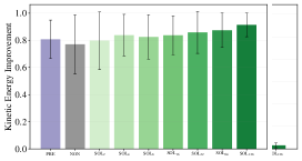
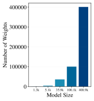
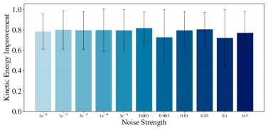
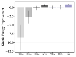
Quantity	MAE Velocity, Mean (std. dev.)
	SRC	NON	PRE	SOL2	SOL16	SOL32	SOL64	SOL128
Velocity	1.590	1.079	1.373	1.027	0.859	0.775	0.695	0.620
	(1.032)	(0.658)	(0.985)	(0.656)	(0.539)	(0.482)	(0.420)	(0.389)
Marker $d$	0.677	0.499	0.579	0.484	0.430	0.419	0.401	0.391
	(0.473)	(0.336)	(0.409)	(0.325)	(0.281)	(0.277)	(0.262)	(0.253)
	MXS	MS	ML	MXL	$\sigma_{1}$	$\sigma_{2}$	$\sigma_{3}$	NONd4
Velocity	1.228	1.193	0.982	0.969	1.070	1.056	1.078	3.196
	(0.746)	(0.826)	(0.646)	(0.626)	(0.683)	(0.700)	(0.706)	(1.404)
Marker $d$	0.521	0.494	0.461	0.466	0.503	0.496	0.503	0.656
	(0.352)	(0.349)	(0.313)	(0.318)	(0.341)	(0.339)	(0.345)	(0.426)

B.3 Forced Advection-Diffusion

In the forced advection-diffusion scenario, we target a PDE environment with a constant, randomized forcing term. This forcing continuously injects energy into the dissipative system and takes the form of a spectrum of parametrized bands of sine waves. In this scenario, we target Burgers’ equation. It represents a well-studied advection-diffusion PDE:

$$\frac{\partial u_{x}}{\partial{t}}+{\bm{u}}\cdot\nabla u_{x}=\nu\nabla\cdot\nabla u_{x}+g_{x}(t),\quad\frac{\partial u_{y}}{\partial{t}}+{\bm{u}}\cdot\nabla u_{y}=\nu\nabla\cdot\nabla u_{y}+g_{y}(t),$$ (15)

where $\nu$ and $\mathbf{g}$ denote diffusion constant and external forces, respectively. Our setup resembles a 2D variant of the tests employed by the work on learning data-driven discretizations [4]; correspondingly, we extend the forcing terms described there to 2D. We generate the forces from 20 overlapping sine functions each with a random direction, amplitude, and phase shift:

$$g_{x}(t)=\sum_{i=1}^{20}\cos(\alpha_{i})a_{i}\sin(\omega_{i}t-kx+\phi_{i}),\quad g_{y}(t)=\sum_{i=1}^{20}\sin(\alpha_{i})a_{i}\sin(\omega_{i}t-kx+\phi_{i}).$$ (16)

This PDE scenario does not involve any equality constraints, i.e., ${\bm{M}}=0$.

Similar to the previous scenarios, we discretize the system on a staggered grid and compute the advection operator with a semi-Lagrangian scheme [61]. The domain has a square, normalized size of $1\times 1$ with reference trajectories computed via a resolution of $d_{r,x}\!=\!d_{r,y}\!=\!128$. The source domain correspondingly uses $d_{s,x}\!=\!d_{s,y}\!=\!32$.

Training Procedure and Results

As training data, ten simulations of 200 steps each are used. An example sequence of the data is shown in Fig. 18. The SOL and NON models are trained for 38.4k steps with a batch size of five with a learning rate of $10^{-4}$, while the PRE model is trained for 25k steps with a batch size of 32 using an initial learning rate of $10^{-3}$ that was lowered to $5\times 10^{-7}$ over the course of the training. The PRE model additionally uses 5% of the training data set for validation. The test data set contains five cases with different initial conditions and force fields over the course of 200 time steps. All models use a neural network architecture with five ResBlocks with 32 features each.

As summarized in the main text, the learned correction functions can significantly decrease the numerical errors of the source simulation. Across the different test cases (partly shown in Fig. 19), the best models achieve a reduction by over 67%. The corresponding MAE measurements are given in Table 4, and Fig. 20 provides an overview of the performance per test case. While the PRE model shows a lower performance, most likely due to an overly strong temporal regularization, the NON model is close to the best SOL model in this case with an MAE of 0.159 compared to 0.148 for SOL₂. Interestingly, this behavior matches the results of Bar-Sinai et al. [4]. They experimented with up to eight recurrent steps of a 1D Burgers’ simulation, but did not report significant advantages from training with the 1D solver in the loop.

In contrast, we found that more interactions show their advantage in a deterministic scenario, where we exclude the external forces from the Burgers’ equation above, i.e., Eq. 15. As this versions exhibits less chaotic behavior, the SRC version generally shows smaller errors compared to the SRC version in the forced scenario. The SOL versions now yield further improvements when trained with more look-ahead: SOL₄ yields an improvement of 10% over SRC, SOL₁₆ yields 12%, while the SOL₃₂ version reduces the error by 17%. Table 4 shows the corresponding MAE measurements.

Our results highlights that deep learning via physical simulations works particularly well when the ANNs can actually learn to predict the behavior of the dynamics and, thus, compensate for the numerical errors that will occur. If, on the other hand, external and unpredictable influences such as the randomized forcing terms dominate the behavior, the model has a reduced chance to predict the right correction function.

Table 4: Quantitative evaluation of different models for the forced advection-diffusion scenario. MAE values without forcing are given with a $\times 100$ factor.

MAE Velocity, Mean (std. dev.)
With forcing	SRC	PRE	NON	SOL2	SOL4	SOL8
	0.248	0.218	0.159	0.148	0.152	0.158
	(0.019)	(0.017)	(0.015)	(0.016)	(0.015)	(0.017)
Without forcing	SRC	NON	SOL4	SOL8	SOL16	SOL32
$(\times 100)$	0.306	0.272	0.276	0.277	0.268	0.253
	(0.020)	(0.028)	(0.037)	(0.040)	(0.030)	(0.020)

\begin{overpic}[width=416.27809pt]{figs/summary-burgers-training-data.jpg} \put(-1.6,0.0){\scriptsize\rotatebox{90.0}{\makebox[7.14pt]{Ref.}}} \put(-1.6,7.14){\scriptsize\rotatebox{90.0}{\makebox[7.14pt]{SRC}}} \put(100.5,0.0){\includegraphics[height=7.14pt]{figs/summary-legend-burgers}} \end{overpic}

Figure 18: An example sequence from the training data set of the forced advection-diffusion test case.

\begin{overpic}[width=416.27809pt]{figs/summary-burgers-test-data.jpg} \put(100.0,19.0){(a)} \put(-1.6,0.0){\scriptsize\rotatebox{90.0}{\makebox[7.14pt]{Ref.}}} \put(-1.6,7.14){\scriptsize\rotatebox{90.0}{\makebox[7.14pt]{SOL${}_{2}$}}} \put(-1.6,14.28){\scriptsize\rotatebox{90.0}{\makebox[7.14pt]{SRC}}} \put(100.5,0.0){\includegraphics[height=7.14pt]{figs/summary-legend-burgers}} \end{overpic}

\begin{overpic}[width=416.27809pt]{figs/summary-burgers-test-data-b.jpg} \put(100.0,19.0){(b)} \put(-1.6,0.0){\scriptsize\rotatebox{90.0}{\makebox[7.14pt]{Ref.}}} \put(-1.6,7.14){\scriptsize\rotatebox{90.0}{\makebox[7.14pt]{SOL${}_{2}$}}} \put(-1.6,14.28){\scriptsize\rotatebox{90.0}{\makebox[7.14pt]{SRC}}} \put(100.5,0.0){\includegraphics[height=7.14pt]{figs/summary-legend-burgers}} \end{overpic}

\begin{overpic}[width=416.27809pt]{figs/summary-burgers-test-data-c.jpg} \put(100.0,19.0){(c)} \put(-1.6,0.0){\scriptsize\rotatebox{90.0}{\makebox[7.14pt]{Ref.}}} \put(-1.6,7.14){\scriptsize\rotatebox{90.0}{\makebox[7.14pt]{SOL${}_{2}$}}} \put(-1.6,14.28){\scriptsize\rotatebox{90.0}{\makebox[7.14pt]{SRC}}} \put(100.5,0.0){\includegraphics[height=7.14pt]{figs/summary-legend-burgers}} \end{overpic}

Figure 19: Time steps of three test cases (a)-(c) from the forced advection-diffusion scenario.

(a) Velocity error per test case

(b) Velocity improvement (relative to SRC) per test case

Figure 20: Separate evaluations for five different test cases of the forced advection-diffusion scenario.

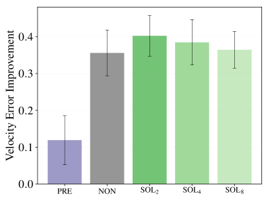
B.4 Inference of Initial Guesses for Conjugate Gradient Solvers

In this section, we investigate the interaction of learning models with conjugate gradient (CG) solvers [26]. We target Poisson problems, which often arise many PDEs, e.g., in electrostatics or in fluid flow problems where the pressure $p$ is computed via $\nabla\cdot\nabla p=\nabla\cdot{\bm{u}}$. Specifically, we explore the iteration behavior of the CG solver given an initial state predicted by a trained model. To this end, we compare three main methods: A solver-in-the-loop (SOL_n) approach, a non-interacting supervised approach (NON), and a differentiable physics-based (SOL${}_{\text{DIV}}$), which is trained to directly minimize the PDE residual. In general, the CG solver iterations converge toward a reference pressure field $p$ such that ${\bm{A}}p=\nabla\cdot{\bm{u}}$ with ${\bm{A}}=\nabla\cdot\nabla$. For an intermediate solution $\hat{p}$, the residual $r=\nabla\cdot{\bm{u}}-{\bm{A}}\hat{p}$ measures how far away the approximated pressure $\hat{p}$ is from the true solution. Thus, as the solver converges, $r$ decreases and the difference $\hat{p}-p$ converges to zero. In the following, we employ the neural network $\mathcal{C}$ to infer a pressure field given a velocity sample ${\bm{u}}$, i.e., $\hat{p}=\mathcal{C}({\bm{u}})$. We focus on 2D cases, i.e., ${\bm{u}}{}\in\mathbb{R}^{2\times d_{x}\times d_{y}}$ and $p,r\in\mathbb{R}^{d_{x}\times d_{y}}$.

Loss Functions

The NON version employs a regular supervised loss, i.e., the difference of the predicted pressure $\hat{p}$ from the pre-computed reference pressure $p$ for $j$ different samples:

$$\mathcal{L}_{\text{NON}}=\|\mathcal{C}({\bm{u}})-p\|^{2}.$$ (17)

We additionally compare to a variant that is often referred to as unsupervised in previous work, and which is in line with other physics-based or physics-informed loss constructions [49, 60]. Specifically, the SOL${}_{\text{DIV}}$ version replicates the setup described in [67] and uses the PDE $\nabla^{2}p-\nabla\cdot{\bm{u}}=0$ as loss for the training of a neural network. Given an input velocity ${\bm{u}}^{*}$, the goal is to infer a pressure function $\hat{p}(\nabla\cdot{\bm{u}}^{*})$ such that the PDE residual is minimized:

$$\mathcal{L}_{\text{SOL}_{\text{DIV}}}=\|\nabla\cdot{\bm{u}}^{*}-\nabla\cdot\nabla\mathcal{C}({\bm{u}})\|^{2}.$$ (18)

This version represents a different form of differentiable PDE solvers, namely including them in the loss formulation, and hence we denote it with SOL${}_{\text{DIV}}$. However, due to a lack of iterating calculations for this variant, a more appropriate name would be “solver-in-the-loss” rather than “solver-in-the-loop”.

As a third variant, we employ a solver-in-the-loop interaction that employs a differentiable CG solver and uses a learning objective to minimize the PDE residual after $n$ iterations of the CG solver. In this scenario, $\mathcal{P}_{s}$ represents a linear operator, i.e., one step of the CG method to approximate $\nabla^{-2}\,(\nabla\cdot{\bm{u}})$, and the loss function is given by:

$$\mathcal{L}_{\text{SOL}_{n}}=\|\mathcal{P}_{s}^{n}(\mathcal{C}({\bm{u}}))-\mathcal{C}({\bm{u}})\|^{2}.$$ (19)

Thus, the SOL_n and SOL${}_{\text{DIV}}$ both minimize the same residual divergence $r$; while the SOL${}_{\text{DIV}}$ loss aims to do so directly, the SOL_n version instead sees how the iterative solver performs. At training time, the SOL_n variant receives gradients through $n$ iterations of the iterative solver via back-propagation.

Training Procedure

The trained models in this section all use the same convolutional U-net architecture [54] with 22 layers of strided convolutions and 5$\times$5 kernels, containing around 127k trainable parameters (see App. D for details). The training data set was generated using the conjugate gradient solver from the $\Phi_{\textrm{Flow}}$ framework [27]. It is comprised of 3k fluid simulations on a domain with $d_{x}=d_{y}=64$ and closed boundaries. Each simulation consists of a randomly generated density and velocity field, which are integrated over time for 16 steps. Each model was trained for 300k steps with a learning rate of $2\times 10^{-4}$ and training batch size of 16. The reference solutions were pre-computed with a CG solver using an accuracy threshold of $10^{-6}$ for the residual norm.

Results

We now compare the different loss functions by their performance in conjunction with the CG solver. We compute averages for 100 test cases each time, i.e., samples that were not seen at training time. As baseline, we denote a CG solving process that starts from a zero guess as SRC.

We first compare how many CG iterations are required to reach a certain target accuracy given the inferred solutions by the three different types of models. The results are shown in Table 5 and visualized in Fig. 21. Initially, SOL${}_{\text{DIV}}$ reaches an accuracy of almost $10^{-2}$, closely followed by SOL₅. While the supervised NON version produces pressure predictions that seem quite close to the reference, its initial accuracy is only slightly better than the zero guess employed by SRC. This is due to the error being measured locally per grid point, while the correctness of larger structures becomes more important after in interactions with the CG solvers. Over the first five to ten CG iterations, the accuracy of SOL₅ improves very quickly, overtaking the other methods. To reach an accuracy of $10^{-2}$, the CG solver requires an average of around two steps in conjunction with SOL₅, nine steps with NON, 28 steps with SOL${}_{\text{DIV}}$ and 78 steps starting from zero. When running the CG solver for more iterations, the accuracy increases similarly for all methods, with SOL₅ retaining its advantage.

Comparing SOL₅ to SOL${}_{\text{DIV}}$ shows the importance of training with the solver in the loop: the SOL${}_{\text{DIV}}$ model does not receive any feedback regarding the behavior of the solver. It predicts solutions that satisfy the loss – measured per grid point – but do not match the large-scale structures of the true solution. Consequently, this task is left to the CG solver, which requires many iterations to work out the correct global solution. The SOL₅ model, however, sees the corrections performed by the CG solver at training time and can learn to adjust its guess accordingly.

When investigating the inferred pressure fields themselves (Fig. 22), we see that the guesses of the SOL₅ model come closest to the reference, followed by those of the NON variant. The SOL${}_{\text{DIV}}$ differs more strongly, and the residual divergence, shown in Fig. 23, highlights that it has a noticeable error pattern near the outer border of the domain. This provides an explanation for the poor behavior of the SOL${}_{\text{DIV}}$ model for the initial CG solver iterations: while it minimizes the PDE-based loss in an absolute sense, it does not receive information about how different parts of the solution influence the future iterations of the solver. This ambiguity is alleviated to some extent by the pre-computed reference solutions for NON, but especially the SOL₅ version receives this feedback in terms of gradient from the differentiable solver and, in this way, can best adapt to the requirements for future iterations.

We also experimented with varying the number of look-ahead steps for SOL_n models in the loss function of Eq. 19. This ablation study (Fig. 24) shows how too few iterations clearly deteriorate the performance, while more than 5 iterations lead to a slight increase in the required iterations. We assume that this behavior is potentially caused by evaluating the loss only for the final output of the $n$ iterations.

Discussion

Our results highlight the advantages of training with the solver in the loop for fully implicit PDE solvers. Likewise, it shows that a physics-informed loss formulation alone yields only a partial view of the problem. While a loss-based residual cannot adapt to iterative algorithms, the solver-in-the-loop models directly receive gradient-based feedback at training time.

The combination of an inferred initial guess with a traditional solver represents a particularly interesting hybrid algorithm, as it gives convergence guarantees that a learned approach alone would not be able to provide. Even if a trained model generates a sub-optimal solution, the solver can improve the solution until it matches the desired accuracy threshold. On the other hand, pre-training a model for a known problem domain can significantly reduce the required number of iterations and, consequently, reduce the workload in scenarios where PDEs from the same problem domain need to be solved repeatedly and in large numbers. Here, the current hardware developments provide an additional promise: the advances in terms of highly specialized hardware for evaluating neural networks can provide a substantial future speed-up even for a fixed, pre-trained model.

\begin{overpic}[width=195.12767pt]{figs/cg-iterations} \put(-5.0,55.0){(a)} \end{overpic}

\begin{overpic}[width=195.12767pt]{figs/cg-residuum-iterations} \put(-5.0,55.0){(b)} \end{overpic}

Figure 21: (a) Iterations needed to reach target accuracy and (b) comparison of maximum residual error over iterations.

\begin{overpic}[width=242.82613pt]{figs/cg-pressure-images} \put(-1.0,55.0){(a)} \end{overpic}

\begin{overpic}[width=186.45341pt]{figs/cg-pressure-differences} \put(-5.0,73.0){(b)} \end{overpic}

Figure 22: (a) Sample outputs of the models and (b) difference of output from reference.

Figure 23: Residual error after one CG solver iteration.

Figure 24: Comparison of SOL models with different look-ahead steps.

Table 5: Evaluation of the CG solver performance for different models.

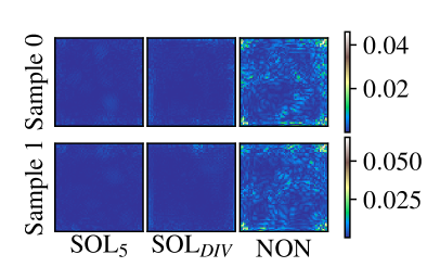
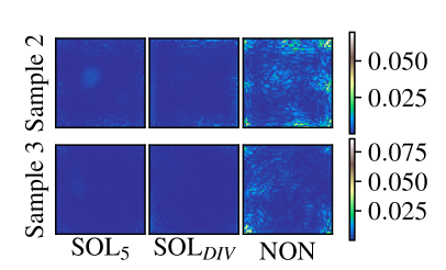
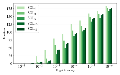
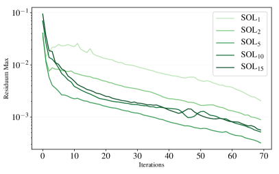
Model	Iterations for Accuracy, Mean (std. dev.)
	$10^{-1}$	$10^{-2}$	$10^{-3}$	$10^{-4}$	$10^{-5}$	$10^{-6}$
NON	1.67	9.33	52.16	109.12	155.37	186.12
	(1.010)	(5.428)	(17.540)	(15.875)	(10.155)	(5.719)
SOL${}_{\text{DIV}}$	0.0	27.79	79.06	117.97	155.76	181.07
	(0.0)	(15.255)	(10.042)	(13.234)	(9.403)	(6.052)
SOL5	0.03	1.97	29.59	88.37	133.59	167.37
	(0.171)	(1.118)	(14.832)	(13.465)	(11.605)	(8.549)

B.5 Three-dimensional Unsteady Wake Flow

As a final scenario, we target a three-dimensional fluid flow problem. The third spatial dimension leads to a large increase in terms of degrees of freedom, especially in the finer reference manifold. Additionally, the three axes of rotation lead to significantly more complicated flow structures.

Overall, we target a setup that represents an extension of the 2D unsteady wake flow case of App. B.1. Instead of a circular obstacle, the flow now faces a cylindrical obstacle in a 3D domain with extent of $1\times 1\times 2$. The cylinder with diameter $0.1$ is located at position $(1/2,1/2,0)^{T}$ and has an extent of 1 unit along the z-axis. We use the incompressible Navier-Stokes equations in three dimensions as underlying PDE:

$$\frac{\partial u_{x}}{\partial{t}}+{\bm{u}}\cdot\nabla u_{x}=-\frac{1}{\rho}\nabla{p}+\nu\nabla\cdot\nabla u_{x}$$

$$\frac{\partial u_{y}}{\partial{t}}+{\bm{u}}\cdot\nabla u_{y}=-\frac{1}{\rho}\nabla{p}+\nu\nabla\cdot\nabla u_{y}$$

$$\frac{\partial u_{z}}{\partial{t}}+{\bm{u}}\cdot\nabla u_{z}=-\frac{1}{\rho}\nabla{p}+\nu\nabla\cdot\nabla u_{z}$$

$$\text{subject to}\quad\nabla\cdot{\bm{u}}=0.$$ (20)

For reference simulations, the domain is discretized with $d_{r,x}\!=\!d_{r,y}\!=\!128$ and $d_{r,z}\!=256$ cells using a staggered layout for the velocity components. The source domain has a resolution of $d_{s,x}\!=\!d_{s,y}\!=\!32$ and $d_{r,z}\!=64$ cells. Data sets from both domains contain phase space trajectories of 500 time steps. For the training data, the viscosity coefficient $\nu$ is chosen to yield Reynolds numbers Re${}_{\text{train}}\in\{58.6,78.1,117.2,156.3,234.4,312.5,468.8,625.0\}$. While the range of Reynolds numbers covers a slightly reduced range compared to the 2D case, there is still a factor of more than ten between largest and smallest ones, and the 3D nature of the flow introduces a significant amount of complexity. The example visualizations of a training data set in Fig. 25 highlight the complexity of the flows.

For the test set, we use different Reynolds numbers, namely Re${}_{\text{test}}\in\{$68.4, 97.7, 195.3, 136.7, 273.4, 390.6, 546.9$\}$. The following test evaluations were computed for the seven Reynolds numbers in Re${}_{\text{test}}$ over 300 time steps. Numeric values are given in Table 6.

Training Procedure

For the 3D case, we use a ResNet that largely follows the architecture of the 2D cases, but employs 3D convolutions instead. The ResNet contains six blocks with kernel sizes of 5$\times$5$\times$5 and 3$\times$3$\times$3 for the two convolutional layers per block. The number of filters is increases to 48 in the center of the network, yielding 1002k trainable parameters (also see App. D). As for the 2D case, the inputs for the 3D models contain a constant field indicating the targeted Reynolds number. All models were trained for 300k iterations using a learning rate of $10^{-4}$ and a batch-size of four. We then use three validation simulations with Re${}_{\text{val}}\in\{$61.0 , 305.2 , 470.0$\}$ to select the best performing model.

Due to the increased computational workload to train the 3D models, we focus on a NON variant and a SOL₁₆ version, which uses the same differentiable Navier-Stokes solver for producing gradient information over the course of up to 16 unrolled simulation and inference steps for each iteration at training time. This version was trained with SOL₈ for 200k iterations and then for an additional 100k iterations as SOL₁₆.

Results

The 3D flow represents a significant increase in terms of complexity for the deep learning models. Among others, we were not able to train a stable NON version despite numerous tests. While the models performed well for ca. 100 to 150 time steps, small scale oscillations induced by the corrections accumulate and start to strongly distort the flow. This is a good example of the undesirable shift of distributions for the inputs: once the phase space trajectories produced by the hybrid method leave the distribution of the regular source states seen at training time, the model fails to infer reasonable corrections.

In contrast, the SOL₁₆ version retains its stability over the course of long simulations with several hundred steps. This is reflected in the MAE measurements of the velocity fields over the test cases: the regular source simulation induces an error of 0.167, which the NON version reduces to 0.143. The SOL₁₆ reduces the error to 0.130 instead, which however only gives a partial view of the overall behavior of the different versions. The graphs over time shown in Fig. 26(a) illustrate the diverging behavior of the NON version. While it does very well initially, even slightly surpassing SOL₁₆ around frame 100, the errors quickly grow afterwards, eventually leading to a performance that is worse than the source simulation.

The frequency graphs of the kinetic energy in Fig. 26(b), measured for an array of $5^{3}$ sample points at the center of the domain, instead show that the SOL₁₆ simulations closely match the frequency distribution of the reference simulations. It succeeds in restoring the change of frequencies across the different temporal scales of the flow significantly better than the SRC and NON models. The source simulation instead underestimates larger frequencies and over-estimates smaller ones.

Fig. 27 visualizes the vorticity magnitude of several test cases with Reynolds numbers not seen during training. The SOL₁₆ model manages to correct the vortex shedding behavior of the source simulation and closely matches the reference. As we visualize in the supplemental video, the NON version starts to oscillate, injecting undesirable distortions into the velocity field.

\begin{overpic}[width=433.62pt]{figs/karman3d-train01} \put(100.0,17.0){(a)} \put(-1.6,0.0){\scriptsize\rotatebox{90.0}{\makebox[11.65pt]{Reference}}} \put(-1.6,11.65){\scriptsize\rotatebox{90.0}{\makebox[11.65pt]{SRC}}} \put(100.5,0.0){\includegraphics[height=11.65pt]{figs/summary-legend-karman3d}} \end{overpic}

\begin{overpic}[width=433.62pt]{figs/karman3d-train04} \put(100.0,17.0){(b)} \put(-1.6,0.0){\scriptsize\rotatebox{90.0}{\makebox[11.65pt]{Reference}}} \put(-1.6,11.65){\scriptsize\rotatebox{90.0}{\makebox[11.65pt]{SRC}}} \put(100.5,0.0){\includegraphics[height=11.65pt]{figs/summary-legend-karman3d}} \end{overpic}

Figure 25: Two example sequences with (a) Re=117.2 and (b) Re=273.4 of the three-dimensional wake flow from the training data set. Each row shows 200 time steps for SRC (top) and reference versions (bottom) in terms of vorticity magnitude.

(a) Velocity error over time

(b) Frequency error

Figure 26: Evolutions of velocity MAE and frequency errors over the course of 300 time steps averaged for the seven test cases of the three-dimensional wake flow. (a) The NON versions perform well initially, but strongly diverges for later frames. (b) The SOL₁₆ shows a clearly improvement in terms of the frequency distribution of the kinetic energies. The overall curve of SOL₁₆ closely follows the reference with an initial offset over the reference, which inherits from the source simulation.

\begin{overpic}[width=433.62pt]{figs/karman3d-test00} \put(100.0,22.0){(a)} \put(-1.6,0.0){\scriptsize\rotatebox{90.0}{\makebox[11.65pt]{Ref.}}} \put(-1.6,8.0){\scriptsize\rotatebox{90.0}{\makebox[11.65pt]{SOL${}_{16}$}}} \put(-1.6,16.0){\scriptsize\rotatebox{90.0}{\makebox[11.65pt]{SRC}}} \put(100.5,0.0){\includegraphics[height=11.65pt]{figs/summary-legend-karman3d}} \end{overpic}

\begin{overpic}[width=433.62pt]{figs/karman3d-test03} \put(100.0,22.0){(b)} \put(-1.6,0.0){\scriptsize\rotatebox{90.0}{\makebox[11.65pt]{Ref.}}} \put(-1.6,8.0){\scriptsize\rotatebox{90.0}{\makebox[11.65pt]{SOL${}_{16}$}}} \put(-1.6,16.0){\scriptsize\rotatebox{90.0}{\makebox[11.65pt]{SRC}}} \put(100.5,0.0){\includegraphics[height=11.65pt]{figs/summary-legend-karman3d}} \end{overpic}

\begin{overpic}[width=433.62pt]{figs/karman3d-test06} \put(100.0,22.0){(c)} \put(-1.6,0.0){\scriptsize\rotatebox{90.0}{\makebox[11.65pt]{Ref.}}} \put(-1.6,8.0){\scriptsize\rotatebox{90.0}{\makebox[11.65pt]{SOL${}_{16}$}}} \put(-1.6,16.0){\scriptsize\rotatebox{90.0}{\makebox[11.65pt]{SRC}}} \put(100.5,0.0){\includegraphics[height=11.65pt]{figs/summary-legend-karman3d}} \end{overpic}

Figure 27: Three test cases with (a) Re=68.4, (b) Re=136.7, and (c) Re=546.9. Each row shows time steps over the course of 200 time steps for SRC, SOL₁₆, and the reference (top to bottom). The SOL₁₆ model interacting with the source solver successfully preserves the complex rotating motions behind the cylindrical obstacle (middle), which the regular source solver cannot resolve (top).

Table 6: Quantitative evaluation of different models for the three-dimensional wake flow scenario.

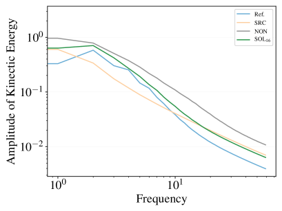
MAE Velocity, Mean (std. dev.)			Freq. MAE Kinetic Energy, Mean (std. dev.)
SRC	NON	SOL16	SRC	NON	SOL16
0.167 (0.035)	0.143 (0.070)	0.130 (0.024)	0.0614 (0.133)	0.074 (0.209)	0.058 (0.088)

Appendix C Performance

We measure the computational performance of our models in comparison to a reference simulation on a workstation with an Intel Xeon E5-1650 CPU with 12 virtual cores at 3.60GHz and an NVIDIA GeForce GTX 1080 Ti GPU. As reference solver, we employ a CPU-based simulator using OpenMP parallelization. We compare this with our (relatively un-optimized) differentiable physics framework, which evaluates the PDE and the trained model within TensorFlow on the GPU.

For the buoyancy-driven flow simulation, the CPU-based reference simulation requires 5.79 seconds on average for 100 time steps. Instead, evaluating the SOL₁₂₈ neural network model itself requires an accumulated 0.43 seconds. For comparison, computing 100 time steps of the source solver takes 0.476 seconds. In comparison to the inference for forward simulations with a pre-trained model, each iteration during training is significantly more expensive: for the SOL₈, SOL₁₆, and SOL₃₂ models of the 2D wake flow case, a training iteration took 0.6, 1.3, and 2.5 seconds on average, respectively. As this is a one-time, pre-processing cost, the gains in performance of the resulting hybrid solver can quickly offset the computational expense for training a model.

The computational workload for PDE solvers typically rises super-linearly with the number of degrees of freedom. Hence, the gap is even more pronounced when considering the 3D wake flow case. Here, the reference simulation requires 913.2 seconds for 100 time steps, while the SOL₁₆ version requires 13.3 seconds on average. Thus, the source simulation with learned corrections is more than 68 times faster than the reference simulation.

Despite the substantial reduction in terms of runtime, we believe these performance results are preliminary, and far from the speed-up that could be achieved in optimal settings with a learning-augmented PDE solver. An inherent advantage of combining an approximate PDE solver with a deep-learning-based corrector ANN stems from the fact that a relatively simple solver suffices as a basis. Hence, while existing reference solvers in scientific computing fields might come with vast existing code-bases, the source solver could encompass only a small subset of the full solver and introduce the residual dynamics via a learned component. This would also reduce the work to provide gradients for the source solver, which many existing simulation frameworks do not readily offer. Due to its reduced scope, the source solver would also be significantly easier to optimize. Additionally, the learned corrector component would trivially benefit from all future hardware advances for efficient evaluations of neural networks. Hence, we believe that, in practice, a much more substantial speed-up will be achievable than the ones we have measured for the two- and three-dimensional simulation scenarios of this work.

Appendix D Neural Network Architectures

Below, we give additional details of the network architectures used for the five different scenarios. We intentionally slightly vary the architecture to demonstrate that our solver-in-the-loop approach does not rely on a single, specific architecture. We employ ResNets for the large majority of the PDE interaction models as the correction task resembles a translation from phase space input quantities to a field of localized corrections. The CG solver scenario, on the other hand, requires a more global view, which motivates our choice of a U-net architecture. The overall structure with kernel sizes and feature maps of both types of networks is illustrated in Fig. 28. We additionally list hyperparameters for each architecture in Table 7.

Figure 28: A visual summary of the two main architectures of the neural networks used for Sect. B.1 to B.3 (left), and Sect. B.4 (right).

Table 7: Hyperparameters of neural network architectures.

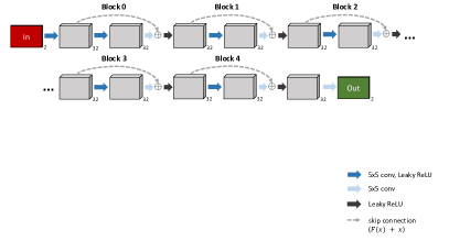
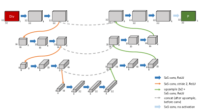
Experiment	Arch.	Layers	Features	Conv. Kernels	Train. Weights
2D Wake Flow B.1	Res-Net	12	32	$5^{2}$	260,354
2D Wake Flow B.1, Small	Sequential	3	32, 64	$5^{2}$	56,898
Buoyancy B.2, MXS	Res-Net	6	4	$5^{2},3^{2}$	1,310
Buoyancy B.2, MS	Res-Net	8	8	$5^{2},3^{2}$	5,114
Buoyancy B.2, Regular	Res-Net	10	16	$5^{2},3^{2}$	35,954
Buoyancy B.2, ML	Res-Net	14	16, 32	$5^{2},3^{2}$	100,114
Buoyancy B.2, MXL	Res-Net	14	32, 64	$5^{2},3^{2}$	400,930
Forced Adv.-diff. B.3	Res-Net	12	32	$5^{2}$	261,154
CG Solver App. B.4	U-Net	22	4, 8, 16, 32	$5^{2}$	127,265
3D Wake Flow B.5	Res-Net	14	24,48	$5^{3},3^{3}$	1,002,411

References

- [1] B. Amos and J. Z. Kolter. OptNet: Differentiable optimization as a layer in neural networks. In International Conference on Machine Learning, 2017.
- [2] V. I. Arnold. Geometrical methods in the theory of ordinary differential equations, volume 250. Springer Science & Business Media, 2012.
- [3] V. Bapst, A. Sanchez-Gonzalez, C. Doersch, K. Stachenfeld, P. Kohli, P. Battaglia, and J. Hamrick. Structured agents for physical construction. In International Conference on Machine Learning, pages 464–474, 2019.
- [4] Y. Bar-Sinai, S. Hoyer, J. Hickey, and M. P. Brenner. Learning data-driven discretizations for partial differential equations. Proceedings of the National Academy of Sciences, 116(31):15344–15349, 2019.
- [5] P. W. Battaglia, J. B. Hamrick, and J. B. Tenenbaum. Simulation as an engine of physical scene understanding. Proceedings of the National Academy of Sciences, 110(45), 2013.
- [6] A. D. Beck, D. G. Flad, and C. Munz. Deep neural networks for data-driven turbulence models. CoRR, abs/1806.04482, 2018.
- [7] M. E. Brachet, D. I. Meiron, S. A. Orszag, B. Nickel, R. H. Morf, and U. Frisch. Small-scale structure of the taylor–green vortex. Journal of Fluid Mechanics, 130:411–452, 1983.
- [8] S. L. Brunton, J. L. Proctor, and J. N. Kutz. Discovering governing equations from data by sparse identification of nonlinear dynamical systems. Proceedings of the National Academy of Sciences, 113(15):3932–3937, 2016.
- [9] T. Q. Chen, Y. Rubanova, J. Bettencourt, and D. K. Duvenaud. Neural ordinary differential equations. In Advances in neural information processing systems, pages 6571–6583, 2018.
- [10] A. J. Chorin. The numerical solution of the navier-stokes equations for an incompressible fluid. Bulletin of the American Mathematical Society, 73(6):928–931, 1967.
- [11] M. Chu and N. Thuerey. Data-driven synthesis of smoke flows with CNN-based feature descriptors. ACM Trans. Graph., 36(4):69:1–69:14, July 2017.
- [12] J. T. Connor, R. D. Martin, and L. E. Atlas. Recurrent neural networks and robust time series prediction. IEEE transactions on neural networks, 5(2):240–254, 1994.
- [13] M. Cranmer, S. Greydanus, S. Hoyer, P. Battaglia, D. Spergel, and S. Ho. Lagrangian neural networks. arXiv:2003.04630, 2020.
- [14] J. P. Crutchfield and B. S. McNamara. Equations of motion from a data series. Complex systems, 1(417-452):121, 1987.
- [15] F. de Avila Belbute-Peres, K. Smith, K. Allen, J. Tenenbaum, and J. Z. Kolter. End-to-end differentiable physics for learning and control. In Advances in neural information processing systems, 2018.
- [16] K. Fukami, K. Fukagata, and K. Taira. Super-resolution reconstruction of turbulent flows with machine learning. Journal of Fluid Mechanics, 870:106–120, 2019.
- [17] S. Ghosal. An analysis of numerical errors in large-eddy simulations of turbulence. Journal of Computational Physics, 125(1):187–206, 1996.
- [18] F. Gibou, D. Hyde, and R. Fedkiw. Sharp interface approaches and deep learning techniques for multiphase flows. Journal of Computational Physics, May 2018.
- [19] G. H. Golub and C. F. Van Loan. Matrix computations, volume 3. JHU press, 2012.
- [20] S. Greydanus, M. Dzamba, and J. Yosinski. Hamiltonian neural networks. In Advances in Neural Information Processing Systems, pages 15353–15363, 2019.
- [21] X. Guo, W. Li, and F. Iorio. Convolutional neural networks for steady flow approximation. In SIGKDD International Conference on Knowledge Discovery and Data Mining, KDD ’16, pages 481–490. ACM, 2016.
- [22] E. Hairer, C. Lubich, and G. Wanner. Geometric numerical integration: structure-preserving algorithms for ordinary differential equations, volume 31. Springer Science & Business Media, 2006.
- [23] K. He, X. Zhang, S. Ren, and J. Sun. Deep residual learning for image recognition. arXiv:1512.03385 [cs], Dec. 2015.
- [24] X. He, H. L. Cao, and B. Zhu. Advectivenet: An eulerian-lagrangian fluidic reservoir for point cloud processing. International Conference on Learning Representations (ICLR), 2020.
- [25] C. R. Henderson. Best linear unbiased estimation and prediction under a selection model. Biometrics, pages 423–447, 1975.
- [26] M. R. Hestenes, E. Stiefel, et al. Methods of conjugate gradients for solving linear systems. Journal of research of the National Bureau of Standards, 49(6):409–436, 1952.
- [27] P. Holl, V. Koltun, and N. Thuerey. Learning to control pdes with differentiable physics. International Conference on Learning Representations (ICLR), 2020.
- [28] J.-T. Hsieh, S. Zhao, S. Eismann, L. Mirabella, and S. Ermon. Learning neural pde solvers with convergence guarantees. arXiv:1906.01200, 2019.
- [29] Y. Hu, L. Anderson, T.-M. Li, Q. Sun, N. Carr, J. Ragan-Kelley, and F. Durand. Difftaichi: Differentiable programming for physical simulation. International Conference on Learning Representations (ICLR), 2020.
- [30] M. Innes, A. Edelman, K. Fischer, C. Rackauckas, E. Saba, V. B. Shah, and W. Tebbutt. A differentiable programming system to bridge machine learning and scientific computing. arXiv 1907.07587, 2019.
- [31] B. M. Johnston, P. R. Johnston, S. Corney, and D. Kilpatrick. Non-newtonian blood flow in human right coronary arteries: steady state simulations. Journal of biomechanics, 37(5):709–720, 2004.
- [32] C. Jones and B. Macpherson. A latent heat nudging scheme for the assimilation of precipitation data into an operational mesoscale model. Meteorological Applications, 4(3):269–277, 1997.
- [33] I. G. Kevrekidis, C. W. Gear, J. M. Hyman, P. G. Kevrekidid, O. Runborg, C. Theodoropoulos, et al. Equation-free, coarse-grained multiscale computation: Enabling mocroscopic simulators to perform system-level analysis. Communications in Mathematical Sciences, 1(4):715–762, 2003.
- [34] B. Kim, V. C. Azevedo, N. Thuerey, T. Kim, M. Gross, and B. Solenthaler. Deep fluids: A generative network for parameterized fluid simulations. Computer Graphics Forum, 2019.
- [35] D. Kingma and J. Ba. Adam: A method for stochastic optimization. arXiv:1412.6980 [cs], Dec. 2014.
- [36] J. N. Kutz. Deep learning in fluid dynamics. Journal of Fluid Mechanics, 814:1–4, 2017.
- [37] Y. Li, H. He, J. Wu, D. Katabi, and A. Torralba. Learning compositional koopman operators for model-based control. arXiv:1910.08264, 2019.
- [38] Y. Li, J. Wu, R. Tedrake, J. B. Tenenbaum, and A. Torralba. Learning particle dynamics for manipulating rigid bodies, deformable objects, and fluids. arXiv:1810.01566, 2018.
- [39] J. Liang, M. Lin, and V. Koltun. Differentiable cloth simulation for inverse problems. In Advances in Neural Information Processing Systems, pages 771–780, 2019.
- [40] Z. Long, Y. Lu, X. Ma, and B. Dong. PDE-Net: Learning PDEs from data. arXiv:1710.09668, 2017.
- [41] M. Magill, F. Qureshi, and H. de Haan. Neural networks trained to solve differential equations learn general representations. In Advances in Neural Information Processing Systems, pages 4071–4081, 2018.
- [42] J. Mathews and R. L. Walker. Mathematical methods of physics, volume 501. WA Benjamin New York, 1970.
- [43] R. Maulik and O. San. A neural network approach for the blind deconvolution of turbulent flows. Journal of Fluid Mechanics, 831:151–181, Oct 2017.
- [44] A. Mohan, D. Daniel, M. Chertkov, and D. Livescu. Compressed convolutional LSTM: An efficient deep learning framework to model high fidelity 3d turbulence. arXiv:1903.00033, 2019.
- [45] J. Morton, A. Jameson, M. J. Kochenderfer, and F. Witherden. Deep dynamical modeling and control of unsteady fluid flows. In Advances in Neural Information Processing Systems, 2018.
- [46] J. M. Murphy, D. M. Sexton, D. N. Barnett, G. S. Jones, M. J. Webb, M. Collins, and D. A. Stainforth. Quantification of modelling uncertainties in a large ensemble of climate change simulations. Nature, 430(7001):768, 2004.
- [47] J.-S. Pang. Error bounds in mathematical programming. Mathematical Programming, 79(1-3):299–332, 1997.
- [48] M. Raissi and G. E. Karniadakis. Hidden physics models: Machine learning of nonlinear partial differential equations. Journal of Computational Physics, 357:125–141, 2018.
- [49] M. Raissi, A. Yazdani, and G. E. Karniadakis. Hidden fluid mechanics: A navier-stokes informed deep learning framework for assimilating flow visualization data. arXiv:1808.04327, 2018.
- [50] B. Rajani, A. Kandasamy, and S. Majumdar. Numerical simulation of laminar flow past a circular cylinder. Applied Mathematical Modelling, 33(3):1228–1247, 2009.
- [51] S. Rasp, P. D. Dueben, S. Scher, J. A. Weyn, S. Mouatadid, and N. Thuerey. Weatherbench: A benchmark dataset for data-driven weather forecasting. arXiv:2002.00469, 2020.
- [52] D. Ray and J. S. Hesthaven. An artificial neural network as a troubled-cell indicator. Journal of Computational Physics, 367:166–191, Aug 2018.
- [53] C. Rhie and W. L. Chow. Numerical study of the turbulent flow past an airfoil with trailing edge separation. AIAA journal, 21(11):1525–1532, 1983.
- [54] O. Ronneberger, P. Fischer, and T. Brox. U-net: Convolutional networks for biomedical image segmentation. In International Conference on Medical Image Computing and Computer-Assisted Intervention, pages 234–241. Springer, 2015.
- [55] A. Sanchez-Gonzalez, J. Godwin, T. Pfaff, R. Ying, J. Leskovec, and P. W. Battaglia. Learning to simulate complex physics with graph networks. arXiv:2002.09405, 2020.
- [56] C. Schenck and D. Fox. Spnets: Differentiable fluid dynamics for deep neural networks. In Conference on Robot Learning, pages 317–335, 2018.
- [57] S. S. Schoenholz and E. D. Cubuk. Jax, md: End-to-end differentiable, hardware accelerated, molecular dynamics in pure python. arXiv:1912.04232, 2019.
- [58] A. Selle, R. Fedkiw, B. Kim, Y. Liu, and J. Rossignac. An unconditionally stable maccormack method. Journal of Scientific Computing, 35(2-3):350–371, June 2008.
- [59] S. Seo, C. Meng, and Y. Liu. Physics-aware difference graph networks for sparsely-observed dynamics. International Conference on Learning Representations (ICLR), 2020.
- [60] J. Sirignano and K. Spiliopoulos. Dgm: A deep learning algorithm for solving partial differential equations. Journal of Computational Physics, 375:1339–1364, 2018.
- [61] J. Stam. Stable fluids. In SIGGRAPH ’99, pages 121–128. ACM, 1999.
- [62] K. Stephan, S. Klink, and C. Schraff. Assimilation of radar-derived rain rates into the convective-scale model cosmo-de at dwd. Quarterly Journal of the Royal Meteorological Society, 134(634):1315–1326, 2008.
- [63] T. F. Stocker, D. Qin, G.-K. Plattner, M. Tignor, S. K. Allen, J. Boschung, A. Nauels, Y. Xia, V. Bex, P. M. Midgley, et al. Climate change 2013: The physical science basis. Contribution of working group I to the fifth assessment report of the intergovernmental panel on climate change, 1535, 2013.
- [64] I. Sutskever, O. Vinyals, and Q. V. Le. Sequence to sequence learning with neural networks. In Advances in neural information processing systems, pages 3104–3112, 2014.
- [65] K. E. Taylor, R. J. Stouffer, and G. A. Meehl. An overview of cmip5 and the experiment design. Bulletin of the American Meteorological Society, 93(4):485–498, 2012.
- [66] N. Thuerey, K. Weißenow, L. Prantl, and X. Hu. Deep learning methods for reynolds-averaged navier–stokes simulations of airfoil flows. AIAA Journal, 58(1):25–36, 2020.
- [67] J. Tompson, K. Schlachter, P. Sprechmann, and K. Perlin. Accelerating eulerian fluid simulation with convolutional networks. In Proceedings of Machine Learning Research, pages 3424–3433, 2017.
- [68] M. Toussaint, K. Allen, K. Smith, and J. B. Tenenbaum. Differentiable physics and stable modes for tool-use and manipulation planning. In Robotics: Science and Systems, 2018.
- [69] B. D. Tracey, K. Duraisamy, and J. J. Alonso. A machine learning strategy to assist turbulence model development. In AIAA aerospace sciences meeting, page 1287, 2015.
- [70] K. Um, X. Hu, and N. Thuerey. Liquid splash modeling with neural networks. Computer Graphics Forum, 37(8):171–182, Dec. 2018.
- [71] B. Ummenhofer, L. Prantl, N. Thuerey, and V. Koltun. Lagrangian fluid simulation with continuous convolutions. In International Conference on Learning Representations, 2020.
- [72] A. Vaswani, N. Shazeer, N. Parmar, J. Uszkoreit, L. Jones, A. N. Gomez, Ł. Kaiser, and I. Polosukhin. Attention is all you need. In Advances in neural information processing systems, pages 5998–6008, 2017.
- [73] W. Wang, S. Axelrod, and R. Gómez-Bombarelli. Differentiable molecular simulations for control and learning. arXiv:2003.00868, 2020.
- [74] N. Watters, D. Zoran, T. Weber, P. Battaglia, R. Pascanu, and A. Tacchetti. Visual interaction networks: Learning a physics simulator from video. In Advances in neural information processing systems, 2017.
- [75] E. Weinan. A proposal on machine learning via dynamical systems. Communications in Mathematics and Statistics, 5(1):1–11, 2017.
- [76] J. Xi, P. Lamata, W. Shi, S. Niederer, S. Land, D. Rueckert, S. G. Duckett, A. K. Shetty, C. A. Rinaldi, R. Razavi, et al. An automatic data assimilation framework for patient-specific myocardial mechanical parameter estimation. In International Conference on Functional Imaging and Modeling of the Heart, pages 392–400. Springer, 2011.
- [77] Y. Xie, E. Franz, M. Chu, and N. Thuerey. tempogan: A temporally coherent, volumetric gan for super-resolution fluid flow. ACM Transactions on Graphics (TOG), 37(4):1–15, 2018.
- [78] J. Zehnder, R. Narain, and B. Thomaszewski. An advection-reflection solver for detail-preserving fluid simulation. ACM Trans. Graph., 37(4):85:1–85:8, July 2018.
- [79] Y. Zhang, W. J. Sung, and D. N. Mavris. Application of convolutional neural network to predict airfoil lift coefficient. Structures, Structural Dynamics, and Materials Conference, 2018.