Momentum Accelerated Multigrid Methods

Abstract

In this paper, we propose two momentum accelerated MG cycles. The main idea is to rewrite the linear systems as optimization problems and apply momentum accelerations, e.g., the heavy ball and Nesterov acceleration methods, to define the coarse-level solvers for multigrid (MG) methods. The resulting MG cycles, which we call them H-cycle (uses heavy ball method) and N-cycle (uses Nesterov acceleration), share the advantages of both algebraic multilevel iteration (AMLI)- and K-cycle (a nonlinear version of the AMLI-cycle). Namely, similar to the K-cycle, our H- and N-cycle do not require the estimation of extreme eigenvalues while the computational cost is the same as AMLI-cycle. Theoretical analysis shows that the momentum accelerated cycles are essentially special AMLI-cycle methods and, thus, they are uniformly convergent under standard assumptions. Finally, we present numerical experiments to verify the theoretical results and demonstrate the efficiency of H- and N-cycle.

65N55, 65F08, 65B99

1 Introduction

Research on multigrid (MG) methods [1, 10, 11] has been very active in recent years. The MG methods are efficient, scalable, and often computationally optimal for solving sparse linear systems of equations arising from discretizations of partial differential equations (PDEs). Therefore, they have been widely used in practical applications [15, 36, 6, 9, 33, 37, 35], especially the algebraic multigrid (AMG) methods [7, 29, 30, 8, 31, 38, 21]. However, the performance and efficiency of MG methods with standard V- or W-cycle may degenerate when the physical and geometric properties of the PDEs become more and more complicated.

For symmetric positive definite (SPD) problems, more involved cycles have been proposed. Axelsson and Vassilevski introduced the algebraic multilevel iteration (AMLI)-cycle MG method [2, 3, 34], which uses Chebyshev polynomial to define the coarse-level solver. However, the AMLI-cycle MG method requires an accurate estimation of extreme eigenvalues on coarse levels to compute the coefficients of the Chebyshev polynomial, which may be difficult in practice. The K-cycle MG method [5, 18], which is a nonlinear version of the AMLI-cycle and does not need to estimate the extreme eigenvalues, was developed thanks to the introduction of the nonlinear preconditioning method [4, 14, 32]. In the K-cycle MG method, $k$ steps of the nonlinear preconditioned conjugate gradient (NPCG) method, with the MG on a coarser level as a preconditioner, are applied to define the coarse-level solver. Under the assumption that the convergence factor of the V-cycle MG with a bounded-level difference is bounded, the uniform convergence property of the K-cycle MG is shown in [18] if $k$ is chosen to be sufficiently large. In [16], a comparative analysis was presented to show that the K-cycle method is always better (or no worse) than the corresponding $k$-fold V-cycle ($k$V-cycle) method. Although the K-cycle method does not need to estimate extreme eigenvalues, its nonlinear nature requires the usage of the NPCG method, which increases the computational and memory cost due to the loss of the three-term recurrence relationship of the standard conjugate gradient (CG) method.

In this work, we propose momentum accelerated MG cycles that have potential to overcome the drawbacks of the AMLI- and K-cycle MG methods. The idea is to rewrite the linear systems on coarse levels as optimization problems and apply the momentum acceleration techniques for optimizations. Two types of accelerations are considered, one is the heavy ball (HB) method [28] and the other one is the Nesterov acceleration (NA) [23, 25, 26]. We use these momentum accelerations to define the coarse-level solvers and the resulting MG cycles are referred to as H-cycle (using the HB method) and N-cycle (using the NA method), respectively. We show that the HB and NA methods, when applied to quadratic optimization problems, can be related to special polynomials approximation. For example, the polynomial associated with the HB method coincides with the best polynomial approximation to $1/x$ proposed in [19, 20]. Thus, H- and N-cycle are essentially special cases of AMLI-cycle. Following standard analysis of the AMLI-cycle, we show that both cycles converge uniformly assuming the extreme eigenvalues are available. The theoretical results are verified numerically when accurate estimations of the extreme eigenvalues are provided.

From our preliminary numerical tests, the H- and N-cycle methods show their efficiency in practice when the extreme eigenvalues (or accurate estimations) are not available. By simply choosing $\lambda_{\max}=1$ and $\lambda_{\min}=0$, the N-cycle MG method shows its superior performance in practice and, surprisingly, is even better than the two-grid method for some cases. N-cycle shares advantages of both AMLI- and K-cycle. Namely, similar to K-cycle, N-cycle does not require the estimation of the extreme eigenvalues while its computational cost is the same as the AMLI-cycle since it is still a linear method. Additionally, since the N-cycle is derived from the optimization point of view, it has the potential to be generalized to other types of problems rather than the SPD problems.

The rest of this paper is organized as follows. In Section 2 we introduce the $k$V-cycle MG algorithm and the HB and NA methods. In Section 3, we present the HB method and NA method for the preconditioned linear system and their relationships with polynomial approximations to $1/x$. Then, the momentum accelerated MG methods and their uniform convergence results are discussed in Section 4. In Section 5, we present some numerical experiments that illustrate the efficiency of momentum accelerated MG methods, especially N-cycle. Finally, some conclusions are drawn in Section 6.

2 Preliminaries

In this section, since our proposed momentum accelerated multigrid methods combine multigrid cycles with momentum accelerations, we first recall the basic multigrid method for solving linear systems, including the $k$V-cycle and AMLI-cycle methods. Then we will review two classical momentum accelerated gradient descent methods, i.e., the HB and NA methods, for solving general unconstrained convex optimization problems.

2.1 Multigrid

We consider solving the following linear system

(1) $$A\mathbf{x}=\mathbf{b}$$

where $A\in\mathbb{R}^{n\times n}$ is SPD. Assume we have constructed a hierarchical structure of the matrices $A_{\ell}\in\mathbb{R}^{n_{\ell}\times n_{\ell}}$, $\ell=1,2,\cdots,J$, with $A_{1}=A$, the prolongations $P_{\ell}\in\mathbb{R}^{n_{\ell}\times n_{\ell+1}}$, $\ell=1,2,\cdots,J-1$, and the restrictions $R_{\ell}=P_{\ell}^{T}\in\mathbb{R}^{n_{\ell+1}\times n_{\ell}}$, $\ell=1,2,\cdots,J-1$. Here, we assume that $A_{\ell+1}=R_{\ell}A_{\ell}P_{\ell}$, $\ell=1,2,\cdots,J-1$. Furthermore, let $M_{\ell}$ denote the smoother on level $\ell$, such as Jacobi or Gauss-Seidel method. Now we define the $k$V-cycle $B_{\ell}$ on level $\ell$ (more precisely, the action of $B_{\ell}\mathbf{b}$) recursively as shown in Algorithm 1. Note that, when $k=1$ or $k=2$, $k$V-cycle MG becomes the classical V-cycle and W-cycle MG, respectively.

Algorithm 1 $k$V-cycle MG: $B_{\ell}\mathbf{b}$

1:  if $\ell==J$ then

2:     $\mathbf{x}_{\ell}=A_{\ell}^{-1}\mathbf{b}$

3:  else

4:     Presmoothing: $\mathbf{x}_{\ell}\leftarrow M_{\ell}\mathbf{b}$

5:     Restriction: $\mathbf{r}_{\ell+1}=R_{\ell}(\mathbf{b}-A_{\ell}\mathbf{x}_{\ell})$

6:     Coarse-grid correction: set $\mathbf{e}_{\ell+1}=\mathbf{0}$ and repeat $\mathbf{e}_{\ell+1}\leftarrow\mathbf{e}_{\ell+1}+B_{\ell+1}(\mathbf{r}_{\ell+1}-A_{\ell+1}\mathbf{e}_{\ell+1})$ $k$ times

7:     Prolongation: $\mathbf{x}_{\ell}\leftarrow\mathbf{x}_{\ell}+P_{\ell}\mathbf{e}_{\ell+1}$

8:     Postsmoothing: $\mathbf{x}_{\ell}\leftarrow\mathbf{x}_{\ell}+M_{\ell}^{T}(\mathbf{b}-A_{\ell}\mathbf{x}_{\ell})$

9:  end if

10:  $B_{\ell}\mathbf{b}\leftarrow\mathbf{x}_{\ell}$

Next, we recall AMLI-cycle. Several polynomials have been proposed to define the coarse-grid correction, which leads to different AMLI-cycle methods. Here we consider the classical choice, the Chebyshev polynomial. Therefore, we first recall the Chebyshev polynomial $C_{k}(t)$, $k=0,1,...$,

(2) $$C_{k}(t)=2tC_{k-1}(t)-C_{k-2}(t),\ k=2,3,...,\ C_{0}(t)=1,\ C_{1}(t)=t.$$

Denote the condition number of a matrix $A$ by $\kappa(A)$, Algorithm 2 gives the classical Chebyshev semi-iterative method [13].

Algorithm 2 Chebyshev semi-iterative method for preconditioned linear system: $\widehat{B}^{C}$

1:  $\mathbf{x}^{0}$ is the given initial guess and $\mathbf{x}^{1}\leftarrow\mathbf{x}^{0}+B(\mathbf{b}-A\mathbf{x}^{0})$

2:  for $k=1,2,...$ do

3:     $\mathbf{x}^{k+1}\leftarrow\frac{2C_{k}(\frac{1}{\rho})}{\rho C_{k+1}(\frac{1}{\rho})}[\mathbf{x}^{k}-B(A\mathbf{x}^{k}-\mathbf{b})-\mathbf{x}^{k-1}]+\mathbf{x}^{k-1}$, where $\rho=1-\frac{1}{\kappa(BA)}$ and B is the preconditioner

4:  end for

In AMLI-cycle, instead of just repeating coarse-grid correction $k$ times in Algorithm 1, Algorithm 2 is used to define the coarse-level solver. Algorithm 3 summarizes the AMLI-cycle method.

Algorithm 3 AMLI-cycle MG: $B_{\ell}\mathbf{b}$

1:  if $\ell==J$ then

2:     $\mathbf{x_{\ell}}=A_{\ell}^{-1}\mathbf{b}$

3:  else

4:     Presmoothing: $\mathbf{x}_{\ell}\leftarrow M_{\ell}\mathbf{b}$

5:     Coarse-grid correction: $\mathbf{x}_{\ell}\leftarrow\mathbf{x}_{\ell}+P_{\ell}\widehat{B}^{C}_{\ell+1}R_{\ell}(\mathbf{b}-A_{\ell}\mathbf{x}_{\ell})$, where $\widehat{B}^{C}_{\ell+1}$ is implemented as in Algorithm 2 with $B_{\ell+1}$ as the preconditioner for $k$ steps

6:     Postsmoothing: $\mathbf{x}_{\ell}\leftarrow\mathbf{x}_{\ell}+M_{\ell}^{T}(\mathbf{b}-A_{\ell}\mathbf{x}_{\ell})$

7:  end if

8:  $B_{\ell}\mathbf{b}\leftarrow\mathbf{x}_{\ell}$

To implement Algorithm 3 in practice, since Algorithm 2 uses a parameter $\rho$, we need to compute $\rho=1-\frac{1}{\kappa(B_{\ell}A_{\ell})}$ on each level. This means that we need to estimate the smallest eigenvalue $\lambda_{\min}(B_{\ell}A_{\ell})$ and the largest eigenvalue $\lambda_{\max}(B_{\ell}A_{\ell})$ since $\kappa(B_{\ell}A_{\ell})=\frac{\lambda_{\max}(B_{\ell}A_{\ell})}{\lambda_{\min}(B_{\ell}A_{\ell})}$. The overall performance of AMLI-cycle Algorithm 3 depends on the estimation of those extreme eigenvalues. In SPD case, a good estimation for the largest eigenvalue is $\lambda_{\max}(B_{\ell}A_{\ell})=1$, However, a good estimation of the smallest eigenvalue $\lambda_{\min}(B_{\ell}A_{\ell})$ is not a straightforward task. This fact motivates the development of nonlinear AMLI-cycle, i.e., the K-cycle MG method. However, the nonlinear feature makes K-cycle less efficient than AMLI-cycle in practice in terms of computation and storage. Therefore, in this work, we aim to develop linear MG cycles that can take advantages of both AMLI- and K-cycles.

2.2 Momentum Acceleration Methods

In this section, we introduce the momentum acceleration techniques which are essential for our proposed momentum accelerated MG cycles. We consider the heavy ball and the Nesterov acceleration methods. Both of them are the first-order momentum acceleration methods for solving the following unconstrained optimization problem,

(3) $$\min_{\mathbf{x}\in\mathbb{R}^{n}}\mathbf{f}(\mathbf{x}),$$

where $\mathbf{f}:\mathbb{R}^{n}\rightarrow\mathbb{R}$ is a continuously differentiable strongly convex function satisfies

(4) $$\frac{\mu}{2}\|\mathbf{x}-\mathbf{y}\|^{2}\leq\mathbf{f}(\mathbf{x})-\mathbf{f}(\mathbf{y})-(\nabla\mathbf{f}(\mathbf{y}),\mathbf{x}-\mathbf{y})\leq\frac{L}{2}\|\mathbf{x}-\mathbf{y}\|^{2},\ \forall\ \mathbf{x},\mathbf{y}\in\mathbb{R}^{n},$$

with $L>0$ being the Lipschitz constant and $\mu>0$ being the convexity constant. Here $(\cdot,\cdot)$ denotes a generic inner product of $\mathbb{R}^{n}$ and $\|\cdot\|$ denotes the corresponding induced norm.

The optimization problem Eq. 3 is usually solved by the gradient descent (GD) method. Under proper assumptions, GD converges linearly with convergence rate $\frac{L-\mu}{L+\mu}$ [26]. Many algorithms have been developed to accelerate the convergence rate and the HB method is a classical GD method by adding momentum at each iteration [28],

Algorithm 4 Heavy ball method

1:  $\mathbf{x}^{0},\mathbf{x}^{1}$ are given as initial iterates, $\alpha$ and $\beta$ are given parameters

2:  for $k=1,2,...$, do

3:     $\mathbf{x}^{k+1}\leftarrow\mathbf{x}^{k}-\alpha\nabla\mathbf{f}(\mathbf{x}^{k})+\beta(\mathbf{x}^{k}-\mathbf{x}^{k-1})$

4:  end for

Let us denote the minimizer of the optimization problem Eq. 3 by $\mathbf{x}^{*}$, then the next theorem shows that the HB method indeed speeds up the convergence under proper assumptions.

Theorem 2.1 ([28]).

If $\mathbf{f}(\mathbf{x})$ satisfies Eq. 4, let $\alpha=\frac{4}{(\sqrt{L}+\sqrt{\mu})^{2}}$, $\beta=(\frac{\sqrt{L}-\sqrt{\mu}}{\sqrt{L}+\sqrt{\mu}})^{2}$ in Algorithm 4, then the following convergence rate estimate holds,

$$\|\mathbf{x}^{k}-\mathbf{x}^{\ast}\|\leq\frac{\sqrt{L}-\sqrt{\mu}}{2\sqrt{\mu}}\bigg{(}\frac{\sqrt{L}-\sqrt{\mu}}{\sqrt{L}+\sqrt{\mu}}\bigg{)}^{k-1}\|\mathbf{x}^{0}-\mathbf{x}^{\ast}\|.$$

Asymptotically, the convergence rate for the HB method is $\frac{\sqrt{L}-\sqrt{\mu}}{\sqrt{L}+\sqrt{\mu}}$ which improves the convergence rate of the GD method since $\frac{\sqrt{L}-\sqrt{\mu}}{\sqrt{L}+\sqrt{\mu}}\leq\frac{L-\mu}{L+\mu}$ in general.

Another momentum acceleration technique is the so-called Nesterov acceleration [23]. The NA method uses a different momentum and is effective and robust for a wide range of problems [23, 27]. Following [23], the NA method for solving Eq. 3 is presented in Algorithm 5.

Algorithm 5 Nesterov acceleration method

1:  $\mathbf{x}^{0},\mathbf{y}^{0}$ are given as initial iterates and $\beta$ is a given parameter

2:  for $k=1,2,...$ do

3:     $\mathbf{y}^{k}\leftarrow\mathbf{x}^{k-1}-\frac{1}{L}\nabla\mathbf{f}(\mathbf{x}^{k-1})$

4:     $\mathbf{x}^{k}\leftarrow\mathbf{y}^{k}+\beta(\mathbf{y}^{k}-\mathbf{y}^{k-1})$

5:  end for

We recall the convergence results of the NA method Algorithm 5 in the following theorem.

Theorem 2.2 ([26]).

If $\mathbf{f}(\mathbf{x})$ satisfies Eq. 4, let $\beta=\frac{\sqrt{L}-\sqrt{\mu}}{\sqrt{L}+\sqrt{\mu}}$,  Algorithm 5 generates a sequence of points $\{\mathbf{x}^{k}\}_{k=0}^{\infty}$ such that

$$\mathbf{f}(\mathbf{x}^{k})-\mathbf{f}^{*}\leq\left(1-\sqrt{\frac{\mu}{L}}\right)^{k}\bigg{[}\mathbf{f}(\mathbf{x}^{0})-\mathbf{f}^{*}+\frac{\mu}{2}\|\mathbf{x}^{0}-\mathbf{x}^{\ast}\|^{2}\bigg{]},$$

where $\mathbf{f}^{*}=\mathbf{f}(\mathbf{x}^{*})$.

Asymptotically, the NA method’s convergence rate is $1-\sqrt{\frac{\mu}{L}}$ which also improves the convergence rate of the GD method. Here, we only present the NA method for the strongly convex functions which is enough for our purpose since we are considering solving SPD linear systems. In fact, as discussed in [23], the NA method can be applied to convex functions (i.e., $\mu=0$) or even nonconvex cases [24, 12]. This makes the NA method more attractive in practice.

3 Momentum Acceleration Methods for Preconditioned Linear Systems

Since we consider solving linear systems Eq. 1 with MG preconditioners, in this section, we present how to apply heavy ball and Nesterov acceleration to preconditioned linear systems, and this will be used to define the coarse-grid correction in our proposed cycles later. To make the application of the HB and NA methods straightforward, we rewrite solving the linear system Eq. 1 with an SPD preconditioner $B$ as solving the following quadratic optimization problem,

(5) $$\min_{\mathbf{x}\in\mathbb{R}^{n}}\frac{1}{2}(A\mathbf{x},\mathbf{x})_{B}-(\mathbf{b},\mathbf{x})_{B},$$

where $(\mathbf{x},\mathbf{x})_{B}:=(B\mathbf{x},\mathbf{x})$. Now we can derive the HB and NA methods for solving Eq. 5 and discuss their convergence behaviors, respectively. Moreover, similar to the semi-iterative method Algorithm 2, which uses Chebyshev polynomials Eq. 2, we show that the HB and NA methods applied to Eq. 5 can be considered as semi-iterative methods based on different polynomials. Roughly speaking, the HB method is related to the polynomial of best uniform approximation to $1/x$ [20] and the NA method is also related to a polynomial that converges to $1/x$.

3.1 Heavy Ball Method for Preconditioned Linear Systems

We first consider the HB method, applying $k$ steps of the HB method (Algorithm 4) to Eq. 5 leads to Algorithm 6, which is the HB method for solving preconditioned linear systems.

Algorithm 6 Heavy ball method for preconditioned linear systems: $\widehat{B}^{H}$

1:  $\mathbf{x}^{0},\mathbf{x}^{1}$ are given as initial iterates, $\alpha$ and $\beta$ are given parameters

2:  for $i=2,...,k$  do

3:     $\mathbf{x}^{i}\leftarrow\mathbf{x}^{i-1}+\alpha B(\mathbf{b}-A\mathbf{x}^{i-1})+\beta(\mathbf{x}^{i-1}-\mathbf{x}^{i-2})$

4:  end for

Algorithm 6 is essentially a linear iterative method that uses two previous iterates. Therefore, it is a semi-iterative method. Moreover, since it is linear, after $k$ iterations, we associate it with a linear operator $\widehat{B}^{H}$ (a matrix in our case since we consider $\mathbb{R}^{n}$). The convergence of the HB method for the preconditioned linear systems follows directly from the general convergence analysis of the HB method presented in Theorem 2.1. Note that in this case, we have $L=\lambda_{\operatorname{max}}(BA)$ and $\mu=\lambda_{\operatorname{min}}(BA)$ and  the result is presented in the following theorem.

Theorem 3.1.

Let $\alpha=\frac{4}{\left(\sqrt{\lambda_{\operatorname{max}}(BA)}+\sqrt{\lambda_{\operatorname{min}}(BA)}\right)^{2}}$, $\beta=\left(\frac{\sqrt{\lambda_{\operatorname{max}}(BA)}-\sqrt{\lambda_{\operatorname{min}}(BA)}}{\sqrt{\lambda_{\operatorname{max}}(BA)}+\sqrt{\lambda_{\operatorname{min}}(BA)}}\right)^{2}$ in Algorithm 6, then the following convergence estimate holds,

$$\|\mathbf{x}^{k}-\mathbf{x}^{\ast}\|\leq\frac{\kappa(BA)-1}{2}\bigg{(}\frac{\sqrt{\kappa(BA)}-1}{\sqrt{\kappa(BA)}+1}\bigg{)}^{k-1}\|\mathbf{x}^{0}-\mathbf{x}^{\ast}\|.$$

3.1.1 Relationship with the Polynomial Approximation of $1/x$

To better understand Algorithm 6 as a semi-iterative method, we aim to find the underlying polynomial associated with it. To this end, we need to look at how the error propagates and, from Algorithm 6, the error $\mathbf{e}^{k}:=\mathbf{x}^{*}-\mathbf{x}^{k}$ satisfies the following three-term recurrence relationship,

$$\mathbf{e}^{k+1}=(I-\alpha BA)\mathbf{e}^{k}+\beta(\mathbf{e}^{k}-\mathbf{e}^{k-1}).$$

This implies that $\mathbf{e}^{k}=p_{k}(BA)\mathbf{e}^{0}$ where $p_{k}(x)$ is a polynomial of degree at most $k$ and satisfies $p_{k}(0)=1$,

(6) $$p_{k+1}(x)=(1-\alpha x)p_{k}(x)+\beta(p_{k}(x)-p_{k-1}(x)).$$

Rewrite $p_{k}(x)=1-xq_{k-1}(x)$, where $q_{k-1}(x)$ is a polynomial of degree at most $k-1$. Substituting it into Eq. 6, we have the following three-term recurrence relationship of $q_{k}(x)$,

(7) $$q_{k+1}(x)=q_{k}(x)+\alpha[1-xq_{k}(x)]+\beta[q_{k}(x)-q_{k-1}(x)].$$

Actually, if

$$q_{0}(x)=\frac{1}{2\lambda_{\max}(BA)}+\frac{1}{2\lambda_{\min}(BA)},$$

and

$$q_{1}(x)=\frac{1}{\sqrt{\lambda_{\max}(BA)\lambda_{\min}(BA)}}+\frac{1}{2\lambda_{\max}(BA)}+\frac{1}{2\lambda_{\min}(BA)}-\frac{x}{\lambda_{\max}(BA)\lambda_{\min}(BA)},$$

then $q_{k}(x)$ is the polynomial of best approximation of $1/x$ respect to $\|\cdot\|_{\infty}$ norm when $\alpha=\frac{4}{(\sqrt{\lambda_{\max}(BA)}+\sqrt{\lambda_{\max}(BA)})^{2}}$ and $\beta=(\frac{\sqrt{\lambda_{\max}(BA)}-\sqrt{\lambda_{\min}(BA)}}{\sqrt{\lambda_{\max}(BA)}+\sqrt{\lambda_{\min}(BA)}})^{2}$, see [20] for details.

By relating the HB method with the polynomial of the best uniform approximation to $1/x$, we give a different perspective to understand the acceleration mechanism of the HB method. In the next section, we will show that the NA method is also related to polynomial approximation to $1/x$, which emphasizes the strong connection between the momentum acceleration and polynomial approximation to $1/x$.

3.2 Nesterov Acceleration Method for Preconditioned Linear Systems

Now we consider Nesterov acceleration. Applying $k$ steps of the NA method Algorithm 5 to Eq. 5, and eliminating $\mathbf{y}^{k}$ lead to Algorithm 7.

Algorithm 7 NA method for preconditioned linear systems: $\widehat{B}^{N}$

1:  $\mathbf{x}^{0},\mathbf{x}^{1}$ are given as initial iterates and $\beta$ is a given parameter

2:  for $i=2,...,k$ do

3:     $\mathbf{x}^{i}\leftarrow(1+\beta)[\mathbf{x}^{i-1}+\frac{1}{L}B(\mathbf{b}-A\mathbf{x}^{i-1})]-\beta[\mathbf{x}^{i-2}-\frac{1}{L}B(\mathbf{b}-A\mathbf{x}^{i-2})]$

4:  end for

Algorithm 7 shows that the NA method for solving preconditioned linear systems also is a linear iterative method that uses the previous two steps. It takes a weighted average of the previous two updates. Essentially, Algorithm 7 is another semi-iterative method, and, due to its linearity, we associate it with a linear operator (or a matrix) $\widehat{B}^{N}$.

Similarly, based on Theorem 2.2, the convergence of the NA method for the preconditioned linear systems follows directly. Note that $L=\lambda_{\operatorname{max}}(BA)$ and $\mu=\lambda_{\operatorname{min}}(BA)$, the convergence result is presented in Theorem 3.2.

Theorem 3.2.

Choose $\beta=\frac{\sqrt{\lambda_{\operatorname{max}}(BA)}-\sqrt{\lambda_{\operatorname{min}}(BA)}}{\sqrt{\lambda_{\operatorname{max}}(BA)}+\sqrt{\lambda_{\operatorname{min}}(BA)}}$ in Algorithm 7, then the following convergence rate estimate holds,

$$\|\mathbf{x}^{k}-\mathbf{x}^{\ast}\|_{A}^{2}\leq 2\bigg{(}1-\frac{1}{\sqrt{\kappa(BA)}}\bigg{)}^{k}\|\mathbf{x}^{0}-\mathbf{x}^{\ast}\|_{A}^{2}.$$

3.2.1 Relationship with the Polynomial Approximation of $1/x$

Next we show that the NA method is also related to the polynomial approximation of $1/x$ when it is applied to the preconditioned linear systems. To this end, denote the error at the $k$-th step of the NA method as $\mathbf{e}^{k}:=\mathbf{x}^{*}-\mathbf{x}^{k}$ and, from Algorithm 7, it satisfies the following three-term recurrence relationship,

$$\mathbf{e}^{k+1}=(1+\beta)(I-\frac{1}{L}BA)\mathbf{e}^{k}-\beta(I-\frac{1}{L}BA)\mathbf{e}^{k-1}.$$

This implies that $\mathbf{e}^{k}=p_{k}(BA)\mathbf{e}^{0}$ where $p_{k}(x)$ is a polynomial of degree at most $k$ and satisfies $p_{k}(0)=1$,

(8) $$p_{k+1}(x)=(1+\beta)(1-\frac{x}{L})p_{k}(x)-\beta(1-\frac{x}{L})p_{k-1}(x).$$

Rewrite $p_{k}(x)=1-xq_{k-1}(x)$, where $q_{k-1}(x)$ is a polynomial of degree at most $k-1$. Substituting it into (8), we have the following three-term recurrence relationship of $q_{k}(x)$,

(9) $$q_{k+1}(x)=q_{k}(x)+\frac{1}{L}[1-xq_{k}(x)]+\beta(1-\frac{x}{L})[q_{k}(x)-q_{k-1}(x)].$$

From Eq. 9, we have $q_{k}(x)\rightarrow 1/x$ as $k\rightarrow\infty$. Comparing with the polynomial of best uniform approximation to $1/x$ given in [20] (or the polynomial related to the HB method as discussed in Section 3.1, the polynomial associated with the NA method is different although it also converges to $1/x$ as we increase the polynomial degree $k$. In [22], this polynomial was explicitly derived.

3.3 Discussion on Polynomials Associated with Different Methods

To better understand the behavior of the polynomial associated with the NA method and its comparison with Chebyshev polynomial used to define the standard AMLI-cycle Algorithm 3 (i.e., the scaled version of (2)) the polynomial (6) associated with the HB method, we plot them in Fig. 1- Fig. 2 together for different polynomial degree $k$ and different choice of $\lambda_{\min}$ while keeping $\lambda_{\max}=1$. Here, to better illustrate how the error converges to $0$, we choose to look at the polynomial $p_{k}(x)$, which converges to $0$ for all cases instead of $q_{k}(x)$, which converges to $1/x$. We emphasis that they are related by $p_{k}(x)=1-xq_{k-1}(x)$.

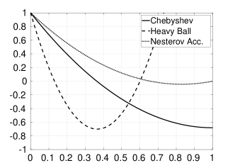
(a) $k=2$

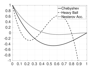
(b) $k=3$

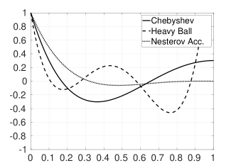
(c) $k=4$

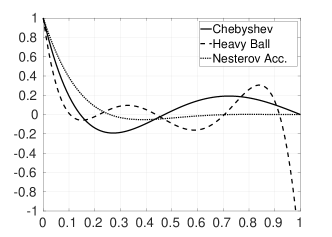
(d) $k=5$

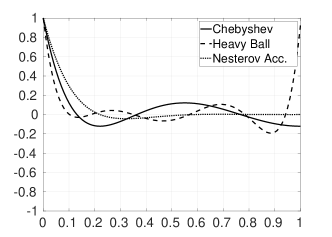
(e) $k=6$

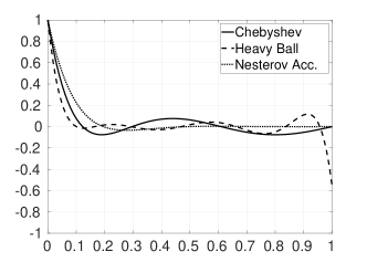
(f) $k=7$

Figure 1: The polynomials $p_{k}(x)$ with $\lambda_{\max}=1,\lambda_{\min}=0.1$ and different $k$.

Fig. 1 shows the case that $\lambda_{\min}=0.1$ and all the polynomials converge to $0$ as we increase the degree $k$. We can also see that on the interval of interest, $[0.1,1]$, all three polynomials give comparable results. The polynomial associated with the HB method usually gives the best results near $0.1$ and the polynomial associated with the NA method usually gives the best results near $1$, while the Chebyshev polynomial gives the best results overall due to its well-known min-max property. This suggests us, in this case, we can use the polynomials associated with the HB and NA methods to define the AMLI-cycle method, and the resulting MG method should have comparable performance with the standard AMLI-cycle method using the Chebyshev polynomial.

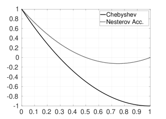
(a) $k=2$

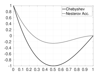
(b) $k=3$

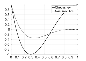
(c) $k=4$

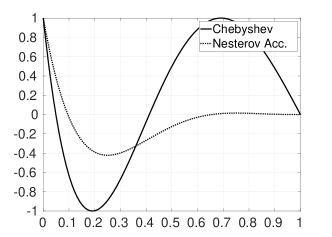
(d) $k=5$

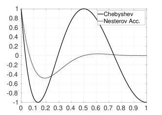
(e) $k=6$

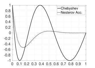
(f) $k=7$

Figure 2: The polynomials $p_{k}(x)$ with $\lambda_{\max}=1,\lambda_{\min}=0$ and different $k$.

However, in practice, estimating $\lambda_{\min}$ might be difficult and expensive. Thus, let us look at the simple choice $\lambda_{\min}=0$. In this case, the polynomial associated with the HB method is not well-defined since neither $q_{0}(x)$ nor $q_{1}(x)$ is well-defined. Therefore, we only plot the other two polynomials in Fig. 2. As we can see, the polynomial associated with the NA methods could provide a better approximation than the Chebyshev methods especially when the polynomial degree $k$ increases. This observation suggests that, in practice, if we replace the Chebyshev polynomial with the polynomial associated with the NA method in AMLI-cycle Algorithm 3, the resulting MG method would be more robust and efficient when we simply choose $\lambda_{\min}=0$. This is verified by our numerical results presented in Section 5.

4 Momentum Accelerated Multigrid Cycles

In this section, we present the momentum accelerated MG cycles. The basic idea is to use $k$ steps of the HB method (Algorithm 6) or the NA method (Algorithm 7) to define the coarse-gird corrections. Since both momentum acceleration methods are semi-iterative methods based on certain polynomials, the resulting MG cycles are essentially special cases of AMLI-cycle. However, to distinguish them from the AMLI-cycle based on Chebyshev polynomials, i.e., Algorithm 3, we call them heavy ball MG cycle (H-cycle) and Nesterov acceleration MG cycle (N-cycle), respectively.

Besides presenting the momentum accelerated MG cycles, we also study their convergence rates by combining the standard analysis of AMLI-cycle and the convergence results in Theorem 3.1 and Theorem 3.2, respectively.

4.1 H-cycle MG Method

In this subsection, we present the H-cycle method, which uses $k$ steps of the heavy ball method (Algorithm 6) to define the coarse-grid correction. Based on the notation introduced in Section 2.1, Algorithm 1, and Algorithm 6, we present the H-cycle MG method in Algorithm 8.

Algorithm 8 H-cycle MG: $B^{H}_{\ell}\mathbf{b}$

1:  if $\ell==J$ then

2:     $\mathbf{x}_{\ell}=A_{\ell}^{-1}\mathbf{b}$

3:  else

4:     Presmoothing: $\mathbf{x}_{\ell}\leftarrow M_{\ell}\mathbf{b}$

5:     Coarse-grid correction: $\mathbf{x}_{\ell}\leftarrow\mathbf{x}_{\ell}+P_{\ell}\widehat{B}^{H}_{\ell+1}R_{\ell}(\mathbf{b}-A_{\ell}\mathbf{x}_{\ell})$, where $\widehat{B}^{H}_{\ell+1}$ is implemented as in Algorithm 6 with $B^{H}_{\ell+1}$ as the preconditioner for $k$ steps

6:     Postsmoothing: $\mathbf{x}_{\ell}\leftarrow\mathbf{x}_{\ell}+M_{\ell}^{T}(\mathbf{b}-A_{\ell}\mathbf{x}_{\ell})$

7:  end if

8:  $B^{H}_{\ell}\mathbf{b}\leftarrow\mathbf{x}_{\ell}$

As mentioned before, H-cycle is essentially an AMLI-cycle MG method. Moreover, since the polynomial Eq. 7 associated with the HB method is the polynomial of best uniform approximation to $1/x$, therefore our H-cycle is equivalent to the AMLI-cycle method proposed in [19] and the estimate of the condition number has been analyzed in [19] as well. Here, to give a more intuitively expression, following standard analysis for the AMLI-cycle method presented in [35] and utilizing the convergence theory of the HB method (Theorem 3.1), we will show that H-cycle MG method presented in Algorithm 8 provides a uniform preconditioner under the assumption that the condition number of the two-grid method $\kappa_{TG}$ is uniformly bounded. We summarize the results in Theorem 4.1 and comment that the general case can be analyzed similarly when the conditioned number of the V-cycle MG method with a bounded-level difference is uniformly bounded.

Theorem 4.1.

Let $B^{H}_{\ell}$ be defined by Algorithm 8 and $\widehat{B}^{H}_{\ell}$ be implemented as in Algorithm 6 with $B^{H}_{\ell}$ as the preconditioner with $\alpha=\frac{4}{\left(\sqrt{\lambda_{\operatorname{max}}(B^{H}_{\ell}A_{\ell})}+\sqrt{\lambda_{\operatorname{min}}(B^{H}_{\ell}A_{\ell})}\right)^{2}}$ and $\beta=\left(\frac{\sqrt{\lambda_{\operatorname{max}}(B^{H}_{\ell}A_{\ell})}-\sqrt{\lambda_{\operatorname{min}}(B^{H}_{\ell}A_{\ell})}}{\sqrt{\lambda_{\operatorname{max}}(B^{H}_{\ell}A_{\ell})}+\sqrt{\lambda_{\operatorname{min}}(B^{H}_{\ell}A_{\ell})}}\right)^{2}$. Assume that the two-grid method has uniformly bounded condition number $\kappa_{TG}$, then the condition number of $B^{H}_{\ell}A_{\ell}$ can be uniformly bounded. More specifically, we can choose $\delta\in[0,1)$ and $k\in\mathbb{N}$, satisfying

(10) $$2(1-\delta)(1+\sqrt{1-\delta})^{k-1}-\delta(1-\sqrt{1-\delta})^{k-1}>0,$$

such that

(11) $$(1-\delta)\kappa_{TG}+\kappa_{TG}\frac{\delta(1-\delta)(1-\sqrt{1-\delta})^{k-1}}{2(1-\delta)(1+\sqrt{1-\delta})^{k-1}-\delta(1-\sqrt{1-\delta})^{k-1}}\leq 1.$$

Then we have the following uniform estimate for the H-cycle preconditioner $B^{H}_{\ell}$ defined by Algorithm 8,

(12) $$\mathbf{x}^{T}A_{\ell}\mathbf{x}\leq\mathbf{x}^{T}(B^{H}_{\ell})^{-1}\mathbf{x}\leq\frac{1}{1-\delta}\mathbf{x}^{T}A_{\ell}\mathbf{x}$$

Proof 4.2.

First of all, it is clear that, as $\delta\rightarrow 1$, the left-hand side of Eq. 11 tends to $0$ , which implies that there exists a $\delta$ satisfies Eq. 11.

In order to proof the inequality Eq. 12, assume by induction that $1-\delta\leq\frac{1}{1+\delta_{\ell+1}}$, where the eigenvalue of $B^{H}_{\ell+1}A_{\ell+1}$ are in the interval $[\frac{1}{1+\delta_{\ell+1}},1]$ for some $\delta_{\ell+1}\geq 0$. Then we want to show that the eigenvalues of $B^{H}_{\ell}A_{\ell}$ are contained in an interval $[\frac{1}{1+\delta_{\ell}},1]$ for some $\delta_{\ell}\geq 0$. Since we use $k$ steps of Algorithm 6 with $B^{H}_{\ell}$ as a preconditioner to define $\widehat{B}^{H}_{\ell}$ in Algorithm 8, we have that

$$\lambda(\widehat{B}^{H}_{\ell+1}A_{\ell+1})\in\left[\frac{1}{1+\widetilde{\delta}_{\ell+1}},1\right]$$

where

$$\widetilde{\delta}_{\ell+1}=\sup\left\{\frac{1}{1-p_{k}(x)}-1,x\in\left[\frac{1}{1+\delta_{\ell+1}},1\right]\right\}\leq\sup\left\{\frac{p_{k}(x)}{1-p_{k}(x)},x\in[1-\delta,1]\right\},$$

and $p_{k}$ is the polynomial defined by Eq. 6. According to Theorem 3.1, we have

$$p_{k}(x) \leq\frac{\kappa(B_{\ell+1}^{H}A_{\ell+1})-1}{2}\left(\frac{\sqrt{\kappa(B_{\ell+1}^{H}A_{\ell+1})}-1}{\sqrt{\kappa(B_{\ell+1}^{H}A_{\ell+1})}+1}\right)^{k-1}$$

$$\leq\frac{\delta}{2(1-\delta)}\left(\frac{1-\sqrt{1-\delta}}{1+\sqrt{1-\delta}}\right)^{k-1},\quad\forall\ x\in[1-\delta,1],$$

then we have‘$0\leq p<1$ for all $x\in[1-\delta,1]$ due to the choice of $k$. Because $\frac{t}{(1-t)}$ is an increasing function of $t\in[0,1)$, we have

$$\widetilde{\delta}_{\ell+1} \leq\displaystyle{\frac{\sup\left\{p_{k}(x),x\in[1-\delta,1]\right\}}{1-\sup\{p_{k}(x),x\in[1-\delta,1]\}}}$$

$$=\displaystyle{\frac{\delta(1-\sqrt{1-\delta})^{k-1}}{2(1-\delta)(1+\sqrt{1-\delta})^{k-1}-\delta(1-\sqrt{1-\delta})^{k-1}}}.$$

On the other hand, use Corollary 5.11 in [35], we have $1+\delta_{\ell}\leq(1+\widetilde{\delta}_{\ell+1})\kappa_{TG}$. Therefore, in order to confirm the induction assumption, we need to choose $\delta$ such that $1+\delta_{\ell}\leq(1+\widetilde{\delta}_{\ell+1})\kappa_{TG}\leq\frac{1}{1-\delta}$, which is

$$\begin{array}[]{l}\displaystyle{\kappa_{TG}\left[1+\frac{\delta(1-\sqrt{1-\delta})^{k-1}}{2(1-\delta)(1+\sqrt{1-\delta})^{k-1}-\delta(1-\sqrt{1-\delta})^{k-1}}\right]\leq\frac{1}{1-\delta}}.\end{array}$$

This inequality is equivalent to Eq. 11. On the other hand, under the assumption of Eq. 10, it is obviously that

$$\begin{array}[]{l}\displaystyle{\kappa_{TG}\left[1+\frac{\delta(1-\sqrt{1-\delta})^{k-1}}{2(1-\delta)(1+\sqrt{1-\delta})^{k-1}-\delta(1-\sqrt{1-\delta})^{k-1}}\right]\geq 1}.\end{array}$$

Thus, this completes the proof of Eq. 12.

Remark 4.3.

Theorem 4.1 shows that H-cycle provides a uniform preconditioner under the assumption that the condition number of the two-grid method $\kappa_{TG}$ is bounded. When $k=2$, we have $\delta\in[0,2\sqrt{2}-2)$ from Eq. 10. Note that the convergence factor $\delta_{TG}=1-1/\kappa_{TG}$, inequality Eq. 11 reduces to

$$(1-\delta)+\frac{\delta(1-\delta)(1-\sqrt{1-\delta})}{2(1-\delta)(1+\sqrt{1-\delta})-\delta(1-\sqrt{1-\delta})}=\frac{1}{\kappa_{TG}}=1-\delta_{TG}.$$

This implies that $\delta_{TG}\in(0,0.5464)$, which means that, if the two-grid method at any level $\ell$ (with exact solution at coarse level $\ell+1$ has a uniformly bounded convergence factor $\delta_{TG}<0.5464$, then the corresponding H-cycle has a uniformly bounded convergence factor $\delta$. Obviously, it is better than W-cycle ($2$-fold V-cycle), because, for W-cycle to be uniformly convergent, the convergence factor of the two-grid method should be bounded to be $\delta_{TG}<0.5$ (See Corollary 5.30 in [35]).

4.2 N-cycle MG Method

Similarly, our proposed the N-cycle MG method uses $k$ steps of the NA method Algorithm 7 to define the coarse-level solvers. Based on the notation introduced in Section 2.1, Algorithm 1, and Algorithm 7, Algorithm 9 presents the N-cycle algorithm recursively.

Algorithm 9 N-cycle MG: $B^{N}_{\ell}\mathbf{b}$

1:  if $\ell==J$ then

2:     $\mathbf{x}_{\ell}=A_{\ell}^{-1}\mathbf{b}$

3:  else

4:     Presmoothing: $\mathbf{x}_{\ell}\leftarrow M_{\ell}\mathbf{b}$

5:     Coarse-grid correction: $\mathbf{x}\leftarrow\mathbf{x}_{\ell}+P_{\ell}\widehat{B}^{N}_{\ell+1}R_{\ell}(\mathbf{b}-A_{\ell}\mathbf{x}_{\ell})$, where $\widehat{B}^{N}_{\ell+1}$ is implemented as in Algorithm 7 with $B^{N}_{\ell+1}$ as the preconditioner for $k$ steps

6:     Postsmoothing: $\mathbf{x}_{\ell}\leftarrow\mathbf{x}_{\ell}+M_{\ell}^{T}(\mathbf{b}-A_{\ell}\mathbf{x}_{\ell})$

7:  end if

8:  $B^{N}_{\ell}\mathbf{b}\leftarrow\mathbf{x}_{\ell}$

The N-cycle MG method can be viewed as an AMLI-cycle method using the polynomial defined in Eq. 9. Following standard analysis of the AMLI-cycle method presented in [35] and utilizing the convergence theory of the NA method (Theorem 3.2), we can show that N-cycle MG method presented in Algorithm 9 provides a uniform preconditioner under the assumption that the condition number of the two-grid method $\kappa_{TG}$ is uniformly bounded. We summarize the results in Theorem 4.4 and comment that the general case ban analyzed similarly when the conditioned number of the V-cycle MG method with a bounded-level difference is uniformly bounded.

Theorem 4.4.

Let $B^{N}_{\ell}$ be defined by Algorithm 9 and $\widehat{B}^{N}_{\ell}$ be implemented as in Algorithm 7 wit  $B^{N}_{\ell}$ as the preconditioner with $\beta=\frac{\sqrt{\lambda_{\operatorname{max}}(B^{N}_{\ell}A_{\ell})}-\sqrt{\lambda_{\operatorname{min}}(B^{N}_{\ell}A_{\ell})}}{\sqrt{\lambda_{\operatorname{max}}(B^{N}_{\ell}A_{\ell})}+\sqrt{\lambda_{\operatorname{min}}(B^{N}_{\ell}A_{\ell})}}$. Assume that the two-grid method has a uniformly bounded condition number $\kappa_{TG}$, then the condition number of $B^{N}_{\ell}A_{\ell}$ can be uniformly bounded. More specifically, there exists $\delta\in[0,1)$ and $k\in\mathbb{N}$, satisfying $2(1-\sqrt{1-\delta})^{k}<1$, such that

(13) $$(1-\delta)\kappa_{TG}+\kappa_{TG}\frac{(1-\delta)\sqrt{2(1-\sqrt{1-\delta})^{k}}}{1-\sqrt{2(1-\sqrt{1-\delta})^{k}}}\leq 1.$$

And we have the following uniform estimate for the N-cycle method $B^{N}_{\ell}$ defined by Algorithm 9,

(14) $$\mathbf{x}^{T}A_{\ell}\mathbf{x}\leq\mathbf{x}^{T}(B^{N}_{\ell})^{-1}\mathbf{x}\leq\frac{1}{1-\delta}\mathbf{x}^{T}A_{\ell}\mathbf{x}.$$

Proof 4.5.

The proof is essentially the same as the proof of Theorem 4.1. The only two differences are, the polynomial $p_{k}(x)$ used here is the one defined by Eq. 8, and the corresponding convergence property is that presented in Theorem 3.2.

More precisely, since we use $k$ steps of Algorithm 7 with $B^{N}_{\ell}$ as a preconditioner to define $\widehat{B}^{N}_{\ell}$ in  Algorithm 9, we have that the eigenvalues of $\widehat{B}^{N}_{\ell+1}A_{\ell+1}$ are contained in the interval $[\frac{1}{1+\widetilde{\delta}_{\ell+1}},1]$, where

$$\begin{array}[]{l}\widetilde{\delta}_{\ell+1}=\displaystyle{\sup\left\{\frac{1}{1-p_{k}(x)}-1,x\in[\frac{1}{1+\delta_{\ell+1}},1]\right\}}\leq\displaystyle{\sup\left\{\frac{p_{k}(x)}{1-p_{k}(x)},x\in[1-\delta,1]\right\}},\\ \end{array}$$

and $p_{k}(x)$ is the polynomial defined by Eq. 8. According to Theorem 3.2, we have

$$p_{k}^{2}(x)\leq 2\left(1-\frac{1}{\sqrt{\kappa(B^{N}_{\ell+1}A_{\ell+1})}}\right)^{k}\leq 2\left(1-\sqrt{1-\delta}\right)^{k},\ \forall\ x\in[1-\delta,1],$$

then $p_{k}^{2}(x)<1$ for all $x\in[1-\delta,1]$ due to the choice of $k$. Because $\frac{t}{(1-t)}$ is an increasing function of $t\in(-1,1)$, we have

$$\begin{array}[]{l}\widetilde{\delta}_{\ell+1}\leq\displaystyle{\frac{\sup\left\{p_{k}(x),x\in[1-\delta,1]\right\}}{1-\sup\{p_{k}(x),x\in[1-\delta,1]\}}}=\displaystyle{\frac{\sqrt{2\left(1-\sqrt{1-\delta}\right)^{k}}}{1-\sqrt{2\left(1-\sqrt{1-\delta}\right)^{k}}}}.\end{array}$$

On the other hand, use Corollary 5.11 in [35], we have $1+\delta_{\ell}\leq(1+\widetilde{\delta}_{\ell+1})\kappa_{TG}$. Therefore, in order to confirm the induction assumption, we need to choose $\delta$ such that $1+\delta_{\ell}\leq(1+\widetilde{\delta}_{\ell+1})\kappa_{TG}\leq\frac{1}{1-\delta}$, which is

$$\begin{array}[]{l}\displaystyle{\kappa_{TG}\left[1+\frac{\sqrt{2\left(1-\sqrt{1-\delta}\right)^{k}}}{1-\sqrt{2\left(1-\sqrt{1-\delta}\right)^{k}}}\right]\leq\frac{1}{1-\delta}}.\end{array}$$

This inequality is equivalent to Eq. 13. On the other hand, under the assumption that $2(1-\sqrt{1-\delta})^{k}<1$, it is obviously that

$$\begin{array}[]{l}(1+\widetilde{\delta}_{\ell+1})\kappa_{TG}=\displaystyle{\kappa_{TG}\left[1+\frac{\sqrt{2\left(1-\sqrt{1-\delta}\right)^{k}}}{1-\sqrt{2\left(1-\sqrt{1-\delta}\right)^{k}}}\right]}\geq 1.\end{array}$$

Thus, this completes the proof of Eq. 14.

Next, we provide several remarks to better interpret the theoretical results of Theorem 4.4, comparison with standard AMLI-cycle, and limitations in predicting the performance of the N-cycle method in practice.

Remark 4.6.

When $k=2$, we have $\delta\in[0,\sqrt{2}-1/2)$ due to $2(1-\sqrt{1-\delta})^{2}<1$. Note that the convergence factor of the two-grid method satisfies $\delta_{TG}=1-1/\kappa_{TG}$, inequality Eq. 13 reduces to

$$(1-\delta)+\frac{\sqrt{2}(1-\delta)(1-\sqrt{1-\delta})}{1-\sqrt{2}(1-\sqrt{1-\delta})}=\frac{1}{\kappa_{TG}}=1-\delta_{TG}.$$

This implies that $\delta_{TG}\in(0,0.7071)$, which means that, if the two-grid method at any level $\ell$ (with exact solution at coarse level $\ell+1$) has a uniformly bounded convergence factor $\delta_{TG}<0.7071$, then the corresponding N-cycle has a uniformly bounded convergence factor $\delta$. It is better than W-cycle ($2$-fold V-cycle) because, for W-cycle to be uniformly convergent, the convergence factor of the two-grid method should be bounded to be $\delta_{TG}<0.5$ (See Corollary 5.30 in [35]).

Remark 4.7.

If we want AMLI-cycle using Chebyshev polynomial Eq. 2 (i.e., Algorithm 3) to be uniformly convergent, the convergence factor of the two-grid method should be $\delta_{TG}<0.75$, which is slightly better than N-cycle theoretically due to the min-max property of the Chebyshev polynomials. However, it is a theoretical result based on the assumption that the extreme eigenvalues of the MG preconditioned coarse-level problems are available, which could be quite expensive or even impossible in practice. As we will see from our numerical experiments in Section 5, we can simply use the estimations $\lambda_{\operatorname{max}}=1$ and $\lambda_{\operatorname{min}}=0$, i.e., $\beta=1$, to define the N-cycle method in practice and still obtain a good performance. Moreover, the N-cycle MG method could outperform the AMLI-cycle in practice with such a simple choice of the parameter $\beta=1$.

5 Numerical Results

In this section, we present some numerical experiments to illustrate the efficiency of the N-cycle MG method. In our numerical experiments, we discretize all the examples using the linear finite-element method on uniform triangulations of the domain $\Omega$ with mesh size $h$. Namely, the matrix $A$ in (1) is the stiffness matrix of the finite-element discretizations. The true solution of the linear system is $\mathbf{x}=[1,2,...,N]^{T}\mathbf{R}^{N}$, $N=1/h$, and the right hand side $\mathbf{b}$ is computed accordingly for all the examples. We use the unsmoothed aggregation AMG (UA-AMG) method [17] in all the experiments since it is well-known that, the V-cycle UA-AMG method does not converge uniformly in general and more involved cycles are needed. For all the MG cycles, we use Gauss-Seidel (GS) smoother ($1$ step forward GS for pre-smoothing and $1$ step backward GS for post-smoothing). In our implementations of Algorithm 6 (used in H-cycle Algorithm 8) and Algorithm 7 (used in N-cycle Algorithm 9), we choose $\mathbf{x}^{0}=0$ and $\mathbf{x}^{1}=\frac{(B\mathbf{b},B\mathbf{b})}{(B\mathbf{b},B\mathbf{b})_{A}}B\mathbf{b}$ (i.e., one step of steepest descent method for solving (5) with $\mathbf{x}^{0}=0$). We always use $\lambda_{\max}=1$ (which is a good estimation for SPD problems in general) and choose different $\lambda_{\min}$ to test the performance. In all the numerical experiments, all the MG methods are used as stand-alone iterative solvers. We use zero initial guess and the stopping criteria is that the relative residual is less than or equal to $10^{-12}$. Besides the number of iterations to convergence, the average convergence factor of the last five iterations is reported to illustrate the performance of the MG methods.

Example 5.1.

Consider the model problem on $\Omega=[0,1]\times[0,1]$.

$$\begin{array}[]{rcl}-\Delta\mathbf{u}&=&\mathbf{f},\ \ \ \text{in}\ \ \Omega,\\ \mathbf{u}&=&0,\ \ \ \text{on}\ \ \partial\Omega.\end{array}$$

Table 1: Convergence factors (and number of iterations to convergence) for different MG cycles on Example 5.1. (“-” means the method diverges)

	$h=1/64$	$h=1/128$	$h=1/256$	$h=1/512$
	Two-grid
	0.502005 (34)	0.503784 (34)	0.505978 (35)	0.505159 (35)
	$k$V-cycle
$k=1$	0.804198 (109)	0.841594 (129)	0.856977 (135)	0.862513 (133)
$k=2$	0.703505 (67)	0.744310 (77)	0.763329 (79)	0.763709 (77)
$k=3$	0.639391 (63)	0.677776 (58)	0.692216 (59)	0.690056 (58)
	K-cycle
$k=2$	0.514746 (38)	0.521637 (38)	0.525396 (39)	0.526877 (39)
$k=3$	0.513212 (36)	0.517616 (36)	0.518201 (36)	0.518781 (36)
	AMLI-cycle (estimate $\lambda_{\min}$)
$k=2$	0.369682 (19)	0.417879 (21)	0.406392 (20)	0.421880 (20)
$k=3$	0.404490 (21)	0.420391 (22)	0.439241 (21)	0.396547 (24)
	AMLI-cycle ($\lambda_{\min}=0$)
$k=2$	0.369628 (19)	0.417948 (21)	0.406392 (20)	0.421880 (20)
$k=3$	0.305806 (21)	0.318781 (22)	0.310708 (21)	0.323530 (22)
	H-cycle (estimate $\lambda_{\min}$)
$k=2$	0.531629 (38)	0.545223 (39)	0.550238 (38)	0.541994 (37)
$k=3$	0.498365 (34)	0.501108 (34)	0.497384 (34)	0.494567 (33)
	H-cycle ($\lambda_{\min}=0.1$ )
$k=2$	0.495479 (34)	0.519374 (35)	0.528661 (36)	0.526969 (35)
$k=3$	0.477346 (31)	0.491798 (32)	0.490162 (33)	0.492058 (32)
	H-cycle ($\lambda_{\min}=0$)
$k=2$	0.260674 (16)	0.314143 (17)	0.214169 (16)	0.192636 (16)
$k=3$	-	-	-	-
	N-cycle (estimate $\lambda_{\min}$)
$k=2$	0.484492 (35)	0.489757 (36)	0.490731 (36)	0.491870 (35)
$k=3$	0.482751 (34)	0.481927 (34)	0.476483 (34)	0.476189 (33)
	N-cycle ($\lambda_{\min}=0$)
$k=2$	0.407385 (29)	0.416979 (29)	0.417469 (29)	0.420126 (29)
$k=3$	0.391101 (25)	0.390428 (25)	0.394326 (26)	0.388651 (25)

In Table 1, we show the convergence factor and number of iterations of different MG cycles when the mesh size $h=1/64,1/128,1/256,1/512$. As we can see, although the two-grid method achieves uniform convergence, the performance of the V-cycle (i.e., $k$V-cycle with $k=1$) degenerates as expected since we use the UA-AMG method. Because the convergence factor of Two-grid is slightly larger than $0.5$, W-cycle (i.e., $k$V-cycle with $k=2$) still does not converge uniformly as both the convergence factor and the number of iterations grow as $h$ gets smaller. $k$V-cycle becomes uniformly convergent when $k=3$. The K- and AMLI-cycle methods, which are designed for this case, all achieve uniform convergence when $k=2$. For the proposed H- and N-cycle, when we estimate $\lambda_{\min}$ on each level to compute the parameters used in the HB and NA method, we obtain uniform convergence. This confirms the theoretical results Theorem 4.1 and Theorem 4.4.

As we mentioned, estimating $\lambda_{\min}$ might be difficult and expensive in practice. Therefore, we investigate the performances of AMLI-, H-, and N-cycle when simply choose $\lambda_{\min}=0$. As shown in Table 1, while all three cycles converge nicely when $k=2$, H-cycle diverges when $k=3$. In fact, it diverges for $k\geq 3$. This is because the HB method, which is used to define H-cycle, was developed for strongly convex functions, and the choice $\lambda_{\min}=0$ only implies convexity. Once we choose $\lambda_{\min}=0.1>0$, H-cycle converges uniformly again. On the other hand, for the simple choice $\lambda_{\min}=0$, the N-cycle method not only achieves uniform convergence but also outperforms the $k$V-cycle, K-cycle, and, surprisingly, even two-grid method, which demonstrates its efficiency in practice.

From Table 1, we notice that AMLI-cycle Algorithm 3 with simple choice $\lambda_{\min}=0$ also performs quite well, even better than N-cycle, when $k=2$ or $3$. However, our investigation in Section 3.3 shows that it is not the case when we increase $k$, which is confirmed by the numerical results presented in Table 2. When $k$ increases, AMLI-cycle’s performance deteriorates due to the lack of accurate estimation of $\lambda_{\min}$. In contrast, H-cycle with $\lambda_{\min}=0.1$ and N-cycle with $\lambda_{\min}=0$ converge uniformly when $k$ increases. In practice, considering the trade-off between the performance (fast convergence and robustness with respect to parameters) and the efficiency (low computational and storage cost), we would recommend using N-cycle with $\lambda_{\min}=0$ and $k=2$ or $3$.

Table 2: Convergence factors (and number of iterations to convergence) for the AMLI-, H- and N-cycle with fixed $\lambda_{\min}$ on Example 5.1

	$h=1/64$	$h=1/128$	$h=1/256$	$h=1/512$
	AMLI-cycle method ($\lambda_{\min}=0$)
$k=4$	0.743668 (88)	0.925038 (329)	0.980392 (999)	0.995041 (999)
$k=5$	0.751663 (92)	0.766853 (96)	0.801483 (113)	0.776317 (101)
$k=6$	0.852902 (144)	0.855592 (142)	0.869571 (158)	0.881878 (155)
$k=7$	0.922309 (297)	0.946864 (422)	0.958507 (503)	0.965900 (679)
	H-cycle method ($\lambda_{\min}=0.1$)
$k=4$	0.497761 (35)	0.497349 (35)	0.502591 (36)	0.498534 (35)
$k=5$	0.495767 (34)	0.494605 (34)	0.500665 (35)	0.497057 (34)
$k=6$	0.511109 (35)	0.513025 (35)	0.514338 (36)	0.514755 (35)
$k=7$	0.524589 (37)	0.507319 (35)	0.509050 (35)	0.508896 (35)
	N-cycle method ($\lambda_{\min}=0$)
$k=4$	0.395807 (26)	0.417665 (27)	0.406770 (27)	0.404306 (26)
$k=5$	0.440458 (29)	0.451704 (30)	0.452052 (30)	0.445281 (30)
$k=6$	0.482864 (33)	0.489894 (33)	0.496542 (34)	0.492264 (34)
$k=7$	0.502005 (34)	0.537300 (38)	0.544519 (38)	0.540128 (38)

Example 5.2.

The second model problem is a diffusion equation with jump coefficient on $\Omega=[0,1]\times[0,1]$,

$$\begin{array}[]{rcl}-\nabla\cdot(a(\mathbf{x})\nabla\mathbf{u})&=&\mathbf{f},\ \ \ \text{in}\ \ \Omega,\\ \mathbf{u}&=&0,\ \ \ \text{on}\ \ \partial\Omega,\end{array}$$

where $a(\mathbf{x})=1$ in $[0.25,0.5]\times[0.25,0.5]\cup[0.5,0.75]\times[0.5,0.75]$ and $a(\mathbf{x})=10^{-6}$ everywhere else.

Table 3: Convergence factors (and number of iterations to convergence) for different MG cycles on Example 5.2. (“-” means the method diverges)

	$h=1/64$	$h=1/128$	$h=1/256$	$h=1/512$
	Two-grid method
	0.533777 (44)	0.524908 (43)	0.555066 (45)	0.543575 (45)
	k-fold V-cycle method
$k=1$	0.762328 (101)	0.827267 (141)	0.860452 (187)	0.902543 (202)
$k=2$	0.673176 (69)	0.723526 (87)	0.782840 (110)	0.802340 (115)
$k=3$	0.617277 (57)	0.669389 (68)	0.728067 (83)	0.730747 (86)
	K-cycle method
$k=2$	0.529076 (44)	0.524365 (43)	0.534955 (44)	0.528044 (44)
$k=3$	0.534470 (44)	0.529453 (43)	0.533266 (44)	0.530886 (44)
	AMLI-cycle method (estimate $\lambda_{\min}$)
$k=2$	0.432465 (33)	0.420315 (32)	0.461580 (35)	0.447631 (35)
$k=3$	0.451159 (34)	0.430807 (33)	0.470242 (37)	0.463407 (36)
	AMLI-cycle method ($\lambda_{\min}=0$)
$k=2$	0.432465 (33)	0.420315 (32)	0.461580 (35)	0.447631 (35)
$k=3$	0.430666 (30)	0.368431 (28)	0.408762 (31)	0.403546 (31)
	H-cycle method (estimate $\lambda_{\min}$)
$k=2$	0.567908 (48)	0.569448 (49)	0.613660 (55)	0.591049 (50)
$k=3$	0.528280 (43)	0.515659 (42)	0.530545 (44)	0.527500 (43)
	H-cycle method ($\lambda_{\min}=0.1$)
$k=2$	0.525578 (43)	0.535880 (45)	0.598752 (52)	0.595025 (51)
$k=3$	0.517179 (41)	0.501953 (40)	0.539879 (44)	0.543111 (43)
	H-cycle method ($\lambda_{\min}=0$)
$k=2$	0.365756 (28)	0.333696 (26)	0.359729 (28)	0.349733 (27)
$k=3$	-	-	-	-
	N-cycle method (estimate $\lambda_{\min}$)
$k=2$	0.518716 (42)	0.507191 (41)	0.513673 (42)	0.497285 (40)
$k=3$	0.524168 (42)	0.499282 (41)	0.506174 (41)	0.475311 (38)
	N-cycle method ($\lambda_{\min}=0$)
$k=2$	0.469765 (36)	0.430731 (33)	0.436282 (34)	0.427501 (33)
$k=3$	0.485852 (36)	0.421445 (32)	0.449840 (33)	0.413262 (31)

We present the convergence factors and the number of iterations of different MG cycles for Example 5.2 in Table 3. We can see that the two-grid method converges uniformly, however, since we use the UA-AMG method and the problem has a large jump in the coefficient, the performance of the V-cycle (i.e., $k$V-cycle with $k=1$) degenerates as expected. In fact, the $k$V-cycle still does not converge uniformly with respect to $h$ when $k=2$ or $3$. The K- and AMLI-cycle methods achieve uniform convergence when $k=2$ and $3$. For the H- and N-cycle, we obtain uniform convergence when we estimate $\lambda_{\min}$ on each level to compute the parameters used in the HB and NA methods, and this again confirms the theoretical results Theorem 4.1 and Theorem 4.4.

Similar to Example 5.1, we also investigate the performances of AMLI-, H-, and N-cycle when simply choose $\lambda_{\min}=0$ for Example 5.2. As shown in Table 3, all three cycles converge nicely when $k=2$, however H-cycle diverges when $k\geq 3$ as expected. If we choose $\lambda_{\min}=0.1>0$, H-cycle converges uniformly again. On the other hand, the N-cycle method achieves uniform convergence and outperforms the $k$V-cycle, K-cycle and even two-grid method when simply choose $\lambda_{min}=0$. We notice that the AMLI-cycle( Algorithm 3) with $\lambda_{\min}=0$ also performs quite well, even better than N-cycle when $k=3$. However, when $k$ increases, see Table 4, AMLI-cycle’s performance deteriorates due to the lack of accurate estimation of $\lambda_{\min}$. In contrast, H-cycle with $\lambda_{\min}=0.1$ and N-cycle with $\lambda_{\min}=0$ converge uniformly when $k$ increases. Therefore, due to the same reason, we would recommend to use N-cycle with $\lambda_{\min}=0$ and $k=2$ or $3$ in practice.

Table 4: Convergence factors (and number of iterations to convergence) for the AMLI-, H- and N-cycle with fixed $\lambda_{\min}$ on Example 5.2

	$h=1/64$	$h=1/128$	$h=1/256$	$h=1/512$
	AMLI-cycle method ($\lambda_{\min}=0$)
$k=4$	0.996892 (999)	0.999999 (999)	0.995185 (999)	0.998921 (999)
$k=5$	0.535567 (44)	0.834723 (130)	0.818471 (88)	0.855305 (110)
$k=6$	0.378095 (27)	0.867270 (167)	0.868751 (165)	0.876993 (192)
$k=7$	0.536113 (44)	0.916087 (246)	0.948903 (349)	0.987590 (500)
	H-cycle method ($\lambda_{\min}=0.1$)
$k=4$	0.484986 (38)	0.518237 (42)	0.521091 (43)	0.533730 (44)
$k=5$	0.575869 (51)	0.529464 (43)	0.537867 (43)	0.534727 (44)
$k=6$	0.506791 (41)	0.533144 (44)	0.536690 (45)	0.549748 (45)
$k=7$	0.551618 (47)	0.534299 (44)	0.538227 (45)	0.539220 (44)
	N-cycle method ($\lambda_{\min}=0$)
$k=4$	0.496458 (37)	0.444554 (33)	0.491654 (35)	0.430365 (31)
$k=5$	0.512845 (39)	0.477808 (36)	0.510175 (37)	0.463622 (34)
$k=6$	0.539741 (43)	0.503168 (39)	0.530205 (40)	0.487052 (38)
$k=7$	0.565856 (49)	0.548620 (43)	0.554452 (44)	0.553528 (46)

Example 5.3.

The last example we consider here is the anisotropic diffusion problem,

$$\begin{array}[]{rcl}-\partial_{\mathbf{x}\mathbf{x}}\mathbf{u}-10^{-3}\partial_{\mathbf{y}\mathbf{y}}\mathbf{u}&=&\mathbf{f},\ \ \ \text{in}\ \ \Omega,\\ \mathbf{u}&=&0,\ \ \ \text{on}\ \ \partial\Omega.\end{array}$$

In Table 5, we show the convergence factors and the corresponding number of iterations of different MG methods when $h=1/64,1/128,1/256,1/512$. We can see that the two-grid method convergent uniformly, however, the performance of the V-cycle (i.e., $k$V-cycle with $k=1$) degenerates as before. The $k$V-, K- and AMLI-cycles all achieve uniform convergence when $k=2$ and $3$. For the H- and N-cycle, we obtain uniform convergence when we estimate $\lambda_{\min}$ on each level to compute the parameters used in the HB and NA method which verifies Theorem 4.1 and Theorem 4.4.

From Table 5, the performances of AMLI-, H-, and N-cycle are similar as before when we simply choose $\lambda_{\min}$. Again, for the simple choice $\lambda_{min}=0$, the N-cycle method not only achieves uniform convergence but also outperforms the $k$V-cycle, K-cycle, and the two-grid methods.

Table 5: Convergence factors (and number of iterations to convergence) for different MG cycles on Example 5.3. (“-” means the method diverges)

	$h=1/64$	$h=1/128$	$h=1/256$	$h=1/512$
	Two-grid method
	0.517848 (39)	0.484570 (33)	0.520570 (39)	0.439697 (33)
	kV-cycle method
$k=1$	0.766498 (95)	0.783893 (96)	0.785853 (98)	0.768224 (108)
$k=2$	0.665222 (62)	0.679329 (60)	0.675610 (62)	0.650456 (67)
$k=3$	0.606226 (51)	0.615689 (48)	0.609319 (50)	0.589726 (52)
	K-cycle method
$k=2$	0.515318 (40)	0.503099 (36)	0.513573 (40)	0.466510 (36)
$k=3$	0.518604 (39)	0.493497 (34)	0.515832 (40)	0.455619 (34)
	AMLI-cycle method (estimate $\lambda_{\min}$)
$k=2$	0.392120 (27)	0.343612 (21)	0.382445 (26)	0.369934 (23)
$k=3$	0.425634 (30)	0.404479 (24)	0.415701 (30)	0.394216 (26)
	AMLI-cycle method ($\lambda_{\min}=0$)
$k=2$	0.392120 (27)	0.343612 (21)	0.382445 (26)	0.369934 (23)
$k=3$	0.367236 (26)	0.295025 (20)	0.363743 (26)	0.300607 (21)
	H-cycle method (estimate $\lambda_{\min}$)
$k=2$	0.545345 (42)	0.536641 (37)	0.538974 (41)	0.500435 (41)
$k=3$	0.509014 (38)	0.480544 (33)	0.511492 (39)	0.469347 (33)
	H-cycle method ($\lambda_{\min}=0.1$)
$k=2$	0.503061 (37)	0.490633 (32)	0.494788 (36)	0.449807 (35)
$k=3$	0.486762 (35)	0.452762 (30)	0.495605 (37)	0.434054 (30)
	H-cycle method ($\lambda_{\min}=0$)
$k=2$	0.36306 (26)	0.290443 (20)	0.336453 (25)	0.401506 (26)
$k=3$	-	-	-	-
	N-cycle method (estimate $\lambda_{min}$)
$k=2$	0.514756 (40)	0.509728 (36)	0.517393 (41)	0.495766 (37)
$k=3$	0.506457 (38)	0.485206 (34)	0.513759 (39)	0.475344 (34)
	N-cycle method ($\lambda_{\min}=0$)
$k=2$	0.456491 (34)	0.441552 (30)	0.464606 (35)	0.402454 (31)
$k=3$	0.435192 (31)	0.384099 (25)	0.451505 (33)	0.366533 (25)

Similarly, when $k$ decreases, the performance of AMLI-cycle degenerates when we simply choose $\lambda_{\min}=0$, see Table 6. On the contrary, H-cycle with $\lambda_{\min}=0.1$ and N-cycle with $\lambda_{\min}=0$ converge uniformly when $k$ increases, while N-cycle slightly outperforms H-cycle.

Table 6: Convergence factors (and number of iterations to convergence) for the AMLI-, H- and N-cycle with fixed $\lambda_{\min}$ on Example 5.3.

	$h=1/64$	$h=1/128$	$h=1/256$	$h=1/512$
	AMLI-cycle method ($\lambda_{\min}=0$)
$k=4$	0.664373 (64)	0.891205 (229)	0.969667 (871)	0.992628 (999)
$k=5$	0.725380 (84)	0.751664 (95)	0.765423 (103)	0.743853 (99)
$k=6$	0.859835 (176)	0.866940 (176)	0.869709 (195)	0.825102 (162)
$k=7$	0.909018 (244)	0.940960 (386)	0.921316 (359)	0.887575 (341)
	H-cycle method ($\lambda_{\min}=0.1$)
$k=4$	0.530249 (40)	0.488779 (34)	0.530790 (41)	0.444818 (32)
$k=5$	0.519710 (39)	0.483458 (34)	0.517017 (40)	0.454664 (32)
$k=6$	0.525354 (39)	0.497343 (34)	0.522199 (40)	0.473724 (33)
$k=7$	0.517816 (39)	0.486335 (33)	0.520537 (39)	0.448281 (33)
	N-cycle method ($\lambda_{\min}=0$)
$k=4$	0.445674 (32)	0.385037 (26)	0.468399 (35)	0.346655 (24)
$k=5$	0.479938 (35)	0.429770 (29)	0.498202 (37)	0.397372 (28)
$k=6$	0.517073 (38)	0.476330 (33)	0.516010 (40)	0.441860 (32)
$k=7$	0.543134 (41)	0.516476 (36)	0.536132 (42)	0.487589 (35)

6 Conclusions

In this work, we propose and analyze momentum accelerated MG cycles, H- and N-cycle, for solving $A\mathbf{x}=\mathbf{b}$ where $A$ is SPD. The H- and N-cycle methods, use $k$ steps of the HB or NA methods to define the coarse-level solvers, respectively. We show that H- and N-cycle are both special cases of the AMLI-cycle. In particular, H-cycle is equivalent to an AMLI-cycle using the polynomial of the best uniform approximation to $1/x$. Following the standard analysis of AMIL-cycle, we derive the uniform convergence of the H-cycle and prove the uniform convergence of the N-cycle under standard assumptions. In our preliminary numerical experiments, the momentum accelerated MG cycles share the advantages of both AMLI- and the K-cycle. Similar to the K-cycle, H- and N-cycles do not require the estimation of the extreme eigenvalues while their computational costs are the same as the AMLI-cycle. In addition, the N-cycle MG method outperforms all the other MG cycles (including the two-grid method) for our examples without the need of estimating extreme eigenvalues, which demonstrates its efficiency and robustness and should be recommended in practice.

For the future work, since the NA method can be used to solve general optimization problems, including nonconvex cases, we plan to develop the N-cycle MG method for solving general non-SPD linear systems and investigate the performance both theoretically and numerically.

References

- [1] R. E. Alcouffe, A. Brandt, J. E. Dendy Jr., and J. W. Painter, The multi-grid method for the diffusion equation with strongly discontinuous coeffcients, SIAM J. Sci. Statist. Comput., 2 (1981), pp. 430–454.
- [2] O. Axelsson and P. S. Vassilevski, Algebraic multilevel preconditioning methods, i, Numer. Math., 56 (1989), pp. 157–177.
- [3] O. Axelsson and P. S. Vassilevski, Algebraic multilevel preconditioning methods, ii, SIAM J. Numer. Anal., 27 (1990), pp. 1569–1590.
- [4] O. Axelsson and P. S. Vassilevski, A black box generalized conjugate gradient solver with inner iterations and variable-step preconditioning., SIAM J. Matrix Anal. Appl., 12 (1991), pp. 625–644.
- [5] O. Axelsson and P. S. Vassilevski, Variable-step multilevel preconditioning methods, i: Selfadjoint and positive definite elliptic problems, Numer. Linear Algebra Appl., 1 (1994), pp. 75–101.
- [6] J. Bramble, Multigrid methods, Chapman and Hall/CRC, Boca Raton, FL, (1993).
- [7] A. Brandt, S. F. McCormick, and J. W. Ruge, Algebraic multigrid (amg) for automatic multigrid solution with application to geodetic computations, Institute for Computational Studies, POB 1852, Fort Collins, Colorado, (1982).
- [8] A. Brandt, S. F. McCormick, and J. W. Ruge, Algebraic multigrid (amg) for sparse matrix equations, in sparsity and its applications (loughborough, 1983), Cambridge University Press, Cambridge, UK, (1985), pp. 257–284.
- [9] W. L. Briggs, V. E. Henson, and S. F. McCormick, A multigrid tutorial, 2nd ed., SIAM, Philadelphia, (2000).
- [10] J. E. Dendy Jr., Black box multigrid., J. Comput. Phys., 48 (1982), pp. 366–386.
- [11] J. E. Dendy Jr., Black box multigrid for nonsymmetric problems, Appl. Math. Comp., 13 (1983), pp. 261–284.
- [12] S. Ghadimi and G. Lan, Accelerated gradient methods for nonconvex nonlinear and stochastic programming, Mathematical Programming, 156 (2016), pp. 59–99.
- [13] G. H. Golub and R. S. Varga, Chebyshev semi-iterative methods, successive overrelaxation iterative methods, and second order Richardson iterative methods, p. 10.
- [14] G. H. Golub and Q. Ye, Inexact preconditioned conjugate gradient method with inner-outer iteration, SIAM J. Sci. Comput., 21 (1999), pp. 1305–1320.
- [15] W. Hackbusch, Multi-grid methods and applications, Vol. 4, Springer-Verlag, Berlin, (1985).
- [16] X. Hu, P. S. Vassilevski, and J. Xu, Comparative convergence analysis of nonlinear amlicycle multigrid, SIAM J. Num. Anal, 51 (2013), pp. 1349–1369.
- [17] H. Kim, J. Xu, and L. Zikatanov, A multigrid method based on graph matching for convection-diffusion equations, Numer. Linear Algebra Appl., 10 (2003), pp. 181–195.
- [18] J. K. Kraus, An algebraic preconditioning method for m-matrices: Linear versus non-linear multilevel iteration, Numer. Linear Algebra Appl., 9 (2002), pp. 599–618.
- [19] J. K. Kraus, V. Pillwein, and L. Zikatanov, Algebraic multilevel iteration methods and the best approximation to 1/x in the uniform norm, https://arxiv.org/pdf/1002.1859v1.
- [20] J. K. Kraus, P. Vassilevski, and L. Zikatanov, Polynomial of best uniform approximation to 1/x and smoothing for two-level methods, Computational Methods in Applied Mathematics, 12 (2012), pp. 448–468.
- [21] J. Lin, L. J. Cowen, B. Hescott, and X. Hu, Computing the diffusion state distance on graphs via algebraic multigrid and random projections, Numerical Linear Algebra with Applications, 25 (2018), p. e2156, https://doi.org/10.1002/nla.2156.
- [22] C. Liu and M. Belkin, Parametrized accelerated methods, free of condition number, https://arxiv.org/pdf/1802.10235, (2018).
- [23] Y. Nesterov, A method of solving a convex programming problem with convergence rate , Soviet Mathematics Doklady, 27 (1983), pp. 372–376.
- [24] Y. Nesterov, Semidefinite relaxation and nonconvex quadratic optimization, Optim. Methods Softw., 9 (1998), pp. 141–160.
- [25] Y. Nesterov, Introductory lectures on convex optimization: A basic course, Springer, (2004).
- [26] Y. Nesterov, Lectures on convex optimization, vol. 137, Springer, (2018).
- [27] A. Neubauer, On nesterov acceleration for landweber iteration of linear ill-posed problems, Journal of Inverse and ILL Posed Problems, 25 (2016).
- [28] B. T. Polyak, Some methods of speeding up the convergence of iteration methods, USSR Computational Mathematics and Mathematical Physics, 4 (1964), pp. 1–17.
- [29] J. W. Ruge, Algebraic multigrid (amg) for geodetic survey problems, Prelimary Proc. Internat. Multigrid Conference, Fort Collins, CO, (1983).
- [30] J. W. Ruge and K. Stüben, Efficient solution of finite difference and finite element equations by algebraic multigrid amg, Gesellschaft f. Mathematik u. Datenverarbeitung, (1984).
- [31] J. W. Ruge and K. Stüben, Algebraic multigrid, in multigrid methods, Society for Industrial and Applied Mathematics, (1987), pp. 73–130.
- [32] Y. Saad, Iterative methods for sparse linear systems, second ed., SIAM, Philadelphia, (2003).
- [33] U. Trottenberg, C. Oosterlee, and A. Schüller, Multigrid, Academic Press, New York, (2001).
- [34] P. S. Vassilevski, Hybrid v-cycle algebraic multilevel preconditioners, Math. Comp., 58 (1992), pp. 489–512.
- [35] P. S. Vassilevski, Multilevel block factorization preconditioners, Springer, New York, (2008).
- [36] J. Xu, Iterative methods by space decomposition and subspace correction, SIAM Rev., 34 (1992), pp. 581–613.
- [37] J. Xu and L. Zikatanov, The method of alternating projections and the method of subspace corrections in hilbert space, J. Amer. Math. Soc., 15 (2002), pp. 573–597.
- [38] J. Xu and L. Zikatanov, Algebraic multigrid methods, Acta Numerica, 26 (2017), pp. 591–721.