Bounded Rationality in Las Vegas: Probabilistic Finite Automata Play Multi-Armed Bandits

Abstract

While traditional economics assumes that humans are fully rational agents who always maximize their expected utility, in practice, we constantly observe apparently irrational behavior. One explanation is that people have limited computational power, so that they are, quite rationally, making the best decisions they can, given their computational limitations. To test this hypothesis, we consider the multi-armed bandit (MAB) problem. We examine a simple strategy for playing an MAB that can be implemented easily by a probabilistic finite automaton (PFA). Roughly speaking, the PFA sets certain expectations, and plays an arm as long as it meets them. If the PFA has sufficiently many states, it performs near-optimally. Its performance degrades gracefully as the number of states decreases. Moreover, the PFA acts in a “human-like” way, exhibiting a number of standard human biases, like an optimism bias and a negativity bias.

1 INTRODUCTION

Behavioral economists have argued for years that the traditional model of homo economicus—an agent who is always rational and behaves optimally—is misguided. There is a lot of experimental work backing up their claims (see, e.g., [ThalerThaler2015]). Recent work has argued that perhaps the behavior that we observe can best be explained by thinking of agents as rational (i.e., trying to behave optimally), but not able to due to computational limitations; that is, they are doing the best they can, given their computational limitations.

In this paper, following a tradition that goes back Rubinstein rub85 and Neyman ney85, we model computationally bounded agents as probabilistic finite automata (PFAs). We can think of the number of states of the automaton as a proxy for how computationally bounded the agent is. Neyman ney85 showed that cooperation can arise if PFAs play a finitely-repeated prisoner’s dilemma; work on this topic has continued to attract attention (see Papadimitriou and Yannakakis PY94 and the references therein). Wilson W02 considered a decision problem where an agent must decide whether nature is in state 0 or state 1, after getting signals that are correlated with nature’s state. She characterized an optimal $n$-state PFA for making this decision, and showed that it exhibited “human-like” behavior; specifically, it ignored evidence (something a Bayesian would never do), and exhibited what could be viewed as a first-impression bias and confirmation bias. Halpern, Pass, and Seeman HPS12 considered a similar problem in a dynamic setting, where the state of nature could change (slowly) over time. Again, they showed that a simple PFA both performed well and exhibited the kind of behavior humans exhibited in games studied by Erev, Ert, and Roth EER10.

We continue this line of work, and try to understand the behavior of computationally bounded agents playing a multi-armed bandit (e.g., playing slot machines in Las Vegas). Our first step in doing this is to understand the extent to which optimal play can be approximated by a PFA without worrying about the number of states used. There are a number of notions of optimal that we could consider. Here we focus on arguably the simplest one: we compare the expected average payoff of the automaton after it runs for $N$ steps to the expected average payoff of always pulling the optimal arm of the bandit. We also assume that the possible payoff of each arm is either 1 or 0 (i.e. success or failure), so the expected payoff of an arm is just the probability of getting a 1.

There are well-known protocols that use Bayesian methods (e.g., Thompson Sampling [ThompsonThompson1933]) that approach optimal play in the limit; however, these approaches are computationally expensive. We show that they have to be. No approach that can be implemented by a PFA can perform optimally. Indeed, for all PFAs, there exists an $\epsilon>0$ such that as the number of steps gets large, the ratio of the expected payoff of the automaton to the expected payoff of the optimal arm is at most $1-\epsilon$. That is, a PFA must be off by some $\epsilon>0$ from optimal play (although we can make $\epsilon$ as small as we like by allowing sufficiently many states). Among families of finite automata that have near-optimal payoff, we are interested in ones that (a) make efficient use of their states (so, for a fixed number $M$ of states, have high expected payoff), (b) converge to near-optimal behavior quickly, and (c) use simple “human-like” heuristics.

A standard approach to dealing with multi-armed bandit problem is one we call explore-then-exploit. We simply test each arm $N$ times (where $N$ is a parameter), and from then on play the best arm (i.e., the one with the highest average reward). If the bandit has $K$ arms, then we need roughly $O(N^{K}\log(N)\log(K))$ states, since we need to keep track of the possible tuples of outcomes of the tests, as well as two counters, one to keep track of which arm is being tested, and the other to keep track of how many times we have played it.

We can greatly reduce the number of states by essentially using an elimination tournament. We first compare arm 1 against arm 2, eliminate the worse arm, run the winner against arm 3, eliminate the worse arm, run the winner against arm 4, and so on. The way we compare arm $i$ and $j$ is straightforward: we alternate playing $i$ and $j$ and use a counter to keep track of the relative number of successes of $i$. If the counter hits an appropriate threshold $M$ (so that $i$ has had $M$ more successes than $j$), $i$ is the winner; if the counter hits $-M$, then $j$ is the winner. To do this, we need ${K\choose 2}2(2M+1)\sim 2K^{2}M$ states: we need to keep track of which arms are being played, which arm is currently moving, and the counter. In choosing $M$, we need to balance out the desire not to mistakenly eliminate a good arm (which is more likely to happen the smaller that $M$ is) with the desire not to “waste” too much time in finding the right arm (since the payoff while we are doing that may not be so high, particularly if we are playing two arms whose success probabilities are equal but not very high). We deal with this by stopping a comparison after an expected number $N$ of steps. (We implement this by stopping the comparison with probability $1/N$, which does not require any extra states.) As we shall see, this approach, which we call the elimination tournament, does extremely well.

The $\epsilon$-greedy protocol is a slight variant of this approach: Again, we test for the first $N$ steps, and then play the current best arm with probability $1-\epsilon$ and a random arm with probability $\epsilon$. But this requires infinitely many states, since we must keep track of the fraction of successes for all arms to determine the current best arm.

Clearly neither approach is optimal. With positive probability, both explore-then-exploit and the elimination-tournament protocols will choose a non-optimal arm; from then on it is not getting the optimal reward. The $\epsilon$-greedy protocol gets a non-optimal reward with (roughly) probability $\epsilon$. While we can make all these approaches arbitrarily close to optimal by choosing the parameters $N$, $\epsilon$, and $M$ appropriately, they do not satisfy our third criterion: they don’t seem to be what people are doing. The $\epsilon$-greedy approach and explore-then-exploit require an agent to keep track of large amounts of information, while the elimination tournament alternates between arms at every step, which may have nontrivial costs. (Imagine a gambler in Las Vegas who wants to compare two arms that are at opposite ends of a large room. Will he really walk back and forth?)

We instead consider an approach that takes as its starting point earlier work by Rao Rao17, who considered only two-armed bandits, where, just as for us, each arm has a payoff in $\{0,1\}$. She defined a family of PFAs that act like “approximate Bayesians”. More precisely, each arm has an associated rank that represents a coarse estimate of the arm’s payoff probability. Rao plays the arms repeatedly (using complicated rules to determine which arm to play next) in order to estimate the success probability of each arm, and then chooses the best arm.

While we use ranks, we use them in a very different way from Rao. We take as our inspiration Simon’s notion of satisficing [SimonSimon1956]. The idea is that an arm will be accepted if its success probability is above some threshold. In the words of Gigerenzer and Gaissmaier GG15: “Set an aspiration level, search through alternatives sequentially, and stop search as soon as an alternative is found that satisfies the level.” (We remark that the importance of the aspiration level goes back to the 1930s in the psychology literature, and has been studied at length since then; see, e.g., the highly-cited work of Lewin et al. LDFS44.) But how do we determine the aspiration level? This is a nontrivial issue. Selten Selten98 and Simon Simon82 (both Nobel prize winners) discuss this issue at length. As Gigerenzer and Gaissmaier GG15 observe, “The aspiration level need not be fixed, but can be dynamically adjusted to feedback.” In our setting, it is relatively straightforward: we use an optimism bias [SharotSharot2011]. We start with a high aspiration level (success probability) $p$, and run a tournament as above between each arm $k$ and a “virtual arm” that has success probability $p$. Since this is a virtual arm, we are essentially comparing the performance of each arm $k$ to our expectation. If arm $k$ does not meet our expectation, then we go to the next arm. If no arm meets our expectation, we adjust the aspiration level according to this feedback, by lowering it. This requires $KMm$ states, where $M$, as before, is the counter used to keep track of the relative performance of the arm being tested and $m$ is the number of ranks. We call this the aspiration-level approach.

We get good performance by taking $m\sim K$, so the aspiration-level approach uses essentially the same number of states as the elimination tournament. Moreover, as we show by simulation, its performance approach degrades gracefully as the number of states decreases. Even with relatively few states, it compares quite favorably to the $\epsilon$-greedy approach and to Thompson Sampling, although they require infinitely many states. More importantly from our perspective, the aspiration-level approach is quite human-like. We have already mentioned how it incorporates satisficing, the adjustment of expectations according to feedback, and an optimism bias. But there is more. Whereas the elimination-tournament approach treats the two arms that it is comparing symmetrically, the aspiration-level approach does not. If the virtual arm wins, it just means that we try another arm. Moreover, especially initially, we expect the virtual arm to win because we start out with a high aspiration level. On the other hand, if an actual arm wins, that is the arm we use from then on. Thus, we want to be relatively quick to reject an arm, and slow to accept. This can be be viewed as a negativity bias [Kanouse and HansonKanouse and Hanson1972]: negative outcomes have a greater effect than positive outcomes. The focus on recent behavior can be viewed as implementing an availability heuristic [Tversky and KahnemanTversky and Kahneman1973]: people tend to heavily weight their judgments toward more recent or available information. Finally, a short run of good luck can have a significant influence, causing an arm to be played for a long time (or even played forever, if it is enough to get it accepted). People are well-known to label some arms as “lucky” and keep playing them long after the evidence has indicated otherwise. This can also be viewed as an instance of the status quo bias [Samuelson and ZeckhauserSamuelson and Zeckhauser1998]: people are much more likely to stick with the current state of affairs (provided they think it is reasonably good).

2 MULTI-ARMED BANDITS

This section provides the necessary background for the rest of the paper. In particular, we (1) briefly review multi-armed bandits, (2) define the notion of optimality we consider, and (3) prove that a PFA cannot be optimal.

2.1 THE MULTI-ARMED BANDIT PROBLEM

The multi-armed bandit (MAB) problem is a standard way of modeling the tradeoff between exploitation and exploration. An agent has $K$ arms that she can pull. Each arm offers a set of possible rewards, each obtained with some probability. The agent does not know the probabilities in advance, but can learn them by playing the arm sufficiently often. Formally, a $K$-armed bandit is a tuple distribution over rewards for arm $k$. Let $\mu_{k}$ be the expected reward of arm $i$, for $i=k,\ldots,K$. The best expected reward of $B$ is denoted $\mu^{*}_{B}=\max_{k}\{\mu_{k}\}$.

We assume for simplicity in this paper that the possible rewards of an arm are either 0 or 1. With this assumption, $\mu_{k}$ is the probability of getting a 1 with arm $k$. We can easily modify the protocol to deal with a finite set of possible rewards, as long as the set of possible rewards is known in advance. We also assume for now that the distributions $R_{k}$ do not vary over time.

2.2 OPTIMAL PROTOCOLS FOR MAB PROBLEMS

We are interested in protocols that play MABs (almost) optimally. Formally, a protocol is a (possibly randomized) function from history to actions. We focus on one particular simple notion of optimality here, which informally amounts to approaching the average reward of the best arm. To make this precise, given a protocol $P$, let $a_{t}^{P,B}$ be a random variable that denotes the arm played by protocol $P$ at the $t$th step. Thus, $\mu_{a_{t}^{P,B}}$ is the expected reward of arm $a_{t}^{P,B}$. It is easy to see that the expected cumulative reward of protocol $P$ when run for $N$ steps on MAB $B$ is $Cum(P,B,N)=\sum_{t=1}^{N}\mathbb{E}[\mu_{a^{P,B}_{t}}]$. Since the reward for playing the optimal arm of MAB $B$ for $N$ steps is $N\mu^{*}_{B}$, the expected regret is the difference between the cumulative reward of $P$ and the optimal reward: $Reg(P,B,N)=N\mu^{*}_{B}-Cum(P,B,N)$. Finally, the average $N$-step regret of $P$ on $B$ is $AReg(P,B,N)=Reg(P,B,N)/N$. We say that $P$ is optimal if $\lim_{N\rightarrow\infty}AReg(P,B,N)=0$ for all MABs $B$.

As we observed in the introduction, neither explore-then-exploit nor the $\epsilon$-greedy protocol is optimal in this sense. There are Bayesian approaches that are optimal. We briefly discuss one: Thompson Sampling [ThompsonThompson1933]. Roughly speaking, at each step, this protocol computes the probability of each arm being optimal, given the observations. It then chooses arm $k$ with a probability proportional to its current estimate that $k$ is the optimal arm. It is not hard to show that, with probability 1, the probability of a non-optimal arm being chosen goes to 0. (By way of contrast, the probability of a non-optimal arm being chosen at any given step with the $\epsilon$-greedy protocol is a constant: at least $(K-1)\epsilon/K$, if there are $K$ arms.)

As shown by Kaufman, Kordan, and Munos KKM12, Thompson Sampling is optimal in an even stronger sense than what we have considered so far. Taking TS to denote Thompson Sampling, not only do we have $\lim_{N\rightarrow\infty}Reg(TS,B,N)/N=0$, but there is a constant $c^{*}_{B}$ (that depends on the MAB $B$, but has been completely characterized) such that $\lim_{N\rightarrow\infty}Reg(TS,N)/\log(N)=c^{*}_{B}$. Moreover, this is optimal; as shown by Lai and Robbins LR85, for all protocols $P$ satisfying a minimal technical condition, we must have $\lim_{N\rightarrow\infty}G(P,B,N)/\log(N)\geq c^{*}_{B}$. That means that Thompson Sampling approaches optimal behavior as quickly as possible, and its cumulative regret grows only logarithmically. We mention this because we will be comparing the performance of our approach to that of Thompson Sampling later.

2.3 PROBABILISTIC FINITE AUTOMATA AND NON-OPTIMALITY

As we said in the introduction, we are interested in resource-bounded agents playing MABs, and we model resource-boundedness using PFAs. A PFA is just like a deterministic finite automaton, except that the transitions are probabilistic. We also want our automata to produce an output (an arm to pull, or no arm), rather than accepting a language, so, technically, we are looking at what have been called probabilistic finite automata with output or probabilistic transducers. (This is also the case for all the earlier papers that considered PFAs playing games or making decisions, such as [Halpern, Pass, and SeemanHalpern et al.2012, Papadimitriou and YannakakisPapadimitriou and Yannakakis1994, RubinsteinRubinstein1986, WilsonWilson2015].) Formally, a PFA with output is a tuple $(Q,q_{0},\Sigma,O,\gamma,\delta)$, where

• $Q$ is a finite set of states;

• $q_{0}\in Q$ is the initial state;

• $\Sigma$ is the input alphabet (in our case this will consist of the observations “arm $k$ had reward $j$” for $j\in\{0,1\}$);

• $O$ is the output alphabet (in our case this will be “$k$”, which is interpreted as playing arm $k$, for $k\in\{1,\ldots,K\}$);

• $\gamma:Q\rightarrow\Delta(O)$ is a probabilistic action function (as usual, $\Delta(X)$ denotes the set of probability distributions on $X$);

• $\delta:Q\times\Sigma\rightarrow\Delta(Q)$ is a probabilistic transition function.

Intuitively, the automaton starts in state $q_{0}$ and plays an arm according to distribution $\gamma(q_{0})$. It then observes the outcome $o$ of pulling the arm (an element of $\Sigma$) and then transitions to a state $q^{\prime}$ (according to $\delta(q_{0},o)$). It then plays arm $\gamma(q^{\prime})$, and so on.

It is easy to see that the explore-then-exploit protocol can be implemented by a finite automaton. On the other hand, the $\epsilon$-greedy protocol and Thompson Sampling cannot. That is because they keep track of the total number of times each arm $k$ was played, and the fraction of those times that a reward of 1 was obtained with $k$. This requires infinitely many states.

We claim that no protocol implemented by a PFA can be optimal. To prove this, we need some definitions.

Definition 2.1.

A $K$-arm MAB $B=(\mu_{1},\ldots,\mu_{K})$ is generic if (1) $\mu_{B}^{*}<1$, (2) $\mu_{i}\neq\mu_{j}$ for $i\neq j$, and (3) if $K=2$, then $\min(\mu_{1},\mu_{2})>0$.

Note the if we put the obvious uniform distribution on the set of $K$-armed bandits (identifying a $K$-armed bandit with a $K$-vector of real numbers), then the set of generic MABs has probability 1.

Definition 2.2.

$B^{\prime}=(\mu_{1}^{\prime},\ldots,\mu_{K}^{\prime})$ is a permutation of $B=(\mu_{1},\ldots,\mu_{K})$ if there is some permutation $\rho$ of the indices such that $\mu_{k}=\mu^{\prime}_{\rho(k)}$.

Theorem 2.1.

For all PFAs $M$ and all generic MABs $B$, there exists some $\epsilon_{M,B}>0$ (that, as the notation suggests, depends on both $M$ and $B$) and an MAB $B^{\prime}$ that is a permutation of $B$ such that $\lim_{N\rightarrow\infty}Reg(M,B^{\prime},N)/N\geq\epsilon_{M,B}$.

Before giving the proof, we can explain why we must consider generic MABs and permutations. To understand why we consider permutations, suppose that $M$ always plays arm 1. If it so happens that arm 1 is the best arm for $B$, then $M$ gets the optimal reward with input $B$. But it will not get the optimal reward for a permutation of $B$ for which arm 1 is not the best arm. It is not hard to see that if $\mu^{*}_{B}=1$, then there exists a PFA $M$ that gets the optimal reward given input $B$ or any of its permutations: $M$ just plays an arm until it does not get a payoff of 1, then goes on to the next arm. Sooner or later $M$ will play an arm that always gets a reward of 1. A similar PFA also gets the optimal reward if $K=2$ given an input $B=(\mu_{1},\mu_{2})$ such that $\mu_{k}=0$ for some arm $k$: it alternates between the arms until it finds an arm that gives reward 1, and sticks with that arm. Finally, if $\mu_{1}=\cdots=\mu_{K}$, then no matter what arm $M$ plays, it will get the optimal reward on $B$ and all of its permutations. The requirement that all $\mu_{k}$s are distinct is actually stronger than we need, but since slight perturbations of the rewards of an arm suffice to make all rewards distinct, we use it here for simplicity.

Proof.

Given a PFA $M$ and a nontrivial MAB $B$, there are two possibilities: (1) there is some state $q$ that can be reached from the start state $q_{0}$ with positive probability and an arm $k$ such that, after reaching state $q$, $M$ plays arm $k$ from then on, no matter what it observes; (2) there is no such state $q$. Note that the first case is what happens with explore-then-exploit. After the exploration phase, the same arm is played over and over. The second case is more like Thompson Sampling or $\epsilon$-greedy; there is always some positive probability that a given arm $k$ will be played.

For case (1), let $o_{1},\ldots,o_{T}$ be a sequence of observations that, with positive probability, leads $M$ to a state $q$ after which it always plays arm $k$. If the arm that $M$ plays in state $q$ is not the best arm of $B$, let $\delta=\mu^{*}_{B}-\mu_{k}$, and let $\delta_{M,B}$ be the probability with which $o_{1},\ldots,o_{T}$ is observed when running $M$ on input $B$. Clearly, $\lim_{N\rightarrow\infty}Reg(M,B,N)/N\geq\delta\delta_{M,B}$. And if $\mu_{k}=\mu^{*}$, consider a permutation $B^{\prime}=(\mu_{1}^{\prime},\ldots,\mu_{K}^{\prime})$ such that $\mu_{j}^{\prime}=0$ if and only if $\mu_{j}=0$ (i.e., the permutation is the identity on all arms $j$ such that $\mu_{j}=0$) such that $\mu_{k}^{\prime}\neq\mu^{*}_{B^{\prime}}=\mu^{*}_{B}$. It is still the case that $o_{1},\ldots,o_{T}$ can be observed with some positive probability $\delta_{M,B^{\prime}}$ when running $M$ on input $B^{\prime}$. Taking $\delta^{\prime}=\mu^{*}_{B}-\mu_{j}$, we have $\lim_{N\rightarrow\infty}Reg(M,B,N)/N\geq\delta^{\prime}\delta_{M,B^{\prime}}$.

For case (2), no matter what state $q$ $M$ is in, with some probability $\epsilon_{q}>0$, $M$ plays a non-optimal arm at $q$ or moves to another state $q^{\prime}$ and plays a non-optimal arm there. Let $\epsilon_{M}^{*}=\min_{q}\epsilon_{q}$. Since $M$ has only finitely many states, $\epsilon^{*}>0$. Given as input an MAB $B$, let $\delta_{B}$ be the difference between the $\mu^{*}_{B}$ and the probability that the second-best arm returns 1. (Here we are using the fact that all arms have different probabilities of returning 1.) Let $X_{M,B,T}$ be a random variable that represents the reward received on the $T$th step that $M$ is run on input $B$. Our discussion shows that, for all $T$, we must have $E(X_{T}+X_{T+1})\leq 2\mu^{*}_{B}-\epsilon^{*}_{M}\delta_{B}$, since with probability at least $\epsilon^{*}_{M}$, one of $X_{T}$ or $X_{T+1}$ is at least $\delta_{B}$ less than $\mu^{*}_{B}$. Since $Reg(M,B,2N)$ = $2N\mu^{*}_{B}-\sum_{T=1}^{2N}X_{M,B,T}\geq 2N\mu^{*}_{B}-N(2\mu^{*}_{B}-\epsilon^{*}_{N}\delta_{B})$, it follows that $Reg(M,B,2N)/2N\geq\epsilon^{*}_{B}\delta_{B}/2$. This gives us the desired result. ∎

3 AN ALMOST-OPTIMAL FAMILY OF PFAS FOR MAB PROBLEMS

In this section, we introduce the aspiration-level protocol more formally. We start by reviewing Rao’s Rao17 approach to dealing with 2-armed bandits, since our approach uses some of the same ideas.

3.1 RAO’S APPROACH

With only finitely many states, a PFA cannot keep track of the exact success rate of each arm in an MAB. Thus, it needs to keep a finite representation of the success rate. Rao’s idea was to use a finite set of possible ranks to encode the agent’s belief about the relative goodness of each arm. There are $m$ possible ranks, $\{1,\ldots,m\}$, where $m$ is a parameter of the protocol. Thus, Rao’s PFA has $m^{2}$ possible states, which have the form $(r_{1},r_{2})$ (since Rao considers only 2-armed bandits), where $r_{1},r_{2}\in\{1,\ldots,m\}$.

Rao assumes that the initial state of the PFA has the form $(n,n)$ for some $n\in\{1,\ldots,m\}$; the exact choice does not matter. Thus, initially, the two arms are assumed to be equally good. Of course, if an agent has some prior reason to believe that one arm is better than the other, then the initial state can encode this belief.

The action function $\gamma$ is defined as follows: If the higher-ranked arm has the highest possible rank ($m$) and the other arm does not, then the higher-ranked arm is played. Otherwise, similar in spirit to Thompson Sampling, the next arm to play is chosen according to a probability that depends on the difference between the ranks of the arms ($|r_{1}-r_{2}|$) and how far the arm’s ranks are from average ($|r_{1}-m/2|+|r_{2}-m/2|$). The two numbers are then combined using two further parameters (called $\alpha$ and $C_{\alpha}$ by Rao) of the protocol. We refer the reader to [RaoRao2017] for the technical detail and intuition.

Finally, the transition function $\delta$ is defined as follows: the rank of the arm last played goes up with some probability (if it is not already $m$) if a payoff of 1 is observed and goes down with some probability (if it is not already 1) if a payoff of 0 is observed. The rank of the arm not played does not changed. The exact probability of a state change depends on a quantity that Rao calls the inertia, which is determined by the ranks of the arms, and two other parameters of the protocol, called $\beta$ and $C_{t}$ by Rao. Intuitively, the inertia characterizes the resistance to a change in rank. The less frequently an arm has been played, the higher its associated inertia will be, so its rank is updated with a lower probability. Again, we refer the reader to [RaoRao2017] for details.

3.2 THE ASPIRATION-LEVEL PROTOCOL

We want to define a family of PFAs for $K$-armed MABs. We continue to use Rao’s idea of associating with each arm a rank. The naive extension would thus require $O(m^{K})$ states. For large $K$, this is quite unreasonable. So we assume that the PFA focuses only one arm at a time, comparing it to a “virtual” arm whose success probability can be thought of as the agent’s aspiration level [Lewin, Dembo, Festinger, and SearsLewin et al.1944]. The first arm that meets the agent’s aspirations is the arm that is played from then on. As we mentioned in the introduction, this can be viewed as satisficing [SimonSimon1956]. Not only does this approach use significantly fewer states, it seems more like what people do.

Rao’s protocol has another feature that renders it an implausible model of human behavior. It uses a number of parameters ($m,\alpha,C_{\alpha},\beta,C_{t}$) to trade off exploitation and exploration; the best choice of parameter settings depends on the application domain. Moreover, these parameters are combined in a nontrivial way (using, for example, exponentiation). It is hard to believe that people would take the trouble (or have enough experience) to learn the appropriate parameter settings for a particular domain, nor are they likely to be willing to do the computations needed to use them.

We thus significantly simplify the action function and transition function. As we said, we use the idea of a tournament, but we play the current arm against a “virtual arm”, whose success probability is determined by the aspiration level, which is rank. If there are $m$ ranks, then a rank of $r\in\{1,\ldots,m\}$ can be thought of as representing the interval of probability $[(r-1)/m,r/m]$. We thus take the success probability of a virtual arm with aspiration level $r$ to be $(r-.5)/m$, the midpoint of the interval. If we compare arm $i$ to the virtual arm using a counter. Suppose that we get a success with arm $i$ (i.e., 1 is observed). Since we expect the virtual arm to have a success with probability $(r-.5)/m$, we increase the counter by 1 with probability $1-(r-.5)/m$ (since this is the probability that the virtual arm had a failure, so that arm $i$ had one more success than the virtual arm), and leave the counter unchanged with probability $(r-.5)/m$ (since, with this probability, both the virtual arm and arm $i$ had a success). Similarly, if there is a failure with arm $i$, we decrease the counter with probability $(r-.5)/m$ and leave it unchanged with probability $1-(r-.5)/m$.

We use two thresholds $M_{1}$ and $M_{2}$ to decide when to end the comparison. If the counter reaches $M_{1}$, then we declare the current arm $i$ being considered to have won the tournament; intuitively, its success probability is higher than that of the virtual arm. From then on we play arm $i$. If the counter reaches $M_{2}$, then the virtual arm has won the comparison. We (temporarily) eliminate arm $k$, and compare the virtual arm to arm $k+1$ if $k<K$. We discuss what happens if $k=K$ shortly, but first note that there is no analogue to the parameter $N$ of the elimination-tournament protocol here. The concern in the elimination-tournament protocol is that we are comparing two arms $i$ and $j$ that have roughly equal, but not very good success probabilities. Then the tournament will go on for a long time, but not give a high reward. With the aspiration-level protocol, if arm $k$ has a success probability that is essentially the same as that of the virtual arm, although the comparison may go on for a long time, the agent is getting a cumulative reward that essentially matches expectations, so there is no pressure to stop the comparison.

If $k=K$, then the virtual arm did better than all arms with this aspiration level. That means that our expectations are too high, so we lower the aspiration level from $r$ to $r-1$, and retest all arms.

As discussed in the introduction, we do not assume that $M_{1}=M_{2}$. The implications of an arm $i$ winning the comparison against the virtual arm are much different than the implications of the virtual arm winning. In the former case, we play arm $i$ from then on; in the latter case, we just continue looking for another (hopefully better) arm. Because the implications are so different, it turns out that we want to take $M_{1}$ significantly larger than $M_{2}$. (Our experiments suggest that $M_{1}=20$ and $M_{2}=-3$ are good choices, along with $m=100$; see Section 4.2.)

One other issue: if the actual best success probability is low (say, .2) and there are 100 ranks, it will take a long time before the aspiration level is set appropriately. During this time, the cumulative regret is increasing. To speed up the process of finding the “right” aspiration level, we can do a quick preprocessing phase to find the right range, and then explore more carefully. Specifically, if $m=100$, in the preprocessing phase, when we reset the rank, we decrease it by 10 (in general, we decrease it by $\sqrt{m}$) rather than decreasing it by 1. We also use smaller values of $M_{1}$ and $M_{2}$ (say, $M_{1}=5$ and $M_{2}=-1$ rather than $M_{1}=20$ and $M_{2}=-3$). If an arm $i$ beats the virtual arm when the aspiration level $r=60$, we go back to the previous setting of aspiration level $r=70$, and do a more careful search starting from there, now decreasing the aspiration level by 1, and using $M_{1}=20$ and $M_{2}=-3$. This preprocessing phase allows us to home in on the appropriate expectations quickly. Again, besides being more efficient, this seems to be the type of thing that people do.

With this background, we are ready to define our family of PFAs. For ease of presentation, we do not use a preprocessing phase. Formally, we have a family $M_{K,m,M_{1},M_{2}}=(Q_{K,m,M_{1},M_{2}},q_{m},\Sigma_{K},O_{K},\gamma_{K},\delta_{K,m,M_{1},M_{2}})$ of PFAs, indexed by 4 parameters: $K$ is the total number of arms, $m$ is the number of possible ranks for each arm, and $M_{1}$ and $M_{2}$ are the upper and lower thresholds for the counter. We assume that $K$ is given as part of the input; we discuss how $m$, $M_{1}$, and $M_{2}$ are chosen in the next section. Not only do we have fewer parameters than Rao, as we shall see, they are easier to set (and easier to explain and understand). In more detail, the components of the tuple are as follows:

• A state $q\in Q_{K,m,M_{1},M_{2}}$ has the form $(r,k,c)$, where $1\leq r\leq m$, $1\leq k\leq K$, and $-M_{2}<c\leq M_{1}$. Intuitively, a state $(r,k,c)$ says that the current aspiration level is $r$, we are testing arm $k$, and the counter that keeps track of the relative success rate of arm $k$ compared to the virtual arm is at $c$.

• We take the initial state $q_{0}$ to be $(m,1,0)$: we start by setting the aspiration level to $m$ (the highest level possible), testing arm 1, and have the counter at 0.

• $\Sigma_{K}$ consists of observations of the form $(k,h)$, where $k\in\{1,\ldots,K\}$ and $h\in\{0,1\}$. We observe the outcome of playing arm $k$, which is a reward of either 0 or 1.

• $O_{K}=\{1,\ldots,K\}$: we can play any arm.

• The action function $\gamma_{K}$ at a state $(r,k,c)$ plays arm $k$.

• The transition function $\delta_{K,m,M_{1},M_{2}}$ proceeds as follows. In state $(r,k,c)$, if $c=M_{1}$, the state does not change. (We have chosen $i$ as the arm to play from then on.) If $c<M_{1}$, given an observation $(h,k)$, if $h=1$ (a success was observed), the new state is $(r,i,c^{\prime})$, where $c^{\prime}=c+1$ with probability $1-(r-.5)/m$, and otherwise $c^{\prime}=c$. If $h=0$ and $c>M_{2}+1$, then the new state is $(r,i,c^{\prime})$, where $c^{\prime}=c-1$ with probability $(r-.5)/m$, and otherwise is unchanged. If $c=M_{2}+1$, then with probability $(r-.5)/m$, the new state is $(r-1,1,0)$ (the aspiration level is lowered and we start over comparing the virtual arm to all the arms, starting with arm 1); otherwise the state is unchanged.

4 EXPERIMENTS

4.1 PERFORMANCE METRICS

We use simulations to test the performance of various protocols. In the simulations, we consider an MAB $B$ with $K$ arms, whose true success probabilities are uniformly distributed in [0,$\alpha$], where $\alpha$ is a random number in [0,1]. If we had just assumed that the success probabilities were uniformly distributed in [0,1], then the probability of there being an arm in the [0.9,1] interval is $1-0.9^{K}$, which is approximately 0.995 for $K=50$. Indeed, the probability of there being an arm in the interval $[.99,1]$, is about 0.4. Not only does this seem unreasonable in practice, this assumption would make it too easy to set the right aspiration level in our approach (i.e., it would hide some real-world difficulty). The assumption that the success probabilities are bounded by $\alpha$ for a randomly-chosen $\alpha$ seems more reasonable. While assuming that the success probabilities are uniformly distributed in $[0,\alpha]$ may not be so reasonable, our results remain essentially unchanged even if the success probabilities are chosen adversarially, and the uniform distribution is much easier to generate.

We focus on two metrics when it comes to measuring the performance of a protocol: (1) the expected cumulative regret of a protocol $P$ as a function of the number of steps played (which roughly depends on how long it takes to find the best arm) and (2) the expected average regret in the limit (i.e., $\lim_{N\rightarrow\infty}AReg(P,B,N)$), which essentially measures the gap between the success probability of the arm chosen by protocol $P$ and the success probability of the optimal arm of $B$. We take the expectation over MABs $B$ generated as discussed above. Essentially, we want a protocol that gets to the best arm quickly and accurately.

4.2 PARAMETER SETTINGS IN THE ASPIRATION-LEVEL PROTOCOL

There are three parameter settings for the aspiration-level protocol: the number of ranks $m$, and the thresholds $M_{1}$ and $M_{2}$ for winning and losing a comparison against the virtual arm. We examine the effect of different choices here.

The larger $m$ is, the finer distinctions we will be able to make between the arms that we are testing. Roughly speaking, if the virtual arm has rank $r$ and the virtual arm performed better than all arms when the aspiration level was $r+1$, we would expect that all arms have success probability less than $(r+.5)/m$, and that an arm with success probability greater than $(r-.5)/m$ will beat the virtual arm. However, this arm can have probability as much as $1/m$ less than the arm with highest success probability. By taking $m$ larger, we thus minimize the expected gap between the success probability of the arm chosen and the best arm.

We consider an MAB $B$ with $K=50$ arms and run simulations. As expected, the larger $m$ is, the smaller the gap, but there are diminishing returns. Figure 1 shows that, with other parameters fixed ($M_{1}=20,M_{2}=3$), there is significant improvement in going from $m=50$ to $m=100$; but the marginal improvement drops off quickly. This is no significant difference between $m=100$ and larger values such as $m=200$ or $m=500$. The corresponding gaps between the success probability of the arm chosen and the success probability of the optimal arm of $B$, averaged over 100 repetitions, are 0.020, 0.007, 0.0068, 0.0065, respectively. In addition, since we start optimistically by initializing the aspiration level at the highest possible rank, when $m$ is larger, it takes longer to get the right aspiration level and hence the cumulative regret is larger, as shown in Figure 1. Considering both performance metrics as mentioned above, we choose $m=100$ in the later simulations.

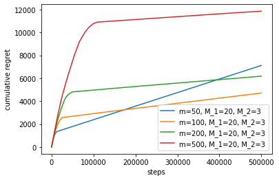
Figure 1: Cumulative regret for different $m$.

Once we fix $m$, we now examine the choices of $M_{1}$ and $M_{2}$. The parameters $M_{1}$ and $M_{2}$ determine the conditions of winning and losing: if counter gets to $M_{1}$, then the current arm beats the “virtual arm” and is therefore chosen as the best arm; if the counter gets to $-M_{2}$, then the current arm loses the tournament with the “virtual arm” and we move to a new arm. If all $K$ arms lose the tournament, we decrease the aspiration level by 1 and restart the tournament. We want it to be easier for the “virtual arm” to win, since the consequences are lower in that case (the protocol ends if we declare arm $i$ a winner, whereas we keep going if the “virtual arm” is a winner). Therefore, it makes sense to have an asymmetry and choose $M_{1}$ greater than $M_{2}$. We again consider an MAB $B$ with $K=50$ arms and $m=100$ fixed. As shown in Figure 2, the cumulative regret increases as $M_{1}$ and $M_{2}$ get larger. However, the gap between the success probability of the arm chosen by protocol $P$ and the success probability of the optimal arm of $B$, decreases. The corresponding gaps, averaged over 100 repetitions, are 0.014, 0.007, 0.005, 0.004, respectively. Since the number of states in the aspiration-level protocol is $Km(M_{1}+M_{2})$, there is a tradeoff between accuracy and the number of states required. Taking into account state-efficiency, accuracy, and the expected cumulative regret, we choose $M_{1}=20$ and $M_{2}=3$.

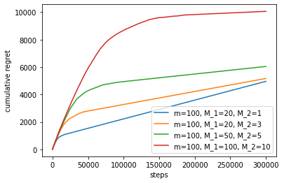
Figure 2: Cumulative regret for different $M_{1}$ and $M_{2}$.

Both Figure 1 and Figure 2 show that the performance of the aspiration-level protocol degrades quite gracefully as we take smaller values of $m$, $M_{1}$, and $M_{2}$ (which is how we would have to deal with having fewer states).

4.3 PARAMETER SETTINGS FOR THE ELIMINATION TOURNAMENT

The elimination-tournament protocol has two parameters: $M$ (the point at which an arm is declared a winner in the two-way comparison) and $N$ (recall that $1/N$ is the probability that an arm is declared in the two-way comparison if no arm is dominant and has $M$ more successes than the other). Thus, after an expected number of at most $N(K-1)$ steps, the elimination-tournament protocol has reduced to one arm. We clearly want $M$ and $N$ to be large enough to give the protocol time to select a relatively good arm. However, we don’t want to stick with bad arms for too long, since this will lead to larger cumulative regret. Figure 3 shows the cumulative regrets for different choices of $N$ and $M$, for an MAB with $K=50$ arms. For the choices of $(N,M)$ considered—(1000,10), (1000,20), (1000, 100), (100,10), (100,20)—the gaps, averaged 100 repetitions, are 0.01, 0.007, 0.006, 0.03, 0.03, respectively. Both $N=1000,M=20$ and $N=1000,M=100$ give similarly good performance in terms of the expected average regret, but the latter leads to larger expected cumulative regret. Therefore, for $K=50$, we choose $N=1000$ and $M=20$.

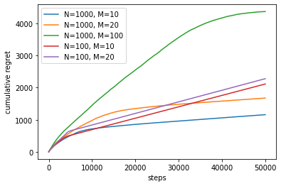
Figure 3: Cumulative regret for different $N$ and $M$.

4.4 COMPARING PROTOCOLS

Based on the simulations above, to minimize the number of states used while maintaining relatively good performance, for $K=50$, we choose the parameters $m=100,M_{1}=20,M_{2}=3$ for the aspiration-level protocol and $M=20$, $N=1000$ for the elimination-tournament protocol, and compare these two finite-state protocols to the $\epsilon$-greedy protocol and Thompson Sampling, which are infinite-state protocols. With these choices, the aspiration-level protocol uses 115,000 states, while the elimination-tournament protocol uses just over 100,000. While this may seem to be a a lot of states, they can be encoded using 17 bits. Given the number of neurons in a human brain, this should not be a problem.

We can greatly reduce the cumulative regret for the aspiration-level protocol by a preprocessing phase, as suggested earlier. For $K=50$ arms and the aspiration-level protocol with $m=100,M_{1}=20,M_{2}=3$, we first use a preprocessing phase to get a rough idea of what the true highest success probability might be. We use the parameters suggested earlier, decreasing the aspiration level by 10 after testing all the arms in the preprocessing, and use thresholds $M_{1}^{\prime}=-5$ and $M_{2}^{\prime}=-1$. We use this two-phase approach for the aspiration-level protocol in the following simulation.

We consider MABs with $K=50$ arms, and see how the elimination-tournament protocol, the aspiration-level protocol, $\epsilon$-greedy, and Thompson sampling perform. Not surprisingly, Thompson sampling performs best, and has logarithmic cumulative regret, whereas the other three protocols have linear cumulative regret. After 50,000 steps, the expected difference between the success probability of the arm chosen and that of the optimal arm for these protocols are 0.007, 0.008, 0.025, 0.003, respectively. Interestingly, both the aspiration-level protocol and the elimination-tournament protocol eventually outperform $\epsilon$-greedy, although the latter requires infinitely many states.

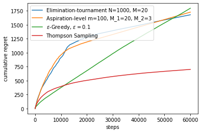
Figure 4: Cumulative regret over time.

5 DISCUSSION

We have introduced two finite-state protocols for playing MABs, the aspiration-level protocol and the elimination-tournament protocol. Both perform quite well in practice, while using relatively few states. In cases where switching between arms incurs a significant cost, the aspiration-level protocol is a better choice.

Recall that the main motivation for this study was understanding human behavior. The fact that the aspiration-level protocol exhibits such human-like behavior, including adjusting aspiration levels according to feedback, an optimism bias, a negativity bias, and a status quo bias, as well as a focus on recent behavior, suggests that humans are not being so irrational. Note that these biases are emphasized if the number of states is decreased. For example, if an agent decreases $M_{2}$, the threshold for rejecting an arm in a two-way comparison with the virtual arm, in response to having fewer states, this increases the negativity bias. Decreasing $M_{1}$ increases the likelihood that an agent will continue to play an apparently “lucky arm”. The impact of decreasing $M$ in the elimination-tournament protocol is similar. The bottom line is that these protocols exhibit apparently irrational behavior for quite rational reasons! At the same time, they may be of interest even for those not interested in modeling human behavior, since they have quite good performance, even with relatively few states.

We have focused here on a static setting, where the probabilities do not change over time. We could easily modify our PFA to deal with the dynamic setting by simply resetting the tournaments from time to time. More interestingly, we would like to apply these ideas to a more game-theoretic setting, such as the wildlife poaching setting considered by Kar et al. Kar15, where rangers are trying to protect rhinos from poachers. We hope to report on that in future work.

Acknowledgements

This research was supported by MURI (MultiUniversity Research Initiative) under grant W911NF-19-1-0217, by the ARO under grant W911NF-17-1-0592, by the NSF under grants IIS-1703846 and IIS-1718108, and by a grant from the Open Philosophy Foundation. We thank Alice Chen for her preliminary work and comments on an earlier version of the manuscript. We also thank four anonymous reviewers for their feedback.

References

- [\citeauthoryearErev, Ert, and RothErev et al.2010] Erev, I., E. Ert, and A. E. Roth (2010). A choice prediction competition for market entry games: An introduction. Games and Economic Behavior 1(1), 117–136.
- [\citeauthoryearGigerenzer and GaissmaierGigerenzer and Gaissmaier2015] Gigerenzer, G. and W. Gaissmaier (2015). Decision making: Nonrational theories. In J. D. Wright (Ed.), International Encyclopedia of the Social and Behavioral Sciences (2nd Edition), pp. 911–916.
- [\citeauthoryearHalpern, Pass, and SeemanHalpern et al.2012] Halpern, J. Y., R. Pass, and L. Seeman (2012). I’m doing as well as I can: modeling people as rational finite automata. In Proc. Twenty-Sixth National Conference on Artificial Intelligence (AAAI ’12), pp. 1917–1923.
- [\citeauthoryearKanouse and HansonKanouse and Hanson1972] Kanouse, D. E. and L. Hanson (1972). Negativity in evaluations. In E. E. Jones, D. E. Kanouse, S. Valins, H. H. Kelley, R. E. Nisbett, and B. Weiner (Eds.), Attribution: Perceiving the Causes of Behavior. Morristown, NJ: General Learning Press.
- [\citeauthoryearKar, Fang, Delle Fave, Sintov, and TambeKar et al.2015] Kar, D., F. Fang, F. Delle Fave, N. Sintov, and M. Tambe (2015). “Game of thrones”: when human behavior models compete in repeated Stackelberg security games. In Proc. 2015 International Conference on Autonomous Agents and Multiagent Systems, pp. 1381–1390.
- [\citeauthoryearKaufmann, Korda, and MunosKaufmann et al.2012] Kaufmann, E., N. Korda, and R. Munos (2012). Thompson sampling: an asymptotically optimal finite-time analysis. In N. H. Bshouty, G. Stoltz, N. Vayatis, and T. Zeugmann (Eds.), Algorithmic Learning Theory )ALT 2012), LNCS, Volume 7568, pp. 199–213. Springer.
- [\citeauthoryearLai and RobbinsLai and Robbins1985] Lai, T. L. and H. Robbins (1985). Asymptotically efficient adaptive allocation rules. Advances in Applied Mathematics 6(1), 4–22.
- [\citeauthoryearLewin, Dembo, Festinger, and SearsLewin et al.1944] Lewin, K., T. Dembo, L. Festinger, and P. S. Sears (1944). Level of aspiration. In J. M. Hunt (Ed.), Personality and the Behavior Disorders, pp. 333–378. Cambridge, MA: Ronald Press.
- [\citeauthoryearNeymanNeyman1985] Neyman, A. (1985). Bounded complexity justifies cooperation in finitely repeated prisoner’s dilemma. Economic Letters 19, 227–229.
- [\citeauthoryearPapadimitriou and YannakakisPapadimitriou and Yannakakis1994] Papadimitriou, C. H. and M. Yannakakis (1994). On complexity as bounded rationality. In Proc. 26th ACM Symposium on Theory of Computing, pp. 726–733.
- [\citeauthoryearRaoRao2017] Rao, A. (2017). A finite memory automaton for two-armed Bernoulli bandit problems. In Proc. Thirty-First National Conference on Artificial Intelligence (AAAI ’17), pp. 4981–4982. The full paper is available at http://raoariel.github.io/raoariel-fma.pdf.
- [\citeauthoryearRubinsteinRubinstein1986] Rubinstein, A. (1986). Finite automata play the repeated prisoner’s dilemma. Journal of Economic Theory 39, 83–96.
- [\citeauthoryearSamuelson and ZeckhauserSamuelson and Zeckhauser1998] Samuelson, W. and R. Zeckhauser (1998). Status quo bias in decision making. Journal of Risk and Uncertainty 1, 7–59.
- [\citeauthoryearSeltenSelten1998] Selten, R. (1998). Aspiration adaptation theory. Journal of Mathematical Psychology 42, 191–214.
- [\citeauthoryearSharotSharot2011] Sharot, T. (2011). The Optimism Bias: A Tour of the Irrationally Positive Brain. New York, NY: Pantheon Books.
- [\citeauthoryearSimonSimon1956] Simon, H. A. (1956). Rational choice and the structure of the environment. Psychological Review 63(2), 129–138.
- [\citeauthoryearSimonSimon1982] Simon, H. A. (1982). Models of bounded rationality. Cambridge, MA: MIT Press.
- [\citeauthoryearThalerThaler2015] Thaler, R. (2015). Misbehaving: The Making of Behavioral Economics. New York, NY: W. W. Norton and Company.
- [\citeauthoryearThompsonThompson1933] Thompson, W. R. (1933). On the likelihood that one unknown probability exceeds another in view of the evidence of two samples. Biometrika 25(3–4), 285–294.
- [\citeauthoryearTversky and KahnemanTversky and Kahneman1973] Tversky, A. and D. Kahneman (1973). Availability: a heuristic for judging frequency and probability. Cognitive Psychology 5, 207–232.
- [\citeauthoryearWilsonWilson2015] Wilson, A. (2015). Bounded memory and biases in information processing. Econometrica 82(6), 2257–2294.