Relation between Statics and Dynamics in the Quench of the Ising Model to below the Critical Point

Abstract

The standard phase-ordering process is obtained by quenching a system, like the Ising model, to below the critical point. This is usually done with periodic boundary conditions to insure ergodicity breaking in the low temperature phase. With this arrangement the infinite system is known to remain permanently out of equilibrium, i.e. there exists a well defined asymptotic state which is time-invariant but different from the ordered ferromagnetic state. In this paper we establish the critical nature of this invariant state, by demonstrating numerically that the quench dynamics with periodic and antiperiodic boundary conditions are indistinguishable one from the other. However while the asymptotic state does not coincide with the equilibrium state for the periodic case, it coincides instead with the equilibrium state of the antiperiodic case, which in fact is critical. The specific example of the Ising model is shown to be one instance of a more general phenomenon, since an analogous picture emerges in the spherical model, where boundary conditions are kept fixed to periodic, while the breaking or preserving of ergodicity is managed by imposing the spherical constraint either sharply or smoothly.

I Introduction

Macroscopic systems, in absence of an external drive, equilibrate with the environment. However, relaxation may be slow, i.e. with a relaxation time which exceeds any attainable observation time Palmer . In that case, only dynamical properties are accessible to observation and the question naturally arises of what can be learnt about equilibrium from dynamics. Paradigmatical examples of slow relaxation are glassy systems BCKM or systems undergoing phase ordering after a sudden temperature quench from above to below the critical point BCKM ; Bray . Here we shall look at the problem in the latter context, whose prototypical instance is the quench of a ferromagnetic system. In order to make the presentation as simple as possible, we shall mostly concentrate on the Ising model. The extension to other phase-ordering systems will be discussed at the end of the paper, with the example of the spherical model.

Phase ordering in the Ising model by now is a mature subject, generally considered to be well understood. For reviews see Refs. Bray ; Puri ; Jo ; Henkel . Among the many interesting features of the process, in this paper we shall be primarily concerned with the lack of equilibration in any finite time, if the system is infinite. This is frequently referred to with the catchy expression that the system remains permanently out of equilibrium, whose meaning, however, has never been fully clarified. For instance, a similar circumstance arises also when the quench is made to the critical temperature $T_{c}$, because, due to critical slowing down, again equilibrium is not reached in any finite time. Nonetheless, in that case, the process cannot be regarded as substantially different from one of equilibration, because as time grows the system gets closer and closer to the equilibrium critical state, which is unique in the sense that in the thermodynamic limit it is independent of the boundary conditions (BC). Instead, in the quench to below $T_{c}$ the picture is qualitatively different, because, although the state extrapolated from dynamics is unique, the same cannot be said of the equilibrium state, which depends on BC even in the thermodynamic limit. This we have shown in Ref. FCZ (to be referred to as I in the following), where we have investigated the nature of the equilibrium state in the Ising model below $T_{c}$, under different symmetry-preserving BC. We have found that while periodic boundary conditions (PBC) lead to the usual ferromagnetic ordering, due to the breaking of ergodicity with the consequential spontaneous breaking of the $\mathbb{Z}_{2}$ up-down symmetry, the scenario changes dramatically with antiperiodic boundary conditions (APBC), because ergodicity breaking is precluded. Then, the system cannot order and complies with the requirement of the transition by remaining critical also below $T_{c}$, all the way down to $T=0$. We have argued that this new transition, without spontaneous symmetry breaking and without ordering, consists in the condensation of fluctuations. In the $1d$ case, since $T_{c}=0$, the low temperature phase is shrunk to just $T=0$.

Motivated by the existence of such diversity in the equilibrium properties, in this paper we address the next natural question, formulated in the title of the paper, of matching statics and dynamics. Using the equal-time correlation function as the probing observable, we shall see that the asymptotic state, extrapolated from dynamics, that is by taking the $t\to\infty$ limit after the thermodynamic limit, is unique and critical. Now, the point is that this, which we may call the time-asymptotic state and which, we emphasize, is the same for both choices of BC, is found to coincide with the bona fide equilibrium state, i.e. the one computed from equilibrium statistical mechanics, in the APBC case but to be remote from it in the PBC case. Thus, we have the one and the same dynamical evolution which, although not reaching equilibrium in any finite time, turns out to be informative of the true equilibrium state in one case (APBC), but not in the other (PBC). It is, then, appropriate to regard the APBC case as one in which equilibrium is approached, just as in a quench to $T_{c}$, while the PBC case offers an instance of a system remaining permanently out of equilibrium. The poor performance in approaching equilibrium with PBC is traceable to the presence of ergodicity breaking at the working temperature, which, instead, is preserved when APBC are applied. At the end of the paper we shall argue that the connection between the presence/absence of ergodicity breaking and the absence/presence of equilibration goes beyond the Ising example, by showing that it takes place with the same features in the rather different context of the spherical and mean-spherical model.

The paper is organized as follows: in section II we formulate the problem. In section III the relation between equilibrium and relaxation in the quench to above $T_{c}$ is analyzed by using scaling arguments. The cases of the quench to $T_{c}$ with $d=2$, to $T=0$ with $d=1$ and to below $T_{c}$ with $d=2$ are analyzed in sections IV, V and VI, respectively. The spherical and mean spherical model are introduced and investigated in section VII. Concluding remarks are made in section VIII.

II The problem

We are concerned with the relaxation dynamics of a system initially prepared in an equilibrium state at the temperature $T_{I}$ and suddenly quenched to the lower temperature $T_{F}$. We consider the Ising model on a lattice of size $V=L^{d}$, with the usual nearest neighbours interaction

$${\cal H}(\boldsymbol{s})=-J\sum_{<ij>}s_{i}s_{j},$$ (1)

where $J>0$ is the ferromagnetic coupling, $\boldsymbol{s}=[s_{i}]$ is a configuration of spin variables $s_{i}=\pm 1$ and $<ij>$ is a pair of nearest neighbours. We shall study the $d=1$ and $d=2$ cases, where in the thermodynamic limit there is a critical point at $T_{c}=0$ and $T_{c}=2.269J$, respectively. Since the system’s size is finite, BC must be specified and, because of the major role that these will play in the following developments, it is necessary to enter in some detail from the outset. As anticipated in the Introduction, we shall consider PBC and APBC (precisely cylindrical antiperiodic BC) implemented by adding to the interaction an extra term ${\cal B}(\boldsymbol{s})$ with couplings among spins on the boundary Gallavotti ; Antal ; FCZ . In the $d=2$ case spins on opposite edges are coupled ferromagnetically, just like spins in the bulk, if PBC are applied. Instead, in the APBC case, spins on one pair of opposite edges are coupled ferromagnetically, while those on the other pair antiferromagnetically. Hence, the boundary term reads

$${\cal H}_{b}(\boldsymbol{s})=-J\sum_{y=1}^{L}s_{1,y}s_{L,y}-bJ\sum_{x=1}^{L}s_{x,1}s_{x,L},$$ (2)

where we have denoted by $b=\pm$ the sign of $J$, which identifies PBC $(+)$ or APBC $(-)$. In the $d=1$ case this term simplifies to

$${\cal H}_{b}(\boldsymbol{s})=-bJs_{1}s_{L},$$ (3)

where $L$ is the length of the chain. It is important to note that both these BC preserve the up-down symmetry of the Ising interaction.

Taking as it is customary $T_{I}=\infty$ in order to have an uncorrelated initial state, the system is put in contact with a thermal reservoir at the lower and finite temperature $T_{F}$ and let to evolve according to a dynamical rule which does not conserve the order parameter, like Glauber or Metropolis. This simply corresponds to running a Markov chain at the fixed temperature $T_{F}$, with the so-called hot start, that is with a uniformly random initial condition. The relaxation process is monitored through the equal-time spin-spin correlation function

$$\mathcal{C}(r,\epsilon,t^{-1},L^{-1};b)=\left[\langle s_{i}(t)s_{j}(t)\rangle-\langle s_{i}(t)\rangle\langle s_{j}(t)\rangle\right],$$ (4)

where the angular brackets denote averages taken over the noisy dynamics and the initial conditions, while the square brackets stand for the average over all pairs of sites $(i,j)$ keeping fixed the distance $r$ between $i$ and $j$. In the set of control parameters, $\epsilon=T_{F}-T_{c}$ is the temperature difference from criticality, $t^{-1}$ is the inverse time and $L^{-1}$ is the inverse linear size.

We are interested in taking both the large-time and the thermodynamic limit of the above quantity, and then to compare the outcomes, depending on the order in which these two limits have been taken. Letting $t^{-1}\to 0$ first, while keeping $L$ fixed, the equilibrium correlation function is obtained

$$\lim_{t^{-1}\to 0}\mathcal{C}(r,\epsilon,t^{-1},L^{-1};b)=\mathcal{C}_{\rm eq}(r,\epsilon,L^{-1};b)=\left[\langle s_{i}s_{j}\rangle_{\rm eq}-\langle s_{i}\rangle_{\rm eq}\langle s_{j}\rangle_{\rm eq}\right],$$ (5)

where now the angular brackets stand for the Gibbs ensemble average and the square brackets have the same meaning as in Eq. (4). Then, the subsequent thermodynamic limit implements the prescription Gallavotti for the construction of the equilibrium correlation function in the infinite system

$$\lim_{L^{-1}\to 0}\lim_{t^{-1}\to 0}\mathcal{C}(r,\epsilon,t^{-1},L^{-1};b)=C_{\rm eq}(r,\epsilon;b).$$ (6)

The crux of the matter is that, after reversing the order of these limits, the end result might not be the same as the one above, because the large-time limit of the time-dependent correlation function for the infinite system

$$\lim_{t^{-1}\to 0}\lim_{L^{-1}\to 0}\mathcal{C}(r,\epsilon,t^{-1},L^{-1};b)=C^{*}(r,\epsilon;b),$$ (7)

exists but does not necessarily coincide with $C_{\rm eq}(r,\epsilon;b)$. Referring to $C^{*}(r,\epsilon;b)$ as the time-asymptotic correlation function, if it matches $C_{\rm eq}(r,\epsilon;b)$ then the infinite system equilibrates. If not, it remains permanently out of equilibrium. Which is the case depends on $T_{F}$ and on the choice of BC. In the quench to $T_{F}\geq T_{c}$ both $C_{\rm eq}(r,\epsilon)$ and $C^{*}(r,\epsilon)$ are independent of the BC choice and do coincide, signaling equilibration. Instead, in the quench to below $T_{c}$, as we shall see, $C^{*}(r,\epsilon)$ does not depend on $b$, while $C_{\rm eq}(r,\epsilon;b)$ retains this dependence, implying that equilibration can be achieved at most with one of the two BC, but certainly not with both. As anticipated in the Introduction, the equilibration condition is fulfilled with APBC, but not with PBC.

In the next section we shall substantiate the above statements with results for the $1d$ and $2d$ Ising model. We shall take the aforementioned limits, after setting up the general scaling scheme which unifies static and dynamic phenomena into one single framework encompassing both. In order to do this, it is convenient to treat separately the three cases: $\epsilon>0$, $\epsilon=0$ and $\epsilon<0$.

III Statics and Dynamics: $\boldsymbol{\epsilon>0}$

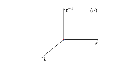
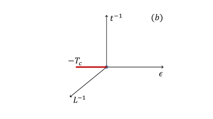
Figure 1: Parameter space of the $1d$ model (a) and of the $2d$ model (b).

Let us assume that at a generic point in the $\epsilon>0$ sector of the three-dimensional space of the parameters $(\epsilon,t^{-1},L^{-1})$, depicted in Fig.1, the correlation function obeys scaling in the form 

$$\mathcal{C}(r,\epsilon,t^{-1},L^{-1};b)=\frac{1}{r^{a}}\mathcal{F}\left(\frac{r}{\ell},\frac{\ell}{R},\frac{R}{L};b\right),$$ (8)

where the exponent $a$ is related to the anomalous dimension exponent $\eta$ by $a=d-2+\eta$ and to the fractal dimensionality $D$ of the Coniglio-Klein (CK) CK ; FK correlated clusters CF by

$$a=2(d-D).$$ (9)

From the exact results Stanley ; Goldenfeld

$$\eta=\left\{\begin{array}[]{ll}1,\;\;$for$\;\;d=1,\\ 1/4,\;\;$for$\;\;d=2,\end{array}\right.$$ (10)

follows

$$a=\left\{\begin{array}[]{ll}0,\;\;$for$\;\;d=1,\\ 1/4,\;\;$for$\;\;d=2,\end{array}\right.$$ (11)

and

$$D=\left\{\begin{array}[]{ll}1,\;\;$for$\;\;d=1,\\ 15/8,\;\;$for$\;\;d=2,\end{array}\right.$$ (12)

which shows that the CK clusters are compact in $1d$ and fractals in $2d$. Up to a proportionality constant, the scaling variable $\ell$ is the equilibrium correlation length of the infinite system, given by Stanley

$$\ell(\epsilon)=\left\{\begin{array}[]{ll}-[\ln\tanh(J/\epsilon)]^{-1},\;\;$for$\;\;d=1,\\ \epsilon^{-\nu},\;\;$with$\;\;\nu=1\;\;$for$\;\;d=2.\end{array}\right.$$ (13)

The other characteristic length $R(t)$ obeys the power law Janssen

$$R(t)=t^{1/z},$$ (14)

with the dynamical exponent 1d ; Nightingale

$$z=\left\{\begin{array}[]{ll}2,\;\;$for$\;\;d=1,\\ 2.16,\;\;$for$\;\;d=2.\end{array}\right.$$ (15)

The connection between $R(t)$ and the time dependent correlation length will be clarified shortly and is summarized in Fig.2. Both lengths diverge as the critical point, which is at the origin of the reference frame in Fig.1, is approached along the $\epsilon$ axis and the $t^{-1}$ axis, respectively.

The scaling ansatz (8) is dense of information and allows to predict what should be expected in different regions of the parameter space. The foremost relevant features are the power-law decay $1/r^{a}$ of correlations at short distance and the large-distance cutoff enforced by the scaling function. The separation between short and large distances is fixed by the correlation length

$$\xi(\epsilon,t^{-1},L^{-1};b)=\left[\frac{\int_{0}^{L}dr\,r^{2}\,\mathcal{C}(r,\epsilon,t^{-1},L^{-1};b)}{\int_{0}^{L}dr\,\mathcal{C}(r,\epsilon,t^{-1},L^{-1};b)}\right]^{1/2},$$ (16)

which scales as

$$\xi(\epsilon,t^{-1},L^{-1};b)=Rf\left(\frac{R}{\ell},\frac{\ell}{L};b\right).$$ (17)

The behaviour of $\xi$, as parameters are changed, can be unraveled by the following argument. Suppose that $\ell$ and $L$ are fixed in a region where $\ell\ll L$ and let us survey what happens as the quench unfolds and $R$ grows.

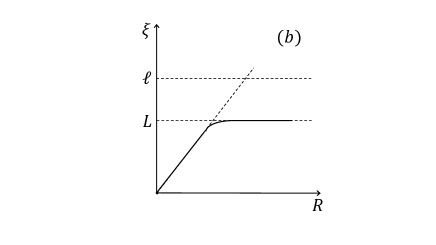
Figure 2: Schematic representation of the saturation of $\xi$ vs $R$ for $\ell\ll L$ (a) and for $\ell\gg L$ (b).

Approximating the above equation by

$$\xi(\epsilon,t^{-1})\simeq Rf\left(\frac{R}{\ell},0\right),$$ (18)

in the early stage of the quench, when $R\ll\ell$, it can be further reduced to

$$\xi\sim R,$$ (19)

because the system behaves as if it was approaching the critical point along the $t^{-1}$ axis. As $R$ is let to grow further, equilibrium is eventually reached when $R\sim\ell$ and the correlation length saturates to the limiting value

$$\xi\sim\ell,$$ (20)

as illustrated in the left panel of Fig.2, with the equilibration time given by $t_{\rm eq}=\ell^{z}$. The BC are immaterial throughout, because $\xi$ remains always much smaller than $L$ so that the system as a whole behaves as a collection of independent finite systems, on which the far away BC have no effect. By the same reasoning, in the region where $\ell\gg L$ we still have $\xi\sim R$ in the early stage, when $R\ll L$, with independence from BC. But then BC come into play when the system equilibrates and $\xi$ saturates to the limiting value $L$, as illustrated in the right panel of Fig.2, since correlations extend up to distances where the BC are effective. In this connection see Ref. Das . Summarizing, $\xi$ is given by the shortest of the three lengths $(\ell,R,L)$, that is

$$\xi(\epsilon,t^{-1},L^{-1})\sim\min(\ell,R,L),$$ (21)

in the regions of the parameter space where one of the three is considerably shorter than the other two, with crossovers connecting these regions. It is clear from Fig.2 that $\xi$ and $R$ coincide at all times if both $\ell$ and $L$ are infinite. Next to the correlation length, it is useful to keep track also of the susceptibility

$$\chi(\epsilon,t^{-1},L^{-1};b)=\int d^{d}r\,\mathcal{C}(r,\epsilon,t^{-1},L^{-1};b),$$ (22)

which is related to the correlation length by

$$\chi\sim\xi^{2D-d}.$$ (23)

This is an important relation, because it is independent of the direction of approach to the critical point and depends only on the geometrical nature of the correlated clusters through $D$.

According to the above reasoning, when the limits $t^{-1}\to 0$ and $L^{-1}\to 0$ are taken in the $\epsilon>0$ sector, we necessarily have $\xi\sim\ell$, independently of the order in which these limits are taken, because $\ell$ is finite. Moreover, the finite correlation length guarantees that the system equilibrates with independence from BC

$$\lim_{L^{-1}\to 0}\lim_{t^{-1}\to 0}\mathcal{F}\left(\frac{r}{\ell},\frac{\ell}{R},\frac{R}{L};b\right)=\lim_{t^{-1}\to 0}\lim_{L^{-1}\to 0}\mathcal{F}\left(\frac{r}{\ell},\frac{\ell}{R},\frac{R}{L};b\right)=F_{\rm eq}\left(\frac{r}{\ell}\right).$$ (24)

III.1 Example: $1d$ system

As an example, let us check the above statements against exact results in the particular case of the $t^{-1}\to 0$ limit of the $1d$ model with finite $L$. The equilibrium correlation function is given by

$$\mathcal{C}_{\rm eq}(r,\epsilon,L^{-1};b)=\frac{1}{r^{a}}\mathcal{F}_{\rm eq}\left(\frac{r}{L},\frac{L}{\ell};b\right),$$ (25)

where $a=0$ according to Eq. (15), while the two explicit forms of the scaling function (see I and Ref. Antal ) read

$$\mathcal{F}^{(p)}_{\rm eq}(z,\zeta)=\frac{\cosh[\zeta(1-z)]}{\cosh(\zeta)},$$ (26)

$$\mathcal{F}^{(a)}_{\rm eq}(z,\zeta)=\frac{\sinh[\zeta(1-z)]}{\sinh(\zeta)},$$ (27)

where we have set

$$z=r/L,\quad\zeta=L/\ell.$$ (28)

We have considered a chain of length $2L$ in order to simplify notation. The superscripts $(p)$ and $(a)$ have been used for PBC and for APBC, respectively. The equilibrium correlation length, defined through the second moment as in Eq. (16), scales as

$$\xi_{\rm eq}(\epsilon,L^{-1};b)=\ell f_{\rm eq}(\zeta;b),$$ (29)

with the scaling functions

$$f_{\rm eq}^{(p)}(\zeta)=\left[2-\frac{2\zeta}{\sinh(\zeta)}\right]^{1/2},\quad f_{\rm eq}^{(a)}(\zeta)=\left[2-\frac{\zeta^{2}}{\cosh(\zeta)-1}\right]^{1/2},$$ (30)

from which follows

$$\xi_{\rm eq}^{(p)}(\epsilon,L^{-1})=\left\{\begin{array}[]{ll}\sqrt{2}\,\ell,\;\;$for$,\;\;\ell\ll L,\\ \frac{1}{\sqrt{3}}\,L,\;\;$for$,\;\;L\ll\ell,\end{array}\right.\quad\xi_{\rm eq}^{(a)}(\epsilon,L^{-1})=\left\{\begin{array}[]{ll}\sqrt{2}\,\ell,\;\;$for$,\;\;\ell\ll L,\\ \frac{1}{\sqrt{6}}\,L,\;\;$for$,\;\;L\ll\ell,\end{array}\right.$$ (31)

showing that in the regimes $\ell\ll\L$ and $\ell\gg L$, indeed one has $\xi\sim\min(\ell,L)$. Completing, next, the sequence of limits by letting $L^{-1}\to 0$, it is straightforward to check that the dependence on BC disappears, yielding

$$\lim_{L^{-1}\to 0}\mathcal{F}^{(p)}_{\rm eq}(z,\zeta)=\lim_{L^{-1}\to 0}\mathcal{F}^{(a)}_{\rm eq}(z,\zeta)=e^{-r/\ell}.$$ (32)

Using the definition, it is immediate to verify that also $\chi\sim\ell$ and, therefore, that moving toward the critical point along the $\epsilon$ axis one has

$$\chi\sim\xi,$$ (33)

in agreement with Eq. (23), because $D=1$ when $d=1$.

IV Statics and Dynamics: $\boldsymbol{\epsilon=0,d=2}$

When $\epsilon=0$, the $1d$ and $2d$ cases are quite different and need to be treated separately. In the latter one, which we shall now consider, $T_{c}>0$ and ergodicity does not break. In the former, instead, $T_{c}=0$ and ergodicity may break, depending on BC. This makes it more akin to the $2d$ quench to below $T_{c}$. So, it will be dealt with in the next section.

Figure 3: Scaling function of the time-dependent correlation function in the quench to $T_{c}$ of the $2d$ model, demonstrating independence from BC, in the system with $L=256$. PBC (black symbols) and APBC (empty symbols).

The specificity of the quench to $\epsilon=0$ is that $\ell$ diverges and, consequently, that $\xi$ can be limited only by $R$ or $L$. Thus, when the $t^{-1}\to 0$ limit is taken first and $L$ is kept fixed, $\xi$ crosses over from $R$ to $L$ in the finite time $t_{\rm eq}\sim L^{z}$, as in the right panel of Fig.2, and the system equilibrates to

$$\mathcal{C}_{\rm eq}(r,L^{-1};b)=\frac{1}{r^{1/4}}\mathcal{F}_{\rm eq}\left(\frac{r}{L};b\right),$$ (34)

which depends on BC because correlations extend up to the boundary. Letting next $L^{-1}\to 0$, the BC dependence disappears from the critical correlation function of the infinite system

$$C_{\rm eq}(r)\sim\frac{1}{r^{1/4}}.$$ (35)

Instead, if the $L^{-1}\to 0$ limit is taken first, $R$ is the only length left in the problem. This implies $\xi\sim R$ at all times, so that there is no finite equilibration time. However, the time-dependent correlation function

$$C(r,t^{-1})=\frac{1}{r^{1/4}}F_{c}(r/R),$$ (36)

which is BC independent (see Fig.3), gets arbitrarily close to the equilibrium counterpart (35) as time grows, because the limit

$$\lim_{t^{-1}\to 0}C(r,t^{-1})=C^{*}(r)\sim\frac{1}{r^{1/4}},$$ (37)

coincides with it. In summary, in the quench to $\epsilon=0$ of the $2d$ system, like in the $\epsilon>0$ case previously considered, the equilibrium correlation function of the infinite system $C_{\rm eq}(r)$ does not depend on BC and coincides with the time-asymptotic one $C^{*}(r)$, warranting the conclusion that the system can get arbitrarily close to equilibrium by waiting long enough.

Comparing Eqs. (34) and (36), it is evident that the scaling structure is the same, the only difference being in the specific forms of the scaling functions, which is inessential for the present considerations. This shows that the time direction along the $t^{-1}$ axis, as far as scaling is concerned, is just another direction of approach to the critical point, on the same footing with the other two. In addition, from the formal similarity of the two scaling expressions follows straightforwardly that the susceptibility satisfies Eq. (23) in the form

$$\chi\sim\xi^{7/4},$$ (38)

irrespective of the direction of approach, with $\xi\sim L$ along the $L^{-1}$ axis and $\xi\sim R$ along the $t^{-1}$ axis.

V Statics and Dynamics: $\boldsymbol{\epsilon=0,d=1}$

As mentioned above and explained at length in I, in the $1d$ system at $\epsilon=0$ we are confronted with a radically different situation, because ergodicity, which holds for both BC above $T_{c}$, is now broken with PBC, but not with APBC. In order to ease the comparison, and to highlight the contrast, with the less familiar case of a transition without ergodicity breaking, let us first briefly summarize the well-established concept of ergodicity breaking Palmer . In the PBC case there are two degenerate ground states: the two ordered configurations with all spins either up $\boldsymbol{s}_{+}=[s_{i}=+1]$ or down $\boldsymbol{s}_{-}=[s_{i}=-1]$. These, by themselves, form two absolutely-confining ergodic components, which are dynamically disconnected because the activated moves needed to go from one to the other are forbidden at zero temperature. Consequently, time averages coincide with ensemble averages taken with either one of the two broken-symmetry ferromagnetic pure states $P_{-}(\boldsymbol{s})=\delta_{\boldsymbol{s},\boldsymbol{s}_{-}},P_{+}(\boldsymbol{s})=\delta_{\boldsymbol{s},\boldsymbol{s}_{+}}$ and do not coincide with the symmetric ensemble averages taken in the Gibbs state, which is the even mixture of the pure states

$$P^{(p)}(\boldsymbol{s})=\frac{1}{2}[P_{-}(\boldsymbol{s})+P_{+}(\boldsymbol{s})].$$ (39)

In such a situation, only time averages are physically meaningful. Conversely, in the APBC case all the $4L$ degenerate ground-state configurations with one defect (or domain wall) belong to the same ergodic component, because the defect can freely sweep the whole system at no energy cost. Then, in this case time and ensemble averages coincide. The qualitative difference between the two zero-temperature states is well illustrated (see Fig.4) by the probability distribution $P_{b}(m)$ of the magnetization density $m=\frac{1}{2L}\sum_{i}s_{i}$, which is demonstrated Antal to be double peaked in the PBC case

$$P^{(p)}(m)=\frac{1}{2}[\delta(m+1)+\delta(m-1)],$$ (40)

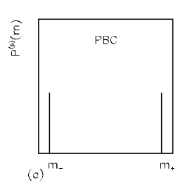
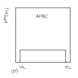
Figure 4: Magnetization density distributions at $\epsilon=0$ in the $1d$ Ising model, with $m_{\pm}=\pm 1$. The spikes in the panel (a) stand for $\delta$ functions.

and uniform over the $[-1,1]$ interval in the APBC case

$$P^{(a)}(m)\to\left\{\begin{array}[]{ll}1/2,\;\;$for$,\;\;m\in[-1,1],\\ 0,\;\;$for$,\;\;m\notin[-1,1].\end{array}\right.$$ (41)

So, if we now take the $t^{-1}\to 0$ limit while keeping $L^{-1}$ fixed, we find BC-related differences in the results. With PBC, as explained above, the meaningful averages are those in the broken symmetry pure states, yielding

$$\mathcal{C}^{(p)}_{\rm eq}(r,L^{-1})=[\langle s_{i}s_{j}\rangle_{\pm}-\langle s_{i}\rangle_{\pm}\langle s_{j}\rangle_{\pm}]=0,$$ (42)

where the angular brackets stand for the average with respect to $P_{-}(\boldsymbol{s})$ or $P_{+}(\boldsymbol{s})$. The vanishing of correlations for any $r$ holds independently of $L$ and clearly implies that also the correlation length vanishes. Notice that if the correlation function had been extracted by taking the $\epsilon\to 0$ limit of the Gibbs average taken with the distribution (39), as in Eq. (26), the result would have been

$$\mathcal{C}^{(p)}_{\rm eq}(r,L^{-1})=1,$$ (43)

which is independent of $r$ and does not decay. However, this would have been just an artefact of the mixture.

Conversely, in the APBC case the ensemble Gibbs average, as calculated in Eq. (27), gives the correct time-average result because ergodicity is not broken. Hence, in the $\epsilon\to 0$ limit, from Eq. (27) one has

$$\mathcal{C}^{(a)}_{\rm eq}(r,L^{-1})=(1-r/L).$$ (44)

The dependence on $r/L$ in the above expression reveals that correlations extend over a distance of order L in agreement with the general argument expounded in section III. Hence, by letting $L^{-1}\to 0$ the correlation length diverges, leading to the conclusion that the state at the origin of the parameter space is a critical point for the APBC system, where the correlation function displays the constant behaviour

$$C^{(a)}_{\rm eq}(r)=1.$$ (45)

Contrary to Eq. (43), now the lack of decay is a real physical effect, which corresponds to the critical power law decay $1/r^{a}$ with a vanishing exponent $a$, due to the compactness of the CK correlated clusters.

When the sequence of limits is reversed, after taking the thermodynamic limit we are again in the situation in which $R$ is the only length in the problem. Therefore $\xi\sim R$, as in the previous section, and we get the BC independent result

$$C(r,t^{-1})=\frac{1}{r^{a}}F(r/R),$$ (46)

with $a=0$. The function $F(x)$ is known from exact analytical computation with PBC 1d ; Bray and is given by

$$F(x)=\mathrm{erfc}\,(x),\quad\text{with}\quad x=r/2R.$$ (47)

That the same scaling function applies also to the case of APBC is demonstrated by the numerical data displayed in Fig. 5, which have been obtained by simulating the quench dynamics with the Metropolis algorithm on a system with $L=10^{5}$, after imposing PBC and APBC. The plot shows that the above result indeed holds irrespective of the BC choice, because the PBC and APBC data superimpose to the theoretical curve of Eq. (47) with great accuracy, as long as $R(t)\ll L$. The existence of an endlessly growing correlation length $R(t)$ means that the relaxation dynamics along the $t^{-1}$axis drives both systems, with PBC and with APBC, toward the same asymptotic critical state at the origin

Figure 5: Collapse on the master curve of Eq. (47) of the data for $C(r,t^{-1},L^{-1})$ in the time regime $R\ll L$. PBC (black symbols) and APBC (empty symbols). The data for $R/L=10^{-4},10^{-3}$ have been obtained with $L=10^{5}$, those with $R/L=10^{-2}$ with $L=10^{4}$.

with the unique time-asymptotic correlation function given by

$$\lim_{t^{-1}\to 0}C(r,t^{-1})=C^{*}(r)=1,$$ (48)

which coincides with the APBC equilibrium result in Eq.(45). So, if we compare the asymptotic result of Eq. (48) with the APBC static one of Eq. (45), and with the PBC equilibrium result of Eq. (42), we see, as stated in the Introduction, that the APBC system tends toward equilibrium, although with an infinite relaxation time, while the PBC system remains permanently out of equilibrium. It is evident that the origin of the diversity of behaviours is in the presence or absence of ergodicity breaking. In fact, we shall see in the next section that the same behaviour occurs in the quench of the $2d$ system to below the critical point.

In order to complete the picture of critical behaviour, let us check on the validity of Eq. (23). From Eqs. (32,44,47) follows that along the three directions one has $\xi\sim\ell,\xi\sim R,\xi\sim L$, as well as $\chi\sim\ell,\chi\sim R,\chi\sim L$, yielding

$$\chi\sim\xi,$$ (49)

independently of the direction of approach to the critical point, as it should be since $D=1$.

VI Statics and Dynamics: $\boldsymbol{\epsilon<0,2d}$

As in the previous case, the nature of the equilibrium state of the $2d$ model below $T_{c}$ depends strongly on BC, even in the thermodynamic limit. In I we have shown that the segment with $\epsilon<0$ in the parameter space (see right panel of Fig.1) is the coexistence line of states spontaneously-magnetized in opposite directions, when PBC are imposed, while it is a line of critical points with APBC. Since this is a crucial point, let us overview the equilibrium picture before turning to the discussion of the quench dynamics.

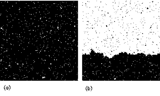
Figure 6: Typical equilibrium configurations below $T_{c}$. In the PBC case (a) one black domain of up spins fills the entire systems. Thermal fluctuations produce the small white domains of down spins. In the APBC case (b) there are two large domains separated by one interface cutting across the system. Within each domain there are the small patches of reversed spins due to thermal fluctuations.

VI.1 Equilibrium with PBC

When PBC are imposed, two confining components of spins aligned either prevalently up or prevalently down, are formed in phase space. A configuration typical of the up component is shown in the left panel of Fig.6. In the thermodynamic limit these components become absolutely confining, ergodicity breaks down and, therefore, we are confronted with the same situation discussed in the $1d$ case at $T=0$. Namely, the Gibbs state becomes the even mixture of the two broken-symmetry pure states like in Eq. (39), that is

$$P_{\rm eq}^{(p)}(\boldsymbol{s})=\sum_{\alpha}p(\alpha)P_{\alpha}(\boldsymbol{s}).$$ (50)

Here, $\alpha=\pm$ is the component label, the mixing probability is uniform $p(\alpha)=1/2$ and $P_{\alpha}(\boldsymbol{s})$ is the ferromagnetic pure state. The nonvanishing spontaneous magnetization density $m_{\alpha}$ is given by

$$m_{-}=-m_{+},\quad|m_{\alpha}|=|\epsilon|^{\beta},\quad\beta=1/8.$$ (51)

Using the above definitions and rewriting the Gibbs average in terms of the component averages, i.e. $\langle\cdot\rangle_{\rm eq}=\sum_{\alpha}p(\alpha)\langle\cdot\rangle_{\alpha}$, the equilibrium correlation function can be rearranged in the form

$$C_{\rm eq}^{(p)}(r,\epsilon)=\overline{\langle(s_{i}-m_{\alpha})(s_{i+r}-m_{\alpha})\rangle_{\alpha}}\;+\;\overline{[\langle s_{i}\rangle_{\alpha}-\overline{m_{\alpha}}][\langle s_{i+r}\rangle_{\alpha}-\overline{m_{\alpha}}]},$$ (52)

where the overline denotes averaging with respect to $p(\alpha)$. The first contribution is the average over components of the intra-component correlation function $\langle\psi_{i}\psi_{i+r}\rangle_{\alpha}$, where the variables $\psi_{i}=s_{i}-m_{\alpha}$ represent the thermal fluctuations in the pure state $P_{\alpha}(\boldsymbol{s})$. As it is intuitively clear, deviations from the average by symmetry do not depend on $\alpha$, so we shall use the notation $G_{\rm eq}(r,\epsilon)$ for $\langle\psi_{i}\psi_{i+r}\rangle_{\alpha}$. At low $T_{F}$ this quantity is short ranged, since in the broken-symmetry state the correlation length $\xi_{\psi}$ of the $\psi$ variables vanishes as $T_{F}\to 0$. The second term, instead, represents the inter-components contribution, which reduces to $m^{2}_{\alpha}$, since $\overline{m_{\alpha}}=0$ and $m^{2}_{\alpha}$ is independent of $\alpha$. Thus, in the end, from the Gibbs average we have

$$C_{\rm eq}^{(p)}(r,\epsilon)=G_{\rm eq}(r,\epsilon)+m^{2}_{\alpha}.$$ (53)

It is important, for what follows, to keep in mind that the constant term $m^{2}_{\alpha}$, which is the variance of the variable $m_{\alpha}$ distributed according to $p(\alpha)$, arises exclusively from the mixing as the constant term in Eq. (43). Therefore, in the PBC case the only dynamical variables are the $\psi_{i}$, which means that the dynamical rule updates $\psi_{i}$, but not $m_{\alpha}$. The magnetization distribution exhibits the double peak structure Binder ; Bruce which, in the thermodynamic limit, becomes the sum of the two $\delta$ functions

$$P^{(p)}(m|\epsilon)=\frac{1}{2}[\delta(m-m_{-})+\delta(m-m_{+})].$$ (54)

Hence, as explained in the $1d$ case, the meaningful averages are those taken with the broken symmetry ensembles $P_{\alpha}(\boldsymbol{s})$, which coincide with time averages and give

$$C_{\alpha,\rm eq}^{(p)}(r,\epsilon)=G_{\rm eq}(r,\epsilon).$$ (55)

VI.2 Equilibrium with APBC

When APBC are imposed, like in the $1d$ case ergodicity does not break. As explained in I, there is only one ergodic component, whose typical configurations at sufficiently low $T_{F}$ are composed of two large ordered domains, separated by one interface cutting across the system and sweeping through it, as illustrated in the right panel of Fig.6. This suggests to split the spin variable into the sum of two independent components

$$s_{i}=m_{\alpha(i)}+\psi_{i},$$ (56)

where $\alpha(i)=\pm$ is the label of the domain to which the site $i$ belongs and $\psi_{i}=s_{i}-m_{\alpha(i)}$ is, as before, the thermal fluctuation variable. The significant difference with respect to the previous case is that now $\psi_{i}$ and $m_{\alpha(i)}$ are both dynamical variables, since the fluctuations of the latter one are not due to the mixing of pure states, but to the transit of the interface through the site $i$, which means that the dynamical rule updates both $\psi_{i}$ and $m_{\alpha(i)}$. Using the independence of these variables and the vanishing of averages $\langle s_{i}\rangle_{\rm eq}=\langle m_{\alpha(i)}\rangle_{\rm eq}=\langle\psi_{i}\rangle_{\rm eq}=0$, the correlation function can be written as the sum of two contributions

$$C_{\rm eq}^{(a)}(r,\epsilon,L^{-1})=G_{\rm eq}(r,\epsilon)+D_{\rm eq}(r,\epsilon,L^{-1}),$$ (57)

which have quite different properties. The first one, which is the same as in Eq. (53), is short ranged. The $L$ dependence has been neglected, because we may always assume that the conditions for $\xi_{\psi}\ll L$ are realized. The second one, which contains the correlations of the background variables $m_{\alpha(i)}$, i.e.

$$D_{\rm eq}(r,\epsilon,L^{-1})=\frac{1}{V}\sum_{i}\langle m_{\alpha(i)}m_{\alpha(i+r)}\rangle_{\rm eq},$$ (58)

has been studied numerically in I and scales as

$$D_{\rm eq}(r,\epsilon,L^{-1})=\frac{1}{r^{a}}Y(\epsilon,r/L),\quad\text{where}\quad Y(\epsilon,x)=m^{2}_{\alpha}(1-x).$$ (59)

We have retained the power-law prefactor $r^{-a}$ in front, even though now $a=0$ because the correlated clusters of the background variables are compact, in order to emphasize the similarity with Eq. (34) and to render it evident by inspection that the correlation length $\xi_{m}$ of these variables coincides with $L$. Notice that $\epsilon$ does not enter the scaling function but only its amplitude through $m^{2}_{\alpha}$.

From the divergence of $\xi_{m}$ in the thermodynamic limit, there follows that the whole segment on the $\epsilon$ axis with $\epsilon<0$ is a locus of critical points, as anticipated above. The corresponding critical properties can be extracted by using $L^{-1}$ as the parameter of approach to criticality. It should be clear that this is bulk criticality, in no way related to the properties of the interface, to which the attention of previous studies of the APBC model was primarily directed. In I we have shown that the exponents satisfy the relations $\dot{\beta}/\dot{\nu}=0$ and $\dot{\gamma}/\dot{\nu}=d$, where the dots identify the exponents with respect to $L^{-1}$, e.g. from $\xi_{m}\sim L$, follows $\dot{\nu}=1$. This implies $\dot{\beta}=0$ and $\dot{\gamma}=d$. Hence, the hyperscaling relation $2\dot{\beta}+\dot{\gamma}=\dot{\nu}d$ is satisfied, suggesting that the upper critical dimensionality might diverge. So, if now we take the thermodynamic limit, from Eqs. (57) and (59) we get

$$C_{\rm eq}^{(a)}(r,\epsilon)=G_{\rm eq}(r,\epsilon)+\frac{m^{2}_{\alpha}}{r^{a}},$$ (60)

and, consequently, the susceptibility of the background variables $\chi^{(a)}_{m}$ diverges like

$$\chi^{(a)}_{m}(\epsilon,L^{-1})\sim L^{d},$$ (61)

in agreement with Eq. (23), the $m$-CK clusters being compact. The strong magnetization fluctuations, implied by the divergence of the susceptibility, are indeed exhibited by the distribution $P^{(a)}(m)$ which, instead of being double peaked like in Eq. (54), has been shown in I to be uniform over the interval $[m_{-},m_{+}]$. The qualitative difference between $P^{(p)}(m)$ and $P^{(a)}(m)$ is the same previously analyzed in the $1d$ case and schematically represented in Fig.4. The uniformity of $P^{(a)}(m)$ is the distinctive feature which highlights the difference between condensation of fluctuations and the usual ordering transition associated to the double-peak structure of Eq. (54).

VI.3 Relaxation Dynamics

When the relaxation of the infinite system is studied, by taking first the thermodynamic limit, the dependence on BC is expected to disappear, because at any finite time the correlation length is limited by $R$. This is confirmed by the snapshots of the typical configurations (see Fig.7) taken after the quench to $T_{F}/T_{c}=0.79$. The top panel depicts the PBC case and the bottom panel the APBC one. In each panel time increases from left to right. The first three snapshots, taken at $t=1,10,100$, display the self-similar morphology characteristic of coarsening domains, which does not show to be affected by the type of the imposed BC, because $R\ll L$. The BC influence is evident, instead, in the fourth snapshot taken at $t=10^{5}$, when $R\gtrsim L$ and the system has equilibrated.

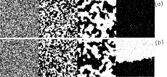
Figure 7: The two panels show the sequence of snapshots taken at $t=1,10,100,10^{5}$ with PBC (a) and APBC (b), after a quench at $T_{F}=1.8$, with $L=256$. Time increases from left to right. The first three configurations belong to the coarsening regime and show independence from BC. The last pair of configurations is morphologically similar to those in Fig. 6 and shows that at $t=10^{5}$ the system has equilibrated.

The configurations morphology, with large compact growing domains containing in their interior small patches of thermal fluctuations, suggests to generalize to the off-equilibrium regime the split of variables (56) by $s_{i}(t)=m_{\alpha(i,t)}+\psi_{i}(t)$, where $\alpha(i,t)$ is the label of the domain to which the site $i$ belongs at the time $t$. Then, as in Eq. (57), the correlation function separates into the sum of two contributions

$$C(r,\epsilon,t^{-1})=G_{\rm eq}(r,\epsilon)+D(r;\epsilon,t^{-1}),$$ (62)

where the first one is BC-independent, time-independent and identical to the analogous term appearing in Eqs. (53) and (57), because thermal fluctuations equilibrate quickly. The second contribution contains the correlations of the background variables and obeys scaling in the form

$$D(r,\epsilon,t^{-1})=\frac{m^{2}_{\alpha}}{r^{a}}F(r/R),$$ (63)

where $a=0$, due to the compactness of domains, the growth law $R(t)=t^{1/z}$ is the same of Eq. (14) with $z=2$ and the $\epsilon$ dependence has been factorized in the amplitude $m^{2}_{\alpha}$. Comparing with Eq. (36), we see that the same behavior as in the quench to $T_{c}$ is obtained, apart for the change of the exponents $z$ and $a$, and for the specific forms of the functions $F_{c}(x)$ and $F(x)$.

Figure 8: Collapse on the master curve of Eq. (47) of the data for $C(r,t^{-1},L^{-1})$ in the time regime $R\ll L$, system size $L=256$. PBC (black symbols) and APBC (empty symbols). The continuous line is the plot of the Ohta-Jasnow-Kawasaki function defined in Eq. (64).

The above statements are substantiated by the plot in Fig.8 of the numerical data for the equal-time correlation function, generated for a quench to $T_{F}/T_{c}=0.666$, which corresponds to $\epsilon=-0.9$, with $L=256$ and with both PBC and APBC. The APBC data have been circularly averaged to smooth out the anisotropy induced by the cylindrical BC. The good collapse of the data, in the time regime such that $R\ll L$, shows that for the chosen value of $T_{F}$ the thermal fluctuations contribution is negligible. Moreover, the master curve $F(x)$ compares well with the Otha-Jasnow-Kawasaki OJK approximate result

$$F(x)=\left(\frac{2}{\pi}\right)\arcsin(\gamma),\quad\gamma=\exp(-x^{2}/b),$$ (64)

where $b$ is a constant, as it is demonstrated by Fig.8. Therefore, the relaxation to below $T_{c}$ is not qualitatively different from the one to $T_{c}$. Both are coarsening processes and both do not depend on the imposed BC. Differences between the two are in the quantitative details, like the values of the $z$ exponent, the dimensionality of correlated clusters and the shape of the scaling functions. The implication is that also in the quench to below $T_{c}$ the system tends toward a critical state, because the time-dependent correlation length $R$ diverges, eventually yielding the time-asymptotic critical correlation function

$$C^{*}(r,\epsilon)=G_{\rm eq}(r,\epsilon)+\frac{m^{2}_{\alpha}}{r^{a}}.$$ (65)

It is then evident, according to the discussion made at the end of subsection VI.2, that this asymptotic form, which we emphasize once more is the same for both choices of BC, matches $C^{(a)}_{\rm eq}(r;\epsilon)$ but not $C^{(p)}_{\rm eq}(r;\epsilon)$. Finally, recalling that $a=0$, it is straightforward to see from Eq. (63) that the background susceptibility scales like

$$\chi(\epsilon,t^{-1})\sim R^{d},$$ (66)

in agreement with the result (61) for $\chi^{(a)}_{m}(\epsilon,L^{-1})$.

In conclusion, in the PBC case, as anticipated in the Introduction, the asymptotic state and the equilibrium one are remote one from the other, and the system may be regarded as remaining strongly out of equilibrium, because in the former one there are long-range correlations, which are absent in the second one. In the APBC case, instead, both the asymptotic and the equilibrium state are critical and with the same universal properties, hence the system equilibrates although with an infinite equilibration time, just as in the quench to $T_{c}$.

VI.4 Summary

So far we have shown that when the Ising model is quenched in the two-phase region, i.e. to below $T_{c}$ for $d=2$ and to $T_{F}=0$ for $d=1$, the APBC system equilibrates and the PBC one remains off equilibrium. The basic elements of the mechanism underlying this phenomenology are as follows:

1. To different BC, in principle, there correspond different statistical ensembles.

2. These ensembles become equivalent when the limits are taken according to the sequence: $L^{-1}\to 0$ first and then $t^{-1}\to 0$, for all temperatures $T_{F}$.

3. Instead, the ensembles may become non equivalent, depending on BC, when the limits are taken in the reverse sequence: $t^{-1}\to 0$ first and then $L^{-1}\to 0$ with $T_{F}<T_{c}$.

4. Equivalence fails with PBC because of ergodicity breaking, and holds with APBC since ergodicity is preserved.

5. Ergodicity breaking induces spontaneous symmetry breaking, which makes correlations short-ranged.

6. Instead, when ergodicity holds an unusual type of criticality sets in, with long-range correlations and compact correlated domains.

In the next section we shall show that this is not just a peculiarity of the Ising model, but that it is a more general phenomenon, since it takes place with the same characteristics also in the quench to below the critical point of the spherical model, without invoking the imposition of different types of BC. In fact, two different ensembles arise not from the choice of BC, which is taken to be the standard PBC one, but from enforcing the spherical constraint either sharply or smoothly. These ensembles turn out to be equivalent or non equivalent, just as in the Ising case, depending on the order of the $L^{-1}\to 0$ and $t^{-1}\to 0$ limits.

VII Spherical models

VII.1 Equilibrium

Let us briefly recall what the spherical model is about starting from equilibrium, which means that the $t^{-1}\to 0$ limit has been taken beforehand. Consider a classical paramagnet in the volume $V=L^{d}$ and with the energy function Ma

$${\cal H}(\boldsymbol{\varphi})=\int_{V}d\vec{r}\,\varphi(\vec{r})\left(-\frac{1}{2}\nabla^{2}\right)\varphi(\vec{r}),$$ (67)

where $\boldsymbol{\varphi}$ stands for a configuration of the local, continuous and unbounded spin variable $\varphi(\vec{r})$. PBC are understood throughout. Due to its bilinear character, the above Hamiltonian can be diagonalized by Fourier transform

$${\cal H}=\frac{1}{2V}\sum_{\vec{k}}k^{2}|\varphi_{\vec{k}}|^{2}.$$ (68)

In the spherical model (SM) of Berlin and Kac BK a coupling among the modes is induced by the imposition of an overall sharp constraint on the square magnetization density

$$\mathit{s}(\boldsymbol{\varphi})=\frac{1}{V}\int_{V}d\vec{r}\,\varphi^{2}(\vec{r})=\frac{1}{V^{2}}\sum_{\vec{k}}|\varphi_{\vec{k}}|^{2}=1.$$ (69)

Then, in thermal equilibrium the statistical ensemble is given by

$$P_{\textrm{SM}}(\boldsymbol{\varphi})=\frac{1}{Z_{\textrm{SM}}}e^{-\beta{\cal H}(\boldsymbol{\varphi})}\,\delta\left(\mathit{s}(\boldsymbol{\varphi})-1\right),$$ (70)

where $Z_{\textrm{SM}}$ is the partition function. A variant of the model, called the mean-spherical model (MSM) LW ; KT , is obtained by imposing the constraint in the mean: An exponential bias is introduced in place of the $\delta$ function

$$P_{\textrm{MSM}}(\boldsymbol{\varphi})=\frac{1}{Z_{\textrm{MSM}}}e^{-\beta[{\cal H}(\boldsymbol{\varphi})+\frac{\kappa}{2}{\cal S}(\boldsymbol{\varphi})]},$$ (71)

where ${\cal S}(\boldsymbol{\varphi})=V\mathit{s}(\boldsymbol{\varphi})$ and the parameter $\kappa$ must be so adjusted to satisfy the requirement

$$\langle\mathit{s}(\boldsymbol{\varphi})\rangle_{\textrm{MSM}}=1.$$ (72)

Although it is the common usage to refer to these as models, it should be clear from Eqs. (70) and (71) that we are dealing with two conjugate ensembles, distinguished by conserving or letting to fluctuate the density $\mathit{s}$.

In both models there exists a phase transition at the same critical temperature $T_{c}$, above which they are equivalent and below which they are not, which means that the nature of the low temperature phase is different. It is worth, here, to go in some detail CSZ because the point is quite illuminating on the equivalence or lack-of issue. Let us separate in $\mathit{s}$ the excitations from the ground-state contribution

$$\mathit{s}=\mathit{s}_{0}+\mathit{s}^{*},\quad\text{with}\quad\mathit{s}_{0}=\frac{1}{V^{2}}\varphi_{0}^{2},\quad\quad\mathit{s}^{*}=\frac{1}{V^{2}}\sum_{\vec{k}\neq 0}|\varphi_{\vec{k}}|^{2}.$$ (73)

Then, taking the average in either ensemble, from the spherical constraint follows the sum rule

$$\langle\mathit{s}_{0}\rangle+\langle\mathit{s}^{*}\rangle=1,$$ (74)

which must be satisfied at all temperatures and it is the motor of the transition. In fact, in the thermodynamic limit the excitations contribution is superiorly bounded CSZ by

$$\langle\mathit{s}^{*}\rangle\leq TB,$$ (75)

where $B$ is a dimensionality-dependent positive constant, which is finite for $d>2$ and diverges at $d=2$. Therefore, by enforcing the constraint (74) there remains defined the critical temperature

$$T_{c}=1/B,$$ (76)

above which the sum rule (74) is saturated without any contribution from $\langle\mathit{s}_{0}\rangle$, while below there must necessarily be a finite contribution from the ground state, yielding

$$\langle\mathit{s}_{0}\rangle=\left\{\begin{array}[]{ll}0,\;\;$for$,\;\;T\geq T_{c},\\ 1-T/T_{c},\;\;$for$,\;\;T<T_{c}.\end{array}\right.$$ (77)

Rewriting $\mathit{s}_{0}=\psi_{0}^{2}$, where $\psi_{0}$ is the density $\frac{1}{V}\varphi_{0}$, the question is how can there arise a finite contribution to $\langle\mathit{s}_{0}\rangle$ from this single degree of freedom and here is precisely where the two models differ. In the SM the sharp version (69) of the constraint introduces enough nonlinearity for the transition to take place by ordering. This means that ergodicity breaks down inducing the spontaneous breaking of the $\mathbb{Z}_{2}$ symmetry. Then, exactly like in the Ising model with PBC, the probability distribution of the magnetization density, that is of $\psi_{0}$, results from the mixture of the two pure ferromagnetic states

$$P_{\textrm{SM}}(\psi_{0})=\frac{1}{2}[\delta(\psi_{0}-m_{-})+\delta(\psi_{0}-m_{+})],$$ (78)

where $m_{\pm}=\pm\sqrt{1-T/T_{c}}$ is the spontaneous magnetization. Thus, in this case $\langle\mathit{s}_{0}\rangle_{SM}$ stands for the square of the spontaneous magnetization $m_{\pm}^{2}$. Instead, in the MSM ordering cannot take place, because the soft version (72) of the constraint leaves the statistics Gaussian. Neither ergodicity nor symmetry break down, as in the Ising APBC case. Then, below $T_{c}$, the only mean to build up the finite value of $\langle\mathit{s}_{0}\rangle_{MSM}$ needed to saturate the sum rule is by growing the fluctuations of $\psi_{0}$ through the spread out probability distribution given by

$$P_{\textrm{MSM}}(\psi_{0})=\frac{e^{-\frac{\psi_{0}^{2}}{2(1-T/T_{c})}}}{\sqrt{2\pi(1-T/T_{c})}}.$$ (79)

Therefore, now $\langle\mathit{s}_{0}\rangle_{MSM}$ stands for the macroscopic variance of $\psi_{0}$. Elsewhere EPL ; CCZ ; Zannetti ; Merhav ; Marsili , this type of transition, characterized by the fluctuations of an extensive quantity condensing into one microscopic component, has been referred to as condensation of fluctuations.

Figure 9: Magnetization distribution in the MSM model (a) and in the SM model (b), for $T<T_{c}$. The spikes in the right panel stand for $\delta$ functions.

Comparing Figs. 9 and 4, it is evident that the distributions are the same in the two cases where ergodicity breaks down, that is in the Ising model with PBC and in the SM. In the other two cases, Ising with APBC and MSM, the distributions are not superimposable but show the same physical phenomenon: ergodicity is preserved by developing macroscopic fluctuations of the magnetization, which remain finite in the thermodynamic limit and reveal the critical nature of the low temperature phase. In fact, in the MSM the structure factor, i.e. the Fourier transform of the correlation function, is given by CCZ

$$C_{\textrm{MSM}}(\vec{k})=\frac{T}{k^{2}}+m_{\pm}^{2}\delta(\vec{k}).$$ (80)

The two terms appearing above are the anolouges in Fourier space of those entering $C_{\rm eq}^{(a)}(r;\epsilon)$ in Eq. (60), with the correspondences

$$G_{\rm eq}(r;\epsilon)\longleftrightarrow\frac{T}{k^{2}},\quad\frac{m^{2}_{\alpha}}{r^{a}}\longleftrightarrow m_{\pm}^{2}\delta(\vec{k}).$$ (81)

Notice that, as it is well known, the thermal fluctuations contribution in the MSM is massless, i.e. is critical, at all temperatures below $T_{c}$. For simplicity, let us set $T=0$ in order to get rid on this contribution and to focus on the interesting one, which is the $\delta$-function term (Bragg peak). We emphasize that this is the Fourier transform of the background critical contribution with compact correlated clusters, just as the corresponding term in the Ising APBC case.

Finally, we point out that the $d=2$ case is analogous to Ising with $d=1$, because $T_{c}$ vanishes. However, for brevity, we shall not elaborate on this case here.

VII.2 Dynamics

Let us next consider the relaxation dynamics in the quench to $T_{F}=0$. In Ref. Fusco it was shown that, when the thermodynamic limit is taken first, the two models are equivalent at all times. Then, it is an exact result that the dynamical structure factor both for the SM and MSM is given by

$$C(\vec{k},t)=\Delta\left(1+\frac{2r^{2}_{0}}{R^{2}}\right)^{d/2}R^{d}\,e^{-(kR)^{2}},$$ (82)

where $C(\vec{k},0)=\Delta$ is the spatially uncorrelated initial condition at $T_{I}=\infty$, $R=\sqrt{2t}$ is the growth law for nonconserved dynamics and $r_{0}=1/(\sqrt{2}\Lambda)$ is the microscopic length related to the momentum cutoff $\Lambda$, which is imposed exponentially when integrating over $\vec{k}$ and is responsible for the corrections to scaling in the early regime. From the normalization condition at $t=0$

$$\int\frac{d^{d}k}{(2\pi)^{d}}\,C(\vec{k},0)e^{-k^{2}/\Lambda^{2}}=1,$$ (83)

there follows $\Delta=(2\sqrt{\pi})^{d}$. Inserting this into Eq. (82), with little algebra one can verify that indeed the normalization is satisfied at all times. Then, since the peak grows like $C(0,t)\sim R^{d}$, one can conclude that the asymptotic structure factor is the $\delta$ function

$$\lim_{t\to\infty}C(\vec{k},t)=C^{*}(\vec{k})=\delta(\vec{k}),$$ (84)

which matches the equilibrium Bragg peak (80) in the MSM. Since the growth of $R$ implies that the asymptotic state is critical and with compact correlated clusters, in the quench to below $T_{c}$ the MSM approaches equilibrium arbitrarily close, while the SM, which is not critical in the equilibrium state, remains permanently out of equilibrium.

In conclusion, going through all the items listed at the end of the previous section, one can check that perfect correspondence between Ising-PBC and SM on one side and Ising-APBC and MSM on the other is established.

VIII Concluding Remarks

In this paper we have addressed a problem which is of basic interest in the physics of slowly relaxing systems. Since slow relaxation means that equilibrium is not reached in the observable time scale, relevant questions are whether a criterion for equilibration, or for lack of, can be established and, if so, whether the nature of the equilibrium state can be inferred from the available dynamical information. Although the task of giving general answers to these questions is of formidable difficulty, we have shown that, at least in the restricted realm of phase-ordering systems, it is possible to arrive at some definite conclusions.

By analyzing the relaxation of the Ising model after temperature quenches, we have found that the system does or does not equilibrate, depending on whether the dynamics at the final temperature of the quench is ergodic or not. This has been established by investigating the dependence of the spin-spin correlation function upon the order of the large-time and thermodynamic limits, when different BC are imposed. The findings are that the APBC system equilibrates in all conditions, because the dynamics are ergodic at all temperatures, while the PBC system does not equilibrate for $T_{F}<T_{c}$, because that’s where ergodicity does not hold. These statements are strengthened and corroborated by exact analytical results from the quench of the spherical and mean spherical model, which reproduce very closely, although in a quite different context, the picture just outlined. We may then answer the first question asked at the beginning of the section by saying that it might take an infinite time to equilibrate, but nonetheless the system can get arbitrarily close to equilibrium if the dynamics are ergodic. Instead, if ergodicity is broken, and if the initial state is symmetric, the system does not get close to equilibrium, no matter how long is let to relax.

For what concerns the second question, the answer is that, yes, once it is established that the system approaches equilibrium, then the nature of the equilibrium state can be inferred from the dynamical information. Consider first the quench to $T_{c}$, in which case the time-dependent correlation function obeys the scaling form (36), while in the equilibrium state it decays according to the pure power law (35). It is then evident that the latter result can be reconstructed from the short distance behaviour, i.e. for $r\ll R$, at times finite but large enough to detect a clean scaling behaviour. The same procedure applies also in the case of the quench to below $T_{c}$ with APBC, where the background component of the correlation function is given by Eq. (63). Then, again the short distance approximation, which in this case is a constant term since $a=0$, reproduces correctly the form of the equilibrium critical correlation function.

Finally, let us comment on the nature of the line of critical points on the $\epsilon<0$ segment in the Ising APBC case. According to the view put forward in this paper, $t^{-1}$ is just another relevant parameter measuring the distance from criticality, on the same footing with $\epsilon$ and $L^{-1}$, so that these critical points control both statics and dynamics. In subsection VI.2 we have pointed out that the static critical exponents, defined with respect to $L^{-1}$, satisfy the hyperscaling relation $2\dot{\beta}+\dot{\gamma}=\dot{\nu}d$ for all $d$, suggesting that the upper critical dimension is at $d=\infty$. It is then interesting to note the concomitance with the fact that the Otha-Jasnow-Kawasaki approximate theory, which accounts well for the time dependent correlation function as shown in Fig.8, becomes exact in the $d\to\infty$ limit Bray .

- (1) R. G. Palmer, Adv. in Phys. 31, 669 (1982).
- (2) J. P. Bouchaud, L. F. Cugliandolo, J. Kurchan and M. Mezard, Out of equilibrium dynamics in spin glasses and other glassy systems, in Spin Glasses and Random Fields, edited by A. P. Young (World Scientific, Singapore, 1997); arXiv:cond-mat/9702070.
- (3) A. J. Bray, Adv. Phys. 43, 357 (1994).
- (4) S. Puri, in Kinetics of Phase Transitions, edited by S. Puri and V. Wadahawan (CRC Press, Boca Raton, FL, 2009).
- (5) M. Zannetti, in Kinetics of Phase Transitions, edited by S. Puri and V. Wadahawan (CRC Press, Boca Raton, FL, 2009).
- (6) M. Henkel and M. Pleimling, Non-Equilibrium Phase Transitions, Vol. 2, (Springer, Dordrecht, 2010).
- (7) A. Fierro, A. Coniglio and M. Zannetti, Phys. Rev. E 99, 042122 (2019).
- (8) G. Gallavotti, Riv. Nuovo Cimento 2, 133 (1972); Statistical Mechanics A Short Treatise, Springer-Verlag Berlin Heidelberg 1999.
- (9) T. Antal, M. Droz and Z. Rácz, J. Phys. A: Math. Gen. 37, 1465 (2004).
- (10) H. K. Janssen, B. Schaub and B. Schmittman, Z. Phys. B 73, 539 (1989).
- (11) A. Coniglio and W. Klein, J. Phys. A 13, 2775 (1980).
- (12) W. P. Kasteleyn and C. M. Fortuin, J. Phys. Soc. Japan Suppl. 26, 11 (1969).
- (13) A. Coniglio and A. Fierro, Correlated Percolation, in Encyclopedia of Complexity and Systems Science, Part 3, edited by R. A. Meyers (Springer-Verlag, New York, 2009), pp. 1596-1615; arXiv:1609.04160.
- (14) H. E. Stanley, Introduction to Phase Transitions and Critical Phenomena, Oxford Science Publications.
- (15) N. Goldenfeld, Lectures on Phase Transitions and the Renormalization Group, Addison-Wesley (1972).
- (16) A. J. Bray, J. Phys. A 22, L67 (1990); J. G. Amar and F. Family, Phys. Rev. A 41, 3258 (1990); B. Derrida, C. Godrèche and I. Yekutieli Phys. Rev. A, 44, 6241 (1991).
- (17) M. P. Nightingale and H. W. J. Blöte, Phys. Rev. Lett. 76, 4548 (1996).
- (18) S. K. Das, S. Roy, S. Majumder and S. Ahmad, Europhys. Lett. 97, 66006 (2012).
- (19) K. Binder, Z. Phys. B 43, 119 (1981).
- (20) A. D. Bruce, J. Phys. C: Solid State Phys. 14, 3667 (1981); ibidem 18, L873 (1985).
- (21) T. Ohta, D. Jasnow and K. Kawasaki, Phys. Rev. Lett. 49, 1223 (1982).
- (22) S. K. Ma, Modern Theory of Critical Phenomena, W A Benjamin (1976); D. J. Amit and V. Martín-Mayor, Field Theory, the Renormalization Group, and Critical Phenomena, World Scientific Singapore (2005).
- (23) T. H. Berlin and M. Kac, Phys. Rev. 86, 821 (1952).
- (24) H. W. Lewis and G. H. Wannier, Phys. Rev. 88, 682 (1952) and Phys. Rev. 90, 1131E (1953).
- (25) M. Kac and C. J. Thompson, J. Math. Phys. 18, 1650 (1977).
- (26) A. Crisanti, A. Sarracino and M. Zannetti, Phys. Rev. R 1, 023022 (2019).
- (27) M. Zannetti, EPL 111, 20004 (2015).
- (28) C. Castellano, F. Corberi and M. Zannetti, Phys. Rev. E 56, 4973 (1997).
- (29) F. Corberi, G. Gonnella, A. Piscitelli and M. Zannetti, J. Phys. A: Math. Theor. 46, 042001 (2013); M. Zannetti, F. Corberi and G. Gonnella, Phys. Rev. E 90, 012143 (2014); M.Zannetti, F. Corberi, G. Gonnella and A. Piscitelli, Commun. Theor. Phys. 62, 555 (2014).
- (30) N. Merhav and Y. Kafri, J. Stat. Mech. P02011 (2010).
- (31) M. Filiasi, G.Livan, M. Marsili. M. Peressi, E. Vesselli and E. Zarinelli, J. Stat. Mech. P09030 (2014); M. Filiasi, E. Zarinelli, E. Vesselli and M. Marsili, arXiv:1309.7795v1; L. Ferretti, M. Mamino and G. Bianconi, Phys. Rev. E 89, 042810 (2014).
- (32) N. Fusco and M. Zannetti, Phys. Rev. E 66, 066113 (2002).