Time-reversible and norm-conserving high-order integrators for the nonlinear time-dependent Schrödinger equation: Application to local control theory

Abstract

The explicit split-operator algorithm has been extensively used for solving not only linear but also nonlinear time-dependent Schrödinger equations. When applied to the nonlinear Gross-Pitaevskii equation, the method remains time-reversible, norm-conserving, and retains its second-order accuracy in the time step. However, this algorithm is not suitable for all types of nonlinear Schrödinger equations. Indeed, we demonstrate that local control theory, a technique for the quantum control of a molecular state, translates into a nonlinear Schrödinger equation with a more general nonlinearity, for which the explicit split-operator algorithm loses time reversibility and efficiency (because it has only first-order accuracy). Similarly, the trapezoidal rule (the Crank–Nicolson method), while time-reversible, does not conserve the norm of the state propagated by a nonlinear Schrödinger equation. To overcome these issues, we present high-order geometric integrators suitable for general time-dependent nonlinear Schrödinger equations and also applicable to nonseparable Hamiltonians. These integrators, based on the symmetric compositions of the implicit midpoint method, are both norm-conserving and time-reversible. The geometric properties of the integrators are proven analytically and demonstrated numerically on the local control of a two-dimensional model of retinal. For highly accurate calculations, the higher-order integrators are more efficient. For example, for a wavefunction error of $10^{-9}$, using the eighth-order algorithm yields a $48$-fold speedup over the second-order implicit midpoint method and trapezoidal rule, and $400000$-fold speedup over the explicit split-operator algorithm.

I Introduction

Nonlinear time-dependent Schrödinger equations contain, by definition, Hamiltonians that depend on the quantum state. Such state-dependent effective Hamiltonians appear in many areas of physics and chemistry. Examples include various nonlinear Schrödinger equations generated by the Dirac-Frenkel time-dependent variational principle, [1, 2, 3, 4] e.g., the equations of the multi-configurational time-dependent Hartree method,[5, 6, 7] and some numerical methods such as the short-iterative Lanczos algorithm.[8, 9, 10] Probably the best known nonlinear Schrödinger equations, however, are approximate equations for Bose-Einstein condensates,[11, 12] in which the Hamiltonian depends on the probability density of the quantum state. The dynamics of a Bose-Einstein condensate is often modeled by solving the celebrated Gross-Pitaevskii equation with a cubic nonlinearity.[13, 14, 15, 16, 17]

To solve this equation, several numerical schemes, such as the explicit split-operator algorithm or the time and spatial finite difference methods have been employed.[18, 19] These methods are of low accuracy (in time and/or space) and do not always preserve the geometric properties of the exact solution.[20] For example, the Crank–Nicolson finite difference method is geometric but exhibits only second-order convergence with respect to the spatial discretization. To remedy this, the explicit second-order split-operator algorithm,[21, 22, 23, 24] commonly used for the linear time-dependent Schrödinger equation, is a great alternative, as it conserves, in some cases, the geometric properties of the exact solution and has spectral accuracy in space. Unfortunately, this algorithm cannot be used for all types of nonlinear time-dependent Schrödinger equations. Indeed, in the case of the Gross-Pitaevskii equation, the algorithm is symmetric and, therefore, time-reversible only because the ordinary differential equation that must be solved when propagating the molecular state with the potential part of the Hamiltonian leaves the nonlinear term invariant in time.[18] We show here that for nonlinear terms of more general form, this algorithm becomes implicit. If this implicit nature is not taken into account and the explicit version is used, the algorithm loses its time reversibility and efficiency due to its low accuracy that is only of the first order in the time step.

An example of a situation, where a more general nonlinearity appears, is provided by local control theory (LCT). Introduced by Kosloff et al.,[25] LCT is a widely used approach to coherent control. In LCT, the pulse is computed on the fly, based on the instantaneous molecular state, in order to increase (or decrease) an expectation value of a specified operator. LCT has been successfully used to control various processes such as energy and population transfer,[25, 26, 27, 28] dissociation and association dynamics,[29, 30, 31, 32] direction of rotation in molecular rotors[33], and electron transfer.[34] Controlling quantum systems using LCT changes the nature of the time-dependent Schrödinger equation. Because the time dependence of the pulse is determined exclusively by the molecular state, the time-dependent Schrödinger equation becomes autonomous but nonlinear.

The nonlinear nature of LCT is often not acknowledged and the standard explicit split-operator algorithm[21] for linear time-dependent Schrödinger equations is used,[29, 30, 31, 32, 34] instead of its time-reversible, second-order, but implicit alternative. Most previous studies used LCT for applications that required neither high accuracy nor time reversibility, and therefore could rely on this approximate explicit integrator, which, as we show below, in the context of LCT, indeed has only first-order accuracy in the time step and is time-irreversible. Such an algorithm, however, would be very inefficient for highly accurate calculations, and could not be used at all if exact time reversibility were important. Because this failure of the explicit splitting algorithm in LCT is generic, while its success in the Gross-Pitaevskii equation is rather an exception, it is desirable to develop efficient high-order geometric integrators suitable for a general nonlinear time-dependent Schrödinger equation.

Recently, we presented high-order time-reversible geometric integrators for the nonadiabatic quantum dynamics driven by the linear time-dependent Schrödinger equation with both separable[35] and nonseparable[36] Hamiltonians. Here, we extend this work to the general nonlinear Schrödinger equation, in order to address the slow convergence and time irreversibility of the explicit split-operator algorithm.

The remainder of the study is organized as follows: In Sec. II, we define the nonlinear time-dependent Schrödinger equation, discuss its geometric properties, and explain how LCT leads to a nonlinear Schrödinger equation. In Sec. III, after demonstrating the loss of geometric properties by Euler methods, we describe how these geometric properties are recovered and accuracy increased to an arbitrary even order by symmetrically composing the implicit and explicit Euler methods. Then, we describe a general procedure to perform the implicit propagation and derive explicit expressions for the case of LCT. We also show the derivation of the approximate explicit split-operator algorithm for the nonlinear Schrödinger equation, explain how it loses time reversibility and briefly describe the dynamic Fourier method. Finally, in Sec. IV we numerically verify the convergence and geometric properties of the integrators by controlling, using LCT, either the population or energy transfer in a two-state two-dimensional model of retinal.[37]

II Nonlinear Schrödinger equation

The nonlinear time-dependent Schrödinger equation is the differential equation

$$i\hbar\frac{d}{dt}|\psi_{t}\rangle=\hat{H}(\psi_{t})|\psi_{t}\rangle,$$ (1)

describing the time evolution of the state $\psi_{t}$ driven by the nonlinear Hamiltonian operator $\hat{H}(\psi_{t})$, which depends on the state of the system. This dependence on $\psi_{t}$ is what distinguishes the equation from the linear Schrödinger equation. As the notation in Eq. (1) suggests, we shall always assume that while the operator $\hat{H}:\psi\mapsto\hat{H}(\psi)\psi$ is nonlinear, for each $\psi$ the operator $\hat{H}(\psi):\phi\mapsto\hat{H}(\psi)\phi$ is linear. We will also assume that $\hat{H}(\psi)$ has real expectation values $\langle\hat{H}(\psi)\rangle_{\phi}:=\langle\phi|\hat{H}(\psi)\phi\rangle$ in any state $\phi$, which for a linear operator implies that it is Hermitian, i.e., $\hat{H}(\psi)^{{\dagger}}=\hat{H}(\psi)$, or, more precisely, that for every $\psi$, $\phi$, $\chi$,

$$\langle\phi|\hat{H}(\psi)\chi\rangle=\langle\hat{H}(\psi)\phi|\chi\rangle.$$ (2)

A paradigm of a nonlinear Schrödinger equation is the Gross-Pitaevskii equation,[13, 14, 17] in position representation expressed as

$$i\hbar\partial_{t}\psi_{t}(q)=-\frac{\hbar^{2}}{2m}\nabla^{2}\psi_{t}(q)+V(q)\psi_{t}(q)+C|\psi_{t}(q)|^{2}\psi_{t}(q),$$

where the real coefficient $C$ is positive for a repulsive interaction and negative for an attractive interaction. This equation has a cubic nonlinearity and is useful, e.g., for approximate modeling of the dynamics of a Bose-Einstein condensate.[20] Many other examples are provided by the Dirac-Frenkel variational principle,[2, 1] which approximates the exact solution of a linear Schrödinger equation with Hamiltonian $\hat{H}$ by an optimal solution of a predefined, restricted form within a certain subset (called the approximation manifold) of the Hilbert space. This optimal solution $\psi_{t}$ satisfies the equation

$$\langle\delta\psi_{t}|(i\hbar d/dt-\hat{H})|\psi_{t}\rangle=0,$$ (3)

where $\delta\psi_{t}$ is an arbitrary variation in the approximation manifold. Equation (3) is equivalent to the nonlinear Eq. (1) with an effective state-dependent Hamiltonian

$$\hat{H}(\psi_{t})=\hat{P}(\psi_{t})\hat{H},$$

where $\hat{P}(\psi_{t})$ is the projection operator on the tangent space to the approximation manifold at the point $\psi_{t}$.[4, 38] (Note that in the very special case, where the projector does not depend on $\psi_{t}$, the resulting Schrödinger equation remains linear. This happens in the Galerkin method, in which $\psi_{t}$ is expanded in a finite, time-independent basis and the approximation manifold is a vector space.[4])

II.1 Geometric properties of the exact evolution operator

With initial condition $|\psi_{t_{0}}\rangle$ and assuming that $t\geq t_{0}$, Eq. (1) has the formal solution $|\psi_{t}\rangle=\hat{U}(t,t_{0};\psi)|\psi_{t_{0}}\rangle$ with the exact evolution operator given by

$$\hat{U}(t,t_{0};\psi):=\mathcal{T}\exp\left[-\frac{i}{\hbar}\int_{t_{0}}^{t}dt^{\prime}\hat{H}(\psi_{t^{\prime}})\right],$$ (4)

where the dependence of $\hat{U}$ on $\psi$ was added as an argument to emphasize the nonlinear character of Eq. (1). Expression (4) is obtained by solving the differential equation

$$i\hbar\frac{\partial}{\partial t}\hat{U}(t,t_{0};\psi)=\hat{H}(\psi_{t})\hat{U}(t,t_{0};\psi)$$

with initial condition $\hat{U}(t_{0},t_{0};\psi)=1$. The Hermitian adjoint of $\hat{U}(t,t_{0};\psi)$ is the operator

$$\hat{U}(t,t_{0};\psi)^{{\dagger}}=\mathcal{\bar{T}}\exp\left[\frac{i}{\hbar}\int_{t_{0}}^{t}dt^{\prime}\hat{H}(\psi_{t^{\prime}})\right]=\hat{U}(t,t_{0};\psi)^{-1},$$ (5)

where $\mathcal{\bar{T}}$ denotes the reverse time-ordering operator.

The nonlinearity of $\hat{H}$ leads to the loss of some geometric properties, even if Eq. (1) is solved exactly. Indeed, since the Hamiltonian is nonlinear, the exact evolution operator is also nonlinear.

An operator $\hat{U}$ is said to preserve the inner product (or to be unitary) if $\langle\hat{U}\psi|\hat{U}\phi\rangle=\langle\psi|\phi\rangle$. The exact evolution operator does not preserve the inner product because

$$\langle\psi_{t}|\phi_{t}\rangle =\langle\hat{U}(t,t_{0};\psi)\psi_{t_{0}}|\hat{U}(t,t_{0};\phi)\phi_{t_{0}}\rangle$$

$$=\langle\psi_{t_{0}}|\hat{U}(t,t_{0};\psi)^{\dagger}\hat{U}(t,t_{0};\phi)\phi_{t_{0}}\rangle$$

$$=\langle\psi_{t_{0}}|\hat{U}(t,t_{0};\psi)^{-1}\hat{U}(t,t_{0};\phi)\phi_{t_{0}}\rangle$$

$$\neq\langle\psi_{t_{0}}|\phi_{t_{0}}\rangle$$ (6)

if $\psi_{t_{0}}\neq\phi_{t_{0}}$, where we used the property (5) of the Hermitian adjoint of $\hat{U}$ to obtain the third line. The exact nonlinear evolution operator is, therefore, not symplectic because it does not preserve the associated symplectic two-form[4]

$$\omega(\psi,\phi):=-2\hbar\operatorname{Im}\langle\psi|\phi\rangle.$$ (7)

The nonlinear evolution does not conserve energy

$$E_{t}:=\langle\hat{H}\left(\psi_{t}\right)\rangle_{\psi_{t}}=\langle\psi_{t}|\hat{H}(\psi_{t})\psi_{t}\rangle,$$

since

$$\frac{dE_{t}}{dt} =\langle\dot{\psi}_{t}|\hat{H}(\psi_{t})|\psi_{t}\rangle+\langle\psi_{t}|\frac{d}{dt}\hat{H}(\psi_{t})|\psi_{t}\rangle$$

$$\qquad+\langle\psi_{t}|\hat{H}(\psi_{t})|\dot{\psi}_{t}\rangle$$

$$=\langle d\hat{H}(\psi_{t})/dt\rangle_{\psi_{t}}\neq 0,$$ (8)

where the first and third terms in the intermediate step cancel each other because $\psi_{t}$ satisfies the nonlinear Schrödinger equation (1). Note, however, that in special cases, such as the Gross-Pitaevskii equation, there exist modified energy functionals that are conserved.[20]

An operator $\hat{U}$ is said to conserve the norm $\|\psi\|:=\langle\psi|\psi\rangle^{1/2}$ if $\|\hat{U}\psi\|=\|\psi\|$. The exact nonlinear evolution operator $\hat{U}\equiv\hat{U}(t,t_{0};\psi)$ conserves the norm because

$$\|\psi_{t}\|^{2} =\|\hat{U}\psi_{t_{0}}\|^{2}=\langle\hat{U}\psi_{t_{0}}|\hat{U}\psi_{t_{0}}\rangle$$

$$=\langle\psi_{t_{0}}|\hat{U}^{\dagger}\hat{U}\psi_{t_{0}}\rangle=\langle\psi_{t_{0}}|\psi_{t_{0}}\rangle=\|\psi_{t_{0}}\|^{2},$$ (9)

where we used relation (5).

In the theory of dynamical systems, an adjoint $\hat{U}(t,t_{0};\psi)^{\ast}$ of $\hat{U}(t,t_{0};\psi)$ is defined as the inverse of the evolution operator taken [in contrast to the Hermitian adjoint (5)] with a reversed time flow:

$$\hat{U}(t,t_{0};\psi)^{\ast}:=\hat{U}(t_{0},t;\psi)^{-1}.$$ (10)

An operator $\hat{U}(t,t_{0};\psi)$ is called symmetric if it is equal to its adjoint, i.e., if $\hat{U}(t,t_{0};\psi)=\hat{U}(t,t_{0};\psi)^{\ast}$. A symmetric operator is also time-reversible because propagating a molecular state $\psi_{t_{0}}$ forward to time $t$ and then backward to time $t_{0}$ yields $\psi_{t_{0}}$ again, i.e.,

$$\hat{U}(t_{0},t;\psi)\hat{U}(t,t_{0};\psi)\psi_{t_{0}}$$

$$=\hat{U}(t_{0},t;\psi)\hat{U}(t,t_{0};\psi)^{\ast}\psi_{t_{0}}$$

$$=\hat{U}(t_{0},t;\psi)\hat{U}(t_{0},t;\psi)^{-1}\psi_{t_{0}}=\psi_{t_{0}}.$$ (11)

For the operator (4), the reverse evolution operator is given by the anti-time-ordered exponential

$$\hat{U}(t_{0},t;\psi):=\bar{\mathcal{T}}\exp\left[-\frac{i}{\hbar}\int_{t}^{t_{0}}dt^{\prime}\hat{H}(\psi_{t^{\prime}})\right]$$ (12)

and, therefore, the adjoint is

$$\hat{U}(t,t_{0};\psi)^{\ast} =\left\{\bar{\mathcal{T}}\exp\left[-\frac{i}{\hbar}\int_{t}^{t_{0}}dt^{\prime}\hat{H}(\psi_{t^{\prime}})\right]\right\}^{-1}$$

$$=\mathcal{T}\exp\left[\frac{i}{\hbar}\int_{t}^{t_{0}}dt^{\prime}\hat{H}(\psi_{t^{\prime}})\right]$$

$$=\mathcal{T}\exp\left[-\frac{i}{\hbar}\int_{t_{0}}^{t}dt^{\prime}\hat{H}(\psi_{t^{\prime}})\right]=\hat{U}(t,t_{0};\psi).$$ (13)

This shows that the exact evolution operator (4) is symmetric and time-reversible.

Finally, a time evolution is said to be stable if for every $\epsilon>0$ there is a $\delta>0$ such that the distance between two states satisfies the condition

$$\|\psi_{t_{0}}-\phi_{t_{0}}\|<\delta\implies\|\psi_{t}-\phi_{t}\|<\epsilon\text{ for all }t>t_{0}.$$ (14)

Although the exact evolution conserves the norm, because it does not conserve the inner product, we cannot, in general, say anything about preserving the distance:

$$\|\psi_{t}-\phi_{t}\|^{2} =\|\psi_{t}\|^{2}+\|\phi_{t}\|^{2}-2\operatorname{Re}\langle\psi_{t}|\phi_{t}\rangle$$

$$=\|\psi_{t_{0}}\|^{2}+\|\phi_{t_{0}}\|^{2}-2\operatorname{Re}\langle\psi_{t}|\phi_{t}\rangle$$

$$=\|\psi_{t_{0}}-\phi_{t_{0}}\|^{2}+2\operatorname{Re}\left(\langle\psi_{t_{0}}|\phi_{t_{0}}\rangle-\langle\psi_{t}|\phi_{t}\rangle\right)$$

$$\neq\|\psi_{t_{0}}-\phi_{t_{0}}\|^{2}.$$ (15)

Moreover, since the sign of the real part of the difference of the inner products can be arbitrary, we cannot deduce anything about stability.

II.2 Nonlinear character of local control theory

We now show that the local coherent control of the time evolution of a quantum system with an electric field provides another example of a nonlinear Schrödinger equation. The quantum state $|\psi_{t}\rangle$ of a system interacting with an external time-dependent electric field $\vec{E}(t)$ evolves according to the linear time-dependent Schrödinger equation

$$i\hbar\frac{d}{dt}|\psi_{t}\rangle=\hat{H}(t)|\psi_{t}\rangle$$ (16)

with a time-dependent Hamiltonian

$$\hat{H}(t):=\hat{H}_{0}+\hat{V}_{\text{int}}(t),$$ (17)

equal to the sum of the Hamiltonian $\hat{H}_{0}$ of the system in the absence of the field and the interaction potential $\hat{V}_{\text{int}}(t)$. Within the electric-dipole approximation,[39] the interaction potential is

$$\hat{V}_{\text{int}}(t):=-\vec{\mu}(\hat{q})\cdot\vec{E}(t),$$ (18)

where the vector function $\vec{\mu}(\hat{q})$ of the position operator $\hat{q}$ denotes the electric-dipole operator of the system. Direct integration of Eq. (16) with initial condition $|\psi_{t_{0}}\rangle$ leads to the formal solution $|\psi_{t}\rangle=\hat{U}(t,t_{0})|\psi_{t_{0}}\rangle$ with the exact evolution operator given by the time-ordered exponential

$$\hat{U}(t,t_{0}):=\mathcal{T}\exp\left[-\frac{i}{\hbar}\int_{t_{0}}^{t}dt^{\prime}\hat{H}(t^{\prime})\right].$$ (19)

This exact evolution operator has many important geometric properties: it is linear, unitary, symmetric, time-reversible, and stable.[40, 41, 4, 42] Because it is unitary, the evolution operator conserves the norm as well as the inner product and symplectic structure.[4] However, since the Hamiltonian is time-dependent, the Schrödinger equation (16) is a nonautonomous differential equation,[42] and as a consequence, does not conserve energy. For a more detailed presentation and discussion of the above properties, we refer the reader to Ref. 36.

Contrary to Eq. (18), the electric field used in LCT, called control field and denoted by $\vec{E}_{\text{LCT}}(t)$, is not known explicitly as a function of time. Instead, it is chosen “on the fly” according to the current state $|\psi_{t}\rangle$ of the system, in order to increase or decrease the expectation value $\langle\hat{O}\rangle_{{\psi}_{t}}:=\langle\psi_{t}|\hat{O}|\psi_{t}\rangle$ of a particular operator $\hat{O}$ in the state $|\psi_{t}\rangle$. More precisely, the control field is computed so that the time derivative of the expectation value,

$$\frac{d\langle\hat{O}\rangle_{\psi_{t}}}{dt} =\frac{i}{\hbar}\langle[\hat{H}(t),\hat{O}]\rangle_{\psi_{t}}$$

$$=\frac{i}{\hbar}\left\{\langle[\hat{H}_{0},\hat{O}]\rangle_{\psi_{t}}-\vec{E}_{\text{LCT}}(t)\cdot\langle[\hat{\vec{\mu}},\hat{O}]\rangle_{\psi_{t}}\right\},$$ (20)

remains positive or negative at all times. If the operator $\hat{O}$ commutes with the system’s Hamiltonian $\hat{H}_{0}$, this goal is achieved by using the field

$$\vec{E}_{\text{LCT}}(t)\equiv\vec{E}_{\text{LCT}}(\psi_{t}):=\pm\lambda i\langle[\hat{\vec{\mu}},\hat{O}]\rangle_{\psi_{t}}^{\ast}=\mp\lambda i\langle[\hat{\vec{\mu}},\hat{O}]\rangle_{\psi_{t}},$$ (21)

where $\lambda>0$ is a parameter which scales the intensity of the control field and the sign in Eq. (21) is chosen according to whether one wants to increase or decrease $\langle\hat{O}\rangle_{\psi_{t}}$. This claim is proven by inserting the definition (21) of $\vec{E}_{\text{LCT}}(t)$ into Eq. (20), which yields

$$\frac{d\langle\hat{O}\rangle_{\psi_{t}}}{dt}=\frac{i}{\hbar}\langle[\hat{H}_{0},\hat{O}]\rangle_{\psi_{t}}\pm\frac{\lambda}{\hbar}\|\langle[\hat{\vec{\mu}},\hat{O}]\rangle_{\psi_{t}}\|^{2}$$ (22)

for the derivative of the expectation value. This equation confirms that a strictly increasing or strictly decreasing evolution of $\langle\hat{O}\rangle_{\psi_{t}}$ is guaranteed only if $[\hat{H}_{0},\hat{O}]=0$, largely reducing the choice of operators $\hat{O}$ whose expectation values we can control monotonically.

The left-hand side of Eq. (21) suggests that the control field can be either viewed as a function of time or a function of the molecular state [i.e., $\vec{E}_{\text{LCT}}(t)\equiv\vec{E}_{\text{LCT}}(\psi_{t})$]. More precisely, the control field does not depend on time explicitly but only implicitly through the dependence on $\psi_{t}$. Therefore, the time-dependent Schrödinger equation changes from a nonautonomous linear to an autonomous nonlinear differential equation.[42] By acknowledging this nonlinear character, the interaction potential from Eq. (18) becomes

$$\hat{V}_{\text{LCT}}(\psi_{t}):=-\hat{\vec{\mu}}\cdot\vec{E}_{\text{LCT}}(\psi_{t})$$ (23)

and Eq. (16) becomes an example of a nonlinear time-dependent Schrödinger equation (1) with Hamiltonian operator $\hat{H}(\psi):=\hat{H}_{0}+\hat{V}_{\text{LCT}}(\psi)$.

III Geometric integrators for the nonlinear Schrödinger equation

Numerical propagation methods for solving the nonlinear equation (1) obtain the state at time $t+\Delta t$ from the state at time $t$ by using the relation

$$|\psi_{t+\Delta t}\rangle=\hat{U}_{\text{appr}}(t+\Delta t,t;\psi)|\psi_{t}\rangle,$$ (24)

where $\Delta t$ denotes the numerical time step and $\hat{U}_{\text{appr}}(t+\Delta t,t;\psi)$ is an approximate nonlinear evolution operator depending on $\psi$. By construction, all propagation methods converge to the exact solution in the limit $\Delta t\rightarrow 0$. As the exact operator, these approximate evolution operators $\hat{U}_{\text{appr}}(t+\Delta t,t;\psi)$ are, therefore, nonlinear and conserve neither the inner product nor the symplectic form. Moreover, nothing can be said about their stability in general. However, some integrators may lose even the remaining geometric properties of the exact evolution: norm conservation, symmetry, and time reversibility. In this section, we simply state the properties that are lost by different methods; detailed proofs are provided in Appendix A.

III.1 Loss of geometric properties by Euler methods

The simplest methods, applicable to both separable and nonseparable and both linear and nonlinear Hamiltonian operators, are the explicit and implicit Euler[4, 41] methods which approximate the exact evolution operator, respectively, as

$$\hat{U}_{\text{expl}}(t+\Delta t,t;\psi_{t}) :=1-i\hat{H}(\psi_{t})\Delta t/\hbar,$$ (25)

$$\hat{U}_{\text{impl}}(t+\Delta t,t;\psi_{t+\Delta t}) :=[1+i\hat{H}(\psi_{t+\Delta t})\Delta t/\hbar]^{-1}.$$ (26)

Both methods are only first-order in the time step and, therefore, very inefficient. Moreover, both Euler methods lose the norm conservation, symmetry, and time reversibility of the exact evolution operator.

III.2 Recovery of geometric properties and increasing accuracy by composition

Composing the implicit and explicit Euler methods yields, depending on the order of composition, either the implicit midpoint method

$$\hat{U}_{\text{mid}}(t+\Delta t,t;\psi_{t+\Delta t/2})\\ :=\hat{U}_{\text{expl}}(t+\Delta t,t+\Delta t/2;\psi_{t+\Delta t/2})\\ \times\hat{U}_{\text{impl}}(t+\Delta t/2,t;\psi_{t+\Delta t/2})$$ (27)

or the trapezoidal rule (or Crank–Nicolson method)

$$\hat{U}_{\text{trap}}(t+\Delta t,t;\psi)\\ :=\hat{U}_{\text{impl}}(t+\Delta t,t+\Delta t/2;\psi_{t+\Delta t})\\ \times\hat{U}_{\text{expl}}(t+\Delta t/2,t;\psi_{t}).$$ (28)

Both methods are second-order, symmetric, and time-reversible regardless of the size of the time step.[42, 36] Although the trapezoidal rule conserves the norm of a state evolved with a time-independent linear Hamiltonian,[36] it loses this property when the Hamiltonian is time-dependent or nonlinear (which results, as we have seen, in an implicit time dependence). In contrast, the implicit midpoint method remains norm-conserving in all cases.

Because they are symmetric, both methods can be further composed using symmetric composition schemes[4, 42, 43, 44, 45, 46, 36] in order to obtain integrators of arbitrary even order of accuracy in the time step. Indeed, every symmetric method $\hat{U}_{p}$ of an even order $p$ generates a method $\hat{U}_{p+2}$ of order $p+2$ if it is symmetrically composed as

$$\hat{U}_{p+2}(t+\Delta t,t;\psi):=\hat{U}_{p}(t+\gamma_{M}\Delta t,t+\gamma_{M-1}\Delta t;\psi)\\ \quad\cdots\hat{U}_{p}(t+\gamma_{1}\Delta t,t;\psi),$$ (29)

where $M$ is the number of composition steps, $\gamma_{1},\dots,\gamma_{M}$ are real composition coefficients which satisfy the relations $\sum_{n=1}^{M}\gamma_{n}=1$, $\gamma_{M+1-n}=\gamma_{n},$ and a more-involved third condition[42] guaranteeing the increase in the order of accuracy.

The simplest composition methods that are used here are the triple-jump [43] and Suzuki’s fractal[44] with $M=3$ and $M=5$, respectively. Both are recursive and able to generate integrators of arbitrary even orders of accuracy. Sixth, eighth, and tenth-order integrators can also be obtained with nonrecursive composition methods[45, 46] which require fewer composition steps and also minimize their magnitude. These composition methods are therefore more efficient than the triple-jump and Suzuki’s fractal and will be referred to as “optimal” compositions. For more details on symmetric compositions, see Ref. 36, where they were applied to a linear Schrödinger equation.

III.3 Solving the implicit step in a general nonlinear Schrödinger equation

The implicit Euler method requires implicit propagation because its integrator [see Eq. (26)] depends on the result of the propagation, i.e., $\psi_{t+\Delta t}$. In the implicit Euler method, $\psi_{t+\Delta t}$ is obtained by solving the nonlinear system

$$\hat{U}_{\text{impl}}(t+\Delta t,t;\psi_{t+\Delta t})^{-1}|\psi_{t+\Delta t}\rangle=|\psi_{t}\rangle,$$ (30)

which can be written as $f(\psi_{t+\Delta t})=0$ with the nonlinear functional

$$f(\psi): =\hat{U}_{\text{impl}}(\psi)^{-1}\psi-\psi_{t}$$

$$=[\hat{1}+i\hat{H}(\psi)\Delta t/\hbar]\psi-\psi_{t}.$$ (31)

A nonlinear system $f(\psi)=0$ can be solved with the iterative Newton-Raphson method, which computes, until convergence is obtained, the solution $\psi^{(k+1)}$ at iteration $k+1$ from $\psi^{(k)}$ using the relation

$$\psi^{(k+1)}=\psi^{(k)}-\hat{J}(\psi^{(k)})^{-1}f(\psi^{(k)}),$$ (32)

where $\hat{J}:=\frac{\delta}{\delta\psi}f(\psi)$ is the Jacobian of the nonlinear functional $f(\psi)$.

If the initial guess $\psi^{(0)}$ is close enough to the exact solution of the implicit propagation, the Newton-Raphson iteration (32) is a contraction mapping and by the fixed-point theorem is guaranteed to converge. We use as the initial guess the result of propagating $\psi_{t}$ with the explicit Euler method [Eq. (25)]. Note that this initial guess is sufficiently close to the implicit solution only if the time step is small. If the time step is too large, the difference between the explicit and implicit propagations becomes too large for the algorithm to converge and no solution can be obtained.

Equation (32) requires computing the inverse of the Jacobian which is an expensive task. It is preferable to avoid this inversion by computing each iteration as

$$\psi^{(k+1)}=\psi^{(k)}+\delta\psi^{(k)}$$ (33)

where $\delta\psi^{(k)}$ solves the linear system

$$\hat{J}(\psi^{(k)})\delta\psi^{(k)}=-f(\psi^{(k)}).$$ (34)

We solve this linear system by the generalized minimal residual method [47, 48, 49], an iterative method based on the Arnoldi process[50, 51] (see Sec. I of the supplementary material for a detailed presentation of this algorithm).

The procedure presented for solving the implicit propagation is applicable to any nonlinear system whose Jacobian is known analytically. Therefore, the integrators proposed in Secs. III.1 and III.2 can be employed for solving any nonlinear time-dependent Schrödinger equation of the form of Eq. (1), i.e., with a Hamiltonian $\hat{H}(\psi_{t})$ depending on the state of the system.

To sum up, each implicit propagation step, given by the evolution operator (26), is performed as follows:

1. Compute the initial guess $\psi^{(0)}$ using the explicit Euler method [see Eq. (25)]. Choose an error threshold $\varepsilon$ and a maximum iteration number $m$.

2. For $k=0,1,\dots,m-1$, Do:

3. Compute $\delta\psi^{(k)}$ by solving the linear system shown in Eq. (34).

4. Compute a new approximate solution $\psi^{(k+1)}$ using Eq. (33).

5. If $\|f(\psi^{(k+1)})\|\leq\varepsilon$, take $\psi^{(k+1)}$ as the solution of the implicit step.

6. End Do. The algorithm fails when $k=m$ and no approximate solution has been found.

III.4 Solving the implicit step in LCT

In the case of LCT,

$$\hat{U}_{\text{LCT,impl}}(\psi)^{-1}=\hat{1}+i\Delta t[\hat{H}_{0}+\hat{V}_{\text{LCT}}(\psi)]/\hbar,$$

and the Jacobian of the nonlinear functional (31) is

$$\hat{J}(\psi) =\frac{\delta}{\delta\psi}\left[\hat{U}_{\text{LCT,impl}}(\psi)^{-1}\right]\psi+\hat{U}_{\text{LCT,impl}}(\psi)^{-1}\hat{1}$$

$$=\frac{i}{\hbar}\Delta t\frac{\delta}{\delta\psi}\left[\hat{V}_{\text{LCT}}(\psi)\right]\psi+\hat{U}_{\text{LCT,impl}}(\psi)^{-1}$$

$$=\frac{i}{\hbar}\Delta t\hat{V}_{\text{LCT}}(\psi)+\hat{1}+\frac{i}{\hbar}\Delta t\left[\hat{H}_{0}+\hat{V}_{\text{LCT}}(\psi)\right]$$

$$=\hat{1}+i\Delta t[\hat{H}_{0}+2\hat{V}_{\text{LCT}}(\psi)]/\hbar.$$ (35)

To obtain the third row of Eq. (35), we used $\frac{\delta}{\delta\psi}[\hat{V}_{\text{LCT}}(\psi)]\psi=\hat{V}_{\text{LCT}}(\psi)$, where the generalized complex derivative[52] of the interaction potential is given by the bra vector

$$\frac{\delta}{\delta\psi}\hat{V}_{\text{LCT}}(\psi)=-\hat{\vec{\mu}}\cdot\frac{\delta}{\delta\psi}\vec{E}_{\text{LCT}}(\psi)=\mp\lambda i\hat{\vec{\mu}}\cdot\langle\psi|[\hat{\vec{\mu}},\hat{O}].$$ (36)

III.5 Approximate application of the explicit split-operator algorithm to the nonlinear Schrödinger equation

The algorithms that we described above apply to Hamiltonians that are not only nonlinear but also nonseparable, i.e., to Hamiltonians $\hat{H}$ which cannot be written as a sum $\hat{H}=T(\hat{p})+V(\hat{q})$ of a momentum-dependent kinetic term and position-dependent potential term. If the time-dependent Schrödinger equation is linear and its Hamiltonian is separable, the midpoint method remains implicit, but the split-operator algorithms and their compositions yield explicit high-order integrators satisfying most geometric properties (except for the conservation of energy). In the case of LCT, if $\hat{H}_{0}$ is separable, so is the total Hamiltonian, which can be written as $\hat{H}(\psi)=\hat{T}+\hat{V}_{\text{tot}}(\psi)$, where $\hat{V}_{\text{tot}}(\psi):=\hat{V}_{0}+\hat{V}_{\text{LCT}}(\psi)$ is the sum of the system’s and interaction potential energy operators. It is, therefore, tempting to use the split-operator algorithm, with the hope of obtaining an efficient explicit integrator.

More generally, let us assume that the Hamiltonian operator in the general nonlinear Schrödinger equation (1) can be separated as

$$\hat{H}(\psi)=T(\hat{p})+V_{\text{tot}}(\hat{q},\psi).$$

The approximate evolution operator is given by

$$\hat{U}_{\text{TV}}(t+\Delta t;t,\psi_{t}):=e^{-i\hat{T}\Delta t/\hbar}e^{-i\hat{V}_{\text{tot}}(\psi_{t})\Delta t/\hbar}$$ (37)

in the TV split-operator algorithm and by

$$\hat{U}_{\text{VT}}(t+\Delta t;t,\psi_{t+\Delta t}):=e^{-i\hat{V}_{\text{tot}}(\psi_{t+\Delta t})\Delta t/\hbar}e^{-i\hat{T}\Delta t/\hbar}$$ (38)

in the VT split-operator algorithm. These integrators are norm-conserving but only first-order and time-irreversible. From their definitions (37) and (38), it follows immediately that the TV and VT algorithms are adjoints[35] of each other and require, respectively, explicit and implicit propagations. In analogy to the implicit midpoint algorithm from Sec. III.2, a second-order method is obtained by composing the two adjoint methods to obtain the TVT split-operator algorithm

$$\hat{U}_{\text{TVT}}(t+\Delta t;t,\psi_{t+\Delta t/2})\\ :=\hat{U}_{\text{TV}}(t+\Delta t;t+\Delta t/2,\psi_{t+\Delta t/2})\\ \times\hat{U}_{\text{VT}}(t+\Delta t/2;t,\psi_{t+\Delta t/2}),$$ (39)

or the VTV split-operator algorithm if the order of composition is reversed. Both TVT and VTV algorithms are norm-conserving, symmetric, and time-reversible. However, these geometric properties are only acquired if the implicit part, i.e., the propagation with the VT algorithm (39) is performed exactly. This requires solving a nonlinear system, which can be performed using the Newton-Raphson method, as described in Sec. III.3. This, however, implies abandoning the explicit nature of the split-operator algorithm, which is one of its main advantages over implicit methods for solving linear Schrödinger equations.

The nonlinearity of Eq. (1) is often not acknowledged. As a consequence, the implicit character of Eqs. (38)-(39) is not taken into account and explicit alternatives of these algorithms are used. For example, instead of using $\psi_{t+\Delta t}$ in the VT algorithm (i.e., performing the implicit propagation exactly), the state $\psi_{t,\hat{T}\Delta t}:=e^{-i\hat{T}\Delta t/\hbar}\psi_{t}$ obtained after the kinetic propagation is often used to perform the potential propagation.After composition with the TV algorithm, it yields the approximate explicit TVT split-operator algorithm

$$\hat{U}_{\text{expl TVT}}(t+\Delta t;t,{\psi_{t,\hat{T}\Delta t/2}})\\ :=\hat{U}_{\text{TV}}(t+\Delta t;t+\Delta t/2,{\psi_{t,\hat{T}\Delta t/2}})\\ \times\hat{U}_{\text{VT}}(t+\Delta t/2;t,{\psi_{t,\hat{T}\Delta t/2}}).$$ (40)

This approximate explicit integrator can be used to successfully perform LCT but, because it depends on $\psi_{t,\hat{T}\Delta t/2}$ instead of $\psi_{t+\Delta t/2}$, it is not time-reversible and achieves only first-order accuracy. Like the approximate explicit TVT algorithm, any other explicit algorithm cannot perform the implicit step of the $\hat{U}_{VT}$ algorithm exactly and, therefore, cannot be time-reversible. Yet, the approximate explicit algorithm does conserve norm (see Appendix A for proofs of the geometric properties).

III.6 Dynamic Fourier method

To propagate the molecular state using the algorithms presented in Sec. III, an efficient way of evaluating the action of an operator on the molecular state $\psi_{t}$ is needed. For this, we use the dynamic Fourier method,[21, 24, 22, 23] which is applicable to operators that are sums of products of operators of the form $f(\hat{x})$, where $\hat{x}$ denotes either the momentum operator $\hat{p}$ or position operator $\hat{q}$. The computation of $f(\hat{x})\psi_{t}$ is then performed easily, by pointwise multiplication, in the $x$-representation, in which $\hat{x}$ is diagonal. Whenever required, the representation of $\psi_{t}$ is changed by Fourier transform. In the numerical examples below, we used the Fastest Fourier Transform in the West 3 (FFTW3) library [53] to perform all of the Fourier transforms. Unlike finite difference methods, the Fourier method shows exponential convergence with respect to the number of grid points (see Figs. S1 and S2 of the supplementary material).

IV Numerical examples

We tested the general integrators for the nonlinear Schrödinger equation, presented in Sec. III, by using them for the local control of a two-dimensional two-state diabatic model of retinal taken from Ref. 37. The model describes the cis-trans photo-induced isomerization of retinal—an ultrafast reaction mediated by a conical intersection and the first event occurring in the biological process of vision. The two vibrational modes of the model are the reaction coordinate $\theta$, an angle describing the torsional motion of the retinal molecule, and a vibronically active coupling mode $q_{c}$. In the diabatic representation, the Hamiltonian of the system in the absence of the field,

$$\hat{\mathbf{H}}_{0}=\hat{T}\mathbf{1}+\begin{pmatrix}V_{11}(\hat{q}_{c},\hat{\theta})&V_{12}(\hat{q}_{c})\\ V_{21}(\hat{q}_{c})&V_{22}(\hat{q}_{c},\hat{\theta})\end{pmatrix},$$ (41)

is separable into a sum of the kinetic energy operator

$$\hat{T}=-\frac{1}{2}\omega\frac{\partial^{2}}{\partial q_{c}^{2}}-\frac{1}{2}m^{-1}\frac{\partial^{2}}{\partial\theta^{2}}$$ (42)

and potential energy operator with components

$$V_{11}(q_{c},\theta) =\frac{1}{2}\omega q_{c}^{2}+\frac{1}{2}W_{1}\left[1-\cos(\theta)\right],$$ (43)

$$V_{22}(q_{c},\theta) =\frac{1}{2}\omega q_{c}^{2}+\chi_{2}q_{c}+E_{2}-\frac{1}{2}W_{2}\left[1-\cos(\theta)\right],$$ (44)

$$V_{12}(q_{c}) =V_{21}(q_{c})=\xi q_{c}.$$ (45)

Here (all parameters are in eV units), $\omega=0.19$ is the vibrational frequency of the coupling mode, $m^{-1}=4.84\cdot 10^{-4}$ is the inverse mass of the reaction coordinate, $W_{1}=3.6$ and $W_{2}=1.09$ determine the depth of the well in the reaction coordinate for the ground and excited electronic states, respectively, $\chi_{2}=0.1$ is the gradient of the linear perturbation in the excited electronic state, $E_{2}=2.48$ determines the maximum of the excited electronic state in the reaction coordinate, and $\xi=0.19$ is the gradient of the linear coupling between the two electronic states. The two diabatic potential energy surfaces (43) and (44) are displayed in Fig. S3 of the supplementary material.

Note that, to distinguish nuclear, electronic, and molecular operators, in this section the bold face denotes electronic operators expressed as $S\times S$ matrices in the basis of $S$ electronic states and the hat $\hat{}$ denotes nuclear operators acting on the Hilbert space of nuclear wavefunctions, i.e., square-integrable functions of $D$ continuous dimensions.

In the simulations, the reaction and coupling coordinates are represented on regular grids consisting of 128 points between $\theta=-\pi/2$ a.u. and $\theta=\pi/2$ a.u. and 64 points between $q_{c}=-9~{}$a.u. and $q_{c}=9~{}$a.u. Figure S1 of the supplementary material confirms that this grid is sufficient by showing that the grid representation of the wavepacket is converged even at the final time $t_{f}$. We assume the coordinate independence of the electric dipole moment operator (Condon approximation) and, therefore, can write $\hat{\vec{\bm{\mu}}}=\vec{\bm{\mu}}\hat{1}=\vec{\epsilon}\bm{\mu}\hat{1}$, where $\vec{\epsilon}$ is a constant unit vector in the direction of $\vec{\bm{\mu}}$. In this case, the LCT electric field is aligned with $\vec{\bm{\mu}}$ and we can write it as $\vec{E}_{\text{LCT}}=\vec{\epsilon}E_{\text{LCT}}$. As a consequence, we can drop the vector symbol $\vec{}$ from $\hat{\vec{\bm{\mu}}}$ and $\vec{E}_{\text{LCT}}$ in Eqs. (21) and (23) and consider only the analogous scalar equations satisfied by $\hat{\bm{\mu}}$ and $E_{\text{LCT}}$. In addition, we assume the electric dipole moment operator to have unit transition elements ($\hat{\mu}_{12}=\hat{\mu}_{21}=\hat{\mu}=1$ a.u.) and zero diagonal elements ($\hat{\mu}_{11}=\hat{\mu}_{22}=0$). The calculations presented below aim to simulate the photo-excitation step of the photo-isomerization of the retinal molecule. We therefore use as initial state $\psi_{0}$ the ground vibrational state of the harmonic fit of the ground potential energy surface [i.e., a two-dimensional Gaussian wavepacket with $q_{0}=p_{0}=(0,0)$, and $\sigma_{0}=(0.128,1)$ a.u.] with initial populations $P_{1}(0)=0.999$ and $P_{2}(0)=0.001$ of the ground and excited electronic states, respectively. The tiny initial seed population of the excited state is essential for the control because it ensures that Eq. (21) does not stay zero at all times.

Two ways of populating the excited state based on LCT were investigated: the former used as the target observable the population of the excited state described by the projection operator onto the excited state (i.e., $\hat{\mathbf{O}}=\hat{\mathbf{P}}_{2}=\mathbf{P}_{2}\hat{1}=\mathbf{P}_{2}$), while the latter employed as the target observable the molecular energy described by the unperturbed molecular Hamiltonian (i.e., $\hat{\mathbf{O}}=\hat{\mathbf{H}}_{0}$). To show that the monotonic evolution of the target observable $\langle\mathbf{\hat{O}}\rangle_{\psi_{t}}$ is guaranteed only if $[\mathbf{\hat{O}},\mathbf{\hat{H}}_{0}]=0$, we also compare the results obtained from control calculations in the presence of nonadiabatic couplings (where $[\hat{\mathbf{P}}_{2},\hat{\mathbf{H}}_{0}]\neq 0$ and $[\hat{\mathbf{H}}_{0},\hat{\mathbf{H}}_{0}]=0$) and in the absence of nonadiabatic couplings (where both target operators $\hat{\mathbf{P}}_{2}$ and $\mathbf{\hat{H}}_{0}$ commute with $\mathbf{\hat{H}}_{0}$). The control calculations were performed by solving the nonlinear time-dependent Schrödinger equation (1) with the implicit midpoint algorithm combined with the dynamic Fourier method[21, 24, 22, 23] for a total time $t_{f}=256$ a.u. with a time step $\Delta t=2^{-3}$ a.u. In addition, intensity parameters $\lambda=1.430\times 10^{-2}$ and $\lambda=1.534\times 10^{-1}$ were used for the control of excited-state population $P_{2}(t)=\langle\mathbf{P}_{2}\rangle_{\psi_{t}}$ and molecular energy $E_{0}(t)=\langle\mathbf{\hat{H}}_{0}\rangle_{\psi_{t}}$, respectively. These parameters were chosen so that the electric fields of the obtained control pulses were similar during the first period.

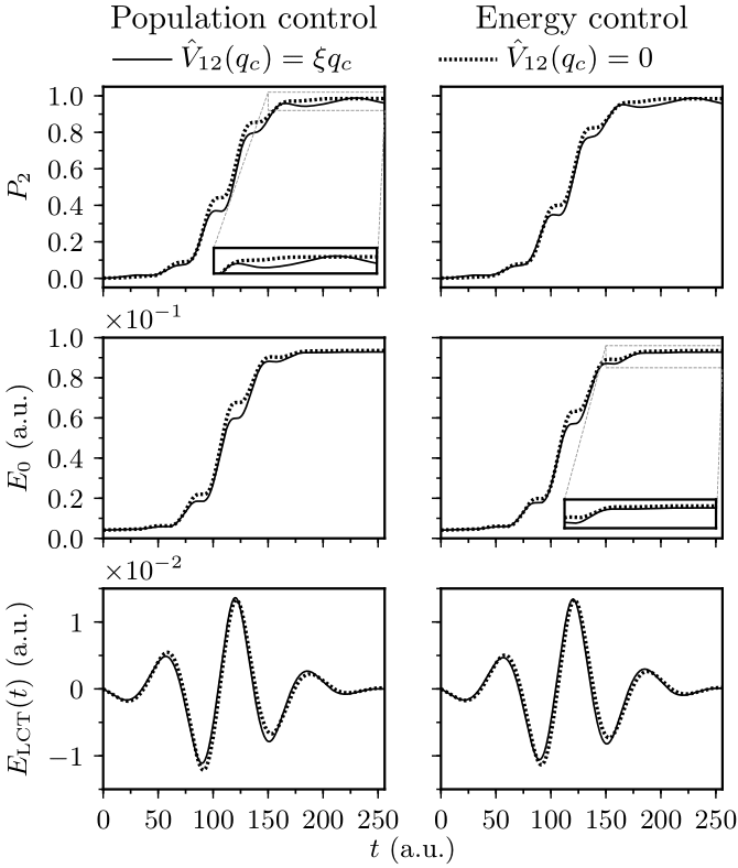
Figure 1: Local control calculations whose goal is increasing either the population $P_{2}:=\langle\mathbf{P}_{2}\rangle_{\psi_{t}}$ of the excited state (left panels, $\lambda=1.430\times 10^{-2}$) or the molecular energy $E_{0}(t):=\langle\mathbf{\hat{H}}_{0}\rangle_{\psi_{t}}$ (right panels, $\lambda=1.534\times 10^{-1}$). As expected, the local control theory applied to these closely related objectives yields very similar results. Top: Excited state population. Middle: Molecular energy. Bottom: Pulse obtained by local control theory.

Figure 1 shows the excited-state population, molecular energy, and obtained control pulse for the control of either the excited-state population (left panels) or molecular energy (right panels). In the figure, the results obtained in the presence and in the absence of nonadiabatic couplings are also compared for each target. The population and energy control schemes result in similar population dynamics and in both schemes, the population of the excited state reaches $0.99$ at time $t_{f}$. The carrier frequencies of the obtained control pulses are, as expected, similar and correspond to the electronic transition between the two electronic states of the model. As predicted, when controlling the excited-state population $\langle\mathbf{P}_{2}\rangle_{\psi_{t}}$ in the presence of nonadiabatic couplings given by Eq. (45), the evolution of the population is not monotonic (see the solid line in the inset of the top left panel of Fig. 1) because the control operator does not commute with the molecular Hamiltonian. Compare this with the monotonic increase of the population when the nonadiabatic couplings are zero [dotted line in the same inset; $\hat{V}_{12}(q_{c})=\hat{V}_{21}(q_{c})=0$] and the target operator commutes with the molecular Hamiltonian. In contrast, when controlling the molecular energy $\langle\hat{\mathbf{H}}_{0}\rangle_{\psi_{t}}$, its time evolution is always monotonic because the molecular Hamiltonian commutes with itself, whether the nonadiabatic couplings are included or not (see the inset of the middle right-hand panel of Fig. 1). Because increasing the population of the excited state has almost the same effect as increasing the molecular energy, very similar dynamics and control pulses are obtained. Yet, the energy and population controls do not always yield similar results. In the retinal model, when performing energy control, no vibrational energy is pumped into the system because the diagonal terms of the electric-dipole moment operator are all zero by construction (hence $\langle[\hat{\boldsymbol{\mu}},\hat{\mathbf{T}}]\rangle_{\psi_{t}}=0$). Consequently, only electronic potential energy is added to the system, and the corresponding control pulse is similar to the one obtained from the population control.

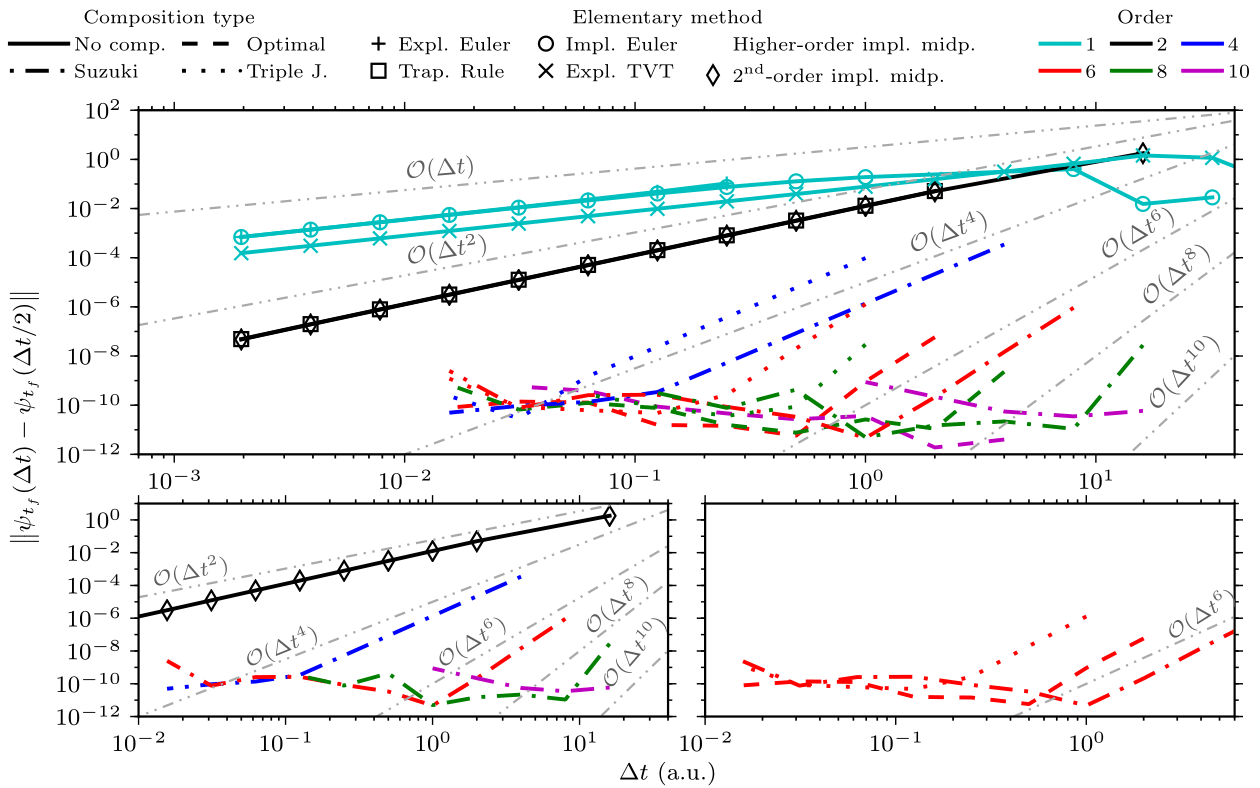
Figure 2: Convergence of the molecular wavefunction at the final time $t_{f}$ achieved by the local population control in the presence of nonadiabatic couplings. Top: All studied methods, i.e., explicit and implicit Euler methods, approximate explicit TVT split-operator algorithm, trapezoidal rule, implicit midpoint method and its symmetric compositions. Bottom-left: Methods obtained with the Suzuki composition. Bottom-right: Sixth-order methods obtained with different composition schemes.

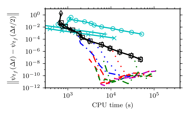
Figure 3: Efficiency of the integrators used for the local population control of retinal in the presence of nonadiabatic couplings. Efficiency is measured by plotting the convergence error as a function of the computational (CPU) cost. Line labels are the same as in Fig. 2.

To verify the orders of convergence predicted in Sec. III.2, we performed convergence analysis of control simulations using various integrators. Simulations with each integrator were repeated with different time steps and the resulting wavefunctions at the final time $t_{f}$ were compared. As a measure of the convergence error, we used the $L_{2}$-norm $\|\psi_{t_{f}}(\Delta t)-\psi_{t_{f}}(\Delta t/2)\|$, where $\psi_{t}(\Delta t)$ denotes the state at time $t$ obtained after propagation with time step $\Delta t$. Figure 2 displays the convergence behavior of both Euler methods, approximate explicit TVT split-operator algorithm, trapezoidal rule, and the proposed implicit midpoint method as well as its symmetric compositions, when controlling the excited state population. Notice that all integrators have their predicted orders of convergence. The approximate explicit TVT split-operator algorithm is, for the reasons mentioned in Sec. III.5, only first-order and not second-order as one might naïvely expect. For the convergence of other simulations, we refer the reader to Figs. S4-S6 of the supplementary material. Together, these results confirm that both population and energy control follow the predicted order of convergence regardless of the presence of nonadiabatic couplings.

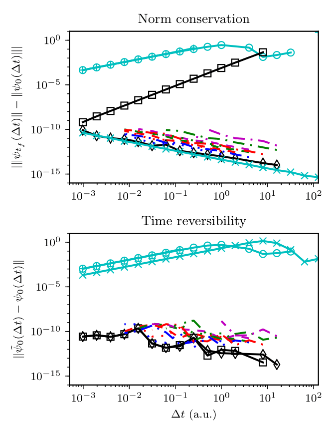
Figure 4: Norm conservation (left) and time reversibility (right) of various integrators at the final time $t_{f}$ as a function of the time step $\Delta t$ used for the local control of population in the presence of nonadiabatic couplings. Time reversibility is measured by the distance between the initial state $\psi_{0}$ and a “forward-backward” propagated state $\tilde{\psi}_{0}:=\hat{U}(0,t)\hat{U}(t,0)\psi_{0}$ [Eq. (11)] and line labels are the same as in Fig. 2.

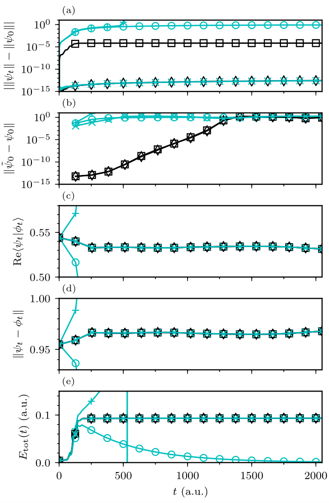
Figure 5: Geometric properties of various integrators used for the local population control in the presence of nonadiabatic couplings. Panel (a) shows that only the implicit midpoint and approximate explicit split-operator methods conserve the norm, while panel (b) demonstrates that only the implicit midpoint method and the trapezoidal rule are time-reversible. (Reversibility is measured as in Fig. 4). Bottom three panels show that no method conserves (c) the inner product, (d) distance between two states (which would imply stability), or (e) total energy $E_{\text{tot}}(t):=E_{0}(t)+\langle\hat{\mathbf{V}}_{\text{LCT}}(\psi_{t})\rangle_{\psi_{t}}$ because even the exact evolution operator does not preserve these properties. State $\phi_{0}$ is $\psi_{0}$ displaced along the reaction coordinate, i.e., a Gaussian wavepacket with parameters $q_{0}=(0.1,0)$, $p_{0}=(0,0)$, and $\sigma_{0}=(0.128,0)$ a.u. The time step $\Delta t=2^{-2}$ a.u. was used for all calculations and line labels are the same as in Fig. 2. Note that only a few points of the Euler methods are visible in some of the plots because the results of the Euler methods leave the range of these plots very rapidly.

Because the higher-order methods require more work to perform each step, a higher order of convergence may not guarantee higher efficiency. Therefore, we evaluated the efficiency of each method directly by measuring the computational cost needed to reach a prescribed convergence error. Figure 3 shows the convergence error as a function of the central processing unit (CPU) time and confirms that, except for very crude calculations, higher-order integrators are more efficient than any of the first- and second-order methods. For example, to reach errors below a rather high threshold of $3\times 10^{-4}$, the fourth-order integrator obtained with the Suzuki composition scheme is already more efficient than any of the first- or second-order algorithms. The efficiency gain increases further when highly accurate results are desired. Indeed, for an error of $10^{-9}$, the eighth-order optimal method is $48$ times faster than the basic, second-order implicit midpoint method and approximately $400000$ times faster than the approximate explicit TVT split-operator algorithm (for which, due to its inefficiency, the speedup had to be estimated by linear extrapolation). High accuracy is hard to achieve with the explicit methods because both the explicit Euler and approximate explicit TVT split-operator algorithms have only first-order convergence. Notice also that the cost of implicit methods is not a monotonous function of the error because the Newton-Raphson method needs more iterations to converge for larger than for smaller time steps. Indeed, for time steps (or errors) larger than a critical value, the CPU time might in fact increase with further increasing time step (or error). The efficiency plots of other control simulations (see Figs. S7-S9 of the supplementary material) confirm that the increase in efficiency persists regardless of the control target (energy or population) and presence or absence of nonadiabatic couplings.

Figure 4 analyzes how the time reversibility and norm conservation depend on the time step. The figure confirms that all proposed integrators are exactly time-reversible and norm-conserving regardless of the time step (the slow increase of the error with decreasing time step is due to the accumulation of numerical roundoff errors because a smaller time steps requires a larger number of steps to reach the same final time $t_{f}$). In contrast, the figure shows that an unrealistically small time step would be required for the trapezoidal rule and both Euler methods to conserve norm exactly and for the explicit split-operator algorithm to be exactly time-reversible. Figures S10-S12 of the supplementary material confirm that neither the chosen control objective nor the nonadiabatic couplings influence the geometric properties of the integrators.

We also checked how the conservation of geometric properties by the integrators depend on time $t$ for a fixed time step. For these simulations, we used a greater final time $t_{f}=2048$ a.u. and an intentionally large time step $\Delta t=2^{-2}$ a.u. The grid was modified to 256 points between $\theta=\pm 3\pi/2$ a.u. and 64 points between $q_{c}=\pm 9$ a.u., ensuring that the grid representation of the wavefunction at the final time $t_{f}$ was converged (see Fig. S2 of the supplementary material). Figure 5 displays the time evolution of the geometric properties for the elementary integrators (i.e., the trapezoidal rule, implicit midpoint, approximate explicit split-operator, and both Euler methods). The top panel confirms that the implicit midpoint method and the approximate explicit TVT split-operator algorithm conserve the norm exactly (i.e., to machine precision) even though a large time step was used. In contrast, the trapezoidal rule and both Euler methods do not conserve the norm. The second panel shows that only the trapezoidal rule and the implicit midpoint method are time-reversible. However, due to the nonlinearity of the Schrödinger equation (1) and the accumulation of roundoff errors, the time reversibility of these integrators slowly deteriorates as time increases. (For a more detailed analysis of this gradual loss of time reversibility, we refer the reader to Sec. V of the supplementary material.) The bottom three panels of Fig. 5 confirm that even the implicit midpoint method does not conserve the inner product, distance between two states, and total energy; this is not surprising because, due to nonlinearity, the exact solution does not conserve these properties either. Figures S13-S15 of the supplementary material also confirm that neither the chosen control objective nor the nonadiabatic couplings influence the time evolution of the geometric properties of these integrators.

V Conclusion

We presented high-order time-reversible integrators for the nonlinear time-dependent Schrödinger equation and demonstrated their efficiency and geometric properties on the problem of local control of quantum systems. The basic time-reversible integrator is an adaptation of the implicit midpoint method to the nonlinear Schrödinger equation and is obtained by composing the explicit and implicit Euler methods. It is norm-conserving, symmetric, time-reversible, and of second order of accuracy in the time step. Because it is symmetric, the implicit midpoint method can be composed using symmetric composition methods to obtain integrators of an arbitrary even order of accuracy. These higher-order integrators conserve all of the properties of the original second-order method.

In contrast, the explicit TVT split-operator algorithm is generally only an approximate adaptation of the standard second-order TVT split-operator algorithm to the nonlinear Schrödinger equation which results from LCT. Because this integrator is not implicit, it is only of first order accuracy in the time step and loses time reversibility while still conserving the norm. The trapezoidal rule, another popular algorithm for solving the Schrödinger equation, remains symmetric and time-reversible, but does not conserve the norm of the wavefunction propagated with a nonlinear Schrödinger equation.

Although we applied the proposed algorithms only to the special case of LCT, they should be useful for any nonlinear time-dependent Schrödinger equation if high accuracy, norm conservation, and time reversibility of the solution are desired.

The data that support the findings of this study are contained in the paper and supplementary material.

Supplementary material

See the supplementary material for a detailed description of the generalized minimal residual method, convergence of the wavefunction with respect to the grid density, a plot of the potential energy surfaces, an additional analysis of the convergence, efficiency, and geometric properties of various integrators, and a detailed analysis of the gradual loss of time reversibility of the implicit midpoint method.

Appendix A Geometric properties of various integrators

Here, we verify which geometric properties of the exact evolution are preserved by various integrators. The analysis generalizes the analysis from Appendix A of Ref. 36 for the linear to the nonlinear Schrödinger equation. To simplify the proofs, wherever it is not ambiguous, we shall use abbreviated notation $\hat{U}_{\text{appr}}(\psi):=\hat{U}_{\text{appr}}(t+\Delta t,t;\psi)$ for the evolution operator for a single time step and $\epsilon:=\Delta t/\hbar$ for the time step divided by Planck’s constant.

A.1 Norm conservation

In general, the norm is conserved if and only if

$$\hat{U}_{\text{appr}}(\psi)^{\dagger}\hat{U}_{\text{appr}}(\psi)=1,$$

which follows from a derivation analogous to Eq. (9) for the exact operator $\hat{U}(\psi)$. As in the linear case, neither Euler method conserves the norm because

$$\hat{U}_{\text{expl}}(\psi_{t})^{\dagger}\hat{U}_{\text{expl}}(\psi_{t}) =[1+i\epsilon\hat{H}(\psi_{t})][1-i\epsilon\hat{H}(\psi_{t})]$$

$$=1+\epsilon^{2}\hat{H}(\psi_{t})^{2}\neq 1$$ (46)

and

$$\hat{U}_{\text{impl}}(\psi_{t+\Delta t})^{\dagger}\hat{U}_{\text{impl}}(\psi_{t+\Delta t})$$

$$\qquad=[1-i\epsilon\hat{H}(\psi_{t+\Delta t})]^{-1}[1+i\epsilon\hat{H}(\psi_{t+\Delta t})]^{-1}$$

$$\qquad=[1+\epsilon^{2}\hat{H}(\psi_{t+\Delta t})^{2}]^{-1}\neq 1.$$ (47)

The trapezoidal rule, norm-conserving in the linear case, loses this property for nonlinear Hamiltonians since

$$\hat{U}_{\text{trap}}(\psi)^{\dagger}\hat{U}_{\text{trap}}(\psi)$$

$$\quad=[1+i\epsilon\hat{H}(\psi_{t})/2][1-i\epsilon\hat{H}(\psi_{t+\Delta t})/2]^{-1}$$

$$\qquad\times[1+i\epsilon\hat{H}(\psi_{t+\Delta t})/2]^{-1}[1-i\epsilon\hat{H}(\psi_{t})/2]$$

$$\quad=[1+i\epsilon\hat{H}(\psi_{t})/2][1+\epsilon^{2}\hat{H}(\psi_{t+\Delta t})^{2}/4]^{-1}$$

$$\qquad\times[1-i\epsilon\hat{H}(\psi_{t})/2]$$

$$\quad\neq 1;$$ (48)

the last nontrivial expression does not reduce to $1$ because $\hat{H}(\psi_{t})\neq\hat{H}(\psi_{t+\Delta t})$. In contrast, both the implicit midpoint and approximate explicit TVT split-operator algorithms conserve the norm even in the nonlinear setting because

$$\hat{U}_{\text{mid}}(\psi_{t+\Delta t/2})^{\dagger}\hat{U}_{\text{mid}}(\psi_{t+\Delta t/2})$$

$$\quad=[1-i\epsilon\hat{H}(\psi_{t+\Delta t/2})/2]^{-1}[1+i\epsilon\hat{H}(\psi_{t+\Delta t/2})/2]$$

$$\qquad\times[1-i\epsilon\hat{H}(\psi_{t+\Delta t/2})/2][1+i\epsilon\hat{H}(\psi_{t+\Delta t/2})/2]^{-1}$$

$$\quad=1$$ (49)

(where in the last step we used the commutativity of the middle two factors in the previous expression) and

$$\hat{U}_{\text{expl TVT}}({\psi_{t,\hat{T}\Delta t/2}})^{\dagger}\hat{U}_{\text{expl TVT}}({\psi_{t,\hat{T}\Delta t/2}})$$

$$\qquad=e^{i\epsilon\hat{T}/2}e^{i\epsilon\hat{V}_{\text{tot}}({\psi_{t,\hat{T}\Delta t/2}})}e^{i\epsilon\hat{T}/2}$$

$$\quad\qquad\times e^{-i\epsilon\hat{T}/2}e^{-i\epsilon\hat{V}_{\text{tot}}({\psi_{t,\hat{T}\Delta t/2}})}e^{-i\epsilon\hat{T}/2}$$

$$\qquad=1.$$ (50)

A.2 Symmetry and time reversibility

Neither Euler method is symmetric or time-reversible because they are adjoints of each other:

$$\hat{U}_{\text{expl}}(t+\Delta t,t;\psi_{t})^{\ast} =\hat{U}_{\text{expl}}(t,t+\Delta t;\psi_{t+\Delta t})^{-1}$$

$$=[1-i(-\Delta t)\hat{H}(\psi_{t+\Delta t})/\hbar]^{-1}$$

$$=\hat{U}_{\text{impl}}(t+\Delta t,t;\psi_{t+\Delta t}).$$ (51)

The approximate explicit TVT split-operator algorithm is also time-irreversible because forward propagation is not cancelled by backward propagation:

$$\hat{U}_{\text{expl TVT}}(t;t+\Delta t,\psi_{\hat{V}\hat{T}})\hat{U}_{\text{expl TVT}}(t+\Delta t;t,{\psi_{t,\hat{T}\Delta t/2}})$$

$$\qquad=e^{i\epsilon\hat{T}/2}e^{i\epsilon\hat{V}_{\text{tot}}(\psi_{\hat{V}\hat{T}})}e^{i\epsilon\hat{T}/2}$$

$$\quad\qquad\times e^{-i\epsilon\hat{T}/2}e^{-i\epsilon\hat{V}_{\text{tot}}({\psi_{t,\hat{T}\Delta t/2}})}e^{-i\epsilon\hat{T}/2}$$

$$\qquad\neq 1,$$ (52)

where ${\psi_{\hat{V}\hat{T}}:=e^{i\epsilon\hat{T}/2}\psi_{t+\Delta t}=e^{-i\epsilon\hat{V}_{\text{tot}}(\psi_{t,\hat{T}\Delta t/2})}}$$\psi_{t,\hat{T}\Delta t/2}$ denotes the state obtained after forward propagation of $\psi_{t,\hat{T}\Delta t/2}$ with the potential evolution operator and $\hat{V}_{\text{tot}}(\psi_{\hat{V}\hat{T}})\neq\hat{V}_{\text{tot}}(\psi_{t,\hat{T}\Delta t/2})$ was used to obtain the last line. It is clear from Eq. (52) that if the nonlinear term is as in the Gross-Pitaevskii equation, i.e., if $V_{\text{tot}}(\psi,q)=V_{0}(q)+C|\psi(q)|^{2}$ with $C$ a real constant, the approximate explicit TVT split-operator algorithm becomes time-reversible because $\hat{V}_{\text{tot}}(\psi_{\hat{V}\hat{T}})=\hat{V}_{\text{tot}}(\psi_{t,\hat{T}\Delta t/2})$ in that particular case; the reason is that wavefunctions $\psi_{\hat{V}\hat{T}}(q)$ and $\psi_{t,\hat{T}\Delta t/2}(q)$ in position representation only differ by a position-dependent phase factor. However, the equality $\hat{V}_{\text{tot}}(\psi_{\hat{V}\hat{T}})=\hat{V}_{\text{tot}}(\psi_{t,\hat{T}\Delta t/2})$ does not hold for other nonlinear Hamiltonians, such as the one in LCT, which contains a more general nonlinearity.

In contrast, both the implicit midpoint method and trapezoidal rule are always time-reversible because they are symmetric:

$$\hat{U}_{\text{mid}}(t+\Delta t,t;\psi_{t+\Delta t/2})^{\ast}=\hat{U}_{\text{mid}}(t,t+\Delta t;\psi_{t+\Delta t/2})^{-1}$$

$$\quad=\left([1+i\epsilon\hat{H}(\psi_{t+\Delta t/2})/2][1-i\epsilon\hat{H}(\psi_{t+\Delta t/2})/2]^{-1}\right)^{-1}$$

$$\quad=[1-i\epsilon\hat{H}(\psi_{t+\Delta t/2})/2][1+i\epsilon\hat{H}(\psi_{t+\Delta t/2})/2]^{-1}$$

$$\quad=\hat{U}_{\text{mid}}(t+\Delta t,t;\psi_{t+\Delta t/2}),$$ (53)

and

$$\hat{U}_{\text{trap}}(t+\Delta t,t;\psi)^{\ast}=\hat{U}_{\text{trap}}(t,t+\Delta t;\psi)^{-1}$$

$$\quad=\left([1-i\epsilon\hat{H}(\psi_{t})/2]^{-1}[1+i\epsilon\hat{H}(\psi_{t+\Delta t})/2]\right)^{-1}$$

$$\quad=[1+i\epsilon\hat{H}(\psi_{t+\Delta t})]^{-1}[1-i\epsilon\hat{H}(\psi_{t})/2]$$

$$\quad=\hat{U}_{\text{trap}}(t+\Delta t,t;\psi).$$ (54)

References

- Frenkel [1934] J. Frenkel, Wave mechanics (Clarendon Press, Oxford, 1934).
- Dirac [1930] P. A. M. Dirac, Math. Proc. Cambridge Philos. 26, 376–385 (1930).
- Broeckhove et al. [1988] J. Broeckhove, L. Lathouwers, E. Kesteloot, and P. V. Leuven, Chem. Phys. Lett. 149, 547 (1988).
- Lubich [2008] C. Lubich, From Quantum to Classical Molecular Dynamics: Reduced Models and Numerical Analysis, 12th ed. (European Mathematical Society, Zürich, 2008).
- Meyer, Manthe, and Cederbaum [1990] H.-D. Meyer, U. Manthe, and L. S. Cederbaum, Chem. Phys. Lett. 165, 73 (1990).
- Manthe, Meyer, and Cederbaum [1992] U. Manthe, H. Meyer, and L. S. Cederbaum, J. Chem. Phys. 97, 3199 (1992).
- Beck et al. [2000] M. Beck, A. Jäckle, G. Worth, and H.-D. Meyer, Phys. Rep. 324, 1 (2000).
- Lanczos [1950] C. Lanczos, J. Res. Nat. Bur. Stand. 45, 255 (1950).
- Leforestier et al. [1991] C. Leforestier, R. H. Bisseling, C. Cerjan, M. D. Feit, R. Friesner, A. Guldberg, A. Hammerich, G. Jolicard, W. Karrlein, H.-D. Meyer, N. Lipkin, O. Roncero, and R. Kosloff, J. Comp. Phys. 94, 59 (1991).
- Park and Light [1986] T. J. Park and J. C. Light, J. Chem. Phys. 85, 5870 (1986).
- Anderson et al. [1995] M. H. Anderson, J. R. Ensher, M. R. Matthews, C. E. Wieman, and E. A. Cornell, Science 269, 198 (1995).
- Dalfovo et al. [1999] F. Dalfovo, S. Giorgini, L. P. Pitaevskii, and S. Stringari, Rev. Mod. Phys. 71, 463 (1999).
- Gross [1961] E. P. Gross, Il Nuovo Cimento (1955-1965) 20, 454–477 (1961).
- Pitaevskii [1961] L. P. Pitaevskii, Sov. Phys. JETP 13 (1961).
- Carles [2002] R. Carles, Ann. Henri Poincaré 3, 757 (2002).
- Carles, Markowich, and Sparber [2008] R. Carles, P. A. Markowich, and C. Sparber, Nonlinearity 21, 2569 (2008).
- Minguzzi et al. [2004] A. Minguzzi, S. Succi, F. Toschi, M. Tosi, and P. Vignolo, Phys. Rep. 395, 223 (2004).
- Bao, Jaksch, and Markowich [2003] W. Bao, D. Jaksch, and P. A. Markowich, J. Comp. Phys. 187, 318 (2003).
- Chang, Jia, and Sun [1999] Q. Chang, E. Jia, and W. Sun, J. Comp. Phys. 148, 397 (1999).
- Antoine, Bao, and Besse [2013] X. Antoine, W. Bao, and C. Besse, Comp. Phys. Comm. 184, 2621 (2013).
- Feit, Fleck, and Steiger [1982] M. D. Feit, J. A. Fleck, Jr., and A. Steiger, J. Comp. Phys. 47, 412 (1982).
- Kosloff and Kosloff [1983a] D. Kosloff and R. Kosloff, J. Comp. Phys. 52, 35 (1983a).
- Kosloff and Kosloff [1983b] R. Kosloff and D. Kosloff, J. Chem. Phys. 79, 1823 (1983b).
- Tannor [2007] D. J. Tannor, Introduction to Quantum Mechanics: A Time-Dependent Perspective (University Science Books, Sausalito, 2007).
- Kosloff et al. [1989] R. Kosloff, S. A. Rice, P. Gaspard, S. Tersigni, and D. J. Tannor, Chem. Phys. 139, 201 (1989).
- Kosloff, Hammerich, and Tannor [1992] R. Kosloff, A. D. Hammerich, and D. Tannor, Phys. Rev. Lett. 69, 2172 (1992).
- Marquetand et al. [2006] P. Marquetand, S. Gräfe, D. Scheidel, and V. Engel, J. Chem. Phys. 124, 054325 (2006).
- Engel, Meier, and Tannor [2009] V. Engel, C. Meier, and D. J. Tannor, Adv. Chem. Phys. 141 (2009).
- Marquetand and Engel [2006] P. Marquetand and V. Engel, Chem. Phys. Lett. 426, 263 (2006).
- Marquetand and Engel [2007] P. Marquetand and V. Engel, J. Chem. Phys. 127, 084115 (2007).
- Bomble et al. [2011] L. Bomble, A. Chenel, C. Meier, and M. Desouter-Lecomte, J. Chem. Phys. 134, 204112 (2011).
- Vranckx et al. [2015] S. Vranckx, J. Loreau, N. Vaeck, C. Meier, and M. Desouter-Lecomte, J. Chem. Phys. 143, 164309 (2015).
- Yamaki et al. [2005] M. Yamaki, K. Hoki, Y. Ohtsuki, H. Kono, and Y. Fujimura, J. Am. Chem. Soc. 127, 7300 (2005).
- Vindel-Zandbergen, Meier, and Sola [2016] P. Vindel-Zandbergen, C. Meier, and I. R. Sola, Chem. Phys. 478, 97 (2016).
- Roulet, Choi, and Vaníček [2019] J. Roulet, S. Choi, and J. Vaníček, J. Chem. Phys. 150, 204113 (2019).
- Choi and Vaníček [2019] S. Choi and J. Vaníček, J. Chem. Phys. 150, 204112 (2019).
- Hahn and Stock [2000] S. Hahn and G. Stock, J. Phys. Chem. B 104, 1146 (2000).
- Lasser and Lubich [2020] C. Lasser and C. Lubich, “Computing quantum dynamics in the semiclassical regime,” (2020), arXiv:2002.00624 [math.NA] .
- Schatz and Ratner [2002] G. C. Schatz and M. A. Ratner, Quantum Mechanics in Chemistry (Dover Publications, 2002).
- Halmos [1942] P. R. Halmos, Finite dimensional vector spaces (Princeton University Press, 1942).
- Leimkuhler and Reich [2004] B. Leimkuhler and S. Reich, Simulating Hamiltonian Dynamics (Cambridge University Press, 2004).
- Hairer, Lubich, and Wanner [2006] E. Hairer, C. Lubich, and G. Wanner, Geometric Numerical Integration: Structure-Preserving Algorithms for Ordinary Differential Equations (Springer Berlin Heidelberg New York, 2006).
- Yoshida [1990] H. Yoshida, Phys. Lett. A 150, 262 (1990).
- Suzuki [1990] M. Suzuki, Phys. Lett. A 146, 319 (1990).
- Kahan and Li [1997] W. Kahan and R.-C. Li, Math. Comput. 66, 1089 (1997).
- Sofroniou and Spaletta [2005] M. Sofroniou and G. Spaletta, Optim. Method Softw. 20, 597 (2005).
- Press et al. [1992] W. H. Press, S. A. Teukolsky, W. T. Vetterling, and B. P. Flannery, Numerical recipes in C (Cambridge University Press, Cambridge, UK, 1992).
- Saad and Schultz [1986] Y. Saad and M. H. Schultz, SIAM J. Sci. Stat. Comp. 7, 856 (1986).
- Saad [2003] Y. Saad, Iterative Methods for Sparse Linear Systems, 2nd ed. (SIAM, 2003).
- Arnoldi [1951] W. E. Arnoldi, Quart. Appl. Math. 9, 17 (1951).
- Saad [1980] Y. Saad, Linear Algebra Appl. 34, 269 (1980).
- Petersen and Pedersen [2012] K. B. Petersen and M. S. Pedersen, “The matrix cookbook,” (2012).
- Frigo and Johnson [2005] M. Frigo and S. G. Johnson, Proc. IEEE 93, 216 (2005).