Primary Control Effort under Fluctuating Power Generation in Realistic High-Voltage Power Networks
Abstract
Many recent works in control of electric power systems have investigated their synchronization through global performance metrics under external disturbances. The approach is motivated by fundamental changes in the operation of power grids, in particular by the substitution of conventional power plants with new renewable sources of electrical energy. This substitution will simultaneously increase fluctuations in power generation and reduce the available mechanical inertia. It is crucial to understand how strongly these two evolutions will impact grid stability. With very few, mostly numerical exceptions, earlier works on performance metrics had to rely on unrealistic assumptions of grid homogeneity. Here we show that a modified spectral decomposition can tackle that issue in inhomogeneous power grids in cases where disturbances occur on time scales that are long compared to the intrinsic time scales of the grid. We find in particular that the magnitude of the transient excursion generated by disturbances with long characteristic times does not depend on inertia. For continental-size, high-voltage power grids, this corresponds to power fluctuations that are correlated on time scales of few seconds or more. We conclude that power fluctuations arising from new renewables will not require per se the deployment of additional rotational inertia. We numerically illustrate our results on the IEEE 118-Bus test case and a model of the synchronous grid of continental Europe.
Index Terms:
Low inertia power systems, high-voltage transmission grids, transient stability, performance metrics.I Introduction
The penetration of new renewable sources of electrical energy is currently increasing in most electric power grids worldwide, as more and more traditional power plants are phased out. A major concern is obviously that this substitution reduces the available inertia while it simultaneously induces larger fluctuations in power generation [1]. Both changes may jeopardize grid stability, either individually or taken together. A key issue is accordingly to evaluate how much power grids need to be adapted to their resulting new modes of operation – for instance through line extensions or deployment of resources providing ancillary services [2]. To ensure the stability of the grid and the safety of power supply, it is important to clarify the role of the generators dynamical parameters that will be affected by this transition, namely the rotational inertia and the frequency damping / droop control. Both are going to be globally reduced, moreover their geographical distribution will be modified. To try to identify which of these dynamical parameters are most crucial, where they should be primarily deployed, as well as when and in what operating conditions they are most needed, analytical and numerical works have investigated the robustness of electric power grids under external disturbances. The response of power grids to external disturbances has been investigated through quadratic performance metrics [3, 4, 5, 6, 7, 8, 9, 10, 11, 12], eigenvalue damping ratios and frequency overshoots [13], rate of change of frequency[8, 14] or disturbance wave propagation [15, 16]. Except for numerical results [13, 15, 16], these works considered disturbances with infinitely short time scales, such as white noise power fluctuations or instantaneous power injection changes [3, 5, 6, 7, 9, 10, 11, 12], or with infinitely long time scales, such as step changes in power injection [8, 14]. All of the analytical works relied on one of the two homogeneity assumptions that inertia and frequency damping are the same everywhere, or that their ratio is.
These homogeneity assumptions are not representative of real power grids, where in particular, consumer nodes are inertialess but with small, albeit finite frequency damping [17, 18]. Often, this inconsistency is circumvented by invoking a prior Kron reduction absorbing the inertialess nodes into an effective network. One then measures the robustness of that reduced network, which may or may not be related to the robustness of the original one, because Kron reduction does not capture the dynamics of the reduced, inertialess nodes. To the best of our knowledge, Ref. [11] is the first work that tolerates deviations from homogeneity in an analytical calculation of a quadratic performance metric. Its results suggest that grid robustness is crucially sensitive to the geographic distribution of frequency control, while inertia has to be distributed rather evenly. This conclusion has to be revisited because, first, Ref. [11] is based on an approximate method tolerating only small deviations from homogeneity and second, the only disturbances it considers are long power losses.
In this manuscript, we investigate the response of power systems to colored noisy power fluctuations. We quantify the response to these disturbances by a quadratic performance metric measuring the primary control effort necessary to absorb the fault [7]. Our analytical approach still relies on a homogeneity assumption. Our results however emphasize the role played by the different time scales in the problem: the performance metric depends on inertia only when the characteristic time scale of the disturbance is long compared to all other time scales in the system. In that case we conjecture, and confirm numerically, that our analytical results also apply to heterogeneous systems. In continental-size high-voltage power grids, the network time scales are shorter than few seconds [19]. Therefore, noise fluctuating on time scales of tens of second or more induces transients whose amplitude, duration and oscillations are largely independent of inertia, and our analytical results directly apply to most disturbances on realistic, inhomogeneous high voltage power grids.
The manuscript is organized as follows. Section II defines our mathematical notations. Section III defines the power network model and gives an analytical expression for its linear response. Section IV introduces performance metrics and gives analytical expressions for them. Of particular interest are the short- and long-correlation time asymptotics. In Sec. V, we numerically confirm our theory on both the IEEE 118-Bus test case and the PanTaGruEl model of the synchronous grid of continental Europe. We discuss time scales in such high-voltage power grids and show that the corresponding performance metric is given by the long noise correlation time asymptotic limit. Our conclusions are given in section VI.
II Mathematical Notation
Given a vector , we denote its transpose by . We write for the diagonal matrix with on its diagonal. The -th unit vector with a single nonzero component is . The scalar product of two vectors is written and the scalar product of a vector with itself is . The statistical average of a random variable is . Finally, considering a diagonal matrix , we denote its power as .
III Power Grids and their Response to Fluctuating Power Injections
III-A Swing dynamics near synchrony
Transient dynamics in high-voltage power networks is commonly modelled by the swing equations which describe the dynamics of voltage angles assuming constant voltage amplitudes. In the lossless line approximation, appropriate to very high-voltages [18], they read
| (1) |
where each network node is labeled with a voltage angle . Equation (1) is written in a rotating frame, so that the frequency refers to the deviation from the rated frequency of or Hz. Each node has inertia and damping control parameters and respectively, and an active power that is generated () or consumed (). The coupling between node and is given by the susceptance of the corresponding power line. The operational state is a synchronous stationary solution to Eq. (1).
Equation (1) is governed by two sets of time scales. The first set is given by the ratio between inertia and damping coefficients . It corresponds to the local relaxation of synchronous machines. The second one is determined by the network characteristic time scales given by damping coefficients and the eigenvalues of the weighted Laplacian, see Eq. (3) below. Depending on these two sets of time scales, perturbations are locally damped or spread across the network. In a synthetic synchronous grid of continental Europe with constant damping and inertia corresponding to the average of their true values, it has been found that all modes are underdamped and propagate through the whole system with , [19].
We next investigate the response of the system to a time-dependent disturbance acting on the operational state , following which angles become time-dependent, . The small-signal response is governed by dynamical equations obtained after linearizing Eq. (1) about ,
| (2) |
where we introduced inertia and damping matrices, and and the weighted Laplacian matrix with matrix elements
| (3) |
This Laplacian is minus the stability matrix of the linearized dynamics, and since we consider a stable synchronous state, it is positive semidefinite, with a single vanishing eigenvalue with eigenvector . All other eigenvalues are positive, , . Equation (2) can be integrated via a spectral decomposition provided either: (i) both and commute with , then Eq. (2) can be integrated in the eigenspace of , or (ii) , in which case Eq. (2) can be integrated in the eigenspace of .
III-B Analytical solution for constant damping-to-inertia ratio
We consider the case (ii) above of constant inertia-to-damping ratio, . To calculate the response of the system, we first perform a change of variable on Eq. (2). We obtain
| (4) |
We choose this normalization with , rather than with as proposed in Ref. [8], because it allows us to treat the inertialess case with , from which we will extrapolate the realistic case where consumer nodes are inertialess and generator nodes have nonhomogeneous inertia. Equation (4) can be solved by expanding angle deviations as , over the eigenvectors of . The matrix is no longer Laplacian but it still has a zero-mode . Angle shifts of along do not modify the synchronous state because . Note also that, by orthogonality with , eigenvector components must satisfy for .
Proposition III.1
The general solution to Eq. (4) reads
| (5) | ||||
with where is the eigenvalue associated with the eigenvector of .
Proof:
We first expand angle deviations over the eigenbasis of as . From the orthogonality of the eigenbasis, , one straightforwardly rewrites Eq. (4) as
| (6) |
for . The expansion coefficients can be read from Eq. (5), and direct differentiation shows that they solve this equation. This completes the proof. ∎
IV Dynamical Parameters and Transient Excursions
IV-A Quantifying frequency excursions
To evaluate the global response of the system to an external disturbance, we use the following performance metric
| (7) | ||||
because it measures the primary control effort and therefore has a physical meaning [7]. The quantity with gives the average frequency deviation over all nodes in the system. Because synchronous states are defined modulo any homogeneous angle shift, the transformation does not change the synchronous state. Accordingly only phase and frequency shifts with and matter. This is included in by subtracting the average . That is a performance metric is easily understood: low values indicate that the system absorbs the perturbation with little fluctuations, while large values indicate a large transient excursion around the initial synchronous state. Using the above change of variables, , Eq. (7) becomes,
| (8) | ||||
This can be calculated using the explicit expression for from Eq. (5), once a perturbation is given.
Proposition IV.1
Consider a noisy disturbance acting on of the network nodes. The noise ensemble is Gaussian and defined by its vanishing first moments, , and its second moments with the noise correlation time . The performance metric for primary control effort averaged over this noise ensemble is given by
| (9) | ||||
Corollary 1
In the limit of short noise correlation time, one has
| (10) | ||||
Corollary 2
In the opposite asymptotic limit, one has
| (11) | ||||
Proof:
Inserting the time derivative of Eq. (5) into Eq. (8) and taking the average over the noise ensemble
with
gives Eq. (9), with few straightforwardly calculated exponential integrals. The two asymptotic results (10) and (11)
are easily obtained by a Taylor expansion, keeping only the first non-vanishing term. To obtain Eq. (10),
we also used .
∎
Remark 1: The short correlation time asymptotic of Eq. (10) agrees with the result of [7] obtained for either single-pulsed or averaged white-noise perturbations.
Remark 2: The noise correlators are defined either as time averages, or as averages over different noise sequences.
Proposition IV.2
Under the same assumptions as Proposition IV.1, the variance of the performance metric for primary control effort over the noise ensemble vanishes as as .
The proof proceeds through direct calculation of . It is too long to fit in this article and here we only sketch it. From Eq. (8) one has
| (12) | ||||
From Eq. (5), each contains a noise term . The noise average in the first term on the right-hand side of Eq. (12) therefore consists in pairings of four noise terms. There are three such contributions. The first one pairs the two ’s in and the two ’s in . This contribution is cancelled by a similar pairing in . The other two contributions pair ’s across indices and and accordingly, they constrain the values that and can take with respect to one another, . Accordingly, the double time integral in Eq. (12) gives a contribution , instead of , resulting in .
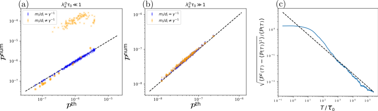
Remark 4: Proposition IV.2 means that for specific noisy disturbances satisfying the assumption of Proposition IV.1 and for long enough observation times , . The statistical average is therefore representative of specific noise disturbances for sufficiently long observation time. The validity of Proposition IV.2 is illustrated numerically in Fig. 1 (c).
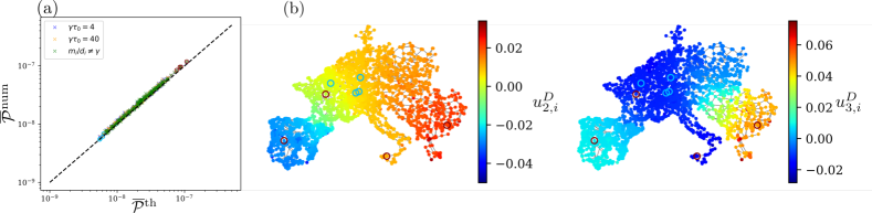
The two asymptotic limits of large and small are particularly interesting as they shed light on the influence of dynamical parameters, in particular on the interplay between local disturbance absorption by inertia and long-range propagation through low-lying network modes. First, in the short correlation time limit given by Eq. (10), explicitly depends on inertia but not on the coupling network. This reflects the fact that, in the white-noise limit, the perturbation remains local and is easily absorbed, if there is enough inertia. Second, Eq. (11) shows that, in the long correlation time limit, does not depend on inertia. This suggests that changing inertia in any direction will not change in the limit of long noise correlation time. This is a conjecture since Eq. (11) has been derived under the assumption of constant damping-to-inertia ratio, . Below we numerically confirm this conjecture. Simultaneously, Eq. (11) also shows that, in the long correlation time limit, is determined by the structure of the coupling network, with the modes with smallest eigenvalues having the largest influence. Those modes are extended over the whole network in large power grids, as is illustrated in Fig. 2 (b). Accordingly, in the limit of long noise correlation time, the disturbance is able to propagate over large distances in the network, and inertia has little influence on this large-scale propagation.
Remark 5: It is important to realize that fluctuations of renewable energy sources occur on time scales that are large compared to the intrinsic time scales of the power system [20]. As a matter of fact, time scales in the synchronous grid of continental Europe have been found to satisfy and [19]. Provided the above conjecture is corroborated, Eqs. (9)–(11) suggest that fluctuations from new renewables excite network modes and are efficiently absorbed by optimizing the distribution of damping with little regard for inertia. This conjecture is numerically confirmed below.
Remark 6: Similar conclusions as in Eqs. (9)–(11) regarding local inertia absorption vs. large-scale mode propagation are obtained in the case of step disturbances corresponding to sudden power losses, as a function of their duration .
Remark 7: The lossless line approximation used in this paper does not account for ohmic dissipation. We expect that the latter enhances mode damping and accordingly undermines disturbance propagation in the case of noise with long correlation time, but that it affects only marginally our result for short correlation time. Investigations beyond the lossless line approximation would be very welcome but lie beyond the scope of the present paper.
V Numerical Simulations
V-A Dynamical parameters for simulations
We consider two different cases: (i) cases with homogeneous damping-to-inertia ratio ; (ii) realistic heterogeneous cases, using the nonlinear swing dynamics of Eq. (1). In the homogeneous case, we used , where is the produced/consumed power at nominal frequency , and set . In the heterogeneous case, the inertia parameter vanishes on consumer nodes and is on generator nodes, where depends on the type of generator [18]. Damping is given by Eq. (5.24) and Table 4.3 in Ref. [18] for generators and by for consumer nodes. In all cases we use . For the IEEE-118 Bus test case discussed in Section V-B, and . For the PanTaGruEl European model discussed in Section V-D), and varies according to the generator type as described in Ref. [21].
V-B IEEE 118-Bus test case
The main prediction from Eqs. (9)-(11) is that, for noise correlation that is longer than the other characteristic time scales in the system, the performance metric does not depend on inertia parameters. This was conjectured from Eq. (11) where inertia does not appear. Fig. 1 shows performance metric obtained from individual noisy disturbance of a single node, repeating the operation for all nodes in the IEEE 118-Bus test case. As disturbance, we take Gaussian noise with the same first two moments as in Proposition IV.1. First, the primary control effort is calculated for a constant damping-to-inertia ratio (blue crosses), then for a distribution of dynamical parameters where generator nodes have inertia while consumer nodes do not (orange squares and crosses). As predicted by Eq. (11), for long correlation time of the noise [panel (b), ], the two distributions of dynamical parameters give the same , corroborating our conjecture that it does not depend on inertia. We have found (but do not show) that the performance metric only depends on the damping distribution in that case.
For short noise correlation time, on the other hand, Eq. (10) explicitly depends on the damping-to-inertia ratio , and we expect that the numerical data will differ from the theoretical prediction once this ratio is no longer constant. This is confirmed in Fig. 1 [panel (a), ] where with , numerical data fall on the theory (blue crosses). However, once is no longer constant, numerical data and theoretical prediction differ significantly (orange symbols). Quite interestingly, we found that for noisy perturbations on generator nodes with inertia, the theory still gives a remarkably accurate estimate for the primary control effort . An understanding of this remarkable agreement would be highly welcome, particularly since it could justify dynamic performance analysis on Kron reduced networks.
V-C Time scales in high-voltage electric power grids
We have shown that the primary control effort against fluctuating disturbances in the form of colored noise behaves very differently depending on the position of the noise correlation time relative to the characteristic time scales in the system. Furthermore the primary control effort is captured by our theory even for inhomogeneous dynamical parameters, when the noise correlation time is long enough. It is therefore desirable to identify what regime applies to a realistic high-voltage power grid subjected to fluctuating sources of power, in particular those generated by new renewable sources of energy. To that end, we consider in the next paragraph a realistic model of the synchronous grid of continental Europe [19, 21], with the following time scales
| (13a) | ||||
| (13b) | ||||
where means that we take the average over all nodes in the grid. It is commonly accepted that power fluctuations from renewable energy sources such as wind turbines or photovoltaic panels fluctuate on time scales that are larger than both time scales in Eq. (13) [20]. Therefore, the asymptotic limit of large noise correlation time, corresponding to Eq. (11) applies, and we expect that the primary control effort as measured by Eq. (7) is influenced only by damping, and not by inertia. Numerical results to be presented in the next paragraph corroborate this expectation.
As a side-remark we note that when the perturbation corresponds to the sudden disconnection of a power generator, controls usually try to reconnect the bus several times quickly after the fault (typically within few AC cycles). The typical time scale for such a perturbation is then less than several if not all system’s time scales, and inertia obviously matters to absorb such sudden faults, as it is predicted by Eq. (10).
V-D The PanTaGruEl European model
To further illustrate the influence of dynamical parameters on the primary control effort, we numerically compute Eq. (7) on the large-scale PanTaGruEl model of the European high-voltage transmission grid [21]. The model is shown on Fig. 2 (b). It has 3809 nodes and 4944 lines. More details can be found in Ref. [21]. We considered three different cases, (i) a homogeneous situation that corresponds to today’s grid in terms of its global amount of inertia, with and constant, (ii) a homogeneous situation where the inertia is reduced by a factor , i.e. , and constant, and (iii) a realistic situation with inhomogeneous damping parameters and where inertia vanishes on consumer nodes and is inhomogeneous on production nodes as described in Section V-A and Ref. [21], with larger than all other time scales in the system. Remarkably, Fig. 2 (a) shows that the primary control effort for all cases is well predicted by Eq. (11). This confirms our main finding that, for fluctuations with a correlation time longer than any other characteristic time scale in the system, inertia does not affect the primary control effort, Eq. (11). Quite surprisingly, an overall reduction of the total available inertia by a factor of 10 does not affect the primary control effort, Eq. (7).
VI Conclusion
With the ongoing energy transition resulting in strongly increased penetrations of new renewable sources of electrical energy, a question of crucial importance is how grid stability will evolve, given the resulting reduction of globally available rotational inertia and enhanced power fluctuations. We have shown that reduced inertia may pose problems only for perturbation occurring/fluctuating on very short time scales, shorter than all other characteristic time scales in the system. In continental-size transmission grids, these time scales are shorter than few seconds, consequently, power fluctuations from new renewables will not affect grid stability per se.
Inertia is of course important to absorb sudden faults occurring on very short time scales such as line faults or disconnection/reconnection of large power plants and so forth. Simultaneously, our result of Eq. (10) indicates that the resulting primary control effort is independent of the grid topology. Accordingly, optimal inertia distribution needs to follow the distribution of potential faults, for instance being larger in regions with higher density of generators. A similar conclusion was drawn in Refs. [7] and [11].
References
- [1] A. Ulbig, T. S. Borsche, and G. Andersson, “Impact of low rotational inertia on power system stability and operation,” IFAC Proceedings Volumes, vol. 47, no. 3, pp. 7290–7297, 2014.
- [2] “Power systems of the future: The case for energy storage, distributed generation, and microgrids,” Tech. Rep., IEEE Smart Grid, Tech. Rep. Nov. 2012.
- [3] B. Bamieh and D. F. Gayme, “The price of synchrony: Resistive losses due to phase synchronization in power networks,” American Control Conference, pp. 5815–5820, June 2013.
- [4] F. Dörfler, M. Jovanovic, M. Chertkov, and F. Bullo, “Sparsity-promoting optimal wide-area control of power networks,” IEEE Trans. Power Syst., vol. 29, no. 5, pp. 2281–2291, 2014.
- [5] E. Tegling, B. Bamieh, and D. F. Gayme, “The price of synchrony: Evaluating the resistive losses in synchronizing power networks,” IEEE Trans. Control Net. Syst., vol. 2, no. 3, pp. 254–266, 2015.
- [6] M. Siami and N. Motee, “Fundamental limits and tradeoffs on disturbance propagation in linear dynamical networks,” IEEE Transactions on Automatic Control, vol. 61, no. 12, pp. 4055–4062, Dec 2016.
- [7] B. K. Poolla, S. Bolognani, and F. Dörfler, “Optimal Placement of Virtual Inertia in Power Grids,” IEEE Transaction Automatic Control, vol. 62, no. 12, pp. 6209–6220, 2017.
- [8] F. Paganini and E. Mallada, “Global performance metrics for synchronization of heterogeneously rated power systems: The role of machine models and inertia,” 55th Annual Allerton Conference on Communication, Control, and Computing, pp. 324–331, 2017.
- [9] T. W. Grunberg and D. F. Gayme, “Performance measures for linear oscillator networks over arbitrary graphs,” IEEE Transactions on Control of Network Systems, vol. 5, no. 1, pp. 456–468, March 2018.
- [10] T. Coletta and P. Jacquod, “Performance measures in electric power networks under line contingencies,” IEEE Transactions on Control of Network Systems, vol. 7, pp. 221–231, 2020.
- [11] L. Pagnier and P. Jacquod, “Optimal placement of inertia and primary control: A matrix perturbation theory approach,” IEEE Access, vol. 7, pp. 145 889–145 900, 2019.
- [12] Y. Jiang, R. Pates, and E. Mallada, “Dynamic droop control in low-inertia power systems,” 2019.
- [13] A. Mešanović, U. Münz, and C. Heyde, “Comparison of , , and pole optimization for power system oscillation damping with remote renewable generation,” IFAC-PapersOnLine, vol. 49, no. 27, pp. 103–108, 2016.
- [14] L. Guo, C. Zhao, and S. H. Low, “Graph laplacian spectrum and primary frequency regulation,” IEEE Conference on Decision and Control, pp. 158–165, 2018.
- [15] S. Tamrakar, M. Conrath, and S. Kettemann, “Propagation of disturbances in ac electricity grids,” Scientific reports, vol. 8, no. 1, p. 6459, 2018.
- [16] H. Haehne, K. Schmietendorf, S. Tamrakar, J. Peinke, and S. Kettemann, “Propagation of wind-power-induced fluctuations in power grids,” Phys. Rev. E, vol. 99, no. 5, p. 050301, 2019.
- [17] A. R. Bergen and D. J. Hill, “A structure preserving model for power system stability analysis,” IEEE Transaction on Power Appartus and Systems, vol. PAS-100, p. 25, 1981.
- [18] J. Machowski, J. W. Bialek, and J. R. Bumby, Power System Dynamics, 2nd ed. Chichester, U.K: Wiley, 2008.
- [19] M. Tyloo, L. Pagnier, and P. Jacquod, “The key player problem in complex oscillator networks and electric power grids: Resistance centralities identify local vulnerabilities,” Science Advances, vol. 5, no. 11, 2019.
- [20] A. von Meier, “Integration of renewable generation in california: Coordination challenges in time and space,” in 11th International Conference on Electrical Power Quality and Utilisation, Oct 2011, pp. 1–6.
- [21] L. Pagnier and P. Jacquod, “PanTaGruEl - a pan-European transmission grid and electricity generation model,” Dec. 2019. [Online]. Available: https://doi.org/10.5281/zenodo.2642175