Ginkgo: A Modern Linear Operator Algebra Framework for High Performance Computing

Abstract.

In this paper, we present Ginkgo, a modern C++ math library for scientific high performance computing. While classical linear algebra libraries act on matrix and vector objects, Ginkgo’s design principle abstracts all functionality as “linear operators,” motivating the notation of a “linear operator algebra library.” Ginkgo’s current focus is oriented towards providing sparse linear algebra functionality for high performance GPU architectures, but given the library design, this focus can be easily extended to accommodate other algorithms and hardware architectures. We introduce this sophisticated software architecture that separates core algorithms from architecture-specific backends and provide details on extensibility and sustainability measures. We also demonstrate Ginkgo’s usability by providing examples on how to use its functionality inside the MFEM and deal.ii finite element ecosystems. Finally, we offer a practical demonstration of Ginkgo’s high performance on state-of-the-art GPU architectures.

1. Introduction

With the rise of manycore accelerators, such as graphics processing units (GPUs), there is an increasing demand for linear algebra libraries that can efficiently transform the massive hardware concurrency available in a single compute node into high arithmetic performance. At the same time, more and more application projects adopt object-oriented software designs based on C++.

In this paper, we present the result from our effort toward the design and development of Ginkgo, a next-generation, high performance sparse linear algebra library for multicore and manycore architectures. The library combines ecosystem extensibility with heavy, architecture-specific kernel optimization using the platform-native languages CUDA (for NVIDIA GPUs), HIP (for AMD GPUs), and OpenMP (for general-purpose multicore processors, such as those from Intel, AMD or ARM). The software development cycle that drives Ginkgo ensures production-quality code by featuring unit testing, automated configuration and installation, Doxygen code documentation, as well as a continuous integration and continuous benchmarking framework. Ginkgo is an open source effort licensed under the BSD 3-clause.

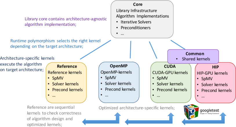
Figure 1. Ginkgo library architecture separating the core containing the algorithms from architecture-specific backends.

The object-oriented Ginkgo library is constructed around two principal design concepts. The first principle, aiming at future technology readiness, is to consequently separate the numerical algorithms from the hardware-specific kernel implementation to ensure correctness (via comparison with sequential reference kernels), performance portability (by applying hardware-specific kernel optimizations), and extensibility (via kernel backends for other hardware architectures), see Figure 1. The second design principle, aiming at user-friendliness, is the convention to express functionality in terms of linear operators: every solver, preconditioner, factorization, matrix-vector product, and matrix reordering is expressed as a linear operator (or composition thereof).

The rest of the paper is organized as follows. In Section 2, we leverage a simple use case to motivate the design choices underlying Ginkgo, and elaborate on the concept of linear operators, memory management, hardware-specific kernel optimization, and event logging. Section 3 provides additional details on Ginkgo’s current solvers, realizations for the sparse matrix-vector product (SpMV) kernel, and preconditioner capabilities. Section 4 elaborates on how the design allows for easy extension, so that users can contribute new algorithmic technology or additional hardware backends. As many applications are in desperate need for high performance sparse linear algebra technology, Section 5 showcases the usage of Ginkgo as a backend library in scientific applications, and also reviews Ginkgo’s integration into the extreme-scale Software Development Kit (xSDK). In Section 6 we describe how Ginkgo’s design and development cycle promotes sustainable software development; and in Section 7, we offer representative performance results indicating Ginkgo’s competitiveness for sparse linear algebra on high-end GPU architectures. We conclude in Section 8 with a summary of the paper and the potential of the library design becoming a role model for future developments.

2. An Overview of Ginkgo’s design

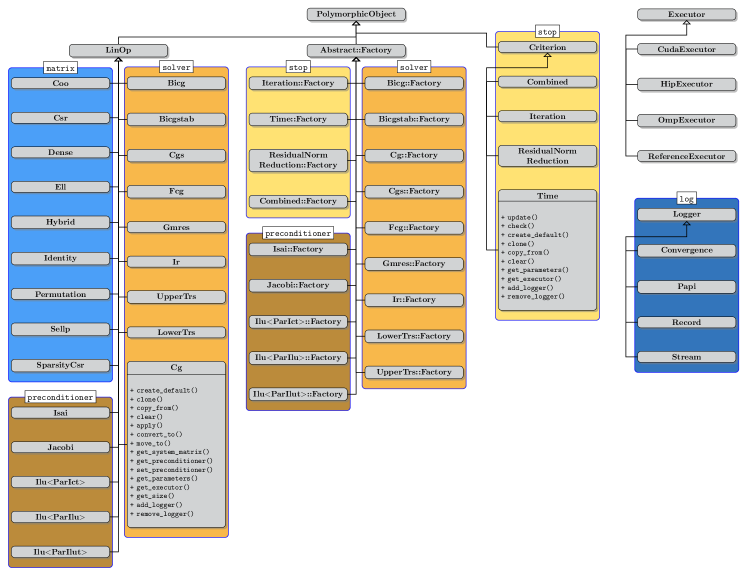
Figure 2. Ginkgo’s class hierarchy showcasing the main namespaces (colored boxes) and classes (gray boxes) for Ginkgo.

Figure 2 displays Ginkgo’s rich class hierarchy together with its main namespaces and classes. To better understand the role of each object, this section introduces Ginkgo’s interface using a minimal, concrete example as a starting point, and gradually presenting more advanced abstractions that demonstrate Ginkgo’s high composability and extensibility. These abstractions include:

• the LinOp and LinOpFactory classes which are used to implement and compose linear algebra operations,

• the Executor classes that allow transparent algorithm execution on multiple devices; and

• other utilities such as the Criterion classes, which control the iteration process, as well as the memory passing decorators that allow fine-grained control of how memory objects are passed between different components of the library and the application.

2.1. Ginkgo usage example

Figure 3 illustrates the specific flowchart Ginkgo uses to solve a linear system, highlighting the interactions between Ginkgo’s classes. In the program code for this example given in LABEL:lst:gko_code, the system matrix A, the right-hand side b, and the initial solution guess x, are initially read from the standard input using Ginkgo’s ‘read’ utility (lines 9–11). Next, the program creates a factory for a CG Krylov solver preconditioned with a block-Jacobi scheme (lines 13–15). The solver is configured to stop either after 20 iterations or having improved the original residual by 15 orders of magnitude (lines 16–19). (Stopping criteria are further discussed in Section 2.5.) The system matrix is bound to the iterative solver, which is used to solve the system with the right-hand side and initial guess. The initial guess is overwritten with the computed solution (line 23). Solvers (and more generally LinOp and LinOpFactory) are discussed in detail in Section 2.2. Finally, the solution is printed to the standard output (line 25).

⬇

1#include <iostream>

2#include <ginkgo/ginkgo.hpp>

3

4int main()

5{

6 // Instantiate a CUDA executor

7 auto cuda = gko::CudaExecutor::create(0, gko::OmpExecutor::create());

8 // Read data

9 auto A = gko::read<gko::matrix::Csr<>>(std::cin, cuda);

10 auto b = gko::read<gko::matrix::Dense<>>(std::cin, cuda);

11 auto x = gko::read<gko::matrix::Dense<>>(std::cin, cuda);

12 // Create the solver factory

13 auto solver_factory =

14 gko::solver::Cg<>::build()

15 .with_preconditioner(gko::preconditioner::Jacobi<>::build().on(cuda))

16 .with_criteria(

17 gko::stop::Iteration::build().with_max_iters(20u).on(cuda),

18 gko::stop::ResidualNormReduction<>::build()

19 .with_reduction_factor(1e-15)

20 .on(cuda))

21 .on(cuda);

22 // Create the solver from the factory and solve the system

23 solver_factory->generate(gko::give(A))->apply(gko::lend(b), gko::lend(x));

24 // Write result

25 write(std::cout, gko::lend(x));

26}

Listing 1: A minimal example that uses Ginkgo to solve a linear system. The system matrix, right-hand side, and the initial solution guess are read from the standard input. The system is solved on an NVIDIA-enabled GPU using the CG method enhanced with a block-Jacobi preconditioner. Two stopping criteria are combined to limit the maximum number of iterations and set the desired relative error. The solution is written to the standard output.

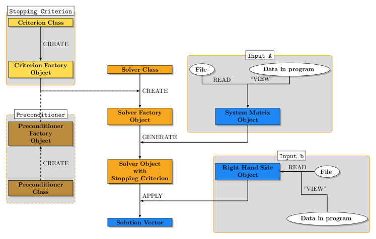
Figure 3. Flowchart providing an alternative view of the code example shown in LABEL:lst:gko_code. All object interactions are represented by arrows. The colors correspond to the type of the objects following the color convention in Figure 2.

Ginkgo supports execution on GPU and CPU architectures using different backends (currently, CUDA, HIP, and OpenMP). To accommodate this, when creating an object, the user passes an instance of an Executor in order to specify where the data for that object should be stored and the operations on that data should be performed. The particular example in LABEL:lst:gko_code creates a CUDA Executor (line 7) that employs the first GPU device (the one returned by cudaGetDevice(0)). Since CUDA GPU accelerators are controlled by the CPU, an OpenMP Executor is needed to orchestrate the execution on the GPU. (Section 2.3 describes the executors model in more detail.)

Ginkgo avoids expensive memory movement and copies. At the same time, sharing data between different modules in the code might cause unexpected results (e.g., one module changes a matrix used by a solver in a different module, which causes that solver to tackle the wrong system). Ginkgo resolves the dilemma by allowing both shared and exclusive (unique) ownership of the objects. This comes at the price of some verbosity in argument passing: in most cases, plain arguments cannot be passed directly, but have to be wrapped in special “decorator” functions that specify in which “mode” they are passed (shared, copied, etc.).

The minimal example in LABEL:lst:gko_code already utilizes two of the decorator functions, gko::give and gko::lend, both in line 23. The first one, gko::give(A), causes the caller to yield the ownership of matrix A to the solver, leaving the caller’s version of A in a valid, but undefined state (e.g., accessing any of its methods is not defined, but the object can still be de-allocated or assigned to). The second decorator, appearing twice, in gko::lend(x) and gko::lend(b), “lends” objects x and b to the solver by temporarily passing ownership to it until the control flow returns from apply back to the caller. This is a special ownership mode that is only used when the callee does not need permanent ownership of the object. Different ownership modes, as well as their relation to std::move are discussed in Section 2.4.

2.2. LinOp and LinOpFactory

2.2.1. Motivation

Ginkgo exposes an application programming interface (API) that allows to easily combine different components for the iterative solution of linear systems: solvers, matrix formats, preconditioners, etc. The API enables running distinct iterative solvers and enhancing the solvers with different types of preconditioners. A preconditioner can be a matrix or even another solver. Furthermore, the system matrix does not need to be stored explicitly in memory, but can be available only as a function that is applied to a vector to compute a matrix-vector product (matrix-free). The objective of providing a clean and easy-to-use interface mandates that all these special cases are uniformly realized in the API.

The central observation that guides Ginkgo’s design is that the operations and interactions between the solver, the system matrix, and the preconditioner can be represented as the application of linear operators:

1. The major operation that an iterative solver performs on the system matrix A is the multiplication with a vector (realized as a Matrix-Vector product, or MV). This operation can be viewed as the application of the induced linear operator $L_{A}:z\mapsto Az$. In some cases, multiplication with the transpose is also needed, which is yet another application of a linear operator $L_{A^{T}}:z\mapsto A^{T}z$.

2. The solver itself solves a system $Ax=b$, which is the application of the linear operator $S_{A}:b\mapsto A^{-1}b(=x)$. Here, the term “solver” is not used to denote a function $f$ that takes $A$ and $b$ as inputs and produces $x$, but instead a function with the system matrix $A$ already fixed (that is, $S_{A}=f(A\,,\cdot)$).

3. The application of the preconditioner $M$, as in $v=M^{-1}u$, can be viewed as the application of the linear operator $P_{M}:u\mapsto M^{-1}u(=v)$.

There are several remarks that have to be made regarding the observations above. First, in the context of numerical computations, with finite precision arithmetic, the term “linear operator” should be understood loosely. In fact, none of the previous categories strictly satisfy the linearity definition of the linear operator: $L(\alpha x+\beta y)=\alpha L(x)+\beta L(y)$, where $\alpha,\beta$ are scalars and $x,y$ denote vectors. Instead, they are just approximations of the linear operators that satisfy the formula $L(\alpha x+\beta y)=\alpha L(x)+\beta L(y)+E$, where the error term $E=E(L,\alpha,\beta,x,y)$ is the result of one or more of the following effects:

1. rounding errors introduced by storing non-representable values in floating-point format;

2. rounding errors introduced by finite-precision floating-point arithmetic;

3. instability and inaccuracy of the method used to apply the linear operator to a vector; and

4. inexact operator application, e.g. only few iterations of an iterative linear solver.

The data layout and the implementation of any linear operator is internal to that operator, and the interface does not expose implementation details. For example, a direct solver could store its matrix data in factored form, as two triangular factors (e.g., $A=LU$) and implement its application as two triangular solves (with $L$ and $U$). In contrast, an iterative solver could just store the original system matrix, and the entire implementation of the method could be a part of the linear operator application. Nonetheless, both operators can still expose the same public interface.

2.2.2. LinOp

In coherence with the observations in Section 2.2.1, the central abstraction in Ginkgo’s design is the abstract class (interface) LinOp, which represents the mathematical concept of a linear operator. All concrete linear operators (solvers, matrix formats, preconditioners) are instances of LinOp. Furthermore, this generic operator $L$ exposes a pure virtual method apply(b, x) that is overridden by a concrete linear operator with an implementation that computes the result $x=L(b)$ with conformal dimensions for $L$, $x$ and $b$, where vectors are interpreted as dense matrices of dimension $n\times 1$. This design enables that a single interface can be leveraged to compute an MV with different matrix formats, the application of distinct types of preconditioners, the solution of linear systems using various solvers, or even the application of a user-defined linear operator.

Using the LinOp abstraction, an iterative solver can be implemented via references to other LinOps that represent the system matrix and the preconditioner. The solver does not have to be aware of the type of the matrix or the preconditioner — it is sufficient to know that they are both conformal with the LinOp interface. This means that the same implementation of the solver can be configured to integrate various preconditioners and matrices. Furthermore, the linear operator abstraction can also be used to compose “cascaded” solvers where the preconditioner can be replaced by another, less accurate solver, or even to create matrix-free methods by supplying a specialized operator as the system matrix, without explicitly storing the matrix.

2.2.3. LinOpFactory

LinOp exposes a uniform interface to different types of linear algebra operations. A missing piece in the puzzle is how these LinOps are created in the first place. For example, in order to solve a system with a matrix $A$ represented by the linear operator $L_{A}$, an operation has to be provided which, given the operator $L_{A}$, creates a solver operator $S_{A}$. Similarly, to create a preconditioner $P_{A}$ for a matrix $A$, an operator that maps $L_{A}$ to $P_{A}$ is needed. These are both examples of higher-order (non-linear) functions that map linear operators to other linear operators (in this case $\Sigma:L_{A}\mapsto S_{A}$ and $\Phi:L_{A}\mapsto P_{A}$). Ginkgo provides an abstract class LinOpFactory that represents mappings such as $\Sigma$ and $\Phi$. Concretely, the class LinOpFactory provides an abstract method generate(LinOp) which, given a linear operator from the domain of the mapping, returns the corresponding LinOp from its input.

The linear operators constructed by using operator factories are usually solvers and preconditioners. For example, in order to construct a BiCGSTAB solver operator that solves a problem with the system matrix $A$, represented by the operator $L_{A}$, one would first create a BiCGSTAB factory (which implements the LinOpFactory interface and represents the operator $S$); and then call generate on $S$, passing the operator $L_{A}$ as input, to obtain a BiCGSTAB operator $S_{A}$, with the system matrix, $A$.

Some factories are designed to be combined with other factories. For instance, to create an iterative refinement solver, which uses CG preconditioned with Jacobi as the inner solver, one would create an iterative refinement factory $S$, and as the inner solver factory, pass a CG factory constructed with a Jacobi factory as the preconditioner factory. Then, when calling the generate method on $S$ with the system matrix represented by a linear operator $L_{A}$, this linear operator is propagated to the CG and Jacobi factories, to create CG and Jacobi operators with the system matrix $A$.

Instead of using LinOpFactory, an alternative (and more obvious) approach would have been to just use the constructor of LinOp to provide all the “component” linear operators. However, this alternative presents the drawback that the “type” of the operator cannot be decoupled from its data. To illustrate this, consider the scenario of a solver $S$ which tackles a linear system using the LU factorization; and then invokes two triangular solvers on the resulting $L$ and $U$ factors. There are multiple algorithms for the solution of the triangular systems, which in Ginkgo are represented by different linear operators. Thus, the operators to use should somehow be passed as input parameters to the solver $S$. The problem is that they cannot be constructed outside of $S$, since their factors are not known at that point. LinOpFactory provides an elegant solution to this problem, since instead of a LinOp, the solver $S$ can be provided with linear operator factories, which are then used to construct the triangular solver operators once the factors $L$ and $U$ are known.

2.2.4. Re-visiting the example

After the previous elaboration on LinOp and LinOpFactory, it is timely to re-visit the example in LABEL:lst:gko_code. The objects A, b and x in lines 9–11 are LinOp objects that store their data as “matrices” in CSR (compressed sparse row (Saad, 2003)) and dense matrix formats, respectively. Calling the method apply on these objects has the effect of calculating the matrix-vector product using that data. The solver_factory object (defined in lines 13–21), is actually a compound LinOpFactory used to create a solver with the CG method. In this particular case, the CG solver is preconditioned with a block-Jacobi method (specified by providing a block-Jacobi factory as the preconditioner factory to the CG factory).

All the work actually occurs in line 23. First, the CG factory solver_factory is used to generate a linear operator object representing the CG solver by calling the generate method. Since solver_factory has a block-Jacobi factory set as the preconditioner factory, the solver_factory’s generate method invokes generate on the block-Jacobi factory; and the system matrix A is passed as input argument, which has the effect of generating a block-Jacobi preconditioner operator for that matrix. Then, the resulting linear operator is immediately used to solve the system by applying it on b. This will have the effect of iterating the CG solver preconditioned with the generated block-Jacobi preconditioner operator on the system matrix A, thus solving the system.

2.2.5. Linear operator algebra

Traditional linear algebra libraries, such as BLAS (Lawson et al., 1979) and LAPACK (Anderson et al., 1999), use vectors and matrices as basic objects, and provide operations such as matrix products and the solution of linear systems on these objects as functions. In contrast, Ginkgo achieves composability and extensibility (cf. Section 4) by treating linear operations as basic objects, and providing methods to manipulate these operations in order to express the desired complex operation. This is the principle guiding the design of Ginkgo, which motivates the title of this paper: while other libraries can be characterized as “linear algebra libraries”, Ginkgo’s algebra is performed on linear operators, making it a “linear operator algebra library”.

While the current focus of Ginkgo is on the iterative solution of sparse linear systems, other types of operations on linear operators also fit into Ginkgo’s concept of LinOp and LinOpFactory. For example, a matrix factorization $A=UV$ can be viewed as a linear operator factory $\Psi:L_{A}\mapsto F_{U,V}$, where the linear operator $F_{U,V}:b\mapsto UVb$ stores the two factors $U$ and $V$, and provides public methods to access the factors.

2.3. Executors for transparent kernel execution on different devices

An appealing feature of Ginkgo is the ability to run code on a variety of device architectures transparently. In order to accommodate this functionality, Ginkgo introduces the Executor class at its core. In consequence, the first task a user has to do when using Ginkgo is to create an Executor.

The Executor specifies the memory location and the execution space of the linear algebra objects and represents computational capabilities of distinct devices. Currently, four executor types are provided:

• CudaExecutor for CUDA-enabled GPUs;

• HipExecutor for HIP-enabled GPUs;

• OmpExecutor for OpenMP execution on multicore CPUs; and

• ReferenceExecutor for sequential execution on CPUs (used for correctness checking).

Each of these executors implements methods for allocating/deallocating memory on the device targeted by that executor, copying data between executors, running operations, and synchronizing all operations launched on the executor.

LABEL:lst:gko_code illustrated the use of Executor. Combined with the gko::clone(Executor, Object) utility function, the Executor class makes it straight-forward to move all data and operations to a host OpenMP executor, as in LABEL:lst:gko_matrix_copy_example. That code creates an gko::OmpExecutor object for execution on the CPU (line 1). Next, a CUDA executor representing a GPU device with ID 0 is created (line 2); and the system matrix data is read from a file and allocated on the gko::CudaExecutor’s device memory (line 4). Finally, the function gko::clone creates a copy of A on the gko::OmpExecutor, that is, in the platform’s main memory (line 6).

⬇

1 auto omp = gko::OmpExecutor::create();

2 auto cuda = gko::CudaExecutor::create(0, omp);

3 // As in previous example, A is allocated on a CUDA device

4 auto A = gko::read<gko::matrix::Csr<>>("data/A.mtx", cuda);

5 // copy A to an OpenMP-capable device

6 auto A_copy = gko::clone(omp, A);

7 // All subsequent operations triggered from A_copy will use executor omp

Listing 2: Copy of a matrix in CSR format from a CUDA device to a CPU through the OmpExecutor.

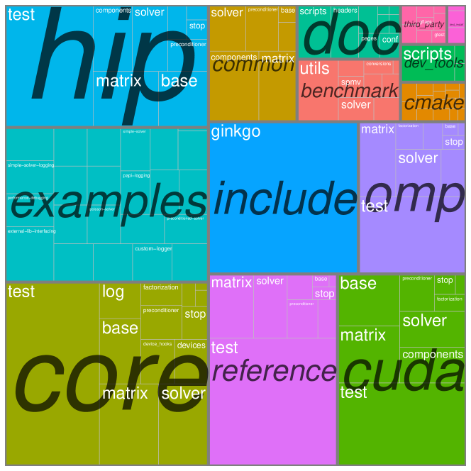
Figure 4. Code distribution among different modules in Ginkgo develop version 1.1.1. The entire code base in this release is 8.0 MB (represented by the entire figure). The top level rectangles represent different top-level directories; these are: the core (1.4 MB) module, examples (1.2 MB), the HIP module (928 KB), the CUDA module (920 KB), the reference module (924 KB), the include directory with the core module’s public headers (852 KB), the omp module (612 KB), the common directory which contains shared HIP and CUDA kernels (388 KB) and the benchmark (244 KB) and doc directories (212 KB each). The first rectangles in the core, CUDA, HIP, omp and reference modules represent unit tests for these modules, which amount to 644, 396, 400, 308 and 612 KB, respectively.

In order to allow a transparent execution of operations on multiple executors, the kernels in Ginkgo have separate implementations for each executor type, organized into several modules, see Figure 1 and Figure 4 for the code distribution, respectively. The core module contains all class definitions and non-performance critical utility functions that do not depend on an executor. In addition, there is a module for each executor, which contains the kernels and utilities specific for that executor. Each module is compiled as a separate shared library, which allows to mix-and-match modules from different sources. This paves the road for hardware vendors to provide their own proprietary modules: they only have to optimize their module, make it available in binary form, and users can then link it with Ginkgo. We note that the similarities between HIP and CUDA allow the usage of common template kernels that are identical in kernel design but are compiled with architecture-specific parameters to either the HipExecutor or the CudaExecutor. This strategy reduces code replication and favors productivity and maintainability.

Ginkgo contains dummy kernel implementations of all modules that throw an exception whenever they are called. This allows a user to deactivate certain modules if no hardware support is available or to reduce compilation time. In general, during the configuration step, Ginkgo’s automatic architecture detection activates all modules for which hardware support has been detected.

The Executor design allows switching the target device where the solver in LABEL:lst:gko_code is executed through a one-line change that replaces the executor used for it. In addition, if one of the arguments for the apply method is not on the same executor as the operator being applied, the library will temporarily move that argument to the correct executor before performing the operation, and return it back once the operation is complete. Even though this is done automatically, the user may attain higher performance by explicitly moving the arguments in order to avoid unnecessary copies (in the case, for example, of repeated kernel invocation).

2.4. Memory management

Libraries have to specify several key memory management aspects: memory allocation, data movement and copy, and memory deallocation. In contrast to traditional libraries such as BLAS and LAPACK, which leave memory management to the user, Ginkgo allocates/deallocates its memory automatically, using the C++ “Resource Acquisition Is Initialization” (RAII) concept combined with the native allocation/deallocation functions of the executor (cf. Section 2.3). Alternatively, to eliminate unnecessary allocations and data copies, Ginkgo’s matrix formats can be configured to use raw data already allocated and managed by the application by using Array views.

A more difficult problem is to realize data movement and copies between different entities of the application (e.g., functions and other objects). The memory management has to not only protect against memory leaks or invalid memory deallocations, but also avoid unnecessary data copies. The problem is usually solved by specifying a well-defined owner for each object, responsible for deallocating the object once it is no longer needed.

For simple C++ types, this behavior is enabled via the use of parameter qualifiers: Parameters are passed by-value and thus copied unless explicitly declared as references (which is when they are passed by-reference without copying). The C++11 standard added move semantics as a third alternative where an input parameter that is either explicitly (using std::move) or implicitly (by not having a name) designated a temporary value may move its internal data into the function without copying, leaving it in a valid but unspecified state. However, trying to pass polymorphic objects by-value would lead to object slicing (obj, 2020). In Ginkgo, we avoid these issues with polymorphic types like Executor and LinOp by always passing and returning them as pointers. To this goal, we use the smart pointer types std::unique_ptr and std::shared_ptr, which were added in the C++11 standard. They provide safe resource management using RAII while still providing (almost) the same semantics as raw pointers. Ginkgo uses pointers for parameters and return types in three different contexts, where we say that a function parameter is used in a non-owning context if the object will only be used during the function call, and in an owning context if the object needs to be accessible even after the function call completed. Figure 5 shows the different ways to pass a polymorphic object as a parameter in Ginkgo.

Functions that only need to modify a polymorphic object in a non-owning context take this object as a raw pointer parameter T*. To simplify the interaction with smart pointers, Ginkgo provides the overloaded gko::lend function which returns the underlying raw pointer for both smart and raw pointers. This decorator function allows for a concise and uniform way to pass polymorphic objects to functions without ownership transfer. “Lending” an object can be compared with normal by-reference semantics for value types. When by-value semantics are necessary, we can explicitly pass a copy using gko::lend(gko::clone($\cdot$)).

Functions that need to receive a polymorphic object in an owning context take this object as a std::shared_ptr<T>. We can pass an object to such a parameter in three ways: gko::clone creates a copy of the current object to be passed to the function (by-value), gko::give specifies that the object will not be used afterwards and can thus be moved into the function (move semantics) and gko::share specifies that the ownership should be shared with the function (by-reference). Note that the gko::share annotation can usually be left out, since all owning smart pointers in C++ already provide conversions to std::shared_ptr.

Functions that create new instances of a polymorphic object return a std::unique_ptr<T>, while access to already existing objects is provided with std::shared_ptr<const T> to allow the objects to be used in both owning and non-owning contexts.

The overloaded decorator functions gko::clone, gko::lend, gko::give and gko::share provide a uniform interface for all types of smart and raw pointers, while still ensuring type safety. For example, calling gko::give with a non-owning pointer will fail to compile and output an appropriate error message.

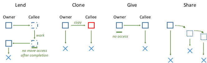
Figure 5. Different ways of passing polymorphic objects as parameters in Ginkgo:
gko::clone, gko::lend, gko::give, gko::share together with the lifetime of the passed object.

2.5. Control of the iteration process

Virtually all iterative methods include the concept of a “stopping criterion” that evaluates whether the current approximation to the solution of the linear systems is accurate enough. To facilitate controlling the iteration process, Ginkgo provides a collection of stopping criteria. All of them are implementations of the base Criterion class, which specifies what type of information can be passed to the stopping criterion. A concrete criterion provides an implementation of the check() method that verifies if its condition has been met and, therefore, the iteration process has to be stopped.

The stopping criteria are initially generated from criterion factories (created by the user) by passing the system matrix, right-hand side, and an initial guess. In addition, during the iteration process, information can be updated when calling the check() function with the new iteration count, residual, solution or residual norm.

Currently, three basic stopping criteria are provided in Ginkgo:

• The Time criterion, which automatically stops the iteration process after a certain amount of time;

• the Iteration criterion, which stops the iteration process once a certain iteration count has been reached; and

• the ResidualNormReduction criterion, which stops the iteration process once the initial relative residual norm has been reduced by the certain specified amount.

Additionally, Ginkgo provides a Combined criterion, which can be used to combine multiple criteria together through a logical–OR operation (|), so that the first subcriterion that is fulfilled stops the iteration process. This is illustrated in lines 16–19 of LABEL:lst:gko_code. This design implies some stopping criteria may detain the iteration process before “convergence” is reached, in particular the Time and Iteration criteria. Ginkgo provides a stopping_status class, which can be inspected to find out which criterion stopped the iteration process.

The Criterion class hierarchy is designed to avoid negative impact on the performance, and may even improve it. For example, in case an iterative method is applied with multiple right-hand side vectors, the stopping_status is evaluated for each right-hand side individually, skipping vector updates in subsequent iterations for those right-hand side vectors where convergence has been achieved.

Also, all operations required to control the iteration process can be handled inside the Criterion classes. The consequence is that, for most solvers, the residual norm and related operations are computed only when using the ResidualNormReduction criterion. Therefore, the user can combine a solver with a simple stopping criterion to make it more lightweight or choose a more precise but more expensive stopping criterion. In summary, Ginkgo’s design of stopping criteria tries to honor the C++ philosophy of “only paying for what you use”.

2.6. Event logging

Another utility that is provided to users in Ginkgo is the logging of events with the purpose to record information about Ginkgo’s execution. This covers many aspects of the library, such as memory allocation, executor events, LinOp events, stopping criterion events, etc. For ease of use, the event logging tools provide different forms of output formats, and allow the usage of multiple loggers at once. As with the rest of Ginkgo, this tool is designed to be controllable, extensible, and as lightweight as possible. To offer support for all those capacities, the Logger infrastructure follows the visitor and observer design patterns (Gamma et al., 1994). This design implies a minimal impact of logging on the logged classes and allows to accommodate any logger.

The following four loggers are currently provided in Ginkgo:

• the Stream logger, which logs the events to a stream (e.g., file, screen, etc.);

• the Record logger, which stores the events in a structure which has a history of all received events that the user can retrieve at any moment;

• the Convergence logger is a simple mechanism that stores the relative residual norm and number of iterations of the solver on convergence; and

• the PAPI SDE logger uses the PAPI Software Defined Events backend (Jagode et al., 2019) in order to enable access to Ginkgo’s internal information through the PAPI interface and tools.

Almost every class in Ginkgo possesses multiple corresponding logging events. The logged classes are: Executor, Operation, PolymorphicObject, LinOp, LinOpFactory and Criterion. The user has the freedom to choose whether he/she wants to log all events or select only some of them. When an event is not selected for logging by the user, as a result of the implementation of the logging facilities, the event is not propagated and generates a “no-op”.

3. Using Ginkgo as a library

3.1. Solver

Currently, Ginkgo provides a list of Krylov solvers (BICG, BiCGSTAB, CG, CGS, FCG, GMRES) for the iterative solution of sparse linear systems, fixed-point methods, and direct solvers for sparse triangular systems such as those that appear in incomplete factorization preconditioning. In order to generate a solver, a solver factory (of type LinOpFactory) must first be created, where solver control parameters, such as the stopping criterion, are set. The concrete solver is then generated by binding the system matrix to the solver factory. This allows to generate multiple solvers for distinct problems with the same solver settings, e.g. in time-stepping methods. Except for Iterative Refinement (IR), where the internal solver can be chosen, all iterative solvers have the option to attach a preconditioner of the class LinOp. Furthermore, all solvers implement the abstract LinOp interface, which not only simplifies the solver usage, but also allows to use the same notation for calling solvers, preconditioners, SpMV, etc. This allows the user to compose iterative solvers by choosing another iterative solver as a preconditioner.

3.2. Preconditioner

Ginkgo allows any solver to be used as a preconditioner, i.e., to cascade Krylov solvers. Additionally, Ginkgo features diagonal scaling preconditioners (block-Jacobi) as well as incomplete factorization (ILU-type) preconditioners. As any of the other solvers, preconditioners are generated through a LinOpFactory and implement the abstract class LinOp.

The block-Jacobi preconditioners can switch between a “standard” mode and an “adaptive precision” mode (Anzt et al., 2019c). In the latter case, the memory precision is decoupled from the arithmetic precision, and the storage format for each inverted diagonal block is optimized to preserve the numerical properties while reducing the memory access cost (Flegar et al., tted).

The ILU-based preconditioners can be generated by interfacing vendor libraries, via the ParILU algorithm (Chow et al., 2015), or via a variant known as the ParILUT algorithm (Anzt et al., 2018a) that dynamically adapts the sparsity pattern of the incomplete factorization to the problem characteristics (Anzt et al., 2019d).

For the application of an ILU-type preconditioner, Ginkgo leverages two distinct solvers: one for the lower triangular matrix $L$ and one for the upper triangular matrix $U$. The default choices are the direct lower and upper triangular solvers but the user can change this to use iterative triangular solves.

In LABEL:lst:ilu-preconditioner-custom we illustrate how an ILU preconditioner can be customized in almost all aspects. In this case, we select a CGS solver for solving the upper triangular system by first creating the factory in lines 18–23 and then attaching it to the preconditioner factory in lines 26–28. Instead of relying on the internal generation of the incomplete factors, we generate them ourselves in lines 13–15. Afterwards, we generate the ILU preconditioner in line 29. In the end, we employ the now already generated preconditioner in line 40 with a BiCGSTAB solver.

⬇

1#include <iostream>

2#include <ginkgo/ginkgo.hpp>

3

4int main()

5{

6 // Instantiate a CUDA executor

7 auto cuda = gko::CudaExecutor::create(0, gko::OmpExecutor::create());

8 // Read data

9 auto A = gko::read<gko::matrix::Csr<>>(std::cin, cuda);

10 auto b = gko::read<gko::matrix::Dense<>>(std::cin, cuda);

11 auto x = gko::read<gko::matrix::Dense<>>(std::cin, cuda);

12 // Generate ILU(0) factorization

13 auto ilu_factorization =

14 gko::factorization::ParIlu<>::build().on(cuda)

15 ->generate(A);

16 // Create a custom upper solver factory

17 auto upper_solver_factory =

18 gko::solver::Cgs<>::build()

19 .with_criteria(

20 gko::stop::ResidualNormReduction<>::build()

21 .with_reduction_factor(1e-5)

22 .on(cuda))

23 .on(cuda);

24 // Create an ILU preconditioner factory with a CGS upper solver

25 auto ilu_factory =

26 gko::preconditioner::Ilu<gko::solver::LowerTrs<>, gko::solver::Cgs<>>::build()

27 .with_u_solver_factory(gko::share(upper_solver_factory))

28 .on(cuda);

29 auto ilu_prec = ilu_factory->generate(gko::share(ilu_factorization));

30 // Create the solver factory with ILU preconditioning

31 auto solver_factory =

32 gko::solver::Bicgstab<>::build()

33 .with_criteria(

34 gko::stop::ResidualNormReduction<>::build()

35 .with_reduction_factor(1e-15)

36 .on(cuda),

37 .with_generated_preconditioner(gko::share(ilu_prec))

38 .on(cuda);

39 // Create the solver from the factory and solve the system

40 solver_factory->generate(gko::give(A))->apply(gko::lend(b), gko::lend(x));

41 // Write result

42 write(std::cout, gko::lend(x));

43}

Listing 3: An example of creating a CG solver with ILU preconditioning with an iterative solver for the upper triangular factor.

4. Using Ginkgo as a framework

As described in Section 2, Ginkgo provides a set of generic linear operators, including various general matrix formats, popular solvers, and simple preconditioners. However, sparse linear algebra often includes problem-specific knowledge. This means that, in general, a highly-optimized implementation of a generic algorithm will still be outperformed by a carefully crafted custom algorithm employing application-specific knowledge. To tackle this, Ginkgo promotes extensibility so that users can develop their own implementation for specific functionality without needing to modify Ginkgo’s code (or recompile it).

Domain-specific extensions can be elaborated as part of the application that uses them, or even bundled together to create an ecosystem around Ginkgo. Currently, this is possible for all linear operators, stopping criteria, loggers, and corresponding factories. Adding custom data types also requires only minor changes in a single header file and a recompilation. The only extension that requires more significant efforts is the addition of new architectures and executors. This involves modifying a key portion of Ginkgo as it requires the addition of specialized implementations of all kernels for the new architecture and executor.

In contrast to the previous section, where Ginkgo is used as a library and the application is built around it, this section describes how Ginkgo can be used as a framework in which the application inserts its own custom components to work in harmony with Ginkgo’s built-in technology.

4.1. Utilities supporting extensibility

Ginkgo’s facilities for memory management (e.g., automatic allocation and deallocation, or transparent copies between different executors) are designed to simplify its use as a library. As a result, the implementation burden is then shifted to the developers of these facilities, which are either the developers of Ginkgo or, in case the application using Ginkgo needs custom extensions, the developers of that application. To alleviate the burden and help developers focus on their algorithms, Ginkgo provides basic building blocks that handle memory management and the implementation of interfaces supported by the component being developed.

4.1.1. Array

Most components in Ginkgo have some sort of associated data, which should be stored together with its executor. When copying a component, its data should also be copied, possibly to a different executor. When the object is destroyed, the data should be deallocated with it. Doing this manually for every class introduces a large amount of boilerplate code, which increases the effort of developing new components, and can lead to subtle memory leaks. In addition, different devices have different APIs for memory management, so a separate version would have to be written for each executor.

To handle these issues in a single point in code, while removing some of the burden from the developer, Ginkgo provides the Array class. This is a container which encapsulates fixed-sized arrays stored on a specific Executor. It supports copying between executors and moving to another executor. In addition, it leverages the RAII idiom to automatically deallocate itself from the memory when it is no longer needed.

⬇

1auto omp = gko::OmpExecutor::create();

2auto cuda = gko::CudaExecutor::create(0, omp);

3using arr = gko::Array<int>;

4

5arr x(cuda, {1, 2, 3, 4}); // an array of integers on the GPU

6arr cpu_x(omp, x); // a copy of x on the CPU

7arr z(omp, 10); // an uninitialized array of 10 integers on the CPU

8

9z = x; // copy x from the GPU to z (on the CPU)

10z.set_executor(cuda); // move z to the GPU

11

12auto d[] = {1, 2, 3, 4};

13auto d_arr = arr::view(omp, 4, d); // use existing data

14

15auto size = x.get_num_elems(); // get the size of x

16auto x_data = x.get_data(); // get raw pointer to x’s data

17// Note that x_data[0] would cause a segmentation fault if called from the CPU.

18// Memory used for x, cpu_x and z is automatically deallocated.

19// d_arr does not try to deallocate the memory.

Listing 4: Usage examples of the Array class.

LABEL:lst:gko_array_example shows some common usage examples of arrays. Lines 5–7 display several ways of initializing the Array: using an initializer list, copying from an existing array (from a different executor), or allocating a specified amount of uninitialized memory. The last constructor will only allocate the memory, without calling the constructors on individual elements, which remains the responsibility of the caller. While this is not the usual behavior in C++, properly parallelizing the construction of the elements in multi- and manycore systems is a non-trivial task. Nevertheless, the elements of the arrays used in Ginkgo are mostly trivial types, so there is usually no need to call the constructor in the first place.

Lines 9–10 shown in LABEL:lst:gko_array_example illustrate how the assignment operator can be used to copy arrays and how the executor of the array can be changed via the set_executor method. The combination of the assignment operator and the RAII idiom usually means that classes using arrays as building blocks do not require user-defined destructors or assignment operators, since the ones synthesized by the compiler behave as expected (in particular, this is true for all of Ginkgo’s linear operators, stopping criteria, and loggers).

Lines 12–13 show that Array can also be used to store data in a non-owning fashion in a view, i.e., the data will not be de-allocated when the Array is destroyed. This feature is particularly useful when using Ginkgo to operate on data owned by the application or another library.

Finally, raw data stored in the Array can be retrieved as shown in Lines 15–17. The get_data method will return a raw pointer on the device where the array is allocated, so trying to dereference the pointer from another device will result in a runtime error.

4.1.2. Introduction to mixins

Most components in Ginkgo expose a rich collection of utility functions, usually related to conversion, object creation, and memory movement. These utilities are usually trivial to implement, and do not differ much between components. However, they still require that the developer implements them, which steers the focus away from the actual algorithm development. Ginkgo addresses this issue by using mixins (mix, 2020). Since those are neither well-known by the community nor well-supported in languages commonly used in high performance computing (e.g., C, C++, Fortran), this subsection provides a simple example where mixins are leveraged to reduce boilerplate code. The remaining parts of Section 4 introduce mixins provided by Ginkgo when extending certain aspects of its ecosystem.

As a toy example, assume there is an interface Clonable, which consists of a single method clone exposed to create a clone of an object. This method is useful if the object that should be cloned is only available through its base class (i.e., the static type of the object differs from its dynamic type). A common example where this is used is the prototype design pattern (Johnson et al., 1995). Obviously, the implementation of the clone method should just create a new object using the copy constructor. LABEL:lst:clonable-no-mixin is an example implementation of such a hierarchy consisting of three classes A, B and C. Classes A and B directly implement Clonable, while C indirectly implements it through B.

⬇

1struct Clonable {

2 virtual ~Clonable() = default;

3 virtual std::unique_ptr<Clonable> clone() const = 0;

4};

5

6struct A : Clonable {

7 std::unique_ptr<Clonable> clone() const override {

8 return std::unique_ptr<Clonable>(new A{*this});

9 }

10};

11

12struct B : Clonable {

13 std::unique_ptr<Clonable> clone() const override {

14 return std::unique_ptr<Clonable>(new B{*this});

15 }

16};

17

18struct C : B {

19 std::unique_ptr<Clonable> clone() const override {

20 return std::unique_ptr<Clonable>(new C{*this});

21 }

22};

Listing 5: An example hierarchy implementing clonable without the use of mixins.

The implementation of the clone method is almost identical in all classes, so it represents a good candidate for extraction into a mixin. Mixins are not supported directly in C++, so their implementation is handled via inheritance, usually coupled with the Curiously Recurring Template Pattern (CRTP) (Coplien, 1995). Nevertheless, using inheritance in this context should not be viewed as establishing a parent–child relationship between the mixin and the class inheriting from it, but instead as the class “including” the generic implementations provided by the mixin. LABEL:lst:clonable-with-mixin shows the implementation of the same hierarchy using the EnableCloning mixin designed to provide a generic implementation of the clone method. The mixin relies on the knowledge of the type of the implementer to call the appropriate constructor, which is provided as a template parameter. The base interface implemented by the mixin is also passed as a template parameter to allow indirect implementations, as is the case in class C. Once the mixin is set up, any class that wishes to implement Clonable can just include the mixin to automatically get a default implementation of the interface, making the class cleaner, and removing the burden of writing boilerplate code.

⬇

1struct Clonable {

2 virtual ~Clonable() = default;

3 virtual std::unique_ptr<Clonable> clone() const = 0;

4};

5

6template <typename Implementer, typename Base = Clonable>

7struct EnableCloning : Base {

8 std::unique_ptr<Clonable> clone() const override {

9 return std::unique_ptr<Clonable>(

10 new Implementer{*static_cast<const Implementer*>(this)});

11 }

12};

13

14struct A : EnableCloning<A> {};

15

16struct B : EnableCloning<B> {};

17

18struct C : EnableCloning<C, B> {};

Listing 6: An example hierarchy implementing clonable using the EnableCloning mixin.

Ginkgo uses mixins to provide default implementations, or parts of implementations of polymorphic objects, linear operators, various factories, as well as a few of other utility methods. To better distinguish mixins from regular classes, mixin names begin with the “Enable” prefix.

4.2. Creating new linear operators

The matrix structure is one of the most common types of domain-specific information in sparse linear algebra. For example, the discretization of the 1D Poisson’s differential equation with a 3-point stencil results in a tridiagonal matrix with a value $2$ for all diagonal entries and $-1$ in the neighboring diagonals. This special structure enables designing a matrix format which only needs to store the two values on and below/above the diagonal. Such compact matrix formats require far less memory than general ones, which directly translates into performance gains in the SpMV computation.

We adopt the example of the stencil matrix to demonstrate how to implement a custom matrix format. The code structure is shown in LABEL:lst:custom-matrix-format. The actual implementations of the OpenMP, CUDA, and reference kernels are not shown here for brevity as they do not use any important features of Ginkgo. A full implementation is available in Ginkgo’s custom-matrix-format example, which is included in Ginkgo’s source distribution.

Line 1 includes the EnableLinOp mixin, which implements the entire LinOp interface except the two apply_impl methods. These methods are called inside the default implementation of the apply method to perform the actual application of the linear operator. The default implementation of apply contains additional functionalities (executor normalization, argument size checking, logging hooks, etc.). Thus, by using the two-stage design with apply and apply_impl, the implementers of matrix formats do not have to worry about these details. Line 2 includes the EnableCreateMethod mixin, which provides a default implementation of the static create method. The default implementation will forward all the arguments to the StencilMatrix’ constructor, allocate and construct the matrix using the new operator, and return a unique pointer (std::unique_ptr) to the constructed object.

The constructor itself is defined in lines 4–8. Its parameters are the executor where the matrix data should be located and operations performed, the size of the stencil, and the three coefficients of the stencil. The executor and the size are handled by EnableLinOp, and the coefficients are stored in an Array (defined in line 55) located on the executor used by the matrix.

Linear operators provide two variants of the apply method. The “simple” version performs the operation $x=Ab$ and the “advanced” version for $x=\alpha Ab+\beta x$. Both of them are often used in linear algebra, and can be expressed in terms of each other: A “simple” application is just an “advanced” one with $\alpha=1$ and $\beta=0$. The “advanced” application can be expressed by combining $x$ and the result of “simple” application using the scal and axpy BLAS routines (called scale and add_scaled in Ginkgo). In general, specialized versions result in superior performance. Thus, Ginkgo provides both of them separately. However, for the sake of brevity, this example implements the “advanced” version in terms of the “simple” one (lines 14–42).

The remainder of the code (lines 15–57) contains the implementation structure of the “simple” application. The input parameters contain the input vector b and the vector x where the solution will be stored. Each input and solution vector is represented by one column of a linear operator. To accommodate future extensions (e.g., sparse matrix–sparse vector multiplication), both x and b are general linear operators. However, the only type supported by this example (and all of Ginkgo’s built-in operators) is matrix::Dense. Downcasting these vectors to matrix::Dense is realized in lines 15–16 using the gko::as utility, which throws an exception if one of them is not in fact a dense matrix.

The implementation of the apply operation depends on the hardware architecture. The Reference version uses a simple sequential CPU implementation; the OpenMP version relies on a parallel implementation based on OpenMP; and the CUDA and HIP versions launch a CUDA kernel and a HIP kernel, respectively. To support all four implementations, Ginkgo defines the Operation interface. An object that implements this interface is passed to the executor’s run method, which will select the appropriate implementation depending on the executor (lines 40–41). Thus, StencilMatrix has to define a class (called stencil_operation in this example, lines 18–39) which implements the Operation interface and encapsulates the four implementations. The implementations are placed into the four overloads of the run method: the reference version in lines 23–25; the OpenMP version in lines 26–28; the CUDA version in lines 29–31; and the HIP version in lines 32–34. References to the required data also have to be passed to stencil_operation so that the implementation can access it.

The new matrix format can be used instead of the CSR format in the example in LABEL:lst:gko_code by changing the definition of A in line 9 as shown in line 59 of LABEL:lst:custom-matrix-format, and placing the definition of $A$ after the definition of b. In addition, lines 14–15 defining the preconditioner have to be removed, since the block-Jacobi preconditioning requires additional functionalities of the matrix format.

Matrix formats are not the only linear operators that can be extended. A similar approach can be used to define new solvers and preconditioners.

⬇

1class StencilMatrix : public gko::EnableLinOp<StencilMatrix>,

2 public gko::EnableCreateMethod<StencilMatrix> {

3public:

4 StencilMatrix(std::shared_ptr<const gko::Executor> exec,

5 gko::size_type size = 0, double left = -1.0,

6 double center = 2.0, double right = -1.0)

7 : gko::EnableLinOp<StencilMatrix>(exec, gko::dim<2>{size}),

8 coefficients(exec, {left, center, right}) {}

9

10protected:

11 using vec = gko::matrix::Dense<>;

12 using coef_type = gko::Array<double>;

13

14 void apply_impl(const gko::LinOp *b, gko::LinOp *x) const override {

15 auto dense_b = gko::as<vec>(b);

16 auto dense_x = gko::as<vec>(x);

17

18 struct stencil_operation : gko::Operation {

19 stencil_operation(const coef_type &coefficients, const vec *b,

20 vec *x)

21 : coefficients{coefficients}, b{b}, x{x} {}

22

23 void run(std::shared_ptr<const gko::ReferenceExecutor>) const override {

24 // Reference kernel implementation

25 }

26 void run(std::shared_ptr<const gko::OmpExecutor>) const override {

27 // OpenMP kernel implementation

28 }

29 void run(std::shared_ptr<const gko::CudaExecutor>) const override {

30 // CUDA kernel implementation

31 }

32 void run(std::shared_ptr<const gko::HipExecutor>) const override {

33 // HIP kernel implementation

34 }

35

36 const coef_type &coefficients;

37 const vec *b;

38 vec *x;

39 };

40 this->get_executor()->run(

41 stencil_operation(coefficients, dense_b, dense_x));

42 }

43

44 void apply_impl(const gko::LinOp *alpha, const gko::LinOp *b,

45 const gko::LinOp *beta, gko::LinOp *x) const override {

46 auto dense_b = gko::as<vec>(b);

47 auto dense_x = gko::as<vec>(x);

48 auto tmp_x = dense_x->clone();

49 this->apply_impl(b, gko::lend(tmp_x));

50 dense_x->scale(beta);

51 dense_x->add_scaled(alpha, gko::lend(tmp_x));

52 }

53

54private:

55 coef_type coefficients;

56};

57

58// using the matrix format:

59auto A = StencilMatrix::create(exec, b->get_size()[0], -1.0, 2.0, -1.0);

Listing 7: Example implementation of a user-defined matrix format specialized for 3-point stencil matrices.

4.3. Creating new stopping criteria

Implementing new stopping criteria requires a deeper understanding of the concept than that explained in Section 2.5. To accommodate higher generality, a criterion is allowed to maintain state during the execution of a solver (e.g., a criterion based on a time limit may need to record the point in time when the solver was started). On the other hand, a linear operator may invoke a solver multiple times, every time its apply method is called. As a consequence, the same criterion cannot be reused for multiple runs, as the state from the previous invocation may interfere with a subsequent run. The solution is to prevent users from directly instantiating criteria. Instead, the user instantiates a criterion factory, which is then used by the solver to create a new criterion instance every time the solver is invoked. When creating the criterion, the solver will pass basic information about the system being solved, which includes the system matrix, the right-hand side, the initial guess, and optionally the initial residual. During its execution, the solver will call the criterion’s check method to decide whether to stop the process. This method receives a list of parameters that includes the current iteration number, and optionally one or more of the following: the current residual, the current residual norm, and the current solution. Based on this information, the criterion decides, separately for each right-hand side, whether the iteration process should be detained.

Currently, Ginkgo includes conventional stopping criteria for iterative solvers based on iteration count, execution time or residual thresholds, as well as mechanisms to combine multiple criteria. Nevertheless, users may achieve tighter control of the iteration process by defining their own stopping criteria. LABEL:lst:iteration-stopping-criterion offers a sample stopping criterion based on the number of iterations which, even though already available in Ginkgo as gko::stop::Iteration, is simple enough to show in full as part of this paper.

As mentioned in Section 2.5, all stopping criteria, including custom ones, should implement the Criterion interface. In addition to the check method, the interface provides various other utility methods which facilitate memory management. To reduce the volume of boiler-plate code needed for new stopping criteria, Ginkgo provides the EnablePolymorphicObject mixin. This mixin inherits an interface supporting memory management (in this case Criterion), and implements utility methods related to it (line 2). For the mixin to work properly, the class being enabled has to provide a constructor with an executor as its only parameter (lines 21–23).

Creating a criterion factory can be simplified by using the CREATE_FACTORY_PARAMETERS, FACTORY_PARAMETER and ENABLE_CRITERION_FACTORY macros. The first one creates a member type parameters_type, which contains all of the parameters of the criterion (lines 4–6). Each parameter is defined using the FACTORY_PARAMETER macro, which adds a data member of the requested name and default value, as well as a utility method “with_<parameter name>” that can be used when constructing the factory to set the parameter. In this case, the only parameter is the maximum number of iterations (line 5). Finally, the ENABLE_CRITERION_FACTORY macro creates a factory member type named Factory that uses the parameters to create the criterion. The macro also adds a data member parameters_ which holds those parameters (line 7). When used to instantiate a new criterion, the factory will pass itself, as well as an instance of parameters_type, to the constructor of the criterion. This constructor is defined in lines 25–29.

Finally, the implementation of the criterion logic is comprised inside the check method (lines 10–19). The current state of the solver is passed via the Updater object. This particular criterion uses the Updater::num_iterations property to check whether the limit on the number of iterations has been reached (line 13). If this is not the case, the criterion returns false, indicating to the solver that iterative process should continue (line 14). Otherwise, the stopping statuses of all columns are set (line 16), and the one_changed property is set to true to indicate that at least one of the statuses changed (lines 14–17). Finally, once the iteration process for all right-hand sides has been completed, the criterion returns true. The stoppingId and the setFinalized flags are additional descriptors that may be used to retrieve additional details about the event that stopped the iteration process.

⬇

1class Iteration

2 : public gko::EnablePolymorphicObject<Iteration, gko::stop::Criterion> {

3

4 GKO_CREATE_FACTORY_PARAMETERS(parameters, Factory) {

5 gko::size_type GKO_FACTORY_PARAMETER(max_iters, 0);

6 };

7 GKO_ENABLE_CRITERION_FACTORY(Iteration, parameters, Factory);

8

9public:

10 bool check(gko::uint8 stoppingId, bool setFinalized,

11 gko::Array<stopping_status> *stop_status, bool *one_changed,

12 const gko::stop::Updater &updater) override {

13 if (updater.num_iterations_ < parameter_.max_iters) {

14 return false;

15 }

16 this->set_all_statuses(stoppingId, setFinalized, stop_status);

17 *one_changed = true;

18 return true;

19 }

20

21 explicit Iteration(std::shared_ptr<const gko::Executor> exec)

22 : gko::EnablePolymorphicObject<Iteration, gko::stop::Criterion>(

23 std::move(exec)) {}

24

25 explicit Iteration(const Factory *factory,

26 const gko::stop::CriterionArgs &args)

27 : gko::EnablePolymorphicObject<Iteration, Criterion>(

28 factory->get_executor()),

29 parameters_{factory->get_parameters()} {}

30};

Listing 8: An example of a stopping criterion that stops the iteration proces once a certain iteration limit is reached.

4.4. Executors and extending Ginkgo to new architectures

The executor is a central class in Ginkgo that provides all important primitives for allocating/deallocating memory on a device, transferring data to other supported devices, and basic intra-device communication (e.g., synchronization). An executor always has a master executor which is a CPU-side executor capable of allocating/deallocating space in the main memory. This concept is convenient when considering devices such as CUDA or HIP accelerators, which feature their own separate memory space. Although implementing a Ginkgo executor that leverages features such as unified virtual memory (UVM) is possible via the interface, in order to attain higher performance we decided to manage all copies by direct calls to the underlying APIs.

Support for new devices (e.g., optimized versions of the library for different architectures, new accelerators or co-processors, new programming models) in a heterogeneous node can be added to Ginkgo by creating new executors for those devices. This requires 1) creating a new class which implements the Executor interface; 2) adding kernel declarations in all Ginkgo classes with kernels for the new executor; 3) extending the internal gko::Operation to execute kernel operations on the new executor; and 4) implementing kernels for all Ginkgo classes on the new architectures. Although this is an involved process and implies modifications in multiple parts of Ginkgo, the process has been successfully executed to extend Ginkgo to support a new HIP executor. Thanks to Ginkgo’s design, most changes to Ginkgo’s base classes transfer to gko::Executor and its related gko::Operation classes. In addition, although most matrix formats, solvers, preconditioners, and utility functions rely on kernels that need to be implemented to support a new execution space, a good first step is to declare all kernels as GKO_NOT_IMPLEMENTED. This allows to obtain a compiling first version featuring the new executor with kernels throwing an exception when called. The required kernel implementations can then be progressively added without endangering the successful compilation of the software stack.

5. Using Ginkgo with external libraries

In this section we describe and demonstrate how to interface Ginkgo from other libraries. Specifically, we showcase the usage of Ginkgo’s solver and preconditioner functionality from the deal.ii (Alzetta et al., 2018) and MFEM (Anderson et al., 2019) finite element software packages.

5.1. Using Ginkgo as a solver

To use Ginkgo as a solver in an external library, one must first adapt the data structures of the external library to Ginkgo’s data structures. We accomplish this by borrowing the raw data from the external library’s data structures; next operate on this data - e.g. solve a linear system; and then return the result back to the application in the original data format.

⬇

1#include <deal.II/lac/ginkgo_solver.h>

2#include <deal.II/lac/sparse_matrix.h>

3#include <deal.II/lac/vector.h>

4#include <deal.II/lac/vector_memory.h>

5

6#include "../testmatrix.h"

7#include "../tests.h"

8

9#include <iostream>

10#include <typeinfo>

11

12int main()

13{

14 // Set solver parameters

15 SolverControl control(200, 1e-6);

16

17 const unsigned int size = 32;

18 unsigned int dim = (size - 1) * (size - 1);

19

20 // Setup a simple matrix

21 FDMatrix testproblem(size, size);

22 SparsityPattern structure(dim, dim, 5);

23 testproblem.five_point_structure(structure);

24 structure.compress();

25 SparseMatrix<double> A(structure);

26 testproblem.five_point(A);

27

28 Vector<double> f(dim);

29 f = 1.;

30 Vector<double> u(dim);

31 u = 0.;

32

33 // Instantiate a Reference executor.

34 auto ref = gko::ReferenceExecutor::create();

35

36 // Create a ginkgo preconditioner.

37 auto jacobi = gko::preconditioner::Jacobi<>::build().on(ref);

38

39 // Use ginkgo to solve the system on the gpu using the CG solver with jacobi

40 // preconditioning.

41 // Note that this is an additional constructor that takes in a created

42 // LinOpFactory object and hence is generic.

43 GinkgoWrappers::SolverCG<> solver(control, "reference", jacobi);

44

45 // Solves the system and copies the data back to deal.ii’s solution variable.

46 solver.solve(A, u, f);

47}

Listing 9: Usage of Ginkgo’s solver capabilities in a deal.ii application. The code snippet only shows the solution step and assumes that the system matrix and right-hand side are available from deal.ii.

⬇

1#include "mfem.hpp"

2

3int main() {

4

5 .

6 . // Setup the finite element space and assemble the linear

7 . // and bilinear forms

8 .

9

10 OperatorPtr A;

11 Vector B, X;

12 a->FormLinearSystem(ess_tdof_list, x, *b, A, X, B);

13

14 // Solve the linear system with CG + ILU from Ginkgo.

15

16 // Instantiate a Reference executor.

17 auto ref = gko::ReferenceExecutor::create();

18 // Setup the preconditioner.

19 auto ilu_precond =

20 gko::preconditioner::Ilu<gko::solver::LowerTrs<>,

21 gko::solver::UpperTrs<>>::build()

22 .on(ref);

23

24 // Create the solver object with convergence parameters.

25 GinkgoWrappers::CGSolver ginkgo_solver("reference", 1, 2000, 1e-12, 0.0,

26 ilu_precond.release());

27

28 // The solve method internally converts the MFEM objects to Ginkgo’s

29 // objects if necessary, computes the solution and returns the solution.

30 ginkgo_solver.solve(&((SparseMatrix &)(*A)), X, B);

31

32 // Get solution back to MFEM

33 a->RecoverFEMSolution(X, *b, x);

34

35 .

36 . // Clean up

37 .

38}

Listing 10: Usage of Ginkgo’s solver capabilities in a MFEM application.

LABEL:lst:gko_dealii_code and LABEL:lst:gko_mfem_code showcase the explotation of Ginkgo functionality in deal.ii and MFEM applications. Our main objective is to expose Ginkgo’s functionalities to the external libraries while maintaining an uniform interface within those libraries. The interfaces preserve the libraries’ own solver interface, and take the executor determining the execution space as the only additional parameter. All data movement is handled automatically and remains transparent to the user.

5.2. Using Ginkgo’s preconditioners

Ginkgo provides a multitude of preconditioners on both the CPU and the GPU. An example of such a preconditioner is the block-jacobi preconditioner. To accomodate the use of ginkgo’s preconditioners in deal.ii or MFEM, an additional constructor for each of the concrete solver classes has been provided which takes in a gko::LinOpFactory as an argument. In the most general case this can be taken to be any generic linear operator factory with an overloaded apply implementation to serve as a preconditioner.

5.3. Interoperability with xSDK

Ginkgo is a part of the extreme-scale Scientific Software Development Kit (xSDK (xsd, 2020b)), a software stack that comprises some of the most important research software libraries and that is available on all US leadership computing facilities. Ginkgo is included in the xSDK release 0.5.0 (xsd, 2020a) which is available as a Spack metapackage.

Within the xSDK effort, interoperability examples with MFEM and deal.ii showcase the LinOp concept of Ginkgo, and the use of Ginkgo as a solver using partial assembly of the finite element operator within MFEM.

6. Software sustainability efforts

An important aspect of the Ginkgo library is its orientation towards software sustainability, ease of use, and openness to external contributions. Aside from Ginkgo being used as a framework for algorithmic research, its primary intention is to provide a numerical software ecosystem designed for easy adoption by the scientific computing community. This requires sophisticated design guidelines and high quality code. With these goals in mind, Ginkgo follows the guidelines and policies of the xSDK and the Better Scientific Software (BSSw (bss, 2018)) initiative. In order to facilitate easy adoption, Ginkgo is open source with a modified BSD license, which does not restrict commercial use of the software. The main repository is publicly available on github and only prototype implementations of ongoing research are kept in a private repository. The github repository is open to external contributions through a peer-review concept and uses issues for bug tracking and to bolster development efforts. A Continuous Integration (CI) system realizes the automatic synchronization of repositories, and the compilation and testing of the distinct branches. The CI is also setup to ensure quality of the library in terms of memory leaks, threading issues, detection of bugs thanks to static code analyzers, etc. The configuration and compilation processes are facilitated with CMake. The testing is realized using Google Test (goo, 2018) and comprises a comprehensive list of unit tests ensuring the library’s functionality. A feature spearheading sustainable high performance software development is Ginkgo’s Continuous Benchmarking (CB) framework. This component of Ginkgo’s ecosystem automatically runs performance tests on each code change; archives the performance results in a public git repository; and allows users to investigate the performance via an interactive web tool, the Ginkgo Performance Explorer (Anzt et al., 2019a). Finally, the documentation is automatically kept up-to date-with the software, and multiple wiki pages containing examples, tutorials, and contributor guidelines are available.

7. Experimental Evaluation

7.1. Experimental setup

In the performance evaluation, we consider two GPU-centric HPC nodes from different hardware vendors: The AMD node consists of an AMD Threadripper 1920X (12 x 3.5 Ghz) CPU, 64 GB RAM, and an AMD RadeonVII GPU. The RadeonVII GPU features 16 GB of main memory accessible at of 1,024 GB/s (according to the specifications), and has a theoretical peak of 3.4 (double precision) TFLOP/s. The NVIDIA node is integrated into the Summit supercomputer, and consists of two IBM POWER9 processors and six NVIDIA Volta V100 accelerators. The NVIDIA V100 GPUs each have a theoretical peak of 7.8 (double-precision) TFLOP/s and feature 16 GB of high-bandwidth memory (HBM2). The board specifications indicate a memory bandwidth of 920 GB/s for this accelerator. We run all our experiments on a single GPU. We note that we do not intend this to be a performance-focused paper, and therefore refrain from showing a comprehensive performance evaluation, but only show selected performance results that are representative for the common usage of Ginkgo.

7.2. The cost of runtime polymorphism

Relying on static and dynamic polymorphism largely simplifies code maintenance and extendability. A common concern when using these C++ features is the runtime overhead induced by runtime polymorphism. Due to Ginkgo’s design, multiple runtime polymorphisms are evaluated at different levels. For example, calling the SpMV apply() functionality goes through 3 polymorphism forks: Format selection, Executor selection, and Kernel variant selection. Solvers undergo a similar process, except that during each iteration they call multiple kernels: an SpMV, possibly a preconditioner, etc.

To evaluate the performance impact of the multiple runtime polymorphism branches, in Table 1 we first measure the overhead for all Ginkgo’s solvers. The results there are obtained using a matrix of size $1$, with an initial solution $x=0$ and the right-hand side ($b$) set to $NaN$. This allows running the full solver algorithm executing all runtime polymorphism branches with negligible kernel execution time. We report results for 1.000 solver iterations averaged over 10.000 solver runs. Table 1 shows that the time per iteration is at most 1.5$\mu{}s$ for any of the solvers.

Solver	BiCGSTAB	CG	CGS	FCG	GMRES
Time per iteration ($\mu{}s$)	1.26	1.28	1.00	1.45	1.51

Table 1. Overhead of the main Ginkgo solvers measured by averaging 10.000 solver runs, each doing 1.000 iterations.

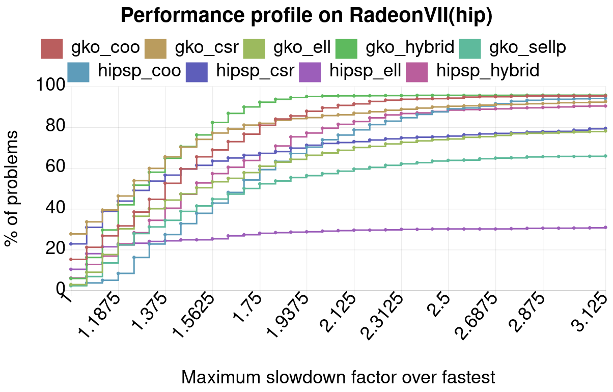
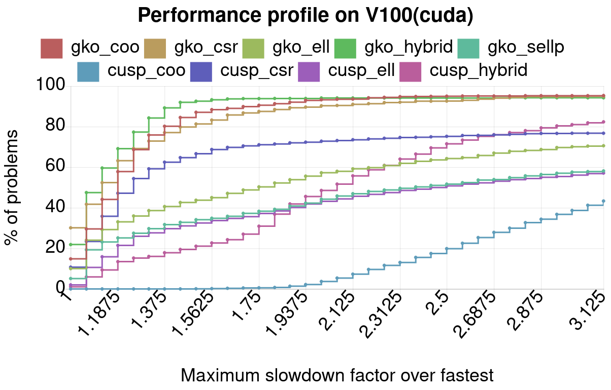
Figure 6. Performance profile comparing the runtime of Ginkgo’s SpMV kernels with the vendor libraries on the AMD RadeonVII (left) and the NVIDIA V100 (right). The plain names represent the Ginkgo kernels, the “hipsp_” and “cusp_” labels refer to the vendor implementations in AMD’s hipSPARSE and NVIDIA’s cuSPARSE libraries, respectively.

7.3. SpMV kernel performance

We next evaluate the performance of the SpMV kernel for all matrices available in the Suite Sparse Matrix Collection (Saad, 2003; sui, 2020) on the AMD RadeonVII and the NVIDIA V100 GPU (Tsai et al., pted). For this purpose, we compare the performance profile of the SpMV kernels available in the Ginkgo library with their counterparts available in the NVIDIA cuSPARSE and the AMD hipSPARSE libraries. The performance profile indicates for how many test matrices from the Suite Sparse Matrix Collection a specific format is the fastest (maximum slowdown factor 1.0), and how well a specific format generalized. I.e., for a given “acceptable slowdown factor,” which percentage of the problems from the Suite Sparse Matrix Collection can be covered. The performance profiles reveal that Ginkgo’s kernels are at least competitive, and in many cases superior to the vendor libraries.

Solver	Read access volume	Write access volume
BiCGSTAB	$(5\cdot n+2\cdot nnz)\cdot VT+2\cdot nnz\cdot IT+\lceil{}iter/2\rceil{}\cdot((16\cdot n+2\cdot nnz)\cdot VT+2\cdot nnz\cdot IT)+\lfloor{}iter/2\rfloor{}\cdot((13\cdot n+2\cdot nnz)\cdot VT+2\cdot nnz\cdot IT)$	$(10\cdot n+6)\cdot VT+\lceil{}iter/2\rceil{}\cdot((4\cdot n+2)\cdot VT)+\lfloor{}iter/2\rfloor{}\cdot((4\cdot n+3)\cdot VT)$
CG	$(4\cdot n+2\cdot nnz)\cdot VT+2\cdot nnz\cdot IT+iter\cdot((15\cdot n+2\cdot nnz)\cdot VT+2\cdot nnz\cdot IT)$	$(5\cdot n+2)\cdot VT+iter\cdot((5\cdot n+2)\cdot VT)$
CGS	$(5\cdot n+2\cdot nnz)\cdot VT+2\cdot nnz\cdot IT+\lceil{}iter/2\rceil{}\cdot((14\cdot n+2\cdot nnz)\cdot VT+2\cdot nnz\cdot IT)+\lfloor{}iter/2\rfloor{}\cdot((6\cdot n+2\cdot nnz)\cdot VT+2\cdot nnz\cdot IT)$	$(10\cdot n+2)\cdot VT+\lceil{}iter/2\rceil{}\cdot(6\cdot n+3)\cdot VT+\lfloor{}iter/2\rfloor{}\cdot(4\cdot n\cdot VT)$
FCG	$(4\cdot n+2\cdot nnz)\cdot VT+2\cdot nnz\cdot IT+iter\cdot((17\cdot n+2\cdot nnz)\cdot VT+2\cdot nnz\cdot IT)$	$(6\cdot n+3)\cdot VT+iter\cdot((6\cdot n+3)\cdot VT)$
GMRES	$(11\cdot n+2\cdot nnz+5/2\cdot r+n\cdot r+r^{2}/2+1)\cdot VT+2\cdot nnz\cdot IT+\lfloor{}iter/k\rfloor{}\cdot((1+5/2\cdot k+10\cdot n+2\cdot nnz+k^{2}/2+k\cdot n)\cdot VT+2\cdot nnz\cdot IT)+iter\cdot((7\cdot n+5+2\cdot nnz)\cdot VT+2\cdot nnz\cdot IT+8)+iter_{r}\cdot((4\cdot n+4)\cdot VT)$	$(6\cdot n+r+2\cdot k+3)\cdot VT+8+\lfloor{}iter/k\rfloor{}\cdot((k+6\cdot n+2)\cdot VT+8)+iter\cdot((4\cdot n+8)\cdot VT+8)+iter_{r}\cdot((n+2)\cdot VT)$

Table 2. Memory access volume of a full run of the distinct solver. Here $VT$ is the value type size in bytes (e.g., for double it is 8 bytes); $IT$ is value type for the index type; and $iter$ is the number of iterations the solver does. In GMRES, $k$ is the Krylov dimension (or restart iteration setting); $r=iter\%k$; and $iter_{r}=\lfloor{}iter/k\rfloor{}*(k-1)*k/2+(iter\%k-1)*iter\%k/2$.

7.4. Ginkgo solver performance

Prior to evaluating the performance of Ginkgo’s Krylov solvers, we point out that Krylov solvers operating with sparse linear systems are memory-bound algorithms. For this reason, we initially assess the bandwidth efficiency of the implementations of the different Krylov solvers. Concretely, we select the COO matrix format for the SpMV kernel, and run the Krylov solvers without any preconditioner. In Table 2 we list the target Krylov solvers along with their memory access volume (as a function of the iteration count). The formula for the GMRES algorithm is more involved as we implement a variant enhanced with restart.

For the experimental evaluation, we run 10,000 solver iterations on 10 different but representative test matrices from the Suite Sparse collection. For GMRES, we set the restart parameter to 100. In Figure 7, we visualize the memory bandwidth usage of the different Krylov solvers for both a V100 GPU executing CUDA code and an AMD RadeonVII GPU executing HIP code. In each graph we indicate the experimental peak bandwidth achieved by a reference stream triad bandwidth benchmark (Deakin et al., 2016). Both test machines reach a very similar STREAM triad bandwidth ($809.8$ GB/s on RadeonVII vs $812.6$ GB/s on V100), although the theoretical bandwidth of the RadeonVII is higher ($1024$ GB/s on RadeonVII vs $900$ GB/s on V100). The bandwidth performance analysis reveals that the algorithms are achieving bandwidth rates in the range of $500$ to $700$ GB/s on the RadeonVII machine and $600$ to $800$ GB/s on the V100 machine. This means that the Ginkgo solver performance reaches more than $70\%$ of the observed bandwidth on the RadeonVII machine (slightly less for GMRES), whereas it is more than $80\%$ on the V100 machine. To better understand this performance discrepancy, in Table 3 we provide detailed bandwidth results on both machines for key operations. The machines show different behaviors: for the copy operation the RadeonVII reaches $6\%$ better performance than the V100, whereas for the dot operation it reaches $25\%$ less performance than the V100, most likely due to the lack of independent thread scheduling. The relatively poor performance for global reductions on the AMD GPU may explain the performance difference of the Ginkgo solvers between the two machines, as global reductions are essential components of any Krylov solver.

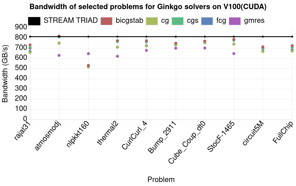
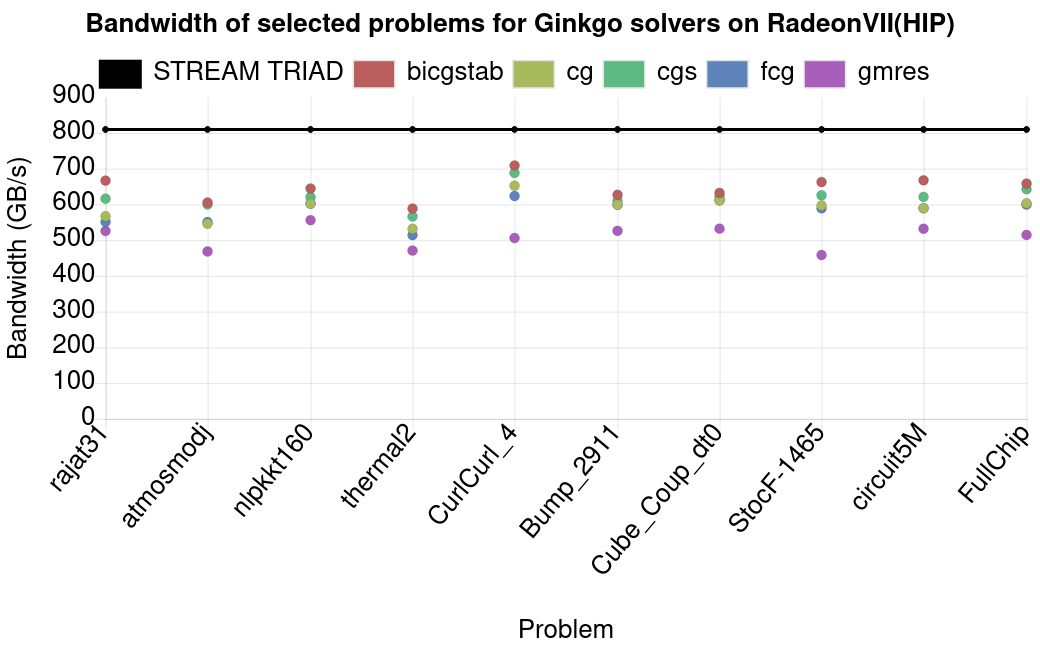
Figure 7. Memory efficiency of Ginkgo’s Krylov solvers.

Operation	V100 performance (GB/s)	RadeonVII performance (GB/s)
Copy	790.475	841.669
Mul	787.301	841.934
Add	811.312	806.632
Triad	812.617	809.754
Dot	844.321	635.677

Table 3. Stream bandwidth results from (Deakin et al., 2016) on the V100 and RadeonVII machines for key operations.

7.5. Ginkgo preconditioner performance

Ginkgo provides both (block-Jacobi type) preconditioners based on diagonal scaling and (ILU type) incomplete factorization preconditioners. Ginkgo’s ILU preconditioner technology is spearheading the community, including ParILUT, the first threshold-based ILU preconditioner for GPU architectures (Anzt et al., 2019d). This preconditioner approximates the values of the preconditioner via fixed-point iterations while dynamically adapting the sparsity pattern to the matrix properties (Anzt et al., 2018a). Depending on the matrix characteristics, this preconditioner can significantly accelerate the solution process of linear system solves; see Figure 8.

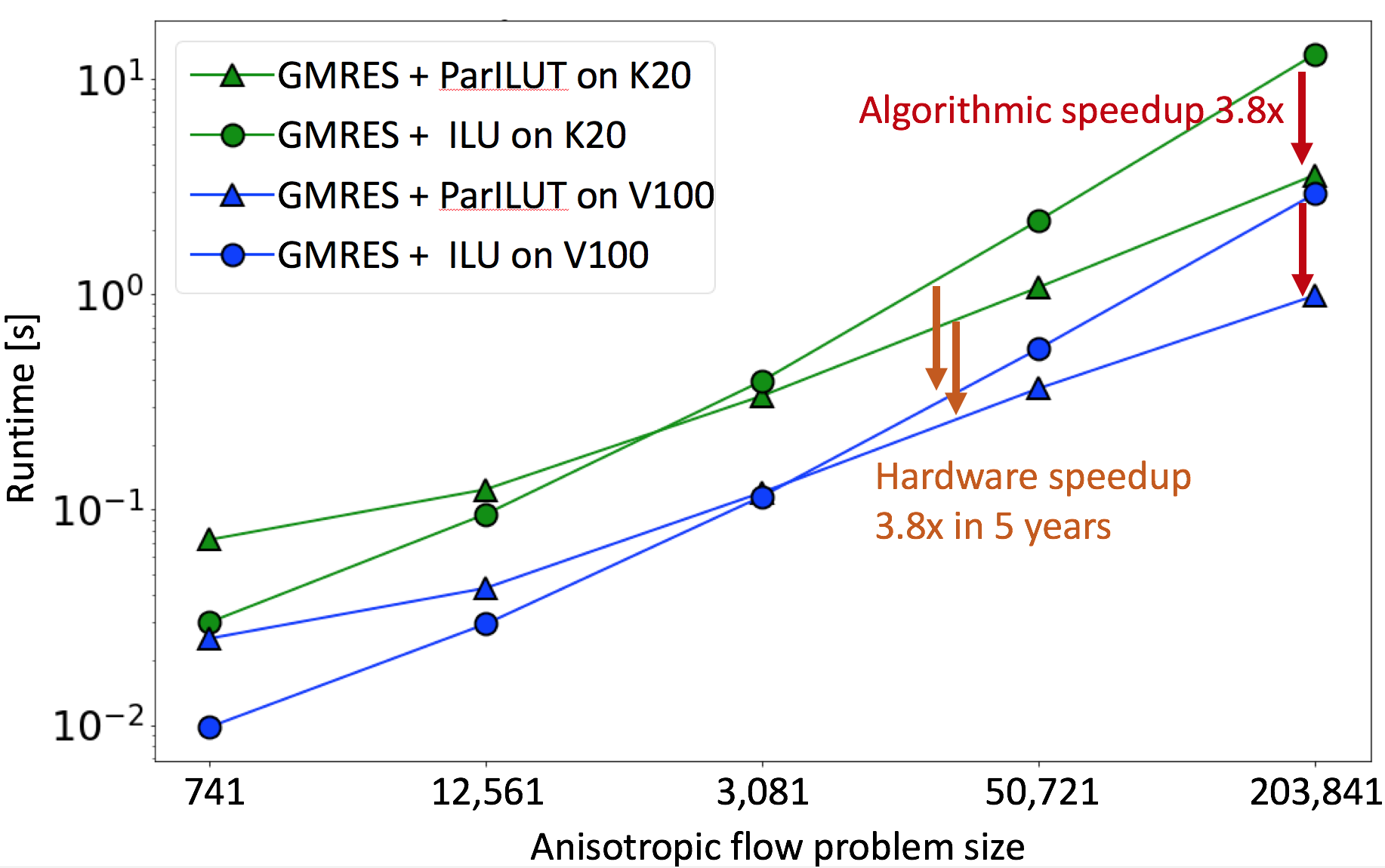
Figure 8. Time-to-solution comparison between standard ILU preconditioning (NVIDIA’s cuSPARSE) and Ginkgo’s ParILUT for solving anisotropic flow problems on two NVIDIA GPU generations. The GMRES solver is taken from the Ginkgo library.

Advanced techniques for the ILU preconditioner generation are complemented with fast triangular solvers, including iterative methods (Anzt et al., 2015; Goebel et al., pted) and the approximation of the inverse of the triangular factors via a sparse matrix (incomplete sparse approximate inverse preconditioning (Anzt et al., 2018b)).

Figure 9. Performance of the block-Jacobi preconditioner generation on the NVIDIA V100 GPU. The preconditioner generation includes the Gauss-Jordan elimination featuring pivoting, the condition number calculation and exponent range analysis, the storage format optimization, the format conversion, and the preconditioner storage in GPU main memory. The Different bars for each size represent the distinct memory precision scenarios and the scenarios where the performance data includes the automatic precision detection based on the block condition number and exponent range.

The block-Jacobi preconditioner available in Ginkgo outperforms its competitors by automatically adapting the memory precision to the numerical requirements, therewith reducing the memory access time of the memory-bound preconditioner application (Anzt et al., 2019c; Flegar et al., tted). The inversion of the diagonal block is realized via a heavily-tuned batched variable size Gauss-Jordan elimination (Anzt et al., 2019b); see Figure 9.

8. Conclusions and perspectives

Ginkgo is a modern C++-based sparse linear algebra library for GPU-centric HPC architectures with many appealing features including the Linear Operator abstraction, which fosters easy adoption of the library. Some other aspects that we have elaborated on include the execution control, memory management via smart pointers, software quality measures, and library extensibility. We have also provided example codes for software integration into the deal.ii and MFEM finite element ecosystems, and demonstrated the high performance of Ginkgo on high end GPU architectures. We believe that the design of the library and the sustainability measures that are taken as part of the development process have the potential to become role models for the future efforts on scientific software packages.

References

- (1)
- sui (2020) 2020. Suite Sparse Matrix Collection. http://faculty.cse.tamu.edu/davis/suitesparse.html.
- mix (2020) accessed in April 2020. Mix In. Portland Pattern Repository. https://wiki.c2.com/?MixIn
- obj (2020) accessed in April 2020. Object Slicing. Portland Pattern Repository. https://wiki.c2.com/?ObjectSlicing
- xsd (2020a) accessed in April 2020a. xSDK Examples https://xsdk.info/release-0-5-0/.
- xsd (2020b) accessed in April 2020b. xSDK: Extreme-scale Scientific Software Development Kit https://xsdk.info/.
- bss (2018) accessed in August 2018. Better Scientific Software (BSSw) https://bssw.io/.
- goo (2018) accessed in August 2018. Google Test https://github.com/google/googletest.
- Alzetta et al. (2018) G. Alzetta, D. Arndt, W. Bangerth, V. Boddu, B. Brands, D. Davydov, R. Gassmoeller, T. Heister, L. Heltai, K. Kormann, M. Kronbichler, M. Maier, J.-P. Pelteret, B. Turcksin, and D. Wells. 2018. The deal.II Library, Version 9.0. Journal of Numerical Mathematics 26, 4 (2018), 173–183. https://doi.org/10.1515/jnma-2018-0054
- Anderson et al. (1999) E. Anderson, Z. Bai, C. Bischof, S. Blackford, J. Demmel, J. Dongarra, J. Du Croz, A. Greenbaum, S. Hammarling, A. McKenney, and D. Sorensen. 1999. LAPACK Users’ Guide (third ed.). Society for Industrial and Applied Mathematics, Philadelphia, PA.
- Anderson et al. (2019) Robert Anderson, Julian Andrej, Andrew Barker, Jamie Bramwell, Jean-Sylvain Camier, Jakub Cerveny, Veselin Dobrev, Yohann Dudouit, Aaron Fisher, Tzanio Kolev, Will Pazner, Mark Stowell, Vladimir Tomov, Johann Dahm, David Medina, and Stefano Zampini. 2019. MFEM: a modular finite element methods library. arXiv e-prints, Article arXiv:1911.09220 (Nov. 2019), arXiv:1911.09220 pages. arXiv:cs.MS/1911.09220
- Anzt et al. (2019a) Hartwig Anzt, Yen-Chen Chen, Terry Cojean, Jack Dongarra, Goran Flegar, Pratik Nayak, Enrique S Quintana-Ortí, Yuhsiang M Tsai, and Weichung Wang. 2019a. Towards Continuous Benchmarking: An Automated Performance Evaluation Framework for High Performance Software. In Proceedings of the Platform for Advanced Scientific Computing Conference. 1–11.
- Anzt et al. (2015) Hartwig Anzt, Edmond Chow, and Jack Dongarra. 2015. Iterative sparse triangular solves for preconditioning. In European Conference on Parallel Processing. Springer, Berlin, Heidelberg, 650–661.
- Anzt et al. (2018a) Hartwig Anzt, Edmond Chow, and Jack Dongarra. 2018a. ParILUT—A New Parallel Threshold ILU Factorization. SIAM Journal on Scientific Computing 40, 4 (2018), C503–C519.
- Anzt et al. (2019c) Hartwig Anzt, Jack Dongarra, Goran Flegar, Nicholas J Higham, and Enrique S Quintana-Ortí. 2019c. Adaptive precision in block-Jacobi preconditioning for iterative sparse linear system solvers. Concurrency and Computation: Practice and Experience 31, 6 (2019), e4460.
- Anzt et al. (2019b) Hartwig Anzt, Jack Dongarra, Goran Flegar, and Enrique S Quintana-Ortí. 2019b. Variable-size batched Gauss–Jordan elimination for block-Jacobi preconditioning on graphics processors. Parallel Comput. 81 (2019), 131–146.
- Anzt et al. (2018b) Hartwig Anzt, Thomas K Huckle, Jürgen Bräckle, and Jack Dongarra. 2018b. Incomplete sparse approximate inverses for parallel preconditioning. Parallel Comput. 71 (2018), 1–22.
- Anzt et al. (2019d) Hartwig Anzt, Tobias Ribizel, Goran Flegar, Edmond Chow, and Jack Dongarra. 2019d. ParILUT—A Parallel Threshold ILU for GPUs. In 2019 IEEE International Parallel and Distributed Processing Symposium (IPDPS). IEEE, 231–241.
- Chow et al. (2015) Edmond Chow, Hartwig Anzt, and Jack Dongarra. 2015. Asynchronous iterative algorithm for computing incomplete factorizations on GPUs. In International Conference on High Performance Computing. Springer, Cham, 1–16.
- Coplien (1995) James O. Coplien. 1995. Curiously Recurring Template Patterns. C++ Report (1995).
- Deakin et al. (2016) Tom Deakin, James Price, Matt Martineau, and Simon McIntosh-Smith. 2016. GPU-STREAM v2.0: Benchmarking the Achievable Memory Bandwidth of Many-Core Processors Across Diverse Parallel Programming Models. In High Performance Computing, Michela Taufer, Bernd Mohr, and Julian M. Kunkel (Eds.). Springer International Publishing, Cham, 489–507.
- Flegar et al. (tted) Goran Flegar, Hartwig Anzt, Terry Cojean, and Enrique S. Quintana-Ortí. submitted. Customized-Precision Block-Jacobi Preconditioning for Krylov Iterative Solvers on Data-Parallel Manycore Processors. ACM TOMS (submitted).
- Gamma et al. (1994) Erich Gamma, Richard Helm, Ralph Johnson, and John M. Vlissides. 1994. Design Patterns: Elements of Reusable Object-Oriented Software (1 ed.). Addison-Wesley Professional. http://www.amazon.com/Design-Patterns-Elements-Reusable-Object-Oriented/dp/0201633612/ref=ntt_at_ep_dpi_1
- Goebel et al. (pted) Fritz Goebel, Hartwig Anzt, Terry Cojean, Goran Flegar, and Enrique S. Quintana-Ortí. accepted. Multiprecision block-Jacobi for Iterative Triangular Solves. EuroPar Conference 2020 (accepted).
- Jagode et al. (2019) Heike Jagode, Anthony Danalis, Hartwig Anzt, and Jack Dongarra. 2019. PAPI software-defined events for in-depth performance analysis. The International Journal of High Performance Computing Applications 33, 6 (2019), 1113–1127.
- Johnson et al. (1995) R. Johnson, E. Gamma, J. Vlissides, and R. Helm. 1995. Design Patterns: Elements of Reusable Object-Oriented Software. Addison-Wesley. https://books.google.de/books?id=iyIvGGp2550C
- Lawson et al. (1979) C. L. Lawson, R. J. Hanson, D. R. Kincaid, and F. T. Krogh. 1979. Basic Linear Algebra Subprograms for Fortran Usage. ACM Trans. Math. Softw. 5, 3 (Sept. 1979), 308–323. https://doi.org/10.1145/355841.355847
- Saad (2003) Y. Saad. 2003. Iterative Methods for Sparse Linear Systems (second ed.). Society for Industrial and Applied Mathematics. https://doi.org/10.1137/1.9780898718003
- Tsai et al. (pted) Yuhsiang M. Tsai, Terry Cojean, and Hartwig Anzt. accepted. Sparse Linear Algebra on AMD and NVIDIA GPUs – The Race is on. ISC High Performance 2020 (accepted).